Fast Dual Variational Inference for Non-Conjugate
Latent Gaussian Models

Abstract

Latent Gaussian models (LGMs) are widely used in statistics and machine learning. Bayesian inference in non-conjugate LGMs is difficult due to intractable integrals involving the Gaussian prior and non-conjugate likelihoods. Algorithms based on variational Gaussian (VG) approximations are widely employed since they strike a favorable balance between accuracy, generality, speed, and ease of use. However, the structure of the optimization problems associated with these approximations remains poorly understood, and standard solvers take too long to converge. We derive a novel dual variational inference approach that exploits the convexity property of the VG approximations. We obtain an algorithm that solves a convex optimization problem, reduces the number of variational parameters, and converges much faster than previous methods. Using real-world data, we demonstrate these advantages on a variety of LGMs, including Gaussian process classification, and latent Gaussian Markov random fields.

1 Introduction

Latent Gaussian models (LGM) are ubiquitous in machine learning and statistics (e.g., Gaussian process models, Bayesian generalized linear models, dynamical systems with non-Gaussian observations, robust PCA, and non-conjugate matrix factorization). In many real-world applications, the likelihood is not conjugate to the Gaussian distribution, making exact Bayesian inference intractable. These modern applications, especially those with large latent dimensionality and number of observations, require fast, robust, and reliable algorithms for approximate inference.

In this context, algorithms based on variational Gaussian (VG) approximations are growing in popularity (opper2009variational; challis2011concave; Lazaro:11; Honkela:11), since they strike a favorable balance between accuracy, generality, speed, and ease of use. However, compared to other approximations such as that of Seeger:11, the structure of optimization problems associated with VG approximations remains poorly understood, and standard solvers for optimization take too long to converge.

While some variants of VG inference are convex (Khan12nips), they require $O(L^{2})$ variational parameters to be optimized, where $L$ is the dimensionality of the latent Gaussian vector. This slows down the optimization dramatically. One approach is to restrict the covariance representations up front, whether by naive mean field (braun2010variational; knowles2011non) or restricted Cholesky assumptions (challis2011concave). Unfortunately, this can result in considerable loss in accuracy, since typical LGMs, such as Gaussian processes, are tightly coupled. Another approach is to reduce the number of parameters to $O(N)$, where $N$ is the dimension of the observation vector, using an exact covariance parameterization (opper2009variational). This reparameterization destroys the convexity of the original problem, and very slow convergence is typically observed (Khan12nips). A recent coordinate-ascent method improves upon the state of the art (Khan12nips), but is restricted to Gaussian process models only and uses inefficient low-rank matrix updates.

We propose a dual decomposition approach that allows us to reduce the number of parameters to $O(N)$ while retaining convexity. The new dual optimization problem can be solved very rapidly with standard methods for smooth optimization. Using real-world data, we demonstrate that our algorithm converges much faster than the state of the art on a variety of LGMs. Unlike the approach of Khan12nips, our algorithm is generic and is not restricted to Gaussian processes.

2 Latent Gaussian Models

Given a vector of observations $\boldsymbol{y}\in{\cal Y}^{N}$, the dependencies among its components can be modeled using a latent vector $\boldsymbol{z}\in\mathbb{R}^{L}$. Here, the set $\cal Y$ is the domain of each observation, e.g., for binary observations, ${\cal Y}=\{0,1\}$. The latent vector $\boldsymbol{z}$ is assumed to follow a Gaussian distribution $p(\boldsymbol{z})=\mbox{${\cal N}$}(\boldsymbol{z}|\boldsymbol{\mu},\boldsymbol{\Sigma})$. The likelihood has the general form

$$p(\boldsymbol{y}|\boldsymbol{z}) =\prod_{n=1}^{N}p(y_{n}|\eta_{n}),\quad\boldsymbol{\eta}=\boldsymbol{W}\boldsymbol{z},$$ (1)

where $\boldsymbol{W}\in\mathbb{R}^{N\times L}$. Model parameters $\boldsymbol{\theta}$ consist of parameters required to specify $\boldsymbol{\mu}$, $\boldsymbol{\Sigma}$, $\boldsymbol{W}$, as well as parameters of the distribution $p(y_{n}|\eta_{n})$. All densities are implicitly conditioned on $\boldsymbol{\theta}$, which we suppress from the notation. Also note that $\eta_{n}$ can be a vector but we restrict ourselves to scalar $\eta_{n}$. Our results can be easily extended to the vector case.

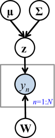
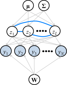
Figure 1: The graphical model for latent Gaussian models shown in left figure, and expanded in the right figure to explicitly show the correlation in the latent vector $\boldsymbol{z}$ induced due to a non-diagonal $\boldsymbol{\Sigma}$.

Many models used in statistics and machine learning are instances of LGMs. Several examples are listed in Table 1, and an extensive list can be found in emtThesis. Bayesian generalized linear models constitute one such example, where we assume a latent Gaussian weight vector and use exponential family likelihoods with natural parameter $\eta_{n}$. Similarly, latent Gaussian Markov random fields (GMRF) model spatial correlations by using a GMRF with a sparse inverse covariance matrix $\boldsymbol{\Sigma}^{-1}$, along with an exponential family likelihood to model non-normal observations (Rue05). For example, count data with spatial dependence (e.g., incidences of a disease in different regions of a country) can be modeled using a Poisson likelihood with rate $r_{n}=\exp(\eta_{n})$. The log-Gaussian Cox process is a non-parameteric generalization of this setting (Rue09). Other non-parameteric examples are Gaussian process (GP) models, where observation pairs $\{y_{n},\boldsymbol{x}_{n}\}$ are modelled via a latent Gaussian process $z(\boldsymbol{x})$ with the prior specified by mean and covariance functions.

In Bayesian inference, we wish to compute expectations with respect to the posterior distribution

$$p(\boldsymbol{z}|\boldsymbol{y}) \propto\prod\nolimits_{n=1}^{N}p(y_{n}|\eta_{n})\mbox{${\cal N}$}(\boldsymbol{z}|\boldsymbol{\mu},\boldsymbol{\Sigma}).$$ (2)

For example, prediction of a new observation $y_{*}$ can be obtained by computing the expectation $p(y_{*}|\boldsymbol{y})=\int p(y_{*}|\boldsymbol{\eta})p(\boldsymbol{z}|\boldsymbol{y})\,d\boldsymbol{z}$. Another important task is computation of the marginal likelihood

$$p(\boldsymbol{y}) =\int\prod\nolimits_{n=1}^{N}p(y_{n}|\eta_{n})\mbox{${\cal N}$}(\boldsymbol{z}|\boldsymbol{\mu},\boldsymbol{\Sigma})\,d\boldsymbol{z}.$$ (3)

For example, parameters $\boldsymbol{\theta}$ can be learned by maximizing the log of the marginal likelihood, $\log p(\boldsymbol{y})$. This is also referred to as empirical Bayes or automatic relevance determination (ARD) (Tipping:01; Rasmussen06).

For non-Gaussian likelihoods, both of these tasks are intractable. Applications in practice demand good approximations that scale favorably in $N$ and $L$.

Model	Data	$\boldsymbol{z}$	$\boldsymbol{\theta}$	$N$	$L$	Remarks
Bayesian Logistic	$\{y_{n},\boldsymbol{x}_{n}\}$	Regression weights	${\boldsymbol{\mu},\boldsymbol{\Sigma}}$	#Obs	#Features	Row of $\boldsymbol{W}$
Regression		$y_{n}\leftarrow f(\boldsymbol{z}^{T}\boldsymbol{x}_{n})$				$\boldsymbol{w}_{n}=\boldsymbol{x}_{n}$
Gaussian Process	$\{y_{n},\boldsymbol{x}_{n}\}$	Regression function	${s,\sigma}$	#Obs	#Features	$\boldsymbol{W}=\boldsymbol{I}$
Classification		$y_{n}\leftarrow f(z_{n})$				$N=L$
Gaussian Markov	$\{y_{n}\}$	Latent Gaussian field	${k_{v},k_{u}}$	#Obs	# Latent
Random Field		$y_{n}\leftarrow f(\boldsymbol{z}_{n})$			dims
Probabilistic PCA	$\{y_{ni}\}$	Latent factors	$\boldsymbol{W}$	#Obs	#Latent	$N>L$
		$y_{n}\leftarrow f(\boldsymbol{w}_{i}^{T}\boldsymbol{z}_{n})$		dims	factors	$\boldsymbol{\mu}=\boldsymbol{0},\boldsymbol{\Sigma}=\boldsymbol{I}$

Table 1: Examples of LGM. Each column is a quantity from our generic LGM definition. Each row shows corresponding quantities for a model. First two models are supervised and the last two are unsupervised. For columns 2 and 3, $n$ ranges over $1$ to $N$ and $\{a_{n}\}$ denotes the set of variables indexed by all values of $n$. $y\leftarrow f(z)$ implies that $y$ can be generated using some function $f$ of $z$. In last three columns, ‘Obs’ means observations, ‘Dims’ means dimensions, and ‘#’ represents the number of a quantity. For GP, $s$ and $\sigma$ are hyperparameters of the covariance function. Similarly, $k_{u}$ and $k_{v}$ are hyperparameters for the latent field. See Section LABEL:sec:exper for details. For PPCA, the subscript $i$ indexes the observation vector.

3 Variational Gaussian Inference

In the variational Gaussian approximation (opper2009variational), we assume the posterior to be a Gaussian $q(\boldsymbol{z})=\mbox{${\cal N}$}(\boldsymbol{z}|\boldsymbol{m},\boldsymbol{V})$. The posterior mean $\boldsymbol{m}$ and covariance $\boldsymbol{V}$ form the set of variational parameters, and are chosen to maximize the variational lower bound to the log marginal likelihood shown in Eq. 5. To get this lower bound, we first multiply and divide by $q(\boldsymbol{z})$ in Eq. 4, and then use Jensen’s inequality and the concavity of $\log$ (we denote the expectation with respect to $q(\boldsymbol{z})$ by $\mathrm{E}_{q(z)}$):

$$\log p(\boldsymbol{y}) =\log\int q(\boldsymbol{z})\frac{\prod_{n}p(y_{n}|\eta_{n})p(\boldsymbol{z})}{q(\boldsymbol{z})}\,d\boldsymbol{z}$$ (4)

$$\geq\mathrm{E}_{q(z)}\left[\log\frac{\prod_{n}p(y_{n}|\eta_{n})p(\boldsymbol{z})}{q(\boldsymbol{z})}\right].$$ (5)

The lower bound can be simplified further, and variational parameters $\boldsymbol{m}$ and $\boldsymbol{V}$ can be obtained by maximizing it:

$$\max_{\boldsymbol{m},\boldsymbol{V}\succ\boldsymbol{0}}-\mathrm{D}[q(\boldsymbol{z})\,\|\,p(\boldsymbol{z})]-\sum_{n=1}^{N}\mathrm{E}_{q(\eta_{n})}[-\log p(y_{n}|\eta_{n})],$$ (6)

where

$$\mathrm{D}[q\,\|\,p] =\mathrm{E}_{q}[\log q(\boldsymbol{z})-\log p(\boldsymbol{z})]$$ (7)

$$q(\eta_{n}) =\mbox{${\cal N}$}(\bar{m}_{n},\bar{v}_{n})$$ (8)

$$\bar{\boldsymbol{m}} =\boldsymbol{W}\boldsymbol{m},\quad\bar{\boldsymbol{v}}=\operatorname{diag}(\boldsymbol{W}\boldsymbol{V}\boldsymbol{W}^{T}).$$ (9)

See Eqs. 4–7 in Khan12aistats for details of this derivation.

The first term in Eq. 6 is the relative entropy, and is jointly concave in $(\boldsymbol{m},\boldsymbol{V})$. The second term $\mathrm{E}_{q(\eta_{n})}[-\log p(y_{n}|\eta_{n})]$ is not always available in closed form. We assume in this paper that, in such cases, we can evaluate an upper bound $f_{n}$ to this term, i.e.,

$$\mathrm{E}_{q(\eta_{n})}[-\log p(y_{n}|\eta_{n})]\leq f_{n}(\bar{m}_{n},\bar{v}_{n}).$$ (10)

This is also known as the local variational bound (LVB). We assume that $f_{n}$ is differentiable and—most importantly—convex. We discuss a few such LVBs in Section LABEL:sec:details; see emtThesis for an extensive list.

The resulting optimization problem is shown below in Eq. 11 and is expanded in Eq. 3:

$$\max_{\boldsymbol{m},\boldsymbol{V}\succ\boldsymbol{0}}-\mathrm{D}[q(\boldsymbol{z})\,\|\,p(\boldsymbol{z})]-\sum_{n=1}^{N}f_{n}(\bar{m}_{n},\bar{v}_{n})$$ (11)

$$:=\mbox{$\frac{1}{2}$}[\log|\boldsymbol{V}|-\operatorname{tr}(\boldsymbol{V}\boldsymbol{\Sigma}^{-1})-(\boldsymbol{m}-\boldsymbol{\mu})^{T}\boldsymbol{\Sigma}^{-1}(\boldsymbol{m}-\boldsymbol{\mu})]$$

$$\qquad\qquad\qquad\qquad-\sum_{n=1}^{N}f_{n}(\bar{m}_{n},\bar{v}_{n})+\textrm{cnst}.$$ (12)

The above lower bound is strictly concave (braun2010variational; challis2011concave; emtThesis).

3.1 Related Work

A straight-forward approach is to solve Eq. 11 directly in $(\boldsymbol{m},\boldsymbol{V})$ (braun2010variational; challis2011concave; marlin2011piecewise; Khan12aistats). In practice, direct methods are slow and memory-intensive because of the very large number $L+L(L+1)/2$ of primal variables. challis2011concave show that for log-concave likelihoods $p(y_{n}|\eta_{n})$, the original problem Eq. 6 is jointly concave in $\boldsymbol{m}$ and the Cholesky factor of $\boldsymbol{V}$, and additional LVBs are not required. This fact, however, does not result in any reduction in number of parameters, and they propose to use factorizations of a restricted form, which negatively affects the approximation accuracy.

opper2009variational and nickisch2008approximations note that the optimal $\boldsymbol{V}_{*}$ must be of the form

$$\boldsymbol{V}_{*}=(\boldsymbol{\Sigma}^{-1}+\boldsymbol{W}^{T}(\operatorname{diag}\boldsymbol{\lambda})\boldsymbol{W})^{-1},$$ (13)

which suggests reparameterizing Eq. 11 in terms of $L+N$ parameters $(\boldsymbol{m},\boldsymbol{\lambda})$, where $\boldsymbol{\lambda}$ is the new variable. However, the problem is non-concave in this alternative parameterization (Khan12nips). Moreover, as shown in (Khan12nips) and our experiments here, convergence can be exceedingly slow. The coordinate-ascent algorithm proposed in (Khan12nips) solves the problem of convergence, but seems limited to the case $N=L$ and $\boldsymbol{W}=\boldsymbol{I}$. In addition, it requires $N$ rank-one updates of $\boldsymbol{V}$ per iteration, which is slow on modern architectures optimized for block-matrix computations.

A range of different deterministic inference approximations apply to latent Gaussian models. The local variational method is convex for log-concave potentials and can be solved at very large scales (Seeger:11). However, it applies to super-Gaussian potentials only. The bound it maximizes is provably less tight than Eq. 6 (Seeger:09c; challis2011concave), and it leads to worse results than the variational Gaussian approximation in general (nickisch2008approximations; emtThesis). A key interpretation of this method is that it can be seen as one way to generate LVBs (for super-Gaussian potentials), which can be used in our VG setup (Seeger:09c). Expectation propagation (Minka:01a; Seeger:07d) is more general and can be more accurate than most other approximations mentioned here. Based on a saddlepoint rather than an optimization problem, the standard EP algorithm does not always converge and can be numerically unstable. Among these alternatives, the variational Gaussian approximation stands out as a compromise between accuracy and good algorithmic properties, which is widely used beyond latent Gaussian model applications as well (Lazaro:11; Honkela:11).

4 Dual Variational Inference

In this section, we show how Eq. 11 can be solved using a convex dual formulation in only $N$ variational parameters. As shown in our experiments, the novel formulation admits simple algorithms which converge much more rapidly and have a lower per-iteration cost than previous methods reviewed above. We achieve this by dual decomposition: decoupling the two terms in Eq. 11 by equality constraints, and then forming the Lagrangian dual. To be precise, we first introduce two new variables $h_{n},\rho_{n}\in\mathbb{R}$ for each $n$ and introduce constraints $h_{n}=\bar{m}_{n}$ and $\rho_{n}=\bar{v}_{n}$. The resulting (equivalent) optimization problem can be written as

$$\max_{\boldsymbol{m},\boldsymbol{V},\boldsymbol{h},\boldsymbol{\rho}}-\mathrm{D}[q(\boldsymbol{z})\,\|\,p(\boldsymbol{z})]-\sum\nolimits_{n=1}^{N}f_{n}(h_{n},\rho_{n})$$ (14)

$$\qquad\qquad\text{s.t.}\;\;\boldsymbol{h}=\boldsymbol{W}\boldsymbol{m},\quad\boldsymbol{\rho}=\operatorname{diag}(\boldsymbol{W}\boldsymbol{V}\boldsymbol{W}^{T}).$$

Next, we introduce dual variables $\boldsymbol{\alpha},\boldsymbol{\lambda}\in\mathbb{R}^{N}$ associated to these constraints, and form the corresponding Lagrangian

$${\cal L}=-\mathrm{D}[q(\boldsymbol{z})\,\|\,p(\boldsymbol{z})]-\sum\nolimits_{n=1}^{N}f_{n}(h_{n},\rho_{n})$$ (15)

$$\qquad+\boldsymbol{\alpha}^{T}(\boldsymbol{h}-\boldsymbol{W}\boldsymbol{m})+{\textstyle\frac{1}{2}}\boldsymbol{\lambda}^{T}(\boldsymbol{\rho}-\operatorname{diag}(\boldsymbol{W}\boldsymbol{V}\boldsymbol{W}^{T})).$$

Strong duality holds because the constraints are affine, and so the solution to the original problem can be found by minimizing the Lagrangian dual with respect to $(\boldsymbol{\alpha},\boldsymbol{\lambda})$, i.e.,

$$\min_{\boldsymbol{\alpha},\boldsymbol{\lambda}}\ \mathcal{D}(\boldsymbol{\alpha},\boldsymbol{\lambda})=\min_{\boldsymbol{\alpha},\boldsymbol{\lambda}}\max_{\boldsymbol{m},\boldsymbol{V},\boldsymbol{h},\boldsymbol{\rho}}{\cal L}.$$ (16)

The advantage of this formulation is that we can solve analytically for $(\boldsymbol{m},\boldsymbol{V})$ and $(\boldsymbol{h},\boldsymbol{\rho})$, and the resulting dual $\mathcal{D}(\boldsymbol{\alpha},\boldsymbol{\lambda})$ is available in closed form. Since $\boldsymbol{\alpha}$ and $\boldsymbol{\lambda}$ are length $N$ vector, the dual minimization involves only $O(N)$ parameters.

Derivations of the following statements are given in the Appendix. The unique maximizer with respect to $(\boldsymbol{m},\boldsymbol{V})$ is given by

$$\boldsymbol{m}_{*} =\boldsymbol{\mu}-\boldsymbol{\Sigma}\boldsymbol{W}^{T}\boldsymbol{\alpha}$$ (17)

$$\boldsymbol{V}_{*} =\boldsymbol{A}_{\boldsymbol{\lambda}}^{-1}:=(\boldsymbol{\Sigma}^{-1}+\boldsymbol{W}^{T}(\operatorname{diag}\boldsymbol{\lambda})\boldsymbol{W})^{-1}.$$ (18)

Importantly, $\boldsymbol{V}_{*}$ has precisely the economical form pointed out by opper2009variational.

Maximization over $(\boldsymbol{h},\boldsymbol{\rho})$ is also available in closed form. Collecting the terms involving $(h_{n},\rho_{n})$ in Eq. 15, we get the following optimization problem,

$$f_{n}^{*}(\alpha_{n},\lambda_{n}):=\max_{h_{n},\rho_{n}}\alpha_{n}h_{n}+\lambda_{n}\rho_{n}/2-f_{n}(h_{n},\rho_{n}),$$ (19)

which is in fact the $f_{n}^{*}$ the Fenchel conjugate of $f_{n}$ (Rockafellar:70), and is convex and well-defined due to the convexity of $f_{n}$. For many likelihoods (and LVBs), $f_{n}^{*}$ is available in closed form. We give several examples in Section LABEL:sec:details, summarized in Table LABEL:tab:fenchelDual.

Note that the effective domain of $f_{n}^{*}$ (i.e., values of $(\alpha,\lambda)$ for which $f_{n}^{*}$ is finite) may be restricted. We give details of this and show the effective domain of $f_{n}^{*}(\alpha_{n},\lambda_{n})$ for several commonly used likelihoods in Section LABEL:sec:details. We denote the effective domain of $f_{n}^{*}$ by $\mathcal{S}$.

Plugging in Eq. 17, 18, and 19 into Eq. 15 and ignoring the constants, directly gives us the optimization problem

$$\min_{\boldsymbol{\alpha},\boldsymbol{\lambda}\in\mathcal{S}}\mbox{$\frac{1}{2}$}\boldsymbol{\alpha}^{T}\widetilde{\boldsymbol{\Sigma}}\boldsymbol{\alpha}-\widetilde{\boldsymbol{\mu}}^{T}\boldsymbol{\alpha}-\mbox{$\frac{1}{2}$}\log|\boldsymbol{A}_{\boldsymbol{\lambda}}|+\sum_{n=1}^{N}f_{n}^{*}(\alpha_{n},\lambda_{n}),$$ (20)

where $\widetilde{\boldsymbol{\mu}}=\boldsymbol{W}\boldsymbol{\mu}$ and $\widetilde{\boldsymbol{\Sigma}}=\boldsymbol{W}\boldsymbol{\Sigma}\boldsymbol{W}^{T}$.

This is a strictly convex optimization problem involving $2N$ parameters, in contrast to Eq. 11, which involves $O(L^{2})$ number of parameters. Given $(\boldsymbol{\alpha}_{*},\boldsymbol{\lambda}_{*})$ that minimizes the dual, the primal solution $(\boldsymbol{m}_{*},\boldsymbol{V}_{*})$ is obtained using Eq. 17 and 18. It might appear that minimizing the dual might be a difficult problem due to the constraints, but as we show later $f_{n}^{*}$, act as barrier functions, which simplify the optimization.