Deviation test construction and power comparison for marked spatial point patterns

Abstract

The deviation test belong to core tools in point process statistics, where hypotheses are typically tested considering differences between an empirical summary function and its expectation under the null hypothesis, which depend on a distance variable $r$. This test is a classical device to overcome the multiple comparison problem which appears since the functional differences have to be considered for a range of distances $r$ simultaneously. The test has three basic ingredients: (i) choice of a suitable summary function, (ii) transformation of the summary function or scaling of the differences, and (iii) calculation of a global deviation measure. We consider in detail the construction of such tests both for stationary and finite point processes and show by two toy examples and a simulation study for the case of the random labelling hypothesis that the points (i) and (ii) have great influence on the power of the tests.

Key words: deviation test; marked point process; marking model; mark-weighted $K$-function; Monte Carlo test; multiple comparison; random labelling; simulation study

1.  Introduction

Testing statistical hypotheses is an important step in building statistical models. Often it is checked whether the data deviate significantly from a null model. In point process statistics, typical null models are complete spatial randomness (CSR), independent marking or some fitted model. Unlike in classical statistics, where null models are typically represented by a single hypothesis, the hypotheses in spatial statistics have a spatial dimension and therefore a multiple character. Usually a summary function $S(r)$ is employed in the test, where $r$ is a distance variable. A typical example is Ripley’s $K$-function.

The tests are based on the differences of empirical and theoretical values of $S(r)$, which are called “residuals” in the following. A problem is how to handle the residuals for different values of $r$. One possibility is construction of envelopes around the theoretical summary function and to look if the empirical summary function is completely between the envelopes. This very popular method, which goes back to Ripley (1977), has a difficult point: to guarantee a given significance level and to determine $p$-values, see the discussion in Loosmore and Ford (2006) and Grabarnik et al. (2011). An alternative approach was proposed by Diggle (1979), who introduced statistics which compress information from the residuals for intervals of $r$-values to a scalar. This approach has analogues in classical statistics, namely the Kolmogorov-Smirnov and von Mises tests. In the present paper tests in Diggle’s spirit are called deviation tests.

Though Diggle’s procedure is accepted as a standard in spatial point process statistics, to our knowledge there are no studies which explore its properties systematically. Several power comparisons for different forms of deviation tests have been reported (e.g. Ripley 1979; Gignoux et al. 1999; Thönnes and van Lieshout 1999; Baddeley et al. 2000; Grabarnik and Chiu 2002; Ho and Chiu 2006, 2009), but these investigations concern only specific issues. In the present paper, we consider the construction of deviation tests in more detail and systematically and give general recommendations for their use, for stationary as well as for finite point processes.

Recall that a classical deviation test in point process statistics is based on a summary function $S(r)$ for the null model and its unbiased estimator $\hat{S}(r)$. If there would be a priori a value of distance $r$ which is of main interest, then one could proceed as in classical tests by comparing the empirical value $\hat{S}(r)$ with $S(r)$ for this $r$, i.e. to consider the residual $\hat{S}(r)-S(r)$. However, since usually such a single special distance $r$ is not given, one would like to consider the residuals simultaneously for all distances $r$ in some interval $I=[r_{\text{min}},r_{\text{max}}]$. Thus, one is confronted with a situation typical for multiple hypothesis testing (or multiple comparisons), see Bretz et al. (2010). A deviation test resolves the multiple hypothesis testing problem by summarizing the residuals for all $r$ in $I$ into a single number by some deviation measure, e.g. the maximum absolute residual in $I$.

A summary function frequently used in point process statistics for stationary processes and in deviation tests is Ripley’s $K$-function (Ripley 1976, 1977). Since Besag (1977) found that, under CSR, the $L$-function resulting from the transformation $\hat{K}(r)\rightarrow\sqrt{\hat{K}(r)/\pi}$ has a variance which is approximately constant over the distances $r$, the $L$-function became popular. Consequently, it is empirically well-accepted that a deviation test based on the $L$-function is “better” than a test based on the $K$-function. Variance-stabilising transformations are available also in other cases, see e.g. Schladitz and Baddeley (2000) and Grabarnik and Chiu (2002), whereas many summary functions such as the nearest neighbour distribution function ($D$- or $G$-function) and $J$-function (van Lieshout and Baddeley 1996) are employed without transformations.

We show that it is useful to use transformations and additional scalings of the residuals, particularly relative to their variances, in order to uniform the contributions of residuals for different distances $r$.

Besides transformations and scaling also other elements of deviation tests have influence on its power. These are the basic choice of the summary function $S(r)$, the interval of distances $I$ and the deviation measure. We explore the role of these elements through a simulation study for an important test problem for marked point processes: checking the random labelling hypothesis, which says that the marks of a marked point pattern are independent. Note that this particular case contains all elements of a deviation test in point process statistics, for the stationary as well as for the finite case.

The rest of the paper is organized as follows. Section 2 explains the fundamentals of deviation tests in point process statistics, in a generalised form applicable also for non-stationary and finite processes and biased estimators. Section 3 then discusses the construction of deviation tests in detail, from the point of view of multiple testing. Section 4 describes the design for the simulation study, the results of which are reported in Section 5. Section 6 discusses the results and ends with recommendations for practical work.

2.  Preliminaries on point process statistics

The symbols $N=\{x_{i}\}$ and $N_{m}=\{[x_{i};m(x_{i})]\}$ denote a point process and a marked point process, respectively. The $x_{i}$ are the points, while $m(x_{i})$ is the mark of point $x_{i}$. In the present paper planar point processes are considered, but the main ideas hold true also for point processes in $\mathbb{R}^{d}$ for $d\geq 2$.

If $N$ and $N_{m}$ are stationary, they have an intensity which is denoted by $\lambda$. The mark distribution function is denoted by $F_{M}(m)$. Its mean and variance are $\mu_{m}$ and $\sigma^{2}_{m}$.

The statistical analysis is based on observations in a window $W$, which is a compact convex subset of $\mathbb{R}^{d}$. In the planar case the window is often a rectangle.

When distributional hypotheses for point processes have to be tested, deviation tests as suggested by Diggle (1979) are a popular tool. We consider these tests here in a generalised form. Such a test is based on a test function $T(r)$ that characterises in some way the spatial arrangement of the points and/or marks in the window $W$. There are many possibilities for such functions. In the classical case, a common choice for $T(r)$ is an unbiased estimator $\hat{S}(r)$ of some summary function $S(r)$, see e.g. Cressie (1993), Diggle (2003) and Illian et al. (2008) for examples. Popular functions for stationary processes in the case without marks are Ripley’s $K$-function, the nearest neighbour distance distribution function ($G$-function) and the empty space function/spherical contact distribution ($F$-function). For stationary marked point processes, various mark correlation functions including the mark-weighted $K$-functions are available. For non-stationary or finite processes analogues of stationary-case characteristics can be used.

Since deviation tests are in essence Monte Carlo tests, one needs to be able to generate spatial point patterns for the tested null model in $W$ and to calculate $T(r)$ for data and each simulated pattern. The function for data is denoted below by $T_{1}(r)$ and for $s$ simulations the corresponding functions are $T_{i}(r)$ for $i=2,\ldots,s+1$. These functions are then compared with the expectation $T_{0}(r)$ of $T(r)$ for the null model in $W$. For this a global deviation measure $u_{i}$ is used that summarises the discrepancy between $T_{i}(r)$ and $T_{0}(r)$ into a single number $u_{i}$ for all $r\in I$.

The deviation measure is calculated for the data ($u_{1}$) and for the $s$ simulated patterns from the null model ($u_{2},\dots,u_{s+1}$). The rank of $u_{1}$ among the $u_{i}$ is the basis of the Monte Carlo test (Barnard 1963; Besag and Diggle 1977).

There are various ways to obtain $T_{0}(r)$. The classical case is that of a stationary point process, an unbiased estimator $\hat{S}(r)$ of a summary function $S(r)$ and the known form of $S(r)$ for the null model. Then it is simply $T(r)=\hat{S}(r)$ and $T_{0}(r)=S(r)$. Usually edge-corrected estimators are then needed. Also in some other cases, the expectation $T_{0}(r)$ is analytically known, as for the example considered in Section 4. Otherwise, $T_{0}(r)$ has to be determined statistically based on simulations of the null model in the window $W$.

A simple estimator of $T_{0}(r)$ is the mean of $m$ functions $T_{j}(r)$ obtained from another independent set of $m$ simulations of the null model in $W$. In order to save computing time, the same samples can be used for determining the $u_{i}$ and $T_{0}(r)$. Diggle (2003, p. 14) suggested to use for each simulation $i$, $i=1,\dots,s+1$ ($i=1$ is data), its own mean value $\bar{T}_{i}(r)=\sum_{j=1,j\neq i}^{s+1}T_{j}(r)/s$. In this case the statistics $u_{i}$ are exchangeable and, under the null hypothesis, all rankings of $u_{1}$ among the $u_{i}$ are equiprobable as in the case where $T_{0}$ is obtained analytically or from another set of simulations.

3.  Deviation test construction

This section discusses in detail how the global deviation test statistic $u$ is constructed from a test function $T(r)$ of a pattern observed in a window $W$ and its expectation $T_{0}(r)$ under the null hypothesis.

3.1.  Raw residuals and deviation measures

The raw residual is simply

$$d(r)=T(r)-T_{0}(r)\quad\text{for }r\geq 0.$$ (1)

All raw residuals for $r\in I=[r_{\text{min}},r_{\text{max}}]$ are summarised into a global deviation measure $U$. Examples are the supremum deviation measure

$$U_{\infty}=\sup_{r\in I}|d(r)|=\sup_{r\in I}\Big{|}T(r)-T_{0}(r)\Big{|}$$ (2)

and the integral deviation measure

$$U_{L^{2}}=\int_{I}\left(d(r)\right)^{2}\text{d}r=\int_{I}\left(T(r)-T_{0}(r)\right)^{2}\text{d}r.$$ (3)

Both measures are used in the present paper, both in a discretised form.

3.2.  Residuals of transformed summary functions

Probably in many cases it makes sense to transform summary functions in the context of deviation tests. While for interpretation and description the traditional summary characteristics should be used, for tests modifications or transformations may behave better. Use of a transformation function $h:\mathbb{R}\rightarrow\mathbb{R}$ leads to residuals $d_{h}(r)=h(T(r))-h(T_{0}(r))$.

Besides the square root transformation used in the context of the $L$-function, a further example is the transformation $h(\cdot)=\sqrt[4]{\cdot}$ used by Schladitz and Baddeley (2000) and Grabarnik and Chiu (2002), e.g., for a third order analogue of Ripley’s $K$ function for planar processes. For $F$- and $G$-functions the Aitkin-Clayton variance stabilising transformation $h(\cdot)=\arcsin(\sqrt{1-\cdot})$ may be useful (Aitkin and Clayton 1980).

The present paper uses the well-established square root transformation $h(\cdot)=\sqrt{\cdot/\pi}$, also in the context of marked point processes. Note that, in the general case of $\mathbb{R}^{d}$, the $L$-function is defined by the transformation $h(\cdot)=\sqrt[d]{\cdot/b_{d}}$ of the $K$-function, where $b_{d}$ is the volume of a $d$-dimensional unit ball (for $d=2$, $b_{d}=\pi$), see Illian et al. (2008).

3.3.  Scaled residuals

Sometimes the variation of raw residuals differs clearly for the $r$-values in the interval $I$, and therefore the residuals contribute differently to the global deviation measure $U$. The contributions can by made more equal by making the distribution of residuals more uniform in $I$. This can be carried out by weighting the raw residuals by weights $w(r)$ which depend on the distribution of $T(r)$ under the null hypothesis, and by working with scaled residuals $d_{w}(r)=w(r)d(r)$.

Two natural choices are studentised scaling

$$d_{\text{st}}(r)=\frac{d(r)}{\sqrt{{\rm Var}_{0}(T(r))}},$$ (4)

and quantile scaling

$$d_{\text{q}}(r)=\frac{d(r)}{\overline{T}(r)-\underline{T}(r)},$$ (5)

where ${\rm Var}_{0}(T(r))$ denotes the variance of $T(r)$ under the null model, and $\overline{T}(r)$ and $\underline{T}(r)$ are the $r$-wise 2.5$\%$-upper and -lower quantiles of the distribution of $T(r)$ under $H_{0}$. These weights are typically not available analytically but can be easily determined by simulation similarly as $T_{0}(r)$. Baddeley et al. (2000) applied the studentised scaling (4) to the $J$-function, while the quantile scaling (5) was used by Møller and Berthelsen (2012) in the context of the (centred) $L$-function.

The following toy example aims to show why often scaling improves the power in multiple tests, but sometimes not, and that it is valuable to know the variability of residuals. The index $i$ in the example corresponds to distance $r$ in point process statistics.

Toy example 1. Consider three normally distributed random variables $X_{1}$, $X_{2}$ and $X_{3}$ with known variances $\sigma_{i}^{2}$, $i=1,2,3$. The null hypothesis is that all three $X_{i}$ have mean zero. The alternative model has a shift at $i=3$: $X_{i}\sim N(\mu_{i},\sigma_{i}^{2})$ with $\mu_{1}=\mu_{2}=0$ and $\mu_{3}>0$.

Apply a deviation test to check the null hypothesis, with the global deviation measures $U_{\infty}=\max_{i}|X_{i}|$ and $U_{\infty,w}=\max_{i}(|X_{i}|/\sigma_{i})$ based on raw and scaled residuals, (1) and (4), respectively. The power of these tests can be calculated analytically, see the Appendix.

Figure 1 shows power curves for the significance level $\alpha=0.05$ as a function of $\mu_{3}$ for two different cases where (a) $\sigma_{3}$ is smaller than $\sigma_{1}$ and $\sigma_{2}$ and (b) $\sigma_{3}$ is larger than $\sigma_{1}$ and $\sigma_{2}$ In case (a) the scaled test with deviation measure $U_{\infty,w}$ is superior in power, since the maximum of $|X_{i}|$ is most often reached at $X_{1}$ or $X_{2}$ and the unscaled test has therefore difficulties to observe the deviation of $\mu_{3}$ from zero. In contrast, in case (b) scaling is counter productive. The reason is that now the largest variance occurs for the interesting index $i=3$, and the unscaled test resembles a single hypothesis test.

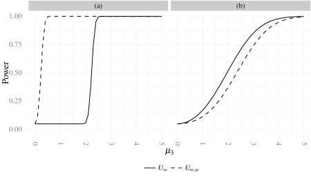
Figure 1: Power curves as a function of $\mu_{3}$ for the alternative model $X_{i}\sim N(\mu_{i},\sigma_{i}^{2})$ with $\mu_{1}=\mu_{2}=0$ and $\mu_{3}>0$ against the null hypothesis that $\mu_{i}=0$ for all $i=1,2,3$. The standard deviations are (a) $\sigma_{1}=\sigma_{2}=1$ and $\sigma_{3}=0.1$, (b) $\sigma_{1}=\sigma_{2}=0.1$ and $\sigma_{3}=1$. The lines represent the tests based on the deviation measures $U_{\infty}$ (unscaled test) and $U_{\infty,w}$ (scaled test). See the text for details.

3.4.  Asymmetric distribution of residuals

Sometimes the distribution of the residuals (under the null model) may be clearly asymmetric around $T_{0}(r)$. Then transformations making the distribution more symmetric are helpful. A simple directional scaling which treats negative and positive residuals differently, is

$$d_{\text{qdir}}(r)=\mathbf{1}(d(r)\geq 0)\frac{d(r)}{|\overline{T}(r)-T_{0}(r)|}+\mathbf{1}(d(r)<0)\frac{d(r)}{|\underline{T}(r)-T_{0}(r)|}.$$ (6)

The directional quantile scaling (6) utilises as (5) the quantiles $\underline{T}(r)$ and $\overline{T}(r)$, to weigh negative and positive residuals, and, furthermore, as (5) it makes the variances of residuals more uniform for the different distances $r$. The following toy example demonstrates that severe asymmetry should be removed, if there is no a priori interesting direction of deviation from $T_{0}(r)$.

Toy example 2. The random variables $X_{i}$ have asymmetric distributions with distribution functions

$$F_{X_{i}}(x;\mu_{i},\sigma_{ai}^{2},\sigma_{bi}^{2})=\frac{1}{2}F_{a}(x;\mu_{i},\sigma_{ai}^{2})+\frac{1}{2}F_{b}(x;\mu_{i},\sigma_{bi}^{2}),$$ (7)

where $F_{a}$ is the distribution function of the truncated normal distribution on $[\mu_{i}.\infty)$ and $F_{b}$ is the distribution function for $(-\infty,\mu_{i})$. The variances $\sigma_{ai}^{2}$ and $\sigma_{bi}^{2}$ are assumed to be known. If $\sigma_{ai}>\sigma_{bi}$ the fatter tail of the distribution of $X_{i}$ lies right from $\mu_{i}$.

The null and alternative hypotheses are as in Toy example 1. Now the power of the tests based on $U_{\infty}=\max_{i}|X_{i}|$ and $U_{\infty,w}=\max_{i}\left(\mathbf{1}\left(X_{i}\geq 0\right)|X_{i}|/a_{1i}+\mathbf{1}\left(X_{i}<0\right)|X_{i}|/a_{2i}\right)$ are compared. Again this can be carried out analytically, see the Appendix.

If $\sigma_{ai}<\sigma_{bi}$, the unscaled test has difficulties to observe the positive deviation of $\mu_{3}$ from zero and has therefore smaller power than the scaled test, see Figure 2 (a). On the other hand, for $\sigma_{ai}>\sigma_{bi}$ the scaling (6) is counter productive, see Figure 2 (b).

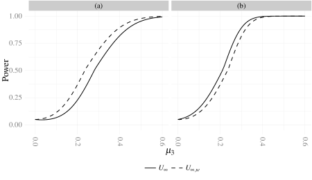
Figure 2: Power curves as a function of $\mu_{3}$ for the alternative model $X_{i}\sim$(7) with $\mu_{1}=\mu_{2}=0$ and $\mu_{3}>0$ against the null hypothesis that $\mu_{i}=0$ for all $i=1,2,3$. The standard deviations in (7) are $\sigma_{ai}=0.1$ and $\sigma_{bi}=c\sigma_{ai}$ for all $i=1,2,3$ with (a) $c=1.3$, (b) $c=0.7$. The lines represent the tests based on the deviation measures $U_{\infty}$ (unscaled test) and $U_{\infty,w}$ (scaled test). See the text for details.

4.  Simulation study design

In order to be concrete, we now consider an important particular case: testing of the random labelling hypothesis for marked point patterns with non-negative real-valued marks. The assumption is that the marked pattern can be thought to be generated in two steps: first generating the points and then labelling the points independently with marks following some mark distribution. The corresponding point process can be stationary, non-stationary or finite; the test is carried out conditionally to the (unmarked) point pattern and, thus, all these cases are treated identically.

As test functions $T(r)$ we use functions which are closely related to the mark-weighted $K$-functions as defined for stationary marked point processes in Penttinen and Stoyan (1989) and Illian et al. (2008). These functions are natural generalisations of Ripley’s $K$-function. We explain them first for the stationary case.

4.1.  Mark-weighted $K$-functions

It is well known that Ripley’s $K$-function can be explained as follows: $\lambda K(r)$ is the mean number of other points within distance $r$ from a typical point of the process, i.e. $\lambda K(r)=\mathbb{E}_{o}\left(\sum_{x\in N}\mathbf{1}_{b(o,r)}(x)\right)$, where the expectation is with respect to the Palm distribution and $b(o,r)$ denotes the disc with radius $r$ centred at $o$ (Ripley 1976, 1977).

The mark-weighted $K$-function (Penttinen and Stoyan 1989; Illian et al. 2008), $K_{f}(r)$, has a similar form as $K(r)$, but it also takes the marks into account through a mark test function $f(m_{1},m_{2}):\mathbb{R}^{2}\rightarrow\mathbb{R_{+}}$. It is

$$\lambda K_{f}(r)=\left.\mathbb{E}_{o}\left(\sum_{[x;\,m(x)]\in N_{m}}f(m(o),m(x))\mathbf{1}_{b(o,r)}(x)\right)\right/c_{f},$$

where

$$c_{f}=\int_{0}^{\infty}\int_{0}^{\infty}f(m_{1},m_{2})F_{M}(\text{d}m_{1})F_{M}(\text{d}m_{2}),$$ (8)

is a normalising factor, which depends on the test function $f$. In (8), $F_{M}(m)$ is the mark distribution function. In the case of independent marking it holds

$$K_{f}(r)=K(r),\quad r\geq 0,$$ (9)

see Penttinen and Stoyan (1989).

There are various possibilities for choosing the mark test function $f$ (see e.g. Schlather 2001; Illian et al. 2008). Table 1 lists the $K_{f}$ functions that are used in this paper, together with the corresponding $f$ and $c_{f}$.

The mark test functions in Table 1 look at mark behaviour from different points of view. The function $K_{m.}$ explores the mark value given that there is a further point within distance $r$. This function may be used for detecting dependencies between marks and points (Schlather et al. 2004; Guan 2005). The function $K_{mm}(r)$ is based on products of marks of point pairs of distance $r$. It is useful e.g. in situations where the marks have the tendency to be smaller than the mean mark for points close together. In contrast, $K_{\gamma}(r)$ is based on mark differences and helps to detect situations where the marks of points close together tend to be similar. Thus the choice of $K_{f}$-functions for the test should be determined by knowledge of the patten.

Summary	$f(m_{1},m_{2})$	$c_{f}$
$K_{m.}(r)$	$m_{1}$	$\mu_{m}$
$K_{mm}(r)$	$m_{1}m_{2}$	$\mu_{m}^{2}$
$K_{\gamma}(r)$	$\frac{1}{2}(m_{1}-m_{2})^{2}$	$\sigma_{m}^{2}$

Table 1: Different $K_{f}$-functions, their mark test functions $f(m_{1},m_{2})$ and normalising factors $c_{f}$.

The estimation of the $K_{f}$-functions in the stationary case is carried out similarly as that of the $K$-function. Let $n$ be the number of points of the analysed marked point pattern observed in the window $W$ with area $|W|$. Then the $K_{f}$-function can be estimated as

$$\hat{K}_{f}(r)=\frac{1}{|W|\widehat{\lambda^{2}}\hat{c}_{f}}\sum_{k=1}^{n}\sum_{l=1,l\neq k}^{n}f\left(m(x_{k}),m(x_{l})\right)\mathbf{1}\left(||\,x_{k}-x_{l}||\leq r\right)e(x_{k},x_{l}),$$ (10)

where $e(x_{k},x_{l})$ is an edge-correction factor and

$$\widehat{\lambda^{2}}=n(n-1)/|W|^{2}\quad\text{and}\quad\hat{c}_{f}=\sum_{i=1}^{n}\sum_{j=1,j\neq i}^{n}f(m(x_{i}),m(x_{j}))/n(n-1)$$ (11)

are estimators of $\lambda^{2}$ and $c_{f}$, see Illian et al. (2008). For the translational edge-correction, the edge-correction factor is $e(x_{k},x_{l})=|W|/|W_{x_{k}}\cap W_{x_{l}}|$, where $|W_{x_{k}}\cap W_{x_{l}}|$ is the area of the intersection of $W_{x_{k}}$ and $W_{x_{l}}$, and $W_{x}$ is the translated window $W_{x}=\{s+x,\,s\in W\}$ (see Illian et al. 2008, p. 353). For the case of “no edge-correction”, it is simply $e(x_{k},x_{l})\equiv 1$.

Remark. The estimator $\hat{c}_{f}$ in (11) differs in one point from the estimator given in Illian et al. (2008, p. 353): the estimator (11) is adapted to a marking in $W$ where the marks of the $n$ points in $W$ are given to the points by random permutation. This leads to the simple equation (12) below. Note that in neither case $\hat{K}_{f}(r)$ is an unbiased estimator of $K_{f}(r)$, because of the division by $\hat{c}_{f}$ and $\widehat{\lambda^{2}}$.

4.2.  The test procedure

The random labelling hypothesis is tested as follows. Suppose a marked point pattern $\{[x_{1},m(x_{1})],\ldots,[x_{n},m(x_{n})]\}$ of $n$ points is observed in the window $W$. For this pattern the function $\hat{K}_{f}(r)$ is determined by (10). The result $\hat{K}_{f,1}(r)$ is compared with further functions $\hat{K}_{f,i}(r)$ determined for $s$ simulated marked point patterns. For all simulations the points are fixed, while the original marks $m(x_{i})$ are randomly permuted. Thus $\hat{K}_{f}(r)$ plays the role of $T(r)$.

The expectation of $\hat{K}_{f}(r)$ under the null model of random permutation of the marks is simply $\hat{K}(r)$, since even $\hat{c}_{f}$ is fixed in (10) and only the $m(x_{k})$ and $m(x_{l})$ are variable. This means that

$$T_{0}(r)=\hat{K}(r),$$ (12)

where $\hat{K}(r)$ is obtained by (10) with $f\equiv 1$. Note that this equation holds true for all forms of estimators of $K$ and $K_{f}$ as long as the same form of edge-correction, e.g. translational, Ripley’s or “no correction”, is used for $\hat{K}$ and $\hat{K}_{f}$. Of course, the numerical values differ. Note that all is conditional on the fixed points in the window $W$, which implies that the test can be used also for non-stationary or finite point processes.

To conduct the test, the residuals and global deviation measures are then determined. In the following simulation study the effects of transformation, scaling etc. are investigated.

4.3.  Alternative models

For our power comparison we use four marked point process models with different forms of mark correlations. The first process is finite while the other three processes are stationary.

4.3.1.  Sequential neighbour-interaction marked point process

The sequential neighbour-interaction marked point process (SeqNIMPP) can be thought of as a generalisation of Diggle’s simple sequential inhibition model known also as the random sequential absorption (RSA) process (see e.g. Penrose and Shcherbakov 2009). It is also related to the multivariate point process with hierarchical interactions studied in Grabarnik and Särkkä (2009), who applied their model to an analysis of the spatial structure of a forest stand. The SeqNIMPP model is a finite point process in $W$.

A realization in a bounded window $W$ can be constructed as follows: Denote the marked point with location $x$ and mark $m$ as $y=[x,m]$. Assuming that the marks of the marked points $y_{1},y_{2},\ldots y_{n}$ are known, the corresponding locations are allocated sequentially in $W$. The location $x_{1}$ of the first point $y_{1}$ has uniform distribution over $W$, while the location of the $k$th point follows the conditional density

$$f_{k}([x_{k},m_{k}]\;|\;y_{k-1},\ldots,y_{1})=\frac{\exp\left\{-U_{k}([x_{k},m_{k}];\;y_{\leq k-1})\right\}}{\int_{W}\exp\left\{-U_{k}([x,m_{k}];\;y_{\leq k-1})\right\}\text{d}x},$$

where $U_{k}(y_{k};y_{\leq k-1})=\sum_{i=1}^{k-1}I(y_{i},y_{k})$. The quantity $U_{k}$ can be interpreted as the impact of the previously allocated points $y_{\leq k-1}=(y_{1},\ldots,y_{k-1})$ on the point $y_{k}=[x_{k},m_{k}]$, where $I(y_{i},y_{k})$ models the influence of the earlier point $y_{i}$ on the point $y_{k}$.

We assume that the marks stem from a Gaussian distribution with mean $\mu$ and variance $\sigma^{2}$, truncated to avoid negative marks, and use the influence function

$$I(z,y)=\theta{\bf 1}\left(\|z-y\|<R\,m(z)/\mu\right)\frac{m(z)m(y)}{(\mu/R)^{2}\|z-y\|}.$$

Here $m(z)$ is the mark of point $z$, $\theta$ is a parameter controlling the strength of influence and $R$ is an interaction radius. If $\theta$ is positive, then the points tend to avoid positions in the neighbourhood of previously allocated points, the more the larger the marks of the previously allocated points are. Further, the mark of the point itself matters; the larger it is, the less likely it is for it to appear close to a previously allocated point. If $\theta$ is negative, on the other hand, then points attract new points, and the degree of attraction depends on the marks of the new and the previously allocated points. The case $\theta=0$ corresponds to “no interaction between points”, i.e. independent marks.

4.3.2.  Exponential intensity-marked Cox process

While the SeqNIMPP model creates regular patterns with inhibition between points (for $\theta>0$), the stationary exponential intensity-marked Cox process (ExpCP) introduced by Myllymäki and Penttinen (2009) forms clustered patterns of points. The points stem from a log Gaussian Cox process (LGCP) $N=\{x_{i}\}$ with random intensity $\Lambda(s)=\exp(Z(s))$, where $\{Z(s)\}$ is a stationary Gaussian random field. It has mean $\mu_{Z}$ and the special covariance function $C_{Z}(r)=\exp(-r/\phi_{Z})$, where $\phi_{Z}$ is a range parameter. Conditional on the random intensity the marks are distributed as

$$m(x_{i})|\Lambda(x_{i})\sim\text{Exp}\Big{(}1/(a+b/\Lambda(x_{i}))\Big{)}\quad\text{(ExpNIMCP)}$$ (13)

with expectation $\mathbb{E}(m(x_{i})|\Lambda(x_{i}))=a+b/\Lambda(x_{i})$, or by

$$m(x_{i})|\Lambda(x_{i})\sim\text{Exp}\Big{(}1/(a+b\Lambda(x_{i}))\Big{)}\quad\text{(ExpPIMCP)}$$ (14)

with expectation $\mathbb{E}(m(x_{i})|\Lambda(x_{i}))=a+b\Lambda(x_{i})$, where $a$ and $b$ are positive model parameters. In these models both the mean and variance of marks depend on the local point density: In the ExpNIMCP model, the marks tend to be small and less variable in areas with high intensity, while in low intensity areas both small and large marks can occur. In the ExpPIMCP model, on the other hand, mean and variance of marks tend to be large in high intensity areas. For more details see Myllymäki and Penttinen (2009) and Myllymäki (2009), where the model (13) was applied to model structure of rainforest data.

4.3.3.  Gaussian noise intensity-marked Cox process

The Gaussian noise intensity-marked Cox process (GNIMCP) is similar to the ExpIMCP model and the models considered in Ho and Stoyan (2008). The points stem from the same LGCP model with the intensity $\Lambda(s)=\exp(Z(s))$ as the points in the ExpIMCP model, and the marks are

$$m(x_{i})=a\cdot\exp\left\{b\left(\frac{Z^{*}(x_{i})-\mu_{Z}}{1+\sigma_{\epsilon}}\right)\right\},$$

where $a$ and $b$ are real mark-scale parameters and $\mu_{Z}$ is the mean of $Z$. The strength of dependence between marks and points is controlled through $Z^{*}$: $Z^{*}(x_{i})=Z(x_{i})+\epsilon(x_{i})$, where $\epsilon(x_{i})\sim N(0,\sigma_{\epsilon}^{2})$ are i.i.d. The larger the variance $\sigma_{\epsilon}^{2}$ is, the noisier the values of $Z^{*}$ and marks are.

If the parameter $b$ is positive (negative), then the marks in high intensity areas tend to be larger (smaller) than in low intensity areas. The distribution of $m(x_{i})$ given $Z(x_{i})$ is lognormal.

4.3.4.  A random field model: Gaussian noise Cox process

Again, the points come from the LGCP model. The Gaussian noise Cox process (GNCP) is a particular case of the random field model, see Illian et al. (2008), since the marks are generated as follows: To mimic the GNIMCP model, let $\{Z_{M}(s)\}$ be an independent Gaussian random field with mean $\mu_{Z}$ and covariance function $C_{Z}(r)=\exp(-r/\phi_{Z})$, and define $Z_{M}^{*}(s)=Z_{M}(s)+\epsilon(s)$ and

$$U(s)=a\cdot\exp\left\{b\left(\frac{Z_{M}^{*}(s)-\mu_{Z}}{1+\sigma_{\epsilon}}\right)\right\},$$

where $a$ and $b$ are model parameters and $\epsilon(s)\sim N(0,\sigma_{\epsilon}^{2})$. Then the marks are simply $m(x_{i})=U(x_{i})$.

In this model, there is no relationship between local point density and marks, but points close together tend to have similar marks. This similarity of marks decreases when the variance $\sigma_{\epsilon}^{2}$ increases.

5.  Power comparison by the simulation study

In order to observe how the ingredients of the random labelling test affect its power, we tested the random labelling hypothesis against the four alternative marked point process models in Section 4.3 with various parameter combinations summarised in Table 2. In each model, one of the parameters (called the “changing parameter”) controlling the strength of spatial correlations has been selected and is systematically varied, while the other, fixed parameters have been chosen such that the most prominent deviation of $T(r)$ from $T_{0}(r)$ occurs approximately at the distance $r=6$ (determined by simulation).

Model	Fixed mark parameters	Changing parameter
SeqNIMPP	$\mu=24$, $\sigma^{2}=9$	$\theta=0,0.02,0.04,\dots,0.20$
ExpNIMCP (13)	$b=1$	$a=0,20,40,\dots,200$
ExpPIMCP (14)	$b=6600$	$a=0,250,500,\dots,2500$
GNIMCP, $b<0$	$a=24$, $b=-0.12$	$\sigma_{\epsilon}=0,0.5,1.0,\dots,6.0$
GNIMCP, $b>0$	$a=24$, $b=0.12$	$\sigma_{\epsilon}=0,0.5,1.0,\dots,6.0$
GNCP	$a=24$, $b=-0.12$	$\sigma_{\epsilon}=0,0.25,0.5,\dots,3.5$

Table 2: Parameter values of the SeqNIMPP (see Section 4.3.1), ExpIMCP (Section 4.3.2), GNIMCP (Section 4.3.3) and GNCP (Section 4.3.4) models used in the simulation experiment. As the mean and range of correlation parameters of the LGCP models we used $\mu_{Z}=-4.4$ and $\phi_{Z}=4$, respectively.

For each model we made $N=1000$ simulations with $n=200$ points in a window of size $[0,100]\times[0,100]$. For each simulated marked point pattern, we performed tests based on $s=999$ random permutations of marks. The tests were made with

1. $T(r)=\hat{K}_{f}(r)$ ((10) with the translational edge correction) with the mark test functions $f$ given in Table 1,

2. the transformation $h(\cdot)=\sqrt{\cdot/\pi}$,

3. raw (1), studentised (4), quantile (5) and directional quantile (6) residuals,

4. deviation measures (2) and (3), and

5. three intervals $I$ of $r$-values: $I_{1}=[4,8]$, $I_{2}=[3,15]$ and $I_{3}=[0,25]$.

All alternatives in (iii)-(v) were considered both for the test function $T(r)=\hat{K}_{f}(r)$, and its transformation $\hat{L}_{f}(r)=\sqrt{\hat{K}_{f}(r)/\pi}$. The three intervals $I$ were chosen to separate effects which could influence the power in the comparative study.

We argue that a fair comparison between different forms of the deviation test can be done only if the distributions of residuals are approximately uniform. Therefore, we first compare the different mark test functions based on the shortest interval $I_{1}$, in order to eliminate effects of the other factors, and choose the most powerful mark test function for each model, which will be used in other comparisons. We then use the widest interval $I_{3}$ for comparing (ii)-(iii), and also (iv) after scalings, while $I_{2}$ is used to study the effects of the width of $I$.

The number of simulated patterns for which the null hypothesis is rejected among the $N$ simulations gives an estimate for the power. The results below are for the significance level 0.05.

5.1.  Comparison of mark test functions

As said above, to compare different mark test functions, the attention is restricted to the narrow interval $I_{1}=[4,8]$. Since the contributions of raw residuals of $\hat{K}_{f}(r)$ for different $r$ are approximately equal on $I_{1}$, the test based on these residuals can be used without any transformations or scalings. On this narrow interval, also differences between the deviation measures (2) and (3) are negligible and, thus, Figure 3 shows the results only for (2). The power for the various summary functions $\hat{K}_{f}$ (or mark test functions $f$) depends on the alternative model:

1. The function $\hat{K}_{m.}$ leads to powers at least as high as for any other function for the SeqNIMPP, ExpNIMCP and GNIMCP models, while, for the random field model GNCP, its power is low. For the ExpPIMCP model, the power related to $\hat{K}_{m.}$ is slightly lower than that for $\hat{K}_{mm}$.

2. The function $\hat{K}_{mm}$ is approximately as powerful as $\hat{K}_{m.}$ for the SeqNIMPP, ExpPIMCP and GNIMCP models, where the marks tend to be either smaller or larger (depending on model parameters) than the mean mark for points close together. On the other hand, in the ExpNIMCP model, the marks at points close together are not clearly smaller than the mean mark and, therefore, $\hat{K}_{mm}$ does not have high power. For the GNCP model, the power is similarly low.

3. The function $\hat{K}_{\gamma}$ leads to a powerful test for the GNCP model, because of its sensibility to similar marks at short distances. Note that the marks of points close together also tend to be similar also in the GNIMCP models, but for these models $\hat{K}_{m.}$ and $\hat{K}_{mm}$ lead to much more powerful test than $\hat{K}_{\gamma}$ for the reasons explained above.

We conclude that indeed the power of deviation test depends on the choice of the summary function, which should be adapted to the alternative model.

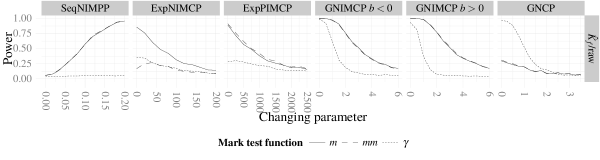
Figure 3: Power comparison of the $\hat{K}_{f}$ functions with different mark test functions $f(m_{1},m_{2})$ for the models of Table 2 (top panel) using the test based on the supremum deviation measure (2) applied to the raw residuals of $\hat{K}_{f}(r)$ on $I_{1}=[4,8]$.

5.2.  Comparison of transformations and scalings

5.2.1.  Transformation

The square root transformation increases greatly the power for all the alternative models, as it is seen from the power curves of the tests based on raw residuals of $\hat{K}_{f}(r)$ and $\hat{L}_{f}(r)$ in Figure 4. The reason for the increase in power is that the residuals of $\hat{L}_{f}(r)$ are more uniform than those of $\hat{K}_{f}(r)$.

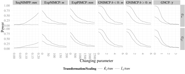
Figure 4: Power comparison of square root transformation for the models of Table 2 with the most powerful mark test functions $f$ (top panel) using the deviation measures (2) and (3) (right panel) applied to the raw residuals of $\hat{K}_{f}(r)$ and $\hat{L}_{f}(r)$ on $I_{3}=[0,25]$.

5.2.2.  Scaling

Figures 5 and 6 show power curves for the deviation measures (2) and (3) applied to the raw (1), studentised (4), quantile (5) and directional quantile (6) residuals of the test function $T(r)=\hat{K}_{f}(r)$ and its transformation $\hat{L}_{f}(r)$, respectively. We found the following:

1. Always the power of the tests based on raw residuals is lowest.

2. The results with the studentised (4) and quantile (5) scalings are very similar.

3. For the ExpNIMCP and GNCP models (for the latter only for $\hat{K}_{f}(r)$), the directional scaling (6) improves further the power, while for the ExpPIMCP the scaling (6) is counter productive. The problem of asymmetry plays a role for these models: The ExpIMCP models have an asymmetric mark distribution, and we found that also the empirical distributions of residuals are asymmetric. Moreover, we found that the residual distributions are more asymmetric for $\hat{K}_{\gamma}$ than for $\hat{K}_{m.}$ and $\hat{K}_{mm}$, which explains the result for the GNCP model.

Note that the improvements of power by scalings are smaller for $\hat{L}_{f}(r)$ than for $\hat{K}_{f}(r)$, since the residuals of the transformed test function are more uniform than the raw residuals.

Figure 5: Power comparison of scalings (raw; studentised ’st’, quantile ’q’ and directional quantile ’qdir’) for the models of Table 2 with the most powerful mark test functions $f$ (top panel) using the deviation measures (2) and (3) (right panel) applied to the different residuals of $\hat{K}_{f}(r)$ on $I_{3}=[0,25]$.

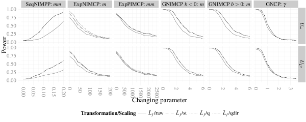
Figure 6: Power comparison of scalings (raw; studentised ’st’, quantile ’q’ and directional quantile ’qdir’) for the models of Table 2 with the most powerful mark test functions $f$ (top panel) using the deviation measures (2) and (3) (right panel) applied to the different residuals of $\hat{L}_{f}(r)$ on $I_{3}=[0,25]$.

5.2.3.  Combined transformation and scaling

Figure 7 compares the tests based on the scaled residuals of $\hat{K}_{f}$ to those of $\hat{L}_{f}$. We observe the following:

1. For the SeqNIMPP and GNIMCP models, the differences between the powers of the tests based on scaled residuals of $\hat{K}_{f}(r)$ or $\hat{L}_{f}(r)$ are very small, and these tests have clearly higher power than the test based on the raw residuals of the transformed test function $\hat{L}_{f}(r)$.

2. For the ExpNIMCP and GNCP models, the power for the test based on the quantile residuals (5) of $\hat{K}_{f}(r)$ is lower than for the test based on the corresponding residuals of $\hat{L}_{f}(r)$ (and, for the measure (2), even lower than for the test based on raw residuals of $\hat{L}_{f}$). For the ExpPIMCP model, the opposite occurs for the measure (3).

3. Similarly, applying first the square root transformation and then the scaling (6) results in more powerful tests than applying pure scaling (6) to $\hat{K}_{f}(r)$ for the ExpNIMCP and GNCP models, and the other way around for the ExpPIMCP model.

4. For the GNCP model, the scaling (6) has no advantage over the scaling (5) if the transformation is employed first.

The result 1 above indicates that the transformation, prior to scaling, is unnecessary for the SeqNIMPP and GNIMCP models, whereas the results 2-3 show that it is useful in the case of the ExpNIMCP and GNCP models. As pointed out already above, for the latter models the asymmetry plays a role. Clearly the scalings (5) and (4) do not decrease asymmetry in the distribution of the residuals, but, in this particular case, it appears that the square root transformation does, as does the scaling (6).

Thus, a transformation can lead to a change in the form of the distribution of residuals. In general, it can reduce as well as induce asymmetry. However, typically it will not make the distribution of residuals completely uniform for all distances on $I$ and scalings lead to further improvements in power, see Figures 6 and 7. We conclude that a good strategy appears to be to use a suitable transformation, if available, and then scaling to further reduce inhomogeneity of residuals.

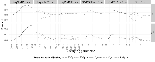
Figure 7: Power comparison of the square root transformation and scalings (raw; studentised ’st’, quantile ’q’ and directional quantile ’qdir’) for the models of Table 2 with the most powerful mark test functions (top panel) using the deviation measures (2) and (3) (right panel) on $I_{3}=[0,25]$. The curves show the power difference with respect to the power of the test based on raw residuals of $\hat{L}_{f}$ (represented by the zero line).

5.3.  Comparison of deviation measures

Figure 8 shows results with the supremum (2) and integral (3) deviation measures applied to the scaled residuals (6) of $\hat{L}_{f}$ on the range of distances $I_{3}=[0,25]$. For the SeqNIMPP model, for which the deviance from the null model is reasonably sharp, the supremum measure leads to a clearly higher power than the integral measure. For the other models, the measures (2) and (3) lead approximately to the same power and, thus, do not play an important role.

Figure 8: Power comparison of the supremum $U_{\infty}$ (2) and integral $U_{L^{2}}$ (3) deviation measures applied to the residuals (6) of $\hat{L}_{f}$ on $I_{3}=[0,25]$ for the models of Table 2 with the most powerful mark test functions (top panel).

5.4.  Range of distances and scaling

There is some balance between the length of the interval $I$ and scaling. Figure 9 shows powers for tests with different intervals $I$. The powers of the tests based on raw residuals of $\hat{K}_{f}$ as well as for $\hat{L}_{f}$ are highly increased from $I_{3}$ to $I_{2}$ and from $I_{2}$ to $I_{1}$. However, for the tests based on scaled residuals we observe hardly any increase in power from $I_{3}$ and $I_{2}$ to $I_{1}$.

In general, the shorter the interval $I$, the more powerful the test can be as long as the interesting behavior occurs inside $I$. However, as the results in Figure 9 show, if appropriate transformations and scalings are used, there is only a weak relationship between the power and the length of $I$. However, for the SeqNIMPP model, the non-powerful deviation measure (3) is still clearly more powerful on $I_{1}$ than on $I_{2}$ and $I_{3}$ (figure not shown).

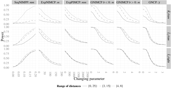
Figure 9: Power comparison of the intervals of distances $I_{3}=[0,25]$, $I_{2}=[3,15]$ and $I_{1}=[4,8]$ for the models of Table 2 with the most powerful mark test functions (top panel) using the supremum deviation measure (2) applied to the raw residuals of $\hat{K}_{f}$ and $\hat{L}_{f}$ and scaled residuals (6) of $\hat{L}_{f}$ (right panel).

At the end of this section we mention briefly the two further results. The first concerns the problem of edge-correction. As discussed already, the estimator (10) stems from the stationary process context. In the random labelling test there is no need of edge-correction since we deal with a fixed point pattern in the bounded window $W$. So we also made the tests on $I_{3}$ for the processes in Table 2 without edge-correction (i.e. $e(x_{k},x_{l})=1$) and observed that the power was a little higher than for the estimator with edge-correction if no scalings were used.

We also made a corresponding simulation experiment as reported above based on $n=800$ points in a window of size $[0,200]\times[0,200]$. The results with $n=800$ were analogous to those with $n=200$, except the values of power were larger, showing the consistency property empirically.

6.  Discussion and conclusions

This paper considers the construction of deviation tests for point processes in a general form. The tests are applicable also for non-stationary and finite point processes, since they are based on a test function and its expectation under the null hypothesis, which can be estimated from simulations from the null model if it is not known analytically. Thus, there is no need to assume stationarity and to use unbiased estimators of summary functions in the test. The paper demonstrates the tests for finite and stationary point processes in the case of the random labelling hypothesis.

The main point in constructing a powerful deviation test is to choose a suitable test function $T(r)$. For the random labelling test we used mark-weighted $K$ functions, where the choice of the mark test function $f$ is essential. Which mark test functions will lead to the most powerful test depends on properties of the point pattern under analysis. If a researcher has an alternative model in mind, this model may suggest the mark test function to be used.

When the test function $T(r)$ is chosen, the next problem is search for a suitable transformation. The simulation study shows that transformations of summary functions can increase the power of deviation tests, since they allow to make the distribution of residuals more uniform over distances. There are some classical transformations, and perhaps new transformations can be developed.

Finally, scalings of residuals can further improve the power of tests based on transformed summary functions, because they lead to approximately even variances of residuals for different distances, unlike transformation only. While transformations may reduce or induce asymmetry in the distribution of residuals, scaling is a simple way to make distributions of residuals more uniform. As shown by the simulation study, scalings also act in some form of balance with the choice of the length of the interval $I$, i.e. an appropriate scaling can make the choice of $I$ unimportant.

In some sense, the role of transformations and scalings is similar to that of prior distributions in Bayesian statistics. If there is not an a priori interesting distance $r$, then it makes sense to give similar importance to all residuals in the chosen interval of distances $I$. Thus, the residual distributions for different distances should be made uniform, which, in the context of deviation tests, can be done by means of transformations and scalings. As the toy examples and the simulation study demonstrated, such transformations and scalings typically, but not necessarily, improve the power of the deviation test.

Appendix: The power in the toy examples

A.1 Toy example 1

Let $X_{i}\sim N(\mu_{i},\sigma_{i}^{2})$, $i=1,\dots,n$, $U_{\infty}=\max_{i}|X_{i}|$ and $U_{\infty,w}=\max_{i}(w_{i}|X_{i}|)$ with $w_{i}=1/\sigma_{i}$. Then $Y_{i}=|X_{i}|$ follows the folded normal distribution with cumulative distribution function

$$F_{Y_{i}}(y;\mu_{i},\sigma_{i}^{2})=\Phi\left(\frac{y-\mu_{i}}{\sigma_{i}}\right)+\Phi\left(\frac{y+\mu_{i}}{\sigma_{i}}\right),\quad y\geq 0,$$ (15)

where $\Phi(\cdot)$ is the cumulative distribution function of the standard normal distribution. Further, the distribution function of $U_{\infty}$ is

$$F_{U_{\infty}}(u;\mu_{1},\dots,\mu_{n},\sigma_{1},\dots,\sigma_{n}) = \mathbf{P}\left(\max_{i=1,\dots,n}Y_{i}\leq u\right)$$ (16)

$$= \prod_{i=1}^{n}P(Y_{i}\leq u)=\prod_{i=1}^{n}F_{Y_{i}}(u;\mu_{i},\sigma_{i}^{2}).$$

If $\mu_{i}=0$, the distribution (15) is called half-normal distribution and it simplifies to

$$F_{Y_{i}}(y,0,\sigma_{i}^{2})=\int_{0}^{y}\frac{1}{\sigma_{i}}\sqrt{\frac{2}{\pi}}\exp\left(-\frac{u^{2}}{2\sigma_{i}^{2}}\right)\text{d}u.$$

The critical value $c_{\text{crit}}$ for the null hypothesis that $\mu_{i}=0$ for all $i=1,\dots,n$ can be obtained by solving $F_{U_{\infty}}(c_{\text{crit}};0,\dots,0,\sigma_{1},\dots,\sigma_{n})=1-\alpha$, where $\alpha$ is the significance level and $F_{U_{\infty}}$ is given in (16). Thereafter the power of the unscaled test for the alternative hypothesis $H_{1}$: $\mu_{i}\neq 0$ for $i\in I_{1}$, where $I_{1}$ is a subset of $I=\{1,\dots,n\}$, can be obtained from

$$\mathbf{P}\left(\max_{i=1,\dots,n}|X_{i}|>c_{\text{crit}}\right)=1-F_{U_{\infty}}(c_{\text{crit}};\mu_{1},\dots,\mu_{n},\sigma_{1},\dots,\sigma_{n}).$$

The power of the scaled test can be obtained similarly, because for $Z_{i}=w_{i}Y_{i}=w_{i}|X_{i}|$ it holds

$$F_{Z_{i}}(u;\mu_{i},\sigma_{i}^{2})=\mathbf{P}(Z_{i}\leq u)=\mathbf{P}(Y_{i}\leq u/w_{i})=F_{Y_{i}}(u/w_{i},\mu_{i},\sigma_{i}^{2})$$

and the distribution of $U_{\infty,w}$ is

$$F_{U_{\infty,w}}(u;\mu_{1},\dots,\mu_{n},\sigma_{1},\dots,\sigma_{n})=\mathbf{1}\left(\max_{i=1,\dots,n}Z_{i}\leq u\right)=\prod_{i=1}^{n}F_{Z_{i}}(u,\mu_{i},\sigma_{i}^{2}).$$ (17)

A.2 Toy example 2

Assume the random variable $X_{i}$ has the distribution (7) and $Y_{i}=|X_{i}|$. Since $\mathbf{P}(Y_{i}\leq y)=\mathbf{P}(-y\leq X_{i}\leq y)$, the distribution of $Y_{i}$ is

$$F_{Y_{i}}(y;\mu_{i},\sigma_{ai}^{2},\sigma_{bi}^{2}) = F_{X_{i}}(y;\mu_{i},\sigma_{ai}^{2},\sigma_{bi}^{2})-F_{X_{i}}(-y;\mu_{i},\sigma_{ai}^{2},\sigma_{bi}^{2})$$

$$= \frac{1}{2}(F_{1}(y;\mu_{i},\sigma_{ai}^{2})-F_{1}(-y;\mu_{i},\sigma_{ai}^{2}))+$$

$$\frac{1}{2}(F_{2}(y;\mu_{i},\sigma_{bi}^{2})-F_{2}(-y;\mu_{i},\sigma_{bi}^{2})),$$

for $y>0$ (0 otherwise). Then the distribution of $U_{\infty}=\max_{i}Y_{i}$ is

$$F_{U_{\infty}}(u;\mu_{1},\dots,\mu_{n},\{\sigma_{ai},\sigma_{bi}\})=\prod_{i=1}^{n}F_{Y_{i}}(u;\mu_{i},\sigma_{ai}^{2},\sigma_{bi}^{2}),$$

similarly as (16). Let then $Z_{i}=\mathbf{1}(X_{i}\geq 0)w_{i}^{(+)}X_{i}+\mathbf{1}(X_{i}<0)w_{i}^{(-)}X_{i}$, where $w_{i}^{(+)}$ and $w_{i}^{(-)}$ are weights. The distribution of $Z_{i}$ is

$$F_{Z_{i}}(u;\mu_{i},\sigma_{ai}^{2},\sigma_{bi}^{2}) = \mathbf{P}(Z_{i}\leq u)$$

$$= \mathbf{P}\left(Z_{i}\leq u|X_{i}\geq 0\right)\mathbf{P}\left(X_{i}\geq 0\right)+\mathbf{P}\left(Z_{i}\leq u|X_{i}<0\right)\mathbf{P}\left(X_{i}<0\right)$$

$$= \mathbf{P}\left(Z_{i}\leq u\;\&\;X_{i}\geq 0\right)+\mathbf{P}\left(Z_{i}\leq u\;\&\;X_{i}<0\right)$$

$$= \mathbf{P}\left(0\leq X_{i}\leq u/w_{i}^{(+)}\right)+\mathbf{P}\left(-u/w_{i}^{(-)}\leq X_{i}\leq 0\right)$$

$$= F_{X_{i}}\left(u/w_{i}^{(+)};\mu_{i},\sigma_{ai}^{2},\sigma_{bi}^{2}\right)-F_{X_{i}}\left(-u/w_{i}^{(-)};\mu_{i},\sigma_{ai}^{2},\sigma_{bi}^{2}\right),$$

and the distribution of $U_{\infty,w}=\max_{i}Z_{i}$ is obtained similarly as (17):

$$F_{U_{\infty,w}}(u;\mu_{1},\dots,\mu_{n},\{\sigma_{ai},\sigma_{bi}\})=\prod_{i=1}^{n}F_{Z_{i}}(u;\mu_{i},\sigma_{ai}^{2},\sigma_{bi}^{2}).$$

The powers of the tests based on $U_{\infty}$ and $U_{\infty,w}$ can then be calculated in the same way as in the case of the Toy example 1 above. That is, for $U_{\infty,w}$, solve first the critical value $c_{\text{crit}}$ for the null hypothesis that $\mu_{i}=0$ for all $i$ from $F_{U_{\infty,w}}(c_{\text{crit}};0,\dots,0,\{\sigma_{ai},\sigma_{bi}\})=1-\alpha$, and then calculate $\mathbf{P}\left(\max_{i=1,\dots,n}Z_{i}>c_{\text{crit}}\right)=1-F_{U_{\infty},w}(c_{\text{crit}};\mu_{1},\dots,\mu_{n},\{\sigma_{ai},\sigma_{bi}\})$ for the alternative hypothesis with $\mu_{1},\dots,\mu_{n}$ where $\mu_{i}\neq 0$ for $i\in I_{1}\subseteq I$, and similarly for $U_{\infty}$.

REFERENCES

- Aitkin and Clayton (1980) Aitkin, M. and Clayton, D. (1980). The fitting of exponential, Weibull and extreme value distributions to complex censored survival data using glim. Applied Statistics 29, 156–163.
- Baddeley et al. (2000) Baddeley, A. J., Kerscher, M., Schladitz, K. and Scott, B. T. (2000). Estimating the function without edge correction. Stat. Neerl. 54, 315–328.
- Barnard (1963) Barnard, G. A. (1963). Discussion of professor Bartlett’s paper. J. R. Stat. Soc. Ser. B Stat. Methodol. 25, 294.
- Besag and Diggle (1977) Besag, J. and Diggle, P. J. (1977). Simple Monte Carlo tests for spatial pattern. J. R. Stat. Soc. Ser. C. Appl. Stat. 26, 327–333.
- Besag (1977) Besag, J. E. (1977). Comment on ‘Modelling spatial patterns’ by B. D. Ripley. J. R. Stat. Soc. Ser. B. Stat. Methodol. 39, 193–195.
- Bretz et al. (2010) Bretz, F., Hothorn, T. and Westfall, P. (2010). Multiple comparisons using R. Chapman and Hall/CRC, 1st edn.
- Cressie (1993) Cressie, N. A. C. (1993). Statistics for spatial data, revised edn. Wiley, New York.
- Diggle (1979) Diggle, P. J. (1979). On parameter estimation and goodness-of-fit testing for spatial point patterns. Biometrics 35, 87–101.
- Diggle (2003) Diggle, P. J. (2003). Statistical analysis of spatial point patterns, 2nd edn. Arnold, London.
- Gignoux et al. (1999) Gignoux, J., Duby, C. and Barot, S. (1999). Comparing the performances of Diggle’s tests of spatial randomness for small samples with and without edge-effect correction: Application to ecological data. Biometrics 55, 156–164.
- Grabarnik and Chiu (2002) Grabarnik, P. and Chiu, S. N. (2002). Goodness-of-fit test for complete spatial randomness against mixtures of regular and clustered spatial point processes. Biometrika 89, 411–421.
- Grabarnik et al. (2011) Grabarnik, P., Myllymäki, M. and Stoyan, D. (2011). Correct testing of mark independence for marked point patterns. Ecological Modelling 222, 3888–3894.
- Grabarnik and Särkkä (2009) Grabarnik, P. and Särkkä, A. (2009). Modelling the spatial structure of forest stands by multivariate point processes with hierarchical interactions. Ecological Modelling 220, 1232–1240.
- Guan (2005) Guan, Y. (2005). Tests for independence between marks and points of a marked point process. Biometrics 62, 126–134.
- Ho and Chiu (2006) Ho, L. P. and Chiu, S. N. (2006). Testing the complete spatial randomness by Diggle’s test without an arbitrary upper limit. J. Stat. Comput. Simul. 76, 585–591.
- Ho and Chiu (2009) Ho, L. P. and Chiu, S. N. (2009). Using weight functions in spatial point pattern analysis with application to plant ecology data. Comm. Statist. Simulation Comput. 38, 269–287.
- Ho and Stoyan (2008) Ho, L. P. and Stoyan, D. (2008). Modelling marked point patterns by intensity-marked Cox processes. Statist. Probab. Lett. 78, 1194–1199.
- Illian et al. (2008) Illian, J., Penttinen, A., Stoyan, H. and Stoyan, D. (2008). Statistical analysis and modelling of spatial point patterns. John Wiley & Sons, Ltd, Chichester.
- Loosmore and Ford (2006) Loosmore, N. B. and Ford, E. D. (2006). Statistical inference using the G or K point pattern spatial statistics. Ecology 87, 1925–1931.
- Møller and Berthelsen (2012) Møller, J. and Berthelsen, K. K. (2012). Transforming spatial point processes into Poisson processes using random superposition. Adv. in Appl. Probab. 44, 42–62.
- Myllymäki (2009) Myllymäki, M. (2009). Statistical models and inference for spatial point patterns with intensity-dependent marks. Ph.D. thesis, University of Jyväskylä, Jyväskylä.
- Myllymäki and Penttinen (2009) Myllymäki, M. and Penttinen, A. (2009). Conditionally heteroscedastic intensity-dependent marking of log Gaussian Cox processes. Stat. Neerl. 63, 450–473.
- Penrose and Shcherbakov (2009) Penrose, M. D. and Shcherbakov, V. (2009). Maximum likelihood estimation for cooperative sequential adsorption. Adv. in Appl. Probab. 41, 978–1001.
- Penttinen and Stoyan (1989) Penttinen, A. and Stoyan, D. (1989). Statistical analysis for a class of line segment processes. Scand. J. Stat. 16, 153–168.
- Ripley (1976) Ripley, B. D. (1976). The second-order analysis of stationary point processes. J. Appl. Probab. 13, 255–266.
- Ripley (1977) Ripley, B. D. (1977). Modelling spatial patterns. J. R. Stat. Soc. Ser. B Stat. Methodol. 39, 172–212.
- Ripley (1979) Ripley, B. D. (1979). Tests of ’randomness’ for spatial point patterns. J. R. Stat. Soc. Ser. B Stat. Methodol. 41, 368–374.
- Schladitz and Baddeley (2000) Schladitz, K. and Baddeley, A. J. (2000). A third order point process characteristic. Scand. J. Stat. 27, 657–671.
- Schlather (2001) Schlather, M. (2001). On the second-order characteristics of marked point processes. Bernoulli 7, 99–117.
- Schlather et al. (2004) Schlather, M., Ribeiro Jr., P. J. and Diggle, P. J. (2004). Detecting dependence between marks and locations of marked point processes. J. R. Stat. Soc. Ser. B Stat. Methodol. 66, 79–93.
- Thönnes and van Lieshout (1999) Thönnes, E. and van Lieshout, M.-C. (1999). A comparative study on the power of van Lieshout and Baddeley’s J–function. Biom. J. 41, 721–734.
- van Lieshout and Baddeley (1996) van Lieshout, M. N. M. and Baddeley, A. J. (1996). A nonparametric measure of spatial interaction in point patterns. Stat. Neerl. 50, 344–361.