Conic Sections and Meet Intersections in Geometric Algebra

Abstract

This paper first gives a brief overview over some interesting descriptions of conic sections, showing formulations in the three geometric algebras of Euclidean spaces, projective spaces, and the conformal model of Euclidean space. Second the conformal model descriptions of a subset of conic sections are listed in parametrizations specific for the use in the main part of the paper. In the third main part the meets of lines and circles, and of spheres and planes are calculated for all cases of real and virtual intersections. In the discussion special attention is on the hyperbolic carriers of the virtual intersections.

1 Introduction

1.1 Previous Work

D. Hestenes used geometric algebra to give in his textbook New Foundations for Classical Mechanics [1] a range of descriptions of conic sections. The basic five ways of construction there are:

• the semi-latus rectum formula

• with polar angles (ellipse)

• two coplanar circles (ellipse)

• two non-coplanar circles (ellipse)

• second order curves depending on three vectors

Animated and interactive online illustrations for all this can be found in [2]. Reference [2] also treats plane conic sections defined via Pascal’s Theorem by five general points in a plane in

• the geometric algebra of the 2+1 dimensional projective plane

• the conformal geometric algebra of the 2+2 dimensional conformal model of the Euclidean plane.

This was inspired by Grassmann’s treatment of plane conic sections in terms of five general points in a plane [3]. In both cases the meet operation is used in an essential way. The resulting formulas are quadratic in each of the five conformal points.

By now it is also widely known that the conformal geometric algebra model of Euclidean space allows for direct linear product representations [7, 12] of the following subset of conics: Points, pairs of points, straight lines, circles, planes and spheres. It is possible to find direct linear product representations with 5 constitutive points for general plane conics by introducing the geometric algebra of a six dimensional Euclidean vector space [4].

Beyond this the meet [8] operation allows to e.g. generate a circle from the intersection of two spheres or a sphere and a plane. The meet operation is well defined no matter whether two spheres truly intersect each other (when the distance of the centers is less then the sum of the radii but greater than their difference), but also when they don’t (when the distance of the centers is greater than the sum of the radii or less than their difference).

The meet of two non-intersecting circles in a plane can be interpreted as a virtual point pair with a distance that squares to a negative real number [5]. (If the circles intersect, the square is positive.)

This leads to the following set of questions:

• How does this virtual point pair depend on the locations of the centers?

• What virtual curve is generated if we continuously increase the center to center distances?

• What is the dependence on the radii of the circles?

• Does the meet of a straight line (a cirle with infinite radius) with a circle also lead to virtual point pairs and a virtual locus curve (depending on the distance of straight line and circle)?

• How is the three dimensional situation of the meet of two spheres or a plane and a sphere related to the two dimensional setting?

All these questions will be dealt with in this paper.

2 Background

2.1 Clifford’s Geometric Algebra

Clifford’s geometric algebra $Cl(n-q,q)=\sf R\rule{0.6458pt}{6.45831pt}\hskip 3.87495pt{}_{\mathit{n-q,q}}$ of a real $n$-dimensional vector space $\sf R\rule{0.6458pt}{6.45831pt}\hskip 3.87495pt^{\mathit{n-q,q}}$ can be defined with four geometric product axioms [9] for a canonical vector basis, which satisfies

1. $\mathrm{\mathbf{e}}_{k}^{2}=+1\,\,(1\leq k\leq n-q),\,\,\mathrm{\mathbf{e}}_{k}^{2}=-1\,\,(n-q<k\leq n).$

2. The square of a vector $\mathrm{\mathbf{x}}=x^{k}\mathrm{\mathbf{e}}_{k}\,\,(1\leq k\leq n)$ is given by the reduced quadratic form

   $$\mathrm{\mathbf{x}}^{2}=(x^{k}\mathrm{\mathbf{e}}_{k})^{2}=\sum_{k}(x^{k})^{2}e_{k}^{2},$$

   which supposes $e_{k}e_{l}+e_{l}e_{k}=0,\,\,k\neq l,\,\,1\leq k,l\leq n.$

3. Associativity: $(e_{k}e_{l})e_{m}=e_{k}(e_{l}e_{m}),1\leq k,l,m\leq n.$

4. $\alpha e_{k}=e_{k}\alpha\mbox{ for all scalars }\alpha\in\sf R\rule{0.6458pt}{6.45831pt}\hskip 3.87495pt.$

A geometric algebra is an example of a graded algebra with a basis of real scalars, vectors, bivectors, … , $n$-vectors (pseudoscalars), i.e. the grades range from $k=0$ to $k=n$. The grade $k$ elements form a $\left(\begin{array}[]{c}n\\ k\end{array}\right)$ dimensional $k$-vector space. Each $k$-vector is in one-to-one correspondence with a $k$ dimensional subspace of $\sf R\rule{0.6458pt}{6.45831pt}\hskip 3.87495pt^{\mathit{n-q,q}}$. A general multivector $A$ of $\sf R\rule{0.6458pt}{6.45831pt}\hskip 3.87495pt{}_{\mathit{n-q,q}}$ is a sum of its grade $k$ parts

$$A=\sum_{k=0}^{n}\langle A\rangle_{k}.$$

The grade zero index is often dropped for brevity: $\langle A\rangle=\langle A\rangle_{0}$. Negative grade parts $k<0$ or elements with grades $k>n$ do not exist, they are zero. By way of grade selection a number of practically useful products of multivectors $A,B,C$ is derived from the geometric product:

1. The scalar product

   $$A\ast B=\langle AB\rangle.$$ (1)

2. The outer product

   $$A\wedge B=\sum_{k,l=0}^{n}\langle\langle A\rangle_{k}\langle B\rangle_{l}\rangle_{k+l}.$$ (2)

3. The left contraction

   $$A{\sf\hskip 8.61108pt\rule{0.6458pt}{6.45831pt}\rule{6.45831pt}{0.6458pt}\hskip 2.15277pt}B=\sum_{k,l=0}^{n}\langle\langle A\rangle_{k}\langle B\rangle_{l}\rangle_{l-k}$$ (3)

   which can also be defined by

   $$(C\wedge A)\ast B=C\ast(A{\sf\hskip 8.61108pt\rule{0.6458pt}{6.45831pt}\rule{6.45831pt}{0.6458pt}\hskip 2.15277pt}B)$$ (4)

   for all $C\in\sf R\rule{0.6458pt}{6.45831pt}\hskip 3.87495pt{}_{\mathit{n-q,q}}.$

4. The right contraction

   $$A{\sf\hskip 3.01385pt\rule{0.6458pt}{6.45831pt}\rule{6.45831pt}{0.6458pt}\hskip 2.15277pt}B=\sum_{k,l=0}^{n}\langle\langle A\rangle_{k}\langle B\rangle_{l}\rangle_{k-l}=(\tilde{B}{\sf\hskip 8.61108pt\rule{0.6458pt}{6.45831pt}\rule{6.45831pt}{0.6458pt}\hskip 2.15277pt}\tilde{A})\tilde{\,}$$ (5)

   or defined by

   $$A\ast(B\wedge C)=(A{\sf\hskip 3.01385pt\rule{0.6458pt}{6.45831pt}\rule{6.45831pt}{0.6458pt}\hskip 2.15277pt}B)\ast C$$ (6)

   for all $C\in\sf R\rule{0.6458pt}{6.45831pt}\hskip 3.87495pt{}_{\mathit{n-q,q}}.$ The tilde sign $\tilde{A}$ indicates the reverse order of all elementary vector products in every grade component $\langle A\rangle_{k}$.

5. Hestenes and Sobczyk’s [8] inner product generalization

   $$\langle A\rangle_{k}\cdot\langle B\rangle_{l} = \langle\langle A\rangle_{k}\langle B\rangle_{l}\rangle_{|k-l|}\,\,(k\neq 0,l\neq 0),$$ (7)

   $$\langle A\rangle_{k}\cdot\langle B\rangle_{l} = 0\,\,(k=0\mbox{ or }l=0).$$ (8)

The scalar and the outer product (already introduced by H. Grassmann) are well accepted. There is some debate about the use of the left and right contractions on one hand or Hestenes and Sobczyk’s ”minimal” definition on the other hand as the preferred generalizations of the inner product of vectors [6]. For many practical purposes (7) and (8) are completely sufficient. But the exception for grade zero factors (8) needs always to be taken into consideration when deriving formulas involving the inner product. Hestenes and Sobczyk’s book [8] shows this in a number of places. The special consideration for grade zero factors (8) also becomes necessary in software implementations. Beyond this, (4) and (5) show how the salar and the outer product already fully imply left and right contractions. It is therefore infact possible to begin with a Grassmann algebra, introduce a scalar product for vectors, induce the (left or right) contraction and thereby define the geometric product, which generates the Clifford geometric algebra. It is also possible to give direct definitions of the (left or right) contraction [10].

2.2 Conformal Model of Euclidean Space

Euclidean vectors are given in an orthonormal basis $\{\mathrm{\mathbf{e}}_{1},\mathrm{\mathbf{e}}_{2},\mathrm{\mathbf{e}}_{3}\}$ of $\sf R\rule{0.6458pt}{6.45831pt}\hskip 3.87495pt^{3,0}=\sf R\rule{0.6458pt}{6.45831pt}\hskip 3.87495pt^{3}$ as

$$\mathrm{\mathbf{p}}=p_{1}\mathrm{\mathbf{e}}_{1}+p_{2}\mathrm{\mathbf{e}}_{2}+p_{3}\mathrm{\mathbf{e}}_{3},\,\,\,\mathrm{\mathbf{p}}^{2}=p^{2}\enspace.$$ (9)

One-to-one corresponding conformal points in the 3+2 dimensions of $\sf R\rule{0.6458pt}{6.45831pt}\hskip 3.87495pt^{4,1}$ are given as

$$P=\mathrm{\mathbf{p}}+\frac{1}{2}p^{2}\mathrm{\mathbf{n}}+\mathrm{\mathbf{\bar{n}}},\,\,\,P^{2}=\mathrm{\mathbf{n}}^{2}=\mathrm{\mathbf{\bar{n}}}^{2}=0,\,\,\,P\ast\mathrm{\mathbf{\bar{n}}}=\mathrm{\mathbf{n}}\ast\mathrm{\mathbf{\bar{n}}}=-1$$ (10)

with the special conformal points of $\mathrm{\mathbf{n}}$ infinity, $\mathrm{\mathbf{\bar{n}}}$ origin. This is an extension of the Euclidean space similar to the projective model of Euclidean space. But in the conformal model extra dimensions are introduced both for origin and infinity. $P^{2}=0$ shows that the conformal model first restricts $\sf R\rule{0.6458pt}{6.45831pt}\hskip 3.87495pt^{\textstyle 4,1}$ to a four dimensional null cone (similar to a light cone in special relativity) and second the normalization condition $P\ast\mathrm{\mathbf{\bar{n}}}=-1$ further intersects this cone with a hyperplane.

We define the Minkowski plane pseudoscalar (bivector) as

$$N=\mathrm{\mathbf{n}}\wedge\mathrm{\mathbf{\bar{n}}},\,\,\,N^{2}=1\enspace.$$ (11)

By joining conformal points with the outer product (2) we can generate the subset of conics mentioned above: pairs of points, straight lines, circles, planes and spheres [7, 11, 12, 13, 14]. Detailed formulas to be used in the rest of the paper are given in the following subsections [15].

2.3 Point Pairs

$$P_{1}\wedge P_{2}=\mathbf{p}_{1}\wedge\mathbf{p}_{2}+\frac{1}{2}(p_{2}^{2}\mathbf{p}_{1}-p_{1}^{2}\mathbf{p}_{2})\mathbf{n}-(\mathbf{p}_{2}-\mathbf{p}_{1})\bar{\mathbf{n}}+\frac{1}{2}(p_{1}^{2}-p_{2}^{2})N$$ (12)

$$=\ldots=2r\{\mathrm{\mathbf{\hat{p}}}\wedge\mathrm{\mathbf{c}}+\frac{1}{2}[(c^{2}+r^{2})\mathrm{\mathbf{\hat{p}}}-2\mathrm{\mathbf{c}}\ast\mathrm{\mathbf{\hat{p}}}\,\,\mathrm{\mathbf{c}}]\mathbf{n}+\mathrm{\mathbf{\hat{p}}}\mathrm{\mathbf{\bar{n}}}+\mathrm{\mathbf{c}}\ast\mathrm{\mathbf{\hat{p}}}N\}\enspace,$$ (13)

with distance $2r$, unit direction of the line segment $\mathrm{\mathbf{\hat{p}}}$, and midpoint $\mathrm{\mathbf{c}}$ (comp. Fig. 1):

$$2r=\,\mid\mathbf{p}_{1}-\mathbf{p}_{2}\mid,\,\,\,\mathrm{\mathbf{\hat{p}}}=\frac{\mathbf{p}_{1}-\mathbf{p}_{2}}{2r},\,\,\,\mathrm{\mathbf{c}}=\frac{\mathbf{p}_{1}+\mathbf{p}_{2}}{2}\enspace.$$ (14)

For $\mathrm{\mathbf{\hat{p}}}\wedge\mathrm{\mathbf{c}}=0\,\,(\mathrm{\mathbf{\hat{p}}}\,\|\,\mathrm{\mathbf{c}})$ we get

$$P_{1}\wedge P_{2}=2r\{C-\frac{1}{2}\,r^{2}\mathrm{\mathbf{n}}\}\mathrm{\mathbf{\hat{p}}}N$$ (15)

for $\mathrm{\mathbf{\hat{p}}}\ast\mathrm{\mathbf{c}}=0\,\,(\mathrm{\mathbf{\hat{p}}}\perp\mathrm{\mathbf{c}})$ we get

$$P_{1}\wedge P_{2}=-2r\{C+\frac{1}{2}\,r^{2}\mathrm{\mathbf{n}}\}\mathrm{\mathbf{\hat{p}}}$$ (16)

with conformal midpoint

$$C=\mathrm{\mathbf{c}}+\frac{1}{2}c^{2}\mathrm{\mathbf{n}}+\mathrm{\mathbf{\bar{n}}}\enspace.$$ (17)

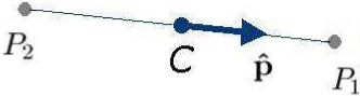
Figure 1: Pair of intersection points $P_{1},P_{2}$ with distance $2r$, midpoint $C$ and unit direction vector $\mathrm{\mathbf{\hat{p}}}$ of the connecting line segment.

2.4 Straight Lines

Using the same definitions the straight line through $P_{1}$ and $P_{2}$ is given by

$$P_{1}\wedge P_{2}\wedge\mathrm{\mathbf{n}}=2r\mathrm{\mathbf{\hat{p}}}\wedge C\wedge\mathrm{\mathbf{n}}=2r\{\mathrm{\mathbf{\hat{p}}}\wedge\mathrm{\mathbf{c}}\,\,\mathrm{\mathbf{n}}-\mathrm{\mathbf{\hat{p}}}N\}$$ (18)

2.5 Circles

$$P_{1}\wedge P_{2}\wedge P_{3}=\alpha\{\mathrm{\mathbf{c}}\wedge I_{c}+\frac{1}{2}[(c^{2}+r^{2})I_{c}-2\mathrm{\mathbf{c}}(\mathrm{\mathbf{c}}{\sf\hskip 8.61108pt\rule{0.6458pt}{6.45831pt}\rule{6.45831pt}{0.6458pt}\hskip 2.15277pt}I_{c})]\mathrm{\mathbf{n}}+I_{c}\mathrm{\mathbf{\bar{n}}}-(\mathrm{\mathbf{c}}{\sf\hskip 8.61108pt\rule{0.6458pt}{6.45831pt}\rule{6.45831pt}{0.6458pt}\hskip 2.15277pt}I_{c})N\}$$

$$=\alpha(C+\frac{1}{2}r^{2}\mathrm{\mathbf{n}})\wedge\{I_{c}+\mathrm{\mathbf{n}}(C{\sf\hskip 8.61108pt\rule{0.6458pt}{6.45831pt}\rule{6.45831pt}{0.6458pt}\hskip 2.15277pt}I_{c})\}$$ (19)

describes a circle through the three points $P_{1}$, $P_{2}$ and $P_{3}$ with center $\mathrm{\mathbf{c}}$, radius $r$, and circle plane bivector

$$I_{c}=\frac{(\mathrm{\mathbf{p}}_{1}-\mathrm{\mathbf{p}}_{2})\wedge(\mathrm{\mathbf{p}}_{2}-\mathrm{\mathbf{p}}_{3})}{\alpha}\enspace,$$ (20)

where the scalar $\alpha>0$ is chosen such that

$$I_{c}^{2}=-1\enspace.$$ (21)

For the inner product we use the left contraction        in (19) as discussed in section 2.1. For $\mathrm{\mathbf{c}}\wedge I_{c}=0$ (origin $\mathrm{\mathbf{\bar{n}}}$ in circle plane) and the conformal center (17) we get

$$P_{1}\wedge P_{2}\wedge P_{3}=-\alpha\{C-\frac{1}{2}r^{2}\mathrm{\mathbf{n}}\}I_{c}N.$$ (22)

2.6 Planes

Using the same $\alpha$, $C$ and $I_{c}$ as for the circle

$$P_{1}\wedge P_{2}\wedge P_{3}\wedge\mathrm{\mathbf{n}}=\alpha\,\,C\wedge I_{c}\wedge\mathrm{\mathbf{n}}=\alpha\{\mathrm{\mathbf{c}}\wedge I_{c}\mathrm{\mathbf{n}}-I_{c}N\}$$ (23)

defines a plane through $P_{1}$, $P_{2}$, $P_{3}$ and infinity. For $\mathrm{\mathbf{c}}\wedge I_{c}=0$ (origin $\mathrm{\mathbf{\bar{n}}}$ in plane) we get

$$P_{1}\wedge P_{2}\wedge P_{3}\wedge\mathrm{\mathbf{n}}=-\alpha I_{c}N.$$ (24)

2.7 Spheres

$$P_{1}\wedge P_{2}\wedge P_{3}\wedge P_{4}=\beta(C-\frac{1}{2}r^{2}\mathrm{\mathbf{n}})IN$$ (25)

defines a sphere through $P_{1}$, $P_{2}$, $P_{3}$ and $P_{4}$ with radius $r$, conformal center $C$, unit volume trivector $I=\mathrm{\mathbf{e}}_{1}\mathrm{\mathbf{e}}_{2}\mathrm{\mathbf{e}}_{3}$, and scalar

$$\beta=(\mathrm{\mathbf{p}}_{1}-\mathrm{\mathbf{p}}_{2})\wedge(\mathrm{\mathbf{p}}_{2}-\mathrm{\mathbf{p}}_{3})\wedge(\mathrm{\mathbf{p}}_{3}-\mathrm{\mathbf{p}}_{4})\,\,I^{-1}\enspace.$$ (26)

3 Full Meet of Two Circles in One Plane

The meet of two circles (comp. Fig. 2)

$$V_{1}=(C_{1}-\frac{1}{2}r_{1}^{2}\mathrm{\mathbf{n}})I_{c}N,\,\,\,\,\,\,V_{2}=(C_{2}-\frac{1}{2}r_{2}^{2}\mathrm{\mathbf{n}})I_{c}N\enspace,$$ (27)

with conformal centers $C_{1},C_{2}$, radii $r_{1},r_{2}$, in one plane $I_{c}$ (containing the origin $\mathrm{\mathbf{\bar{n}}}$), and join four-vector $J=I_{c}N$ is

$$M=(V_{1}{\sf\hskip 8.61108pt\rule{0.6458pt}{6.45831pt}\rule{6.45831pt}{0.6458pt}\hskip 2.15277pt}J^{-1}){\sf\hskip 8.61108pt\rule{0.6458pt}{6.45831pt}\rule{6.45831pt}{0.6458pt}\hskip 2.15277pt}V_{2}$$ (28)

$$=\frac{1}{2}[(\mathrm{\mathbf{c}}_{1}^{2}-r_{1}^{2})-(\mathrm{\mathbf{c}}_{2}^{2}-r_{2}^{2})]I_{c}+\frac{1}{2}[(\mathrm{\mathbf{c}}_{2}^{2}-r_{2}^{2})\mathrm{\mathbf{c}}_{1}-(\mathrm{\mathbf{c}}_{1}^{2}-r_{1}^{2})\mathrm{\mathbf{c}}_{2}]I_{c}\mathrm{\mathbf{n}}+(\mathrm{\mathbf{c}}_{2}-\mathrm{\mathbf{c}}_{1})I_{c}\mathrm{\mathbf{\bar{n}}}+\mathrm{\mathbf{c}}_{1}\wedge\mathrm{\mathbf{c}}_{2}I_{c}N$$ (29)

$$=\ldots=\frac{d}{2r}P_{1}\wedge P_{2}$$ (30)

with

$$d=\mid\mathrm{\mathbf{c}}_{2}-\mathrm{\mathbf{c}}_{1}\mid\enspace,$$ (31)

$$r^{2}=\frac{M^{2}}{(M\wedge\mathrm{\mathbf{n}})^{2}}=d^{2}\{\frac{r_{1}^{2}r_{2}^{2}}{d^{4}}-\frac{1}{4}(1-\frac{r_{1}^{2}}{d^{2}}-\frac{r_{2}^{2}}{d^{2}})^{2}\}$$ (32)

and [like in (14)]

$$\mathrm{\mathbf{p}}_{1}=\mathrm{\mathbf{c}}+r\mathrm{\mathbf{\hat{p}}},\,\,\,\mathrm{\mathbf{p}}_{2}=\mathrm{\mathbf{c}}-r\mathrm{\mathbf{\hat{p}}}\enspace,$$ (33)

$$\mathrm{\mathbf{c}}=\mathrm{\mathbf{c}}_{1}+\frac{1}{2}(1+\frac{r_{1}^{2}-r_{2}^{2}}{d^{2}})(\mathrm{\mathbf{c}}_{2}-\mathrm{\mathbf{c}}_{1}),\,\,\,\,\,\,\mathrm{\mathbf{\hat{p}}}=\frac{\mathrm{\mathbf{c}}_{2}-\mathrm{\mathbf{c}}_{1}}{d}I_{c}\enspace.$$ (34)

We further get independent of $r^{2}$

$$M\wedge\mathrm{\mathbf{n}}=d\mathrm{\mathbf{\hat{p}}}\wedge C\wedge\mathrm{\mathbf{n}}\enspace,$$ (35)

which is in general a straight line through $P_{1},P_{2}$, and in particular for $r^{2}=0$ $(M^{2}=0,\,\,\mathrm{\mathbf{p}}_{1}=\mathrm{\mathbf{p}}_{2}=\mathrm{\mathbf{c}})$ the tangent line at the intersection point. Note that $r^{2}$ may become negative (depending on $r_{1}$ and $r_{2}$, for details compare Fig. 4). The vector from the first circle center $\mathrm{\mathbf{c}}_{1}$ to the middle $\mathrm{\mathbf{c}}$ of the point pair is

$$\mathrm{\mathbf{c}}-\mathrm{\mathbf{c}}_{1}=\frac{1}{2}(1+\frac{r_{1}^{2}-r_{2}^{2}}{d^{2}})(\mathrm{\mathbf{c}}_{2}-\mathrm{\mathbf{c}}_{1})\enspace,$$ (36)

with (oriented) length

$$d_{1}=\frac{1}{2}(d+\frac{r_{1}^{2}-r_{2}^{2}}{d})$$ (37)

This length $d_{1}$, half the intersection point pair distance $r$ and the circle radius $r_{1}$ are related by

$$r^{2}+d_{1}^{2}=r_{1}^{2}\enspace.$$ (38)

We therefore observe (comp. Fig. 2, 3 and 4) that (38)

• describes for $r^{2}>0$ all points of real intersection (on the circle $V_{1}$) of the two circles.

• For $r^{2}<0$ (38) becomes the locus equation of the virtual points of intersection, i.e. two hyperbola branches that extend symmetrically on both sides of the circle $V_{1}$ (assuming e.g. that we move $V_{2}$ relative to $V_{1}$).

• The sequence of circle meets of Fig. 3 clearly illustrates, that as e.g. circle $V_{2}$ moves from the right side closer to circle $V_{1}$, also the virtual intersection points approach along the hyperbola branch $(r^{2}<0)$ on the same side of $V_{1}$, until the point of outer tangence $(d=r_{1}+r_{2},\,\,r=0)$. Then we have real intersection points $(r^{2}>0)$ until inner tangence occurs $(d=r_{2}-r_{1},\,\,r=0$). Reducing $d<r_{2}-r_{1}$ even further leads to virtual intersection points, wandering outwards on the same side hyperbola branch as before until $d$ becomes infinitely small. Moving $C_{2}$ over to the other side of $C_{1}$ repeats the phenomenon just described on the other branch of the hyperbola (symmetry to the vertical symmetry axis of the hyperbola through $C_{1}$).

• The transverse symmetry axis line of the two hyperbola branches is given by $C_{1}\wedge C_{2}\wedge\mathrm{\mathbf{n}}$, i.e. the straight line through the two circle centers.

• The assymptotics are at angles $\pm\frac{\pi}{4}$ to the symmetry axis.

• The radius $r_{1}$ is the semitransverse axis segment.

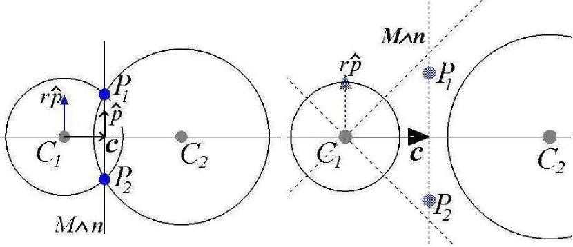
Figure 2: Two intersecting circles with centers $C_{1},C_{2}$, intersecting in points $P_{1},P_{2}$ at distance $2r$, with midpoint $\mathrm{\mathbf{c}}$ and unit direction vector $\mathrm{\mathbf{\hat{p}}}$ of the connecting line segment. Left side: Real intersection ($r_{2}<d<r_{1}+r_{2}$), right side: Virtual intersection ($d>r_{1}+r_{2}$).

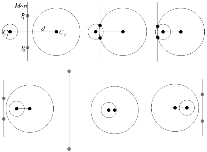
Figure 3: Real and virtual intersection points (33) and vertical carrier line $M\wedge\mathrm{\mathbf{n}}$ of (35) for two circles with radii $r_{1}<r_{2}$ and centers $C_{1},C_{2}$ at central distances $d$ (31). Top left: $d>r_{1}+r_{2},\,\,r^{2}<0$. Top center: $r_{2}<d<r_{2}+r_{1},\,\,r^{2}>0$. Top right: $r_{2}-r_{1}<d<r_{2},\,\,r^{2}>0$. Bottom left: $d+r_{1}<r_{2},\,\,r^{2}<0$. Bottom center: smaller $d$. Bottom right: similar to bottom left, but $C_{1}$ on other side of $C_{2}$.

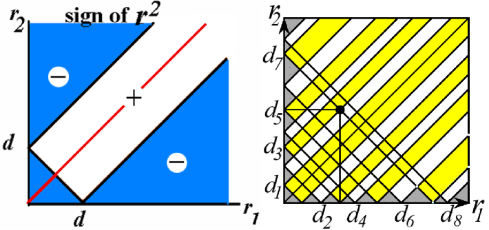
Figure 4: Left side: Positive (+) and negative ($-$) signs of $r^{2}$ depending on the radii of the two circles and the circle center distance $d$. $r=0$ (0) on the border lines (shape of an open U tilted in the $r_{1}=r_{2}$ direction), which separate ($-$) and (+) regions. Right side: Black dot for case $r_{1}<r_{2}$. Eight different values of $d$ are indicated, showing the tilted U-shaped (0) border lines between the ($-$) and (+) regions. $d_{1}<r_{2}-r_{1}$ ($-$), $d_{2}=r_{2}-r_{1}$ (0), $d_{3}=r_{1}$ (+), $r_{2}-r_{1}<d_{4}<r_{2}$ (+), $d_{5}=r_{2}$ (+), $r_{2}<d_{6}<r_{1}+r_{2}$ (+), $d_{7}=r_{1}+r_{2}$ (0) and $d_{8}>r_{1}+r_{2}$ ($-$).

4 Full Meet of Circle and Straight Line in One Plane

Now we turn our attention to the meet of a circle with center $C_{1}$, radius $r_{1}$ in plane $I_{c},\,\,I_{c}^{2}=-1$ (including the origin $\mathrm{\mathbf{\bar{n}}}$)

$$V_{1}=(C_{1}-\frac{1}{2}r_{1}^{2}\mathrm{\mathbf{n}})I_{c}N\enspace,$$ (39)

and a straight line through $C_{2}$, with direction $\mathrm{\mathbf{\hat{p}}}$ and in the same plane $I_{c}$,

$$V_{2}=\mathrm{\mathbf{\hat{p}}}\wedge C_{2}\wedge\mathrm{\mathbf{n}}=\mathrm{\mathbf{\hat{p}}}\wedge\mathrm{\mathbf{c}}_{2}\mathrm{\mathbf{n}}-\mathrm{\mathbf{\hat{p}}}N\enspace.$$ (40)

(For convenience $C_{2}$ be selected such that $d=\mid\mathrm{\mathbf{c}}_{2}-\mathrm{\mathbf{c}}_{1}\mid$ is the distance of the circle center $C_{1}$ from the line $V_{2}$. See Fig. 5.)

The meet of $V_{1}$ and $V_{2}$ is

$$M=(V_{1}{\sf\hskip 8.61108pt\rule{0.6458pt}{6.45831pt}\rule{6.45831pt}{0.6458pt}\hskip 2.15277pt}J^{-1}){\sf\hskip 8.61108pt\rule{0.6458pt}{6.45831pt}\rule{6.45831pt}{0.6458pt}\hskip 2.15277pt}V_{2}=\ldots=\frac{-1}{2r}P_{1}\wedge P_{2}$$ (41)

with the join $J=I_{c}N$,

$$r^{2}=M^{2}=r_{1}^{2}-d^{2}\enspace,$$ (42)

and

$$\mathrm{\mathbf{p}}_{1}=\mathrm{\mathbf{c}}_{2}+r\mathrm{\mathbf{\hat{p}}},\,\,\,\mathrm{\mathbf{p}}_{2}=\mathrm{\mathbf{c}}_{2}-r\mathrm{\mathbf{\hat{p}}}\enspace.$$ (43)

$r$ and $\mathrm{\mathbf{\hat{p}}}$ have the same meaning as in (14). Note that $r^{2}<0$ for $d>r_{1}$.

We observe that

• Equations (38) and (42) are remarkably similar.

• The point pair $P_{1}\wedge P_{2}$ is now always on the straight line $V_{2}$, and has center $C_{2}$!

• For $r^{2}>0$ $(d<r_{1})$

  $$r^{2}+d^{2}=r_{1}^{2}$$ (44)

  describes the real intersections of circle and straight line.

• For $r^{2}<0$ $(d>r_{1})$

  $$r^{2}+d^{2}=r_{1}^{2}$$ (45)

  describes the virtual intersections of circle and straight line.

• The general formula $M\wedge\mathrm{\mathbf{n}}=-V_{2}$ holds for all values of $r$, even if $r^{2}=M^{2}=0\,\,(\mathrm{\mathbf{p}}_{1}=\mathrm{\mathbf{p}}_{2}=\mathrm{\mathbf{c}}_{2})$. In this special case $V_{2}$ is tangent to the circle.

• In all other repects, the virtual intersection locus hyperbola has the same properties (symmetry, transverse symmetry axis, assymptotics and semitransverse axis segment) as that of the meet of two circles in one plane.

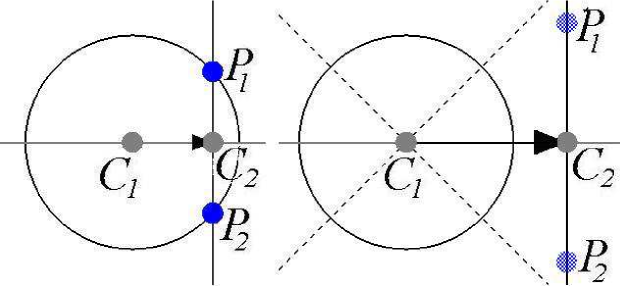
Figure 5: Real and virtual intersections of circle and straight line.

5 Full Meet of Two Spheres

Let us assume two spheres (see Fig. 6)

$$V_{1}=(C_{1}-\frac{1}{2}r_{1}^{2}\mathrm{\mathbf{n}})IN,\,\,\,\,\,\,V_{2}=(C_{2}-\frac{1}{2}r_{2}^{2}\mathrm{\mathbf{n}})IN\enspace.$$ (46)

with centers $C_{1},C_{2}$, radii $r_{1},r_{2}$, and (3+2)–dimensional pseudoscalar join $J=IN$. The meet of these two spheres is

$$M=(V_{1}{\sf\hskip 8.61108pt\rule{0.6458pt}{6.45831pt}\rule{6.45831pt}{0.6458pt}\hskip 2.15277pt}J^{-1}){\sf\hskip 8.61108pt\rule{0.6458pt}{6.45831pt}\rule{6.45831pt}{0.6458pt}\hskip 2.15277pt}V_{2}$$

$$=\frac{1}{2}[(\mathrm{\mathbf{c}}_{1}^{2}-r_{1}^{2})-(\mathrm{\mathbf{c}}_{2}^{2}-r_{2}^{2})]I-\frac{1}{2}[(\mathrm{\mathbf{c}}_{2}^{2}-r_{2}^{2})\mathrm{\mathbf{c}}_{1}-(\mathrm{\mathbf{c}}_{1}^{2}-r_{1}^{2})\mathrm{\mathbf{c}}_{2}]I\mathrm{\mathbf{n}}+(\mathrm{\mathbf{c}}_{1}-\mathrm{\mathbf{c}}_{2})I\mathrm{\mathbf{\bar{n}}}+\mathrm{\mathbf{c}}_{1}\wedge\mathrm{\mathbf{c}}_{2}IN$$

$$=\ldots=\,\,d(C+\frac{1}{2}r^{2}\mathrm{\mathbf{n}})\wedge\{I_{c}+\mathrm{\mathbf{n}}(C{\sf\hskip 8.61108pt\rule{0.6458pt}{6.45831pt}\rule{6.45831pt}{0.6458pt}\hskip 2.15277pt}I_{c})\}\enspace,$$ (47)

where $r$ and $d$ are defined as for the case of intersecting two circles [$r^{2}=-M^{2}/(M\wedge\mathrm{\mathbf{n}})^{2}$, note the sign!] We further introduced in (47) the plane bivector

$$I_{c}=\frac{(\mathrm{\mathbf{c}}_{1}-\mathrm{\mathbf{c}}_{2})}{d}I$$ (48)

and the vector (see Fig. 6)

$$\mathrm{\mathbf{c}}=\mathrm{\mathbf{c}}_{1}+\frac{1}{2}(1+\frac{r_{1}^{2}-r_{2}^{2}}{d^{2}})(\mathrm{\mathbf{c}}_{2}-\mathrm{\mathbf{c}}_{1})\enspace.$$ (49)

Comparing (19) and (47) we see that $M$ is a conformal circle multivector with radius $r$, oriented parallel to $I_{c}$ in the plane $M\wedge\mathrm{\mathbf{n}}=dC\wedge I_{c}\wedge\mathrm{\mathbf{n}}$, and with center $C$.

Regarding the formula

$$r^{2}+d_{1}^{2}=r_{1}^{2}$$ (50)

with $d_{1}=|\mathrm{\mathbf{c}}-\mathrm{\mathbf{c}}_{1}|$ it remains to observe that

• equation (50) describes for $r^{2}>0$ $(d_{1}<r_{1})$ the real radius $r$ circles of intersection of two spheres.

• These intersection circles are centered at $C=\mathrm{\mathbf{c}}+\frac{1}{2}c^{2}\mathrm{\mathbf{n}}+\mathrm{\mathbf{\bar{n}}}$ in the plane $M\wedge\mathrm{\mathbf{n}}$ perpendicular to the center connecting straight line $C_{1}\wedge C_{2}\wedge\mathrm{\mathbf{n}}$, i.e. parallel to the bivector of (48).

• For $r^{2}=0$, $M\wedge\mathrm{\mathbf{n}}$ gives still the (conformal) tangent plane trivector of the two spheres.

• We have for $r^{2}<0$ $(d_{1}>r_{1})$ virtual circles of intersection forming a hyperboloid with two sheets, as shown in Fig. 7.

• The transverse symmetry axis (straight) line of the two sheet hyperboloid is $C_{1}\wedge C_{2}\wedge\mathrm{\mathbf{n}}$.

• The discussion of the meet of two circles in section 3 related to Fig. 3 and Fig. 4 applies also to the case of the meet of two spheres. $r^{2}$ is now the squared radius of real and virtual meets (circles instead of point pairs).

• The asymptotic double cone has angle $\pi/4$ relative to the transverse symmetry axis.

• The sphere radius (e.g. $r_{1}$) is again the semitransverse axis segment of the two sheet hyperboloid (assuming e.g. that we move $V_{2}$ relative to $V_{1}$).

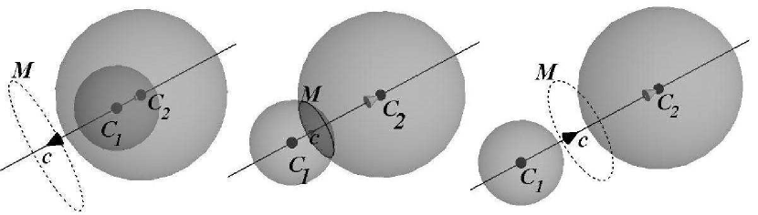
Figure 6: Real and virtual intersections of two spheres ($r_{1}<r_{2}$). Left: $d<r_{2}-r_{1}<r_{2}$, center: $r_{2}<d<r_{1}+r_{2}$, right: $d>r_{1}+r_{2}$.

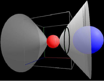
Figure 7: Two sheet hyperboloid of virtual intersections of two spheres.

6 Full Meet of Sphere and Plane

Let $V_{1}$ be a conformal sphere four-vector [as in (46)] and $V_{2}$ a conformal plane four-vector [(23) with normalization $\alpha=1$]. The analogy to the case of circle and straight line is now obvious. For the virtual $(r^{2}<0)$ intersections we get the same two sheet hyperboloid as for the case of sphere and sphere, but now both real and virtual intersection circles are always on the plane $V_{2}$, as shown in Fig. 8. The general formula $M\wedge\mathrm{\mathbf{n}}=V_{2}$ holds for all values of $r$, even if $r^{2}=M^{2}=0$. In this special case $V_{2}$ is tangent to the sphere.

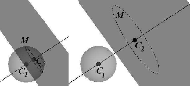
Figure 8: Real and virtual intersections of sphere and plane.

References

- [1] D. Hestenes, New Foundations for Classical Mechanics (2nd ed.), Kluwer, Dordrecht, 1999.
-
[2]
E.M.S. Hitzer,
Learning about Conic Sections with Geometric Algebra and Cinderella,
in E.M.S. Hitzer, R. Nagaoka, H. Ishi (eds.),
Proc. of Innovative Teaching of Mathematics with Geometric Algebra
Nov. 2003, Research Institute for Mathematical Sciences (RIMS),
Kyoto, Japan, RIMS 1378, pp. 89–104 (2004).
Interactive online presentation:
http://sinai.mech.fukui-u.ac.jp/ITM2003/presentations/Hitzer/page1.html - [3] H. Grassmann, A new branch of math., tr. by L. Kannenberg, Open Court, 1995. H. Grassmann, Extension Theory, tr. by L. Kannenberg, AMS, Hist. of Math., 2000.
-
[4]
C. Perwass,
Analysis of Local Image Structure using Intersections of Conics,
Technical Report, University of Kiel, (2004)
http://www.perwass.de/published/perwass_tr0403_v1.pdf - [5] L. Dorst, Interactively Exploring the Conformal Model, Lecture at Innovative Teaching of Mathematics with Geometric Algebra 2003, Nov. 20-22, Kyoto University, Japan. L. Dorst, D. Fontijne, An algebraic foundation for object-oriented Euclidean geometry, in E.M.S. Hitzer, R. Nagaoka, H. Ishi (eds.), Proc. of Innovative Teaching of Mathematics with Geometric Algebra Nov. 2003, Research Institute for Mathematical Sciences (RIMS), Kyoto, Japan, RIMS 1378, pp. 138–153 (2004).
- [6] L. Dorst, The Inner Products of Geometric Algebra, in L. Dorst et. al. (eds.), Applications of Geometric Algebra in Computer Science and Engineering, Birkhaeuser, Basel, 2002.
- [7] C. Doran, A. Lasenby, J. Lasenby, Conformal Geometry, Euclidean Space and Geometric Algebra, in J. Winkler (ed.), Uncertainty in Geometric Computations, Kluwer, 2002.
- [8] D. Hestenes, G. Sobczyk, Clifford Algebra to Geometric Calculus, Kluwer, Dordrecht, reprinted with corrections 1992.
- [9] G. Casanova, L’Algebre De Clifford Et Ses Applications, Special Issue of Adv. in App. Cliff. Alg. Vol 12 (S1), (2002).
- [10] P. Lounesto, Clifford Algebras and Spinors, 2nd ed., CUP, Cambridge, 2001.
-
[11]
G. Sobczyk,
Clifford Geometric Algebras in Multilinear Algebra and Non-Euclidean Geometries,
Lecture at Computational Noncommutative Algebra and Applications, July 6-19, 2003,
http://www.prometheus-inc.com/asi/algebra2003/abstracts/sobczyk.pdf - [12] D. Hestenes, H. Li, A. Rockwood, New Algebraic Tools for Classical Geometry, in G. Sommer (ed.), Geometric Computing with Clifford Algebras, Springer, Berlin, 2001.
- [13] E.M.S. Hitzer, KamiWaAi - Interactive 3D Sketching with Java based on Cl(4,1) Conformal Model of Euclidean Space, Advances in Applied Clifford Algebras 13(1), pp. 11-45 (2003).
- [14] E.M.S. Hitzer, G. Utama, The GeometricAlgebra Java Package – Novel Structure Implementation of 5D GeometricAlgebra for Object Oriented Euclidean Geometry, Space-Time Physics and Object Oriented Computer Algebra, to be published in Mem. Fac. Eng. Univ. Fukui, 53(1) (2005).
- [15] E.M.S. Hitzer, Euclidean Geometric Objects in the Clifford Geometric Algebra of {Origin, 3-Space, Infinity}, to be published in Bulletin of the Belgian Mathematical Society - Simon Stevin.
- [16] GAViewer homepage http://www.science.uva.nl/ga/viewer/index.html
- [17] Cinderella website, http://www.cinderella.de/
- [18] C. Perwass, CLUCalc website, http://www.clucalc.info/