Microlensing by a wide-separation planet: detectability and boundness

Abstract

The microlensing technique has proven sensitive to Earth-like and/or wide-separation extrasolar planets. The unbiased spatial distribution of extrasolar planets with respect to host stars is crucial in studying the planet formation processes. If one can characterize the planetary microlensing light curves whether they are produced by a wide-separation planet or a free-floating planet, it will greatly help to establish the spatial distribution of extrasolar planets without contamination by free-floating planets. Previous studies have shown that the effect of the host star on the microlensing by the accompanying wide-separation planet can be significant enough to be detected by the high-frequency microlensing experiments for typical microlensing parameters. Here, we further explore the detection condition of a wide-separation planet through the perturbation induced by the planetary caustic for various microlensing parameters, especially for the size of the source stars. By constructing the fractional deviation maps at various positions in the space of microlensing parameters, we find that the pattern of the fractional deviation depends on the ratio of the source radius to the caustic size, and the ratio satisfying the observational threshold varies with the star-planet separation. We have also obtained the upper limits of the source size that allows the detection of the signature of the host star as a function of the separation for given observational threshold. It is shown that this relation further leads one to a simple analytic condition for the star-planet separation to detect the boundness of wide-separation planets as a function of the mass ratio and the source radius. For example, when 5$\%$ of the detection threshold is assumed, for a source star with the radius of $\sim 1$ $R_{\odot}$, an Earth-mass planet and a Jupiter-mass planet can be recognized of its boundness when it is within the separation range of $\sim 10$ AU and $\sim 30$ AU, respectively. We also compare the separation ranges of detection by the planetary caustic with those by the central caustic. It is found that when the microlensing light curve caused by the planetary caustic happens to be analyzed, one may afford to support the boundness of the wide-separation planet farther than when that caused by the central caustic is analyzed. Finally, we conclude by briefly discussing the implication of our findings on the next-generation microlensing experiments.

1 INTRODUCTION

Up to the present, 19 extrasolar planets have been discovered towards the Galactic bulge by the microlensing experiments operating in the survey and follow-up mode (Bond et al., 2004; Udalski et al., 2005; Beaulieu et al., 2006; Gould et al., 2006; Gaudi et al., 2008; Bennett et al., 2008; Dong et al., 2009; Sumi et al., 2010; Janczak et al., 2010; Miyake et al., 2011; Batista et al., 2011; Muraki et al., 2011; Yee et al., 2012; Bennett et al., 2012; Bachelet et al., 2012; Han et al., 2013; Kains et al., 2013). A planetary microlensing event shows a perturbation, lasting for a short-duration of $t_{\rm E,p}\sim\sqrt{q}t_{\rm E}$, typically about a day and a few hours for the mass ratio $q$ corresponding to a Jupiter-mass planet and an Earth-mass planet, respectively, to the standard light curve induced by a lens star, whose typical timescale is the Einstein timescale for the lens system $t_{\rm E}$ (Mao & Paczynski, 1991; Gould & Loeb, 1992). Continuous monitoring with a high cadence is, therefore, prerequisite to avoid missing planetary microlensing events.

To monitor a wide field of view continuously with high cadence, existing microlensing experiments, such as, the OGLE collaboration and MOA collaboration, have recently changed the camera to expand the field of view or planned to upgrade the telescope. Next-generation surveys, with a wider field of view and higher cadence such as Korea Microlensing Telescope Network (KMTNet) and Wide-Field Infrared Survey Telescope (WFIRST) are being prepared to search the extrasolar planets by the microlensing technique in ground and space, respectively. The main aim of KMTNet project is to find sub-Earth-mass planets using three 1.6 m wide field (2 $\times$ 2 degrees field of view) optical telescopes located in Chile, South Africa, and Australia (Kim et al., 2010). The key goal of WFIRST mission is to discover planets down to 0.1 Earth-mass in the separation range wider than 0.5 AU, consequently to dispense a complete statistical census of the planet in our Galaxy (Bennett, 2011).

Such surveys with a frequent sampling can be sufficiently sensitive to wide-separation and free-floating planets, and thus enable us to detect wide-separation planets as well as free-floating planets which are otherwise very difficult to find by other planet search techniques, such as, radial velocity technique, transit technique, direct imaging, or pulsar timing analysis (Bennett & Rhie, 2002; Han & Kang, 2003; Sumi et al., 2011; Bennett et al., 2012). In fact, Sumi et al. (2011) recently reported the discovery of unbound or possibly distantly orbiting populations with a planetary-mass, based on microlensing survey observations on MOA-II phase between 2006 and 2007. According to their statistical estimates the number of such populations is approximately twice that of main-sequence stars in the Galaxy.

If one can tell via microlensing observations whether these planets are still bound to their host stars or freely floating without host stars, essential information can be provided on the spatial distribution of extrasolar planets with respect to host stars without contamination by unbound planets so that the core accretion theory can be tightly constrained (Laughlin, Bodenheimer, & Adams, 2004; Ida, & Lin, 2005; Kennedy, Kenyon, & Bromley, 2006; Kennedy & Kenyon, 2008). A free-floating planet itself is also important in constraining the planet formation processes since it is related to the processes, such as star-planet scattering (Holman & Wiegert, 1999; Musielak et al., 2005; Malmberg et al., 2011), planet-planet scattering (Rasio & Ford, 1996; Weidenschilling & Marzari, 1996; Lin & Ida, 1997; Ford & Rasio, 2008; Veras & Raymond, 2012), and star death (Veras et al., 2011).

Several suggestions have been made to distinguish wide-separation planets from free-floating planets (Di Stefano & Scalzo, 1999a, b; Han & Kang, 2003; Han et al., 2005; Han, 2009b; Di Stefano, 2012a, b). Basically, a planetary microlensing event can be inferred that it is caused by a wide-separation planet if the light curve shows any signature of the host star, such as, a long-term bump, blended light, or a signal of the planetary caustic in the light curve. The former two signatures depend on the source trajectory and lens flux, respectively, and need additional long-term observations for confirmation, while the last signature will become important in the next-generation surveys with high survey monitoring frequency. Han & Kang (2003) investigated the microlensing properties of wide-orbit planets and found that the signature of the central star can be detected for a large fraction of Jupiter mass planetary system for a typical source size and star-planet distance. Han et al. (2005) comprehensively discussed these three methods for the detection of a host star, and found that one-third of all events should show signatures of its host star regardless of the planet separation through these methods.

In this paper we investigate the condition in terms of lensing parameters, particularly, the size of source stars, under which signatures of the host star in the planetary microlensing light curve can be detected. We construct magnification maps for various source radii by the inverse ray-shooting method, taking the limb darkening into consideration, since the planetary caustic located close to the wide-separation planet is so small that the finite source effect becomes critical for a given photometric accuracy. As a result, we obtain a general empirical formula for the upper limit on the ratio of source size to the planetary caustic size that allows to detect the signature of the host star as a function of the separation, which asymptotically approaches to a constant as the separation goes to infinity, as approximated by Chang & Refsdal (1979, 1984). We also compare the separation ranges to detect the boundness of the planet to the host star through the channel of the central and planetary caustics.

This paper is organized as follows. We briefly describe properties of a planetary caustic for a wide-separation planetary system in §2. We discuss how we construct the fractional deviation maps in §3. We present conditions to detect signatures of a host star in the planetary microlensing light curve in §4. Finally, we summarize and conclude our results in §5.

2 PROPERTIES OF PLANETARY CAUSTIC

A planetary perturbation occurs when a source star crosses or passes by the caustic resulted from a star-planet system. Provided that an extrasolar planetary system has a single planet, the planetary system produces one, two or three disconnected caustics depending on the separation between a planet and its host star. In a wide-separation planetary system, in which the projected separation of the planet and the host star is larger than the upper limit of the lensing zone, two disconnected caustics are generated: central and planetary caustics. Here, the position of the planetary caustic is so close to the planet that sometimes the planetary caustic is located within the Einstein ring due to the planet.

The planetary caustic structure can be expressed by a analytic form (e.g., Witt & Mao, 1995; Bozza, 2000). The formulae of x$-$ and y$-$components of the caustics in the polar coordinate system, $x(\theta)$ and $y(\theta)$, are given by

$$x(\theta) = (s-\frac{m_{1}}{s})+(\varepsilon_{1}-\frac{m_{2}}{\varepsilon_{1}})\cos\theta+\frac{m_{1}\varepsilon_{1}\cos\theta}{s^{2}}$$

$$+ (1+\frac{m_{2}}{\varepsilon_{1}^{2}})\varepsilon_{2}\cos\theta+\frac{m_{1}}{s^{3}}(\varepsilon_{2}s\cos\theta-\varepsilon_{1}^{2}\cos 2\theta),$$

$$y(\theta) = (\varepsilon_{1}-\frac{m_{2}}{\varepsilon_{1}})\sin\theta-\frac{m_{1}\varepsilon_{1}\sin\theta}{s^{2}}$$

$$+ (1+\frac{m_{2}}{\varepsilon_{1}^{2}})\varepsilon_{2}\sin\theta-\frac{m_{1}}{s^{3}}(\varepsilon_{2}s\sin\theta-\varepsilon_{1}^{2}\sin 2\theta),$$

where $\varepsilon_{1}$ and $\varepsilon_{2}$ are given by

$$\varepsilon_{1}=\left(m_{2}\frac{m_{1}\cos 2\theta\pm\sqrt{s^{4}-m_{1}^{2}\sin^{2}2\theta}}{s^{2}-m_{1}/s^{2}}\right)^{1/2},$$ (3)

$$\varepsilon_{2}=-\frac{m_{1}\varepsilon_{1}^{4}(m_{1}\varepsilon_{1}^{2}\cos\theta+m_{2}s^{2}\cos 3\theta)}{m_{2}s^{3}(m_{1}\varepsilon_{1}^{2}\cos 2\theta+m_{2}s^{2})}.$$ (4)

Here, $m_{1}$ and $m_{2}$ are the masses of lens star and planet, respectively, and $s$ is the projected separation between them normalized by the Einstein ring radius.

Hence, the planetary caustic size along the planet-star axis is

$$\Delta x=|x(0)-x(\pi)|=\frac{2\sqrt{m_{2}}}{s}\frac{m_{1}(2s^{2}+m_{1}+1)}{\sqrt{(s^{4}-m_{1})(s^{2}+m_{1})}}\;.$$ (5)

If we choose $m_{1}=1$ and $m_{2}=q=m_{2}/m_{1}$ (also see Han, 2006), then Equation 5 becomes

$$\Delta x\simeq\frac{4\sqrt{q}}{s\sqrt{s^{2}-1}}\;.$$ (6)

As shown in Equation 6, the planetary caustic size $\Delta x$ is proportional to $\sqrt{q}$ and inversely to $s^{2}$ when $s\gg 1$. Thus, a low mass planet with wide separation has a fairly small perturbation region.

3 FRACTIONAL DEVIATION MAP

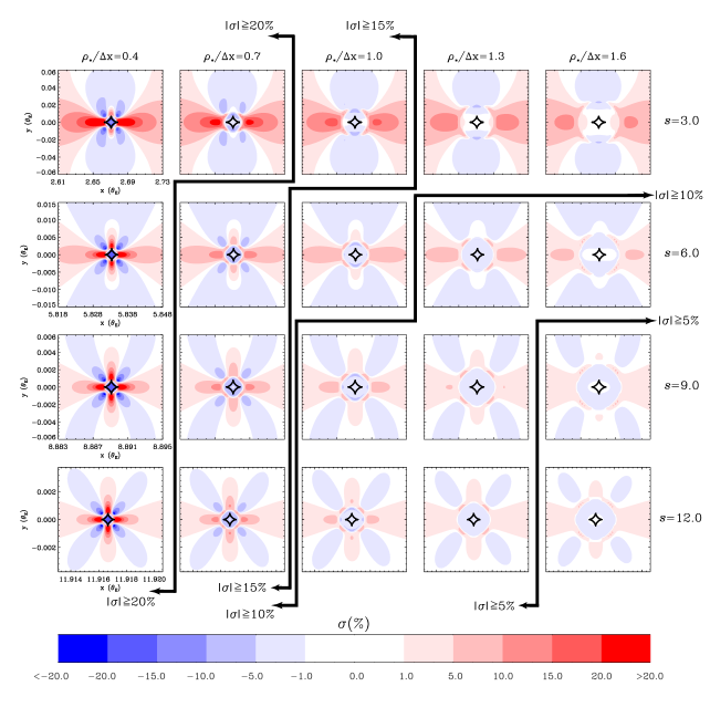
Figure 1: Maps of the fractional deviation in magnifications for various ratios of the source radius normalized by the planetary caustic size $\rho_{\star}/\Delta x$, where $\rho_{\star}=\theta_{\star}/\theta_{\rm E}$ and $\theta_{\star}$ being the angular radius of a source star, and normalized separation $s$ by the Einstein ring radius $\theta_{\rm E}$. The ratio of the source radius to the planetary caustic size $\rho_{\star}/\Delta x$ and the separation $s$ are marked on the top of each column and the right-hand side of each row, respectively. The panels are divided by thick black lines with arrows to outline in the parameter space the domains where regions with the amplitude of fractional deviations as indicated by the arrows can be found in the deviation maps. In each map, the contours are the levels of $\sigma=\pm 1\%$, $\pm 5\%$, $\pm 10\%$, $\pm 15\%$, and $\pm 20\%$, and the colors of blue and red tones are the regions with negative and positive $\sigma$, respectively, where lighter shades represent smaller $|\sigma|$ levels. We show $\sigma$ levels corresponding to each color in the scale-bar. The black curve at the center in each panel represents the caustic shape. In this particular plot, we set the Galactic distances of lens $D_{l}=6$ kpc and that of source star $D_{s}=8$ kpc. The lens star is located at the origin of coordination, i.e., ($x,y$)=(0,0).

In Figure 1, we show the fractional deviation map for various ratios of the source radius normalized by the planetary caustic size $\rho_{\star}/\Delta x$, where $\rho_{\star}=\theta_{\star}/\theta_{\rm E}$ and $\theta_{\star}$ being the angular radius of a source star, and normalized separation $s$ by the Einstein ring radius $\theta_{\rm E}$. The ratio of the normalized source radius and separation are denoted on the top of each column and on the right-hand side of each row, respectively.

The fractional deviation $\sigma$ is defined by

$$\sigma\equiv\frac{A-A_{\rm P}}{A_{\rm P}},$$ (7)

where the magnification of the planetary lensing $A$ results from a planet with its host star, and $A_{\rm P}$ from a planet alone, like the case of a free-floating planet. Note that $A_{\rm P}$ is scaled by the Einstein ring radius of the planet itself, $\theta_{\rm{E,P}}$, which is related to the Einstein ring radius for the total mass of the star-planet system, $\theta_{\rm E}$, as $\theta_{\rm{E,P}}=\theta_{\rm E}\sqrt{q/(1+q)}$. The position of the peak magnification of the planet itself, $\hat{s}$, is also adjusted to match the center of a planetary caustic of the star-planet system, i.e., $\hat{s}=s-1/s$.

Since a low mass planet with wide separation has a fairly small perturbation region, the finite source effect is crucial. We construct the magnification maps using the inverse ray-shooting method to include the finite source effect (Schneider & Weiss, 1986; Kayser et al., 1986; Wambsganss, 1997). In addition to the finite source effect, we also take into account the limb darkening effect by the surface of source star. On the surface of the source star, the specific intensity $I$ with the flux $F$ and the limb darkening coefficient of $\Gamma$ is given by

$$I=\frac{F}{\pi\theta_{\star}^{2}}[1-\Gamma(1-1.5\cos\phi)],$$ (8)

where $\phi$ is the angle between the normal direction to the star’s surface and the direction toward the observer (Milne, 1921; An et al., 2002). In this particular study, we adopt a fixed value of $\Gamma$ for all source stars, i.e., $\Gamma=0.5$. We also assume that the lens system with the mass ratio of $1\times 10^{-3}$ is located at $D_{l}=6$ kpc and the source star is at $D_{s}=8$ kpc.

The panels in Figure 1 are divided by thick black lines with arrows to outline in the parameter space the domains where regions with the amplitude of fractional deviations as indicated by the arrows can be found in the deviation maps. Note that the contours are drawn at the levels of $\sigma=\pm 1\%$, $\pm 5\%$, $\pm 10\%$, $\pm 15\%$, and $\pm 20\%$ as shown in the scale-bar. As one may expect, the fractional deviation decreases as the ratio of the source radius to the planetary caustic size and/or the projected separation increases.

4 LENSING BY A WIDE-SEPARATION PLANET

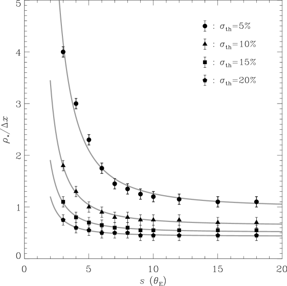
Figure 2: Upper limits on the ratio of the source radius to the planetary caustic size for $\sigma_{\rm{th}}=$ 5$\%$, 10$\%$, 15$\%$, and 20$\%$. The filled circles, triangles, squares, and pentagons represent the maximum values of $\rho_{\star}/\Delta{x}$ as a function of $s$ for different thresholds $\sigma_{\rm{th}}$, that is, $\sigma_{\rm{th}}=$ 5$\%$, 10$\%$, 15$\%$, and 20$\%$, respectively. The error bars mean the uncertainty on the determination of the upper limit of $\rho_{\star}/\Delta x$. The black curve is the fitting function, that is, Equation 9. See text for detailed discussions of this plot.

In Figure 2, we show the upper limits of normalized source radius $\rho_{\star}/\Delta x$ that allow to detect the signature of the host star as a function of the separation when a threshold $\sigma_{\rm{th}}$ is given. Different symbols represent different threshold $\sigma_{\rm{th}}$, that is, $\sigma_{\rm{th}}=$ 5$\%$, 10$\%$, 15$\%$, and 20$\%$ for filled circles, triangles, squares, and pentagons, respectively. The error bars mean the uncertainty on the determination of the upper limit of $\rho_{\star}/\Delta x$. When $s$ becomes much larger than unity, the magnification pattern can be approximated by the Chang & Refsdal (1979, 1984) lensing, and thus $\rho_{\star}/\Delta x$ is nearly constant independent of $s$. However, the planetary caustic becomes asymmetric and the size of the planetary caustic also becomes bigger as $s$ approaches unity. This is why $\rho_{\star}/\Delta x$ rapidly increases as $s$ gets close to unity since the major perturbation regions around the cusps of the planetary caustic are located outside of the Einstein ring size of planet mass.

Another point to note is that this upper limit on the source-caustic size ratio can be approximated by a fitting function,

$$\frac{\rho_{\star}}{\Delta x}(s)=\frac{C_{1}}{s\sqrt{s^{2}-1}}+C_{2}\;\;\textrm{for}\;s\geq 3,$$ (9)

with $C_{1}\simeq 0.3/\sigma_{\rm{th}}\sqrt{\sigma_{\rm{th}}}$ and $C_{2}\simeq 0.21/\sqrt{\sigma_{\rm{th}}}$, respectively, which is represented by solid curves. What we have seen here has interesting implications. For instance, this plot can be read to see how the finite source effect constrain the range of the projected separation when the detection threshold is given. In other words, one may obtain for a given source radius and a planet-star mass ratio the upper limit of the star-planet separation that allows the detection of caustic structure due to a host star. Specifically speaking, combining Equations 6 and 9, one obtains

$$s\leq\left(\frac{1+\sqrt{1+4R^{-2}}}{2}\right)^{1/2},$$ (10)

where

$$R\equiv\frac{-C_{2}+\sqrt{C_{2}^{2}+C_{1}\rho_{\star}/q^{1/2}}}{2C_{1}}.$$ (11)

In Figure 3, we show the upper limit of the star-planet separation to detect the boundness of the wide-separation planet as a function of the source radius and the mass of the planet (left panel), assuming for $\sigma_{\rm{th}}=5\%$, and of the detection threshold of fractional deviation and the mass of the planet (right panel), assuming for $R_{\star}=1\;R_{\odot}$. Dotted contours and gray scales represent the upper limit of the separation in units of AU. The planet mass $M_{\rm{p}}$ is given in a log scale in units of the solar mass $M_{\odot}$, the source radius $R_{\star}$ in the left panel is in units of the solar radius $R_{\odot}$. In this specific example, we set $D_{l}=6$ kpc, $D_{s}=8$ kpc, and the lens mass of 0.5 $M_{\odot}$.

According to the left panel, the maximum separation one can tell whether a planetary microlensing feature is caused by a bound planet becomes larger as the radius of the source star becomes smaller and/or the planet mass larger. In other words, as the source star is large and the finite source effect becomes important, one can only detect the existence of its host star when the planet is massive and planet-star separation is small. When 5$\%$ of the detection threshold is assumed, for a source star with the radius of $\sim 1$ $R_{\odot}$, an Earth-mass planet ($\log M_{\rm{p}}=-5.5$ $M_{\odot}$) and a Jupiter-mass planet ($\log M_{\rm{p}}=-3.0$ $M_{\odot}$) can be recognized of its boundness when it is within the separation range of $\sim 10$ AU and $\sim 30$ AU, respectively. Similarly, according to the right panel, the upper limit of the separation becomes larger as the detection threshold becomes lower. The photometric precision of KMTNet project is expected to meet $1\%$ at 21 magnitude in V band on 10 minute monitoring frequency and that of WFIRST mission is $\leq 1\%$ at 20.5 magnitude in J band on $\leq 15$ minute sampling cadence. Therefore, we expect that the next-generation microlensing experiments with high survey monitoring frequency and accurate photometry will discover wide-separation planets with various separations as analyzed in this study.

In Figure 4, we compare the separation ranges to detect the boundness of the wide-separation planet through the channel of the central and planetary caustics. The black curves represent the upper limits of the separation range induced by the planetary caustic for various source radii $R_{\star}=$ $1\;R_{\odot}$, $3\;R_{\odot}$, $5\;R_{\odot}$, and $7\;R_{\odot}$, while the gray curves represent by the central caustic that we calculate following Han (2009a). Results are given both in units of AU and $\theta_{\rm{E}}$. We take the same values of parameters as in Figure 3 for the distances of lens and source, and the lens mass, and assuming 5$\%$ of the detection threshold. The separation range to detect the boundness of the wide-separation planet induced by the planetary caustic is wider than that induced by the central caustic. What it means is that, when the microlensing light curve induced by the planetary caustic happens to be analyzed, one may afford to detect the boundness of the wide-separation planet farther than when that caused by the central caustic is analyzed.

5 CONCLUSION

The unbiased spatial distribution of extrasolar planets with respect to host stars is crucial in studying the planet formation processes. Massive and/or close extrasolar planets are likely to be detected by a commonly employed method. On the other hand, the microlensing technique can be sensitive to Earth-like and/or wide-separation planets. To obtain the spatial distribution of extrasolar planets without contaminating by free-floating planets, it is important to characterize the planetary microlensing light curves whether they are caused by a wide-separation planet or a free-floating planet.

Here, we analyze the condition in terms of lensing parameters, including the size of source stars, under which signatures of the host star in the planetary microlensing light curve can be detected. By constructing the fractional deviation maps at various positions in the space of microlensing parameters, we have obtained the upper limits of $\rho_{\star}/\Delta x$ that allow to detect the signature of the host star as a function of the separation when a threshold is given. We confirm that when $s\gg 1$ the Chang & Refsdal (1979, 1984) lensing well-approximate what we have found. We also note that a simple analytical function can be fit, as given in Equation 9. This relation further leads one to a simple analytic condition for the star-planet separation to detect the boundness of wide-separation planets as a function of the mass ratio and source radius, as shown in Figure 3. Finally, we have compared the separation ranges to detect the boundness of the wide-separation planet through the channel of the central and planetary caustics. As a result, we conclude that when the microlensing light curve caused by the planetary caustic happens to be analyzed, one may afford to support the boundness of the wide-separation planet farther than when that caused by the central caustic is analyzed. Therefore, we conclude that the next-generation microlensing experiments with high survey monitoring frequency are expected to add the number of wide-separation planets through the channel of the planetary caustic.

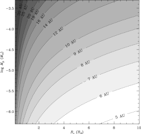
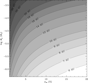
Figure 3: Upper limit of the star-planet separation to detect the boundness of the wide-separation planet as a function of the source radius and the mass of the planet (left panel), assuming for $\sigma_{\rm{th}}=5\%$, and as a function of the detection threshold of fractional deviation and the mass of the planet (right panel), assuming for $R_{\star}=1\;R_{\odot}$. Dotted contours and gray scales represent the upper limit of the separation in units of AU. The employed parameters in this example are $D_{l}=6$ kpc, $D_{s}=8$ kpc, and lens mass of 0.5 $M_{\odot}$.

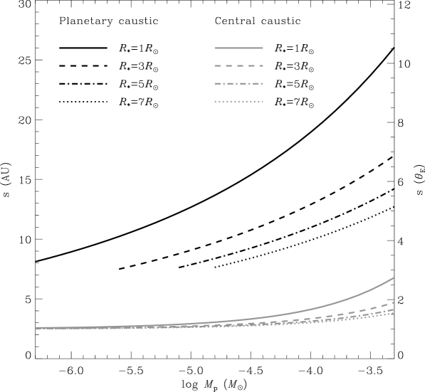
Figure 4: Comparison of the separation ranges to detect the boundness of the wide-separation planet through the channel of the central caustics with the planetary caustics. The upper limits of the separation ranges are plotted with the black and gray curves for the planetary and central caustics, respectively. We assume that the the distances of lens and source and the lens mass are $D_{l}=6$ kpc, $D_{s}=8$ kpc, and 0.5 $M_{\odot}$, and the detection threshold is 5$\%$.

References

- An et al. (2002) An J. H., et al., 2002, ApJ, 572, 521
- Bachelet et al. (2012) Bachelet E., et al., 2012, ApJ, 754, 73
- Batista et al. (2011) Batista, V., et al., 2011, A&A, 529, A102
- Bennett (2011) Bennett D. P., 2011, AAS, 43, #318.01
- Bennett & Rhie (2002) Bennett, D. P., & Rhie, S. H., 2002, ApJ, 574, 985
- Bennett et al. (2012) Bennett D. P., et al., 2012, ApJ, 757, 119
- Bennett et al. (2008) Bennett, D. P., et al., 2008, ApJ, 684, 663
- Beaulieu et al. (2006) Beaulieu, J.-P., et al., 2006, Nature, 439, 437
- Bond et al. (2004) Bond, I. A., et al., 2004, ApJL, 606, L155
- Bozza (2000) Bozza, V., 2000, A&A, 355, 423
- Chang & Refsdal (1984) Chang K., Refsdal S., 1984, A&A, 132, 168
- Chang & Refsdal (1979) Chang K., Refsdal S., 1979, Natur, 282, 561
- Di Stefano (2012a) Di Stefano, R., 2012a, ApJS, 201, 20
- Di Stefano (2012b) Di Stefano, R., 2012b, ApJS, 201, 21
- Di Stefano & Scalzo (1999a) Di Stefano, R., & Scalzo, R. A., 1999a, ApJ, 512, 564
- Di Stefano & Scalzo (1999b) Di Stefano, R., & Scalzo, R. A., 1999b, ApJ, 512, 579
- Dong et al. (2009) Dong, S., et al., 2009, ApJ, 698, 1826
- Ford & Rasio (2008) Ford, E. B., & Rasio, F. A., 2008, ApJ, 686, 621
- Gaudi et al. (2008) Gaudi, B. S., et al., 2008, Science, 319, 927
- Gould & Loeb (1992) Gould, A., & Loeb, A., 1992, ApJ, 396, 104
- Gould et al. (2006) Gould, A., et al., 2006, ApJL, 644, L37
- Han (2006) Han, C., 2006, ApJ, 638, 1080
- Han (2009a) Han, C., 2009a, ApJ, 691, 452
- Han (2009b) Han, C., 2009b, ApJ, 700, 945
- Han & Kang (2003) Han, C., & Kang, Y. W., 2003, ApJ, 596, 1320
- Han et al. (2013) Han C., et al., 2013, ApJ, 762, L28
- Han et al. (2005) Han C., et al., 2005, ApJ, 618, 962
- Holman & Wiegert (1999) Holman, M. J., & Wiegert, P. A., 1999, AJ, 117, 621
- Ida, & Lin (2005) Ida, S., & Lin, D. N. C., 2005, ApJ, 626, 1045
- Janczak et al. (2010) Janczak, J., et al., 2010, ApJ, 711, 731
- Kains et al. (2013) Kains N., et al., 2013, A&A, 552, A70
- Kayser et al. (1986) Kayser, R., Refsdal, S., & Stabell, R., 1986, A&A, 166, 36
- Kennedy & Kenyon (2008) Kennedy, G. M., & Kenyon, S. J., 2008, ApJ, 673, 502
- Kennedy, Kenyon, & Bromley (2006) Kennedy, G. M., Kenyon, S. J., & Bromley, B. C., 2006, ApJ, 650, L139
- Kim et al. (2010) Kim S.-L., et al., 2010, SPIE, 7733
- Laughlin, Bodenheimer, & Adams (2004) Laughlin, G., Bodenheimer, P., & Adams, F. C., 2004, ApJ, 612, L73
- Lin & Ida (1997) Lin, D. N. C., & Ida, S., 1997, ApJ, 477, 781
- Malmberg et al. (2011) Malmberg, D., Davies, M. B., & Heggie, D. C., 2011, MNRAS, 411, 859
- Mao & Paczynski (1991) Mao, S., & Paczynski, B., 1991, ApJL, 374, L37
- Milne (1921) Milne, E. A., 1921, MNRAS, 81, 361
- Miyake et al. (2011) Miyake N., et al., 2011, ApJ, 728, 120
- Muraki et al. (2011) Muraki Y., et al., 2011, ApJ, 741, 22
- Musielak et al. (2005) Musielak, Z. E., Cuntz, M., Marshall, E. A., & Stuit, T. D., 2005, A&A, 434, 355
- Rasio & Ford (1996) Rasio, F. A., & Ford, E. B., 1996, Science, 274, 954
- Schneider & Weiss (1986) Schneider, P., & Weiss, A., 1986, A&A, 164, 237
- Sumi et al. (2011) Sumi, T., et al., 2011, Nature, 473, 349
- Sumi et al. (2010) Sumi, T., et al., 2010, ApJ, 710, 1641
- Udalski et al. (2005) Udalski, A., et al., 2005, ApJL, 628, L109
- Veras & Raymond (2012) Veras, D., & Raymond, S. N., 2012, MNRAS, 421, L117
- Veras et al. (2011) Veras, D., Wyatt, M. C., Mustill, A. J., Bonsor, A., & Eldridge, J. J., 2011, MNRAS, 417, 2104
- Wambsganss (1997) Wambsganss, J., 1997, MNRAS, 284, 172
- Weidenschilling & Marzari (1996) Weidenschilling, S. J., & Marzari, F., 1996, Nature, 384, 619
- Witt & Mao (1995) Witt, H. J., & Mao, S., 1995, ApJL, 447, L105
- Yee et al. (2012) Yee J. C., et al., 2012, ApJ, 755, 102