Analytic results in the position-dependent mass Schrodinger problem

Abstract

We investigate the Schrodinger equation for a particle with a nonuniform solitonic mass density. First, we discuss in extent the (nontrivial) position-dependent mass $V(x)=0$ case whose solutions are hypergeometric functions in $\tanh^{2}x$. Then, we consider an external hyperbolic-tangent potential. We show that the effective quantum mechanical problem is given by a Heun class equation and find analytically an eigenbasis for the space of solutions. We also compute the eigenstates for a potential of the form $V(x)=V_{0}\sinh^{2}x$.

I Introduction

The study of the Schrodinger equation with a position-dependent mass (PDM) has been a matter of interest since the early days of Solid State physics. Indeed, many of the important questions in the theory of solids concern the non-relativistic motion of electrons in periodic lattices perturbed by the effect of impurities, as it happens in typical semiconductors slater .

The theoretical understanding of transport phenomena in semiconductors of a position-dependent chemical composition is at the root of this problem. The PDM idea arises after the effect of the periodic field on the electrons. In this context, the electron mass was originally replaced by a mass tensor whose elements were determined by the unperturbed band structure luttingerkohn . To be more specific, the electronic wave packet near the top or the bottom of an energy band is the quantum mechanical entity related to the effective PDM concept. As explained by von Roos vonroos , the Wannier-Slater theorem slater ; wannier in its simplest form states that the envelope function $F(r,t)$ (for the conduction band, for instance) obeys a Schrodinger-like equation $[E(k)(-i\nabla)+V(r)]F(r,t)=i\hbar\dot{F}(r,t)$ where $E(k)$ represents the conduction band energy of the unperturbed crystal, $k$ is the crystal momentum and $V(r)$ is the potential due to external sources (e.g. electromagnetic fields) or superficial impurities. In simple cases, by starting with the one-electron approximation of the many-body Hamiltonian one can approximate this equation with a position-dependent effective mass Schrodinger equation for the envelope

$$\left[-\frac{\hbar^{2}}{2m(r)}\nabla^{2}+E(0)+V(r)\right]F(r,t)=i\hbar\dot{F}(r,t).$$ (1)

In nonuniform semiconductors, with a position-dependent chemical composition, extensions of the theorem require not only modifications of the potential term but also of the kinetic operator. In fact, it is already evident in Eq. (1) where the kinetic term is manifestly non-hermitian. A natural improvement to fix this problem is the use of a symmetrized operator gora ; bastard

$$\hat{T}=\frac{1}{4}\left(\frac{1}{m(r)}\hat{p}^{2}+\hat{p}^{2}\frac{1}{m(r)}\right)$$ (2)

but neither this solves completely the question shewell so several other orderings were postulated in subsequent years vonroos ; BDD ; tdlee ; zhukroemer ; likhun ; thomsenetc ; young ; einevol1 ; einevol2 ; levyleblon .

In the last decade, the present subject has gained renewed interest for both mathematical and phenomenological reasons. Issues such as hermiticity, operator ordering and solubility together with application and uses of the PDM Schrodinger equation related to molecular and atomic physics willatzenlassen2007 ; chinos200407 ; severtazcan2008 ; quesne2008 ; mustafa2009 ; midyaroy2009 ; ardasever2011 ; hamdouni2011 ; mustafa2011 ; midya2011 ; sinha2011 ; sinha2012 as well as to supersymmetry and relativistic problems plastino99 ; alhaidari2004 ; tanaka2006 ; mustafa2008 ; midyaetal have been matter of intense activity in the fields of quantum mechanics and condensed matter physics in the last years. In the present paper, after a clarifying discussion of the ordering problem (Sec. II), we analyze the PDM Hamiltonian for a solitonic mass profile (Sec. III). First, we study in detail the nontrivial PDM $V=0$ case (Sec. IV) and thereafter add a $\tanh x$ potential function (Sec. VI). This potential is related to nanowire step structures with a varying radius willatzenlassen2007 and hyperbolic versions of Scarf scarf , Rosen-Morse rosenmorse and Manning-Rosen potentials manningrosen of interest in modeling molecular vibrations and intermolecular forces, recently discussed in e.g. znojil ; ozlem ; souzadutra ; chinos2008 ; chinos2009 ; chinos201011 ; correa2012 ; bharali2013 ; canadian2013 . In Sec. V we also discuss a special case of the form $\sinh^{2}x$. In all these cases we analytically find the complete set of solutions to the PDM Schrodinger equations by means of a series of coordinate transformations and wave function mappings. In Sec. VII we draw our conclusions.

II The PDM ordering problem

We start this paper by analyzing the Hermitian kinetic operator

$$\hat{T}=\,\frac{1}{8}\left\{\left(m^{-1}(\vec{r})\,\hat{p}^{2}\,+\,\,\hat{p}^{2}\,m^{-1}(\vec{r})\right)+\,m^{\alpha}(\vec{r})\,\hat{p}\ m^{\beta}(\vec{r})\,\hat{p}\ m^{\gamma}(\vec{r})\,\,+\,m^{\gamma}(\vec{r})\,\hat{p}\ m^{\beta}(\vec{r})\,\hat{p}\ m^{\alpha}(\vec{r})\,\right\}$$ (3)

with the following constraint on the parameters $\alpha+\beta+\gamma=-1$ as proposed in vonroos . The first term, not considered originally, is here added just in order to include the usual symmetrized or Weyl ordered operator tdlee (viz. $\alpha\,=\,\gamma=\,0$) in the general expression.

In one dimension, when one properly commutes the momentum operators $\hat{p}=-i\hbar\frac{d}{dx}$ to the right, the following effective operator is obtained

$$\hat{T}\,=\,\frac{1}{2\,m}\,\hat{p}^{2}\,+\,\frac{i\hbar}{2}\frac{dm/dx}{m^{2}}\,\,\hat{p}\,\,+\,U_{\rm k}\left(x\right),$$ (4)

where

$$U_{\rm k}\left(x\right)=\frac{-\hbar^{2}}{4m^{3}}\left[\left(\alpha+\gamma-1\right)\frac{m}{2}\frac{d^{2}m}{dx^{2}}+\left(1-\alpha\gamma-\alpha-\gamma\right)\left(\frac{dm}{dx}\right)^{2}\right]$$ (5)

As a result of the general proposal (3), we obtain an effective potential $U_{\rm k}$ of kinematic origin, which is a different function for different combinations of the mass power parameters $\alpha,\beta,\gamma$. This lack of uniqueness can be eliminated by imposing the condition

$$\alpha\,+\,\gamma\,=\,1\,=\alpha\,\gamma\,+\,\alpha\,+\,\gamma$$ (6)

which implies that for $\alpha=0$ and $\gamma=1$, or $\alpha=1$ and $\gamma=0$, the kinetic operator $\hat{T}$ is free of the uncertainties coming from the commutation rules of Quantum Mechanics ($[\hat{x},\hat{p}]=i\hbar$). Note that condition (6) excludes the possibility of a Weyl ordering (and consequently the kinetic operator used in likhun ; see DA ).

Even in this case, although free of the ambiguous kinematic potential (5), the effective Schrödinger equation will contain a first order derivative term. For an arbitrary external potential $V(x)$ the non-ambiguous PDM Schrödinger equation results

$$\left[\frac{1}{2m}\,\hat{p}^{2}+\frac{i\hbar}{2}\frac{m^{\prime}}{m^{2}}\,\hat{p}+V(x)\right]\Psi(x)=E\Psi(x).$$ (7)

III Smooth mass profile

As we have seen, in order to avoid ambiguities from the beginning we were led to equation (7). It coincides with the Ben Daniel-Duke ordering of the PDM problem BDD . This ordering has recently been shown to be appropriate for the understanding of growth-intended geometrical nanostructures suffering from size variations, impurities, dislocations, and geometry imperfections willatzenlassen2007 , and is also consistent with the analysis made in renan where the Dirac equation was considered.

After substitution of the momentum operator, Eq. (7) can be written as

$$\left\{\frac{d^{2}}{dx^{2}}-\frac{1}{m(x)}\frac{dm(x)}{dx}\frac{d}{dx}+\frac{2m(x)}{\hbar^{2}}[E-V(x)]\right\}\psi(x)=0.$$ (8)

Here we adopt the following smooth effective mass distribution

$$m(x)=m_{0}\textsf{sech}^{2}(ax)$$ (9)

because it is an appropriate representative of a solitonic profile (see e.g. iran and bagchi ) found in several effective models of condensed matter and low energy nuclear physics. In Eq. (9), $a$ is a scale parameter that widens the shape of the effective mass as it gets smaller. This is equivalent to diminish the mass and energy scales (see Eq. (10) ). In this case, the effective differential equation reads

$$\psi^{\prime\prime}(x)+2\tanh(x)\psi^{\prime}(x)+\frac{2m_{0}}{a^{2}\hbar^{2}}(E-V(x))\textsf{sech}^{2}(x)\psi(x)=0,$$ (10)

where we shifted $ax\rightarrow x$. By means of

$$\psi(x)=\cosh^{\nu}\!(x)\,\varphi(x)$$ (11)

it becomes

$$\varphi^{\prime\prime}(x)+2(\nu+1)\tanh(x)\varphi^{\prime}(x)+\left[\nu(\nu+2)\tanh^{2}\!x+(\nu+\frac{2m_{0}}{a^{2}\hbar^{2}}(E-V(x)))\textsf{sech}^{2}(x)\right]\varphi(x)=0$$ (12)

We next transform $x\rightarrow z$ by

$$\frac{dz}{dx}=\textsf{sech}\,x,$$ (13)

namely

$$\cos\,z=\textsf{sech}\,x,$$ (14)

which maps $(-\infty,\infty)\rightarrow(-\frac{\pi}{2},\frac{\pi}{2})$.

Now the equation in the $z$ variable reads

$$\varphi^{\prime\prime}(z)+(2\nu+1)\tan(z)\varphi^{\prime}(z)+\left[\nu+\nu(\nu+2)\tan^{2}(z)+\frac{2m_{0}}{a^{2}\hbar^{2}}(E-V(z))\right]\varphi(z)=0$$ (15)

If we choose $\nu=-1/2$ we can eliminate the first derivative, resulting in

$$-\frac{d^{2}\varphi(z)}{dz^{2}}+\left[\frac{1}{2}+\frac{3}{4}\tan^{2}(z)+\tilde{V}(z)\right]\varphi(z)=\mathcal{E}\varphi(z)$$ (16)

where $\tilde{V}(z)=\frac{2m_{0}}{a^{2}\hbar^{2}}V(z)$ and $\mathcal{E}=\frac{2m_{0}}{a^{2}\hbar^{2}}E$. This equation allows symmetric and antisymmetric solutions provided $\tilde{V}(z)$ (and correspondingly $V(x)$) is even.

We can see that Eq. (8) is thus equivalent to a regular constant-mass stationary Schrodinger equation, Eq.(16), for a particle of mass $m_{0}$ in a confining potential

$$\mathcal{V}(z)=\frac{1}{2}+\frac{3}{4}\tan^{2}(z)+\tilde{V}(z).$$ (17)

Its dynamics is restricted to within $z=(-\frac{\pi}{2},\frac{\pi}{2})$ where $\varphi(z=\pm\frac{\pi}{2})=0$.

IV The case $V(x)=0$

In the $V(x)=0$ case (see Fig. 1) we can analytically solve the Schrodinger equation (16) in terms of a new variable, $y=\cos z$, where $0<y<1$. Since $E>0$, we can define $k^{2}=2m_{0}E/(a^{2}\hbar^{2})$ and obtain

Figure 1: Potential in $z$ space; $V(x)=0$ or $\mathcal{V}(z)=\frac{1}{2}+\frac{3}{4}\tan^{2}(z)$.

$$\varphi^{\prime\prime}(y)+\frac{y}{y^{2}-1}\varphi^{\prime}(y)+\left(\frac{{}^{1}\!/{}_{\!2}-k^{2}}{y^{2}-1}-\frac{{}^{3}\!/{}_{\!4}}{y^{2}}\right)\varphi(y)=0.$$ (18)

Now, we define another wave function $\varphi(y)=y^{-1/2}h_{1}(y)$ in order to put it in a more familiar form

$$h_{1}^{\prime\prime}(y)+\left(\frac{-1}{y}+\frac{{}^{1}\!/{}_{\!2}}{y-1}+\frac{{}^{1}\!/{}_{\!2}}{y+1}\right)h_{1}^{\prime}(y)+\frac{-k^{2}y}{y(y-1)(y+1)}h_{1}(y)=0\,\,$$ (19)

This equation belongs to the second order fuchsian class hille and can be recognized as a special case of the Heun equation ronveaux

$$H^{\prime\prime}(y)+\left(\frac{\gamma}{y}+\frac{\delta}{y-1}+\frac{\varepsilon}{y-d}\right)H^{\prime}(y)+\frac{\alpha\beta y-q}{y(y-1)(y-d)}H(y)=0\,\,$$ (20)

where the parameters obey the fuchsian relation $\alpha+\beta+1=\gamma+\delta+\varepsilon$. In the neighborhood of each singularity two linearly independent local solutions can be identified by their characteristic exponents (two for each solution) out from the Frobenius series. Although not so well known as its relative, the hypergeometric Gauss equation, a set of 192 different expressions have been recently given for the Heun equation by means of a set of transformations of a group of automorphysms maier .

Since we want the solution to Eq.(8) about $x=0$ here we will look for solutions around the singularity $y=1$ where the characteristic exponents are $0$ and $1-\delta$. Therefore, the two L.I. local solutions of interest to Eq.20 are

$$H=H\big{(}1-d,-q+\alpha\beta,\alpha,\beta,\delta,\gamma;1-y\big{)}\hskip 142.26378pt$$ (21)

$$H=(1-y)^{1-\delta}\,H\big{[}1-d,-q+(\delta-1)\gamma d+(\alpha-\delta+1)(\beta-\delta+1),\,\beta-\delta+1,\alpha-\delta+1,2-\delta,\gamma;1-y\big{]}$$ (22)

IV.1 Even solutions

By comparing Eq.(19) and Eq.(20) and using the fuchsian relation above we identify $d=-1$, $q=0$, $\alpha=-{}^{1}\!/{}_{\!2}+{}^{1}\!/{}_{\!2}\sqrt{1+4k^{2}}$, $\beta=-{}^{1}\!/{}_{\!2}-{}^{1}\!/{}_{\!2}\sqrt{1+4k^{2}}$, $\gamma=-1$, $\delta={}^{1}\!/{}_{\!2}$ and $\varepsilon={}^{1}\!/{}_{\!2}$ resulting in

$$h_{1}^{(1)}(y)=H\left(2,-k^{2},\frac{-1+\sqrt{1+4k^{2}}}{2},\frac{-1-\sqrt{1+4k^{2}}}{2},{}^{1}\!/{}_{\!2},-1;1-y\right)\leavevmode\nobreak\ \leavevmode\nobreak\ \leavevmode\nobreak\ \leavevmode\nobreak\$$ (23)

$$h_{1}^{(2)}(y)=(1\!-\!y)^{1/2}\!H\!\left(\!2,-\frac{3+4k^{2}}{4},-\frac{\sqrt{1+4k^{2}}}{2},\frac{\sqrt{1+4k^{2}}}{2},{}^{3}\!/{}_{\!2},\!-1;1\!-\!y\right)\leavevmode\nobreak\ \leavevmode\nobreak\$$ (24)

for the first of the two L.I. solutions. Recalling that $y=\cos z$ we have

$$\varphi^{(1,2)}(z)=\sqrt{\sec z}\,h_{1}^{(1,2)}(\cos z)$$ (25)

for the potential $\mathcal{V}(z)$ [Eq. (17)] about $z=0$ . Finally, in the original $x$ space, the even solutions of the PDM differential equation for the quantum particle of mass $m(x)$ [Eq. (9)] read

$$\psi^{(1,2)}(x)=h_{1}^{(1,2)}(\textsf{sech}x).$$ (26)

Naturally, we still need to impose the relevant boundary conditions. This is easily done in $z$ since the potential diverges to $+\infty$ in $z=\pm\frac{\pi}{2}$ which implies $\varphi(z=\pm\frac{\pi}{2})=0$. The first solution is convergent only for $k^{2}=n(n+1)$ with $n=1,3,...$, and the second solution is not acceptable because it is not differentiable at $z=0$ (see below).

IV.2 Odd solutions

In order to obtain the odd solutions we first transform

$$\varphi(z)=\sin z\,\phi(z)$$ (27)

in Eq. (16), resulting in equation

$$\phi^{\prime\prime}(z)+2\cot z\,\phi^{\prime}(z)-\left(\frac{3}{2}+\frac{3}{4}\tan^{2}z\right)\phi(z)=-k^{2}\phi(z).$$ (28)

Now using again $y=\cos z$ we get

$$\phi^{\prime\prime}(y)+\frac{3y}{y^{2}-1}\phi^{\prime}(y)+\left(\frac{{}^{3}\!/{}_{\!2}-k^{2}}{y^{2}-1}-\frac{{}^{3}\!/{}_{\!4}}{y^{2}}\right)\phi(y)=0$$ (29)

and once more $\phi(y)=y^{-1/2}h_{2}(y)$ leads to

$$h_{2}^{\prime\prime}(y)+\left(\frac{-1}{y}+\frac{{}^{3}\!/{}_{\!2}}{y-1}+\frac{{}^{3}\!/{}_{\!2}}{y+1}\right)h_{2}^{\prime}(y)+\frac{-k^{2}y}{y(y-1)(y+1)}h_{2}(y)=0\,\,$$ (30)

As before $h_{2}(y)$ are local Heun functions around $y=1$ (namely $z=0$ and $x=0$)) given by

$$h_{2}^{(1)}(y)=H\left(2,-k^{2},\frac{1+\sqrt{1+4k^{2}}}{2},\frac{1-\sqrt{1+4k^{2}}}{2},\frac{3}{2},-1;1-y\right)\leavevmode\nobreak\ \leavevmode\nobreak\ \leavevmode\nobreak\ \leavevmode\nobreak\ \leavevmode\nobreak\$$ (31)

$$h_{2}^{(2)}(y)=(1\!-\!y)^{-1/2}H\!\left(\!2,{}^{1}\!/{}_{\!4}-k^{2},-\frac{\sqrt{1+4k^{2}}}{2},\frac{\sqrt{1+4k^{2}}}{2},\frac{1}{2},-1;1-y\right)\leavevmode\nobreak\ \leavevmode\nobreak\ \leavevmode\nobreak\$$ (32)

with the following identification of parameters $\alpha_{2}=\frac{1+\sqrt{1+4k^{2}}}{2}$, $\beta_{2}=\frac{1-\sqrt{1+4k^{2}}}{2}$, $\gamma_{2}=-1$ and $\delta_{2}=\varepsilon_{2}=\frac{3}{2}$. These solutions, in $z$ and $x$ space respectively, read

$$\varphi^{(1,2)}(z)\!\! = \!\!\sin\!z(\sec z)^{1/2}\leavevmode\nobreak\ h_{2}^{(1,2)}(\cos z)$$ (33)

$$\psi^{(1,2)}(x)\!\! = \!\!b\tanh x\leavevmode\nobreak\ h_{2}^{(1,2)}(\textsf{{sech}}x)\leavevmode\nobreak\ \leavevmode\nobreak\ \leavevmode\nobreak\ \leavevmode\nobreak\ \leavevmode\nobreak\$$ (34)

Here, the first solutions, $\varphi^{(1)}(z)$ and $\psi^{(1)}(x)$, converge only for $k^{2}=n(n+1)$, with $n>0$ even. Again, $\varphi^{(2)}(z)$ ($\psi^{(2)}(x)$) is not differentiable at the origin and we discard it.

IV.3 Hypergeometric solutions

In several cases, the Heun equation can be reduced to a ordinary hypergeometric equation. This is actually the present case, where we can see that the solutions are products of trigonometric functions and hypergeometric ones.

Indeed, Maier maier2005 has recently determined that for a nontrivial Heun equation ($\alpha\beta\neq 0$ or $q\neq 0$) its local solution $H(d,q,\alpha,\beta,\gamma,\delta;t)$ can be reduced to ${}_{2}F_{1}(a,b,c;R(t))$ where $a,b,c$ depend on $d,q,\alpha,\beta,\gamma$ and $R(t)$ is a polynomials of up to sixth order provided $q=\alpha\beta p$, where $(d,p)$ is one among a set of 23 different values.

In particular, the case ($d,p$)=($2,1$) allows a transformation $H(t)\rightarrow{}_{2}F_{1}(R(t))$ with $R(t)$ of order 2 or 4. Now the even and odd physically acceptable solutions [Eqs. (23) and (31)] can be written as

$$h_{\rm phys}^{(1)}(t)=H\left(2,\alpha_{1}\beta_{1},\alpha_{1},\beta_{1},\gamma_{1}^{\prime},\delta_{1}^{\prime};t\right)$$ (35)

$$h_{\rm phys}^{(2)}(t)=H\left(2,\alpha_{2}\beta_{2},\alpha_{2},\beta_{2},\gamma_{2}^{\prime},\delta_{2}^{\prime};t\right)$$ (36)

where $\alpha_{1,2}$ and $\beta_{1,2}$ are those defined in the previous section and $\gamma_{1}^{\prime}=1/2$, $\delta_{1}^{\prime}=-1$, $\gamma_{2}^{\prime}={}^{3}\!/{}_{\!2}$, $\delta_{2}^{\prime}=-1$ and $t=1-y$.

The equations above are Heun solutions corresponding to $(d,p)=(2,1)$ with redefined parameters. Thus, we can simply reduce them to hypergeometric expressions

$$h_{\rm phys}^{(1)}(t)=H\left(2,\alpha_{1}\beta_{1},\alpha_{1},\beta_{1},\gamma_{1}^{\prime},\delta_{1}^{\prime};t\right)=\!{}_{2}F_{1}\left(\frac{\alpha_{1}}{2},\frac{\beta_{1}}{2},\gamma_{1}^{\prime};t(2-t)\right)$$ (37)

$$h_{\rm phys}^{(2)}(t)=H\left(2,\alpha_{2}\beta_{2},\alpha_{2},\beta_{2},\gamma_{2}^{\prime},\delta_{2}^{\prime};t\right)=\!{}_{2}F_{1}\left(\frac{\alpha_{2}}{2},\frac{\beta_{2}}{2},\gamma_{2}^{\prime};t(2-t)\right)$$ (38)

Then, in terms of the space variables $z$ and $x$ the following

$$\varphi_{\rm phys}^{(1)}(z)=\sec^{\!1/2}\!z\ {}_{2}F_{1}\left(\frac{-1+\sqrt{1+4k^{2}}}{4},\frac{-1-\sqrt{1+4k^{2}}}{4},\frac{1}{2}\leavevmode\nobreak\ ;\,\sin^{2}\!z\right)$$ (39)

$$\varphi_{\rm phys}^{(2)}(z)=\sin\!z\sec^{\!1/2}\!z\ {}_{2}F_{1}\left(\frac{1+\sqrt{1+4k^{2}}}{4},\frac{1-\sqrt{1+4k^{2}}}{4},\frac{3}{2}\,;\,\sin^{2}\!z\right)$$ (40)

and

$$\psi_{\rm phys}^{(1)}(x)={}_{2}F_{1}\!\left(\frac{-1+\sqrt{1+4k^{2}}}{4},\frac{-1-\sqrt{1+4k^{2}}}{4},\frac{1}{2};\,\tanh^{2}\!x\right)\leavevmode\nobreak\ \leavevmode\nobreak\ \leavevmode\nobreak\ \leavevmode\nobreak\$$ (41)

$$\psi_{\rm phys}^{(2)}(x)=\tanh\!x\ {}_{2}F_{1}\!\left(\frac{1+\sqrt{1+4k^{2}}}{4},\frac{1-\sqrt{1+4k^{2}}}{4},\frac{3}{2};\tanh^{2}\!x\right)\,\,$$ (42)

are, respectively, the physically acceptable solutions to the equation.

It can be shown that $\psi_{\rm phys}^{(1,2)}$ are mutually orthogonal

$$\langle\psi_{n}^{(i)},\psi_{m}^{(j)}\rangle=\delta_{nm}\delta_{ij},$$ (43)

and generate a complete set of solutions to the problem. Here $i,j=1,2$ and $n,m$ represent the order of the solution.

IV.4 Conditions of existence

In Eq. (39), since $\lim_{(z\rightarrow\pm\frac{\pi}{2})}\ \sec\!z=\infty$, we must impose

$$\lim_{z\rightarrow\pm\frac{\pi}{2}}{}_{2}F_{1}\left(\frac{-1+\sqrt{1+4k^{2}}}{4},\frac{-1-\sqrt{1+4k^{2}}}{4},\frac{1}{2}\leavevmode\nobreak\ ;\,\sin(z)^{2}\right)=0.$$ (44)

Since, for this expression

$$\lim_{z\rightarrow\pm\frac{\pi}{2}}{}_{2}F_{1}\left(z\right)\rightarrow\frac{\sqrt{\pi}}{\Gamma\left(\frac{3}{4}-\frac{1}{4}\sqrt{1+4k^{2}}\right)\Gamma\left(\frac{3}{4}+\frac{1}{4}\sqrt{1+4k^{2}}\right)}$$ (45)

the vanishing condition results

$$\frac{3}{4}-\frac{1}{4}\sqrt{1+4k^{2}}=-p,\leavevmode\nobreak\ \leavevmode\nobreak\ p=0,1,...$$ (46)

for $k$ finite. Regrouping, we obtain

$$k^{2}=(2p+1)^{2}+(2p+1).$$ (47)

On the same token, for the antisymmetric solutions, Eq.(40), we need

$$\lim_{z\rightarrow\pm\frac{\pi}{2}}{}_{2}F_{1}\left(\frac{1+\sqrt{1+4k^{2}}}{4},\frac{1-\sqrt{1+4k^{2}}}{4},\frac{3}{2}\leavevmode\nobreak\ ;\,\sin^{2}\!z\right)=0.$$ (48)

Since, in this case,

$$\lim_{z\rightarrow\pm\frac{\pi}{2}}{}_{2}F_{1}\left(z\right)\rightarrow\frac{2\sqrt{\pi}}{k^{2}\Gamma\left(\frac{1}{4}-\frac{1}{4}\sqrt{1+4k^{2}}\right)\Gamma\left(\frac{1}{4}+\frac{1}{4}\sqrt{1+4k^{2}}\right)}$$ (49)

we need

$$\frac{1}{4}-\frac{1}{4}\sqrt{1+4k^{2}}=-q,\leavevmode\nobreak\ \leavevmode\nobreak\ q=0,1,...$$ (50)

which, after regrouping may be written as

$$k^{2}=2q(2q+1).$$ (51)

Substituting $2p+1$ (2q) by $n$ in Eq. (47) (Eq. 51), the existence condition is in both cases $k^{2}=n(n+1)$, with $n$ odd (even) for even (odd) solutions, respectively.

Note that this result determines that energy is quantized as

$$E=\frac{a^{2}\hbar}{2m_{0}}\leavevmode\nobreak\ n(n+1),$$ (52)

with $n>0$, since energy cannot be zero.

The final expressions for symmetric and antisymmetric solutions (in $z$ and $x$ spaces) are thus

$$\varphi_{\rm phys}^{(1)}(z)\!\! = \!\!\sec^{\!1/2}\!z\ {}_{2}F_{1}\left(\frac{n}{2},-\frac{n+1}{2},\frac{1}{2}\leavevmode\nobreak\ ;\,\sin^{2}\!z\right)$$ (53)

$$\varphi_{\rm phys}^{(2)}(z)\!\! = \!\!\sin\!z\sec^{\!1/2}\!z\ {}_{2}F_{1}\left(\frac{n+1}{2},-\frac{n}{2},\frac{3}{2}\,;\,\sin^{2}\!z\right)$$ (54)

and

$$\psi_{\rm phys}^{(1)}(x)\!\! = \!\!{}_{2}F_{1}\!\left(\frac{n}{2},-\frac{n+1}{2},\frac{1}{2}\leavevmode\nobreak\ ;\,\tanh^{2}\!x\right)\leavevmode\nobreak\ \leavevmode\nobreak\ \leavevmode\nobreak\ \leavevmode\nobreak\$$ (55)

$$\psi_{\rm phys}^{(2)}(x)\!\! = \!\!\tanh\!x\ {}_{2}F_{1}\!\left(\frac{n+1}{2},-\frac{n}{2},\frac{3}{2}\,;\,\tanh^{2}\!x\right).$$ (56)

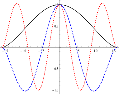
Figure 2: Symmetric solutions in $z$ space, Eq. (53), for $n=1$ (solid line), $n=3$ (dashed line) and $n=5$ (dotted line).

Figure 3: Symmetric normalized solutions in $x$ space , Eq. (55) (with $a$=1), for $n=1$ (solid line), $n=3$ (dashed line) and $n=5$ (dotted line).

We illustrate Eqs. (53) to (56) in Figs. 2, 3, 4 and 5.

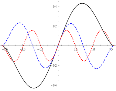
Figure 4: Antisymmetric solutions in $z$ space, Eq. (54), for $n=2$ (solid line), $n=4$ (dashed line) and $n=6$ (dotted line).

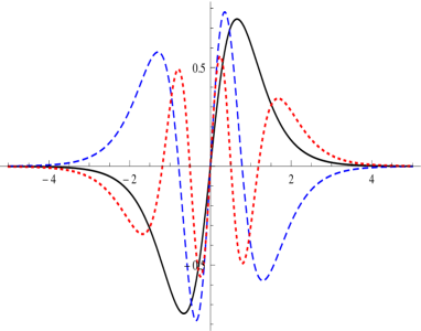
Figure 5: Antisymmetric normalized solutions in $x$ space, Eq. (56) (with $a$=1), for $n=2$ (solid line), $n=4$ (dashed line) and $n=6$ (dotted line).

In $x$ space we can get physical information about the position dependent mass particle. Figs. 3 and 5 show the increasing probability space density of the states around the origin.

V A special $V(x)=\sinh^{2}x$ case

It is interesting to note that in $z$ space, the confining problem defined by Eq. (16) becomes trivial for the potential $V(z)=-{3a^{2}\hbar^{2}}\tan^{2}z/{8m_{0}}+$cons. This corresponds to a $x$ space potential function

$$V(x)=-\frac{3a^{2}\hbar^{2}}{8m_{0}}\sinh^{2}x\,+\rm cons.$$ (57)

in Eq. (10).

Although this sets a nontrivial differential equation, the related full effective potential $\cal V$(z), Eq. (17), is just constant and therefore the exact solutions to the PDM problem can be easily obtained. Interestingly, this would be a much more difficult task in the constant-mass case.

The two L.I. solutions in $z$ space read

$$\varphi^{(1)}(z)\!\! = \!\!\sqrt{\frac{2}{\pi}}\cos\left((2n+1)\,z\right]$$ (58)

$$\varphi(z)\!\! = \!\!\sqrt{\frac{2}{\pi}}\sin\left(2n\,z\right)$$ (59)

where we have chosen cons.=$-a^{2}\hbar^{2}/4m_{0}$ in Eq. (57). Making them vanish at the border $z=\pm\pi/2$ quantizes the energy by

$$\mathcal{E}=\frac{a^{2}\hbar^{2}\pi^{2}}{8m_{0}}n^{2}$$ (60)

where $n\in\mathbb{N}$. Recalling Eq. (11), in $x$ space we obtain

$$\psi^{(1)}(x)\!\! = \!\!C_{1}\sqrt{\frac{2}{\pi}}\textsf{sech}^{1/2}\!x\,\textsf{sech}\big{[}(2n+1)\,x\big{]}$$ (61)

$$\psi^{(2)}(x)\!\! = \!\!C_{2}\sqrt{\frac{2}{\pi}}\textsf{sech}^{1/2}\!x\,\tanh(2n\,x),$$ (62)

see Fig. 6.

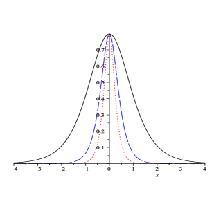
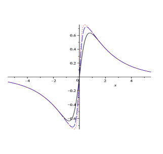
Figure 6: (a) Symmetric solutions [Eq.(61)] and (b) antisymmetric solutions [Eq. (62)] for $n=1$ (solid black line), $n=2$ (dashed blue line), and $n=3$ (dotted red line).

VI The tanh(x) case

In order to solve the associated differential equation we return to Eq. (16). According to Eq. (14) in the PDM problem the potential $V(x)=V_{0}\tanh\!x$ corresponds to $\tilde{V}(z)=\mathcal{V}_{0}\sin(z)$, where $\mathcal{V}_{0}=2m_{0}V_{0}/(a^{2}\hbar^{2})$. Now, the analysis of section IV implies that the PDM Schrödinger equation can be transformed into

$$-\frac{d^{2}\varphi(z)}{dz^{2}}+\mathcal{V}(z)\varphi(z)=\mathcal{E}\varphi(z)$$ (63)

with

$$\mathcal{V}(z)=\frac{1}{2}+\frac{3}{4}\tan^{2}(z)+\mathcal{V}_{0}\sin(z),$$ (64)

See Fig. 7. By means of the ansatz

$$\varphi(z)=\sqrt{\sec z}\ h(z)$$ (65)

the equation above can be written as

$$h^{\prime\prime}(z)+\tan\!z\,h^{\prime}(z)+(\mathcal{E}-\mathcal{V}_{0}\sin\!z)\,h(z)=0.$$ (66)

Figure 7: The effective potential $\mathcal{V}(z)$, Eq. (64), when $V(x)=V_{0}\tanh\!x$, for $\mathcal{V}_{0}=3$ (solid blue line), $\mathcal{V}_{0}=1$ (dashed gold line), $\mathcal{V}_{0}=-1$ (dash-dotted green line) and $\mathcal{V}_{0}=-3$ (dotted red line).

With a transformation of coordinates given by

$$y={}^{1}\!/{}_{\!2}+{}^{1}\!/{}_{\!2}\sin\!z,$$ (67)

we obtain

$$h^{\prime\prime}(y)+\left[\frac{-(\mathcal{V}_{0}+\mathcal{E})+2\mathcal{V}_{0}y}{y(y-1)}\right]h(y)=0.$$ (68)

Equation (68) is thus a particular case of the confluent Heun equation ronveaux ; hounkonnou ; fiziev

$$Hc^{\prime\prime}(y)\!+\!\left(\alpha\!+\!\frac{\beta+1}{y}+\frac{\gamma+1}{y-1}\right)Hc^{\prime}(y)\!+\!\left[\left(\delta+\frac{\alpha}{2}(\beta+\gamma+2)\right)y\!+\!\eta+\frac{\beta}{2}+\frac{1}{2}(\gamma\!-\!\alpha)(\beta+1)\right]\frac{1}{y(y-1)}Hc(y)=0\leavevmode\nobreak\ \leavevmode\nobreak\$$ (69)

By identifying $\alpha=0,\,\,\beta=\gamma=-1,\,\,\delta=2\mathcal{V}_{0},\,\,\eta={}^{1}\!/{}_{\!2}-\mathcal{V}_{0}-\mathcal{E},$ the local solutions of Eq. (68) about $y=0$ are given by

$$h^{(1)}(y)\!\! = \!\!y^{-\beta}Hc(\alpha,-\beta,\gamma,\delta,\eta;y)$$ (70)

$$h^{(2)}(y)\!\! = \!\!Hc^{\dagger}(\alpha,\beta,\gamma,\delta,\eta;y),$$ (71)

where $Hc^{\dagger}(y)$ is the second independent solution, so-called concomitant confluent Heun function used when $\beta=-1$ fizievCQG . Since this solution diverges logarithmically when $y\rightarrow 0$ the only physically acceptable solutions are thus

$$\varphi(z)=\frac{{}^{1}\!/{}_{\!2}+{}^{1}\!/{}_{\!2}\sin(z)}{\sqrt{\cos(z)}}\,Hc(0,1,-1,2\mathcal{V}_{0},{}^{1}\!/{}_{\!2}-\mathcal{V}_{0}-\mathcal{E};{}^{1}\!/{}_{\!2}+{}^{1}\!/{}_{\!2}\sin{z})\,\,$$ (72)

with $\varphi(z\rightarrow\pm\pi/2)=0$ for the allowed $\mathcal{E}$ and $\mathcal{V}_{0}$ as imposed by the boundary conditions. Parity is not a defined symmetry in this expression for any eigenvalue. However, as we see in Fig. 8 and Fig. 9 some eigenfunctions are (a) quasi-symmetric while others are (b) quasi-antisymmetric. Note that they alternate each other, as expected. In the original variable $x$ (recall eqs. (14) and (11)) these solutions, which we plot in Fig. 9, read

$$\psi(x)=\left({{}^{1}\!/{}_{\!2}+{}^{1}\!/{}_{\!2}\tanh{x}}\right)\,Hc(0,1,-1,2\mathcal{V}_{0},{}^{1}\!/{}_{\!2}-\mathcal{V}_{0}-\mathcal{E};{}^{1}\!/{}_{\!2}+{}^{1}\!/{}_{\!2}\tanh{x})\,\,$$ (73)

The energy eigenvalues can be numerically computed by imposing appropriate boundary conditions, namely, $\psi(x\rightarrow+\infty)=0$, ie. $\psi(y=1)=0$, with $y={}^{1}\!/{}_{\!2}+{}^{1}\!/{}_{\!2}\tanh\!x.$ A Frobenius expansion for Eq. (73) about $y=0$

$$\psi(y)=\sum_{n=0}^{\infty}c_{n}y^{n}$$ (74)

allows this calculation. For simplicity we choose $\mathcal{V}_{0}=1$ for which we obtain the list of eigenvalues presented in Table 1 (for $n$ up to 25).

Table 1: Energy eigenvalues of the Schrodinger equation for potential (64).

$\leavevmode\nobreak\ \leavevmode\nobreak\ \leavevmode\nobreak\ \leavevmode\nobreak\ \mathcal{E}_{1}$	$\leavevmode\nobreak\ \leavevmode\nobreak\ \leavevmode\nobreak\ \leavevmode\nobreak\ \mathcal{E}_{2}$	$\leavevmode\nobreak\ \leavevmode\nobreak\ \leavevmode\nobreak\ \leavevmode\nobreak\ \mathcal{E}_{3}$	$\leavevmode\nobreak\ \leavevmode\nobreak\ \leavevmode\nobreak\ \leavevmode\nobreak\ \mathcal{E}_{4}$	$\leavevmode\nobreak\ \leavevmode\nobreak\ \leavevmode\nobreak\ \leavevmode\nobreak\ \mathcal{E}_{5}$	$\leavevmode\nobreak\ \leavevmode\nobreak\ \leavevmode\nobreak\ \leavevmode\nobreak\ \mathcal{E}_{6}$
$1.9503339$	$6.0115779$	$12.0083261$	$20.0055193$	$30.0038467$	$42.0028139$

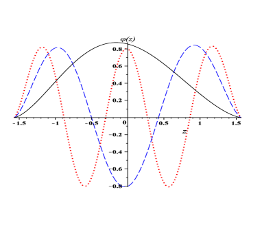
Figure 8: Normalized solutions, Eq. (72) with $\mathcal{V}_{0}=1$, for (a) $\mathcal{E}_{1}$ (solid black line), $\mathcal{E}_{3}$ (dashed blue line), and $\mathcal{E}_{5}$ (dotted red line), and (b) $\mathcal{E}_{2}$ (solid black line), $\mathcal{E}_{4}$ (dashed blue line) and $\mathcal{E}_{6}$ (dotted red line).

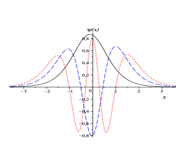
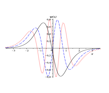
Figure 9: Normalized solutions, Eq. (73) with $\mathcal{V}_{0}=1$, for (a) $\mathcal{E}_{1}$ (solid black line), $\mathcal{E}_{3}$ (dashed blue line), and $\mathcal{E}_{5}$ (dotted red line), and (b) $\mathcal{E}_{2}$ (solid black line), $\mathcal{E}_{4}$ (dashed blue line) and $\mathcal{E}_{6}$ (dotted red line).

VII Conclusion

In this paper we have analyzed the Schrodinger equation for a nonuniform massive particle with a solitonic mass distribution. We have found the space of solutions related to a PDM Hermitian Hamiltonian defined by a non-ambiguous kinetic operator and an external potential. We have shown that while a special $\sinh^{2}x$ potential is easily worked out in this particular context the $V(x)=0$ case can be much more involved. The PDM $\tanh x$ potential case can be transformed into a Heun equation which we solved exactly by means of an analytic procedure. This potential is related to hyperbolic potentials of special interest for modeling atomic and molecular physics. Interestingly enough, for a long time absent in the literature, Heun functions have recently been found in very different contexts, see e.g. christiansencunha2011 ; christiansencunha2012 ; rumania ; bulgaria ; cvetic2011 ; herzog . Besides exactly obtaining all the solutions in the three cases studied we have plotted all the first eigenstates in a systematic way, emphasizing their parity properties. We hope to report on further results in a forthcoming paper.

References

- (1) J. C. Slater, Phys. Rev. 76 (1949) 1592.
- (2) M. Luttinger, W. Kohn, Phys. Rev. 97 (1955) 869.
- (3) O. von Roos, Phys. Rev. B 27 (1983) 7547.
- (4) G. H. Wannier, Phys. Rev. 52 (1937) 191.
- (5) T. Gora, F. Williams, Phys. Rev. 177 (1969) 1179.
- (6) G. Bastard, J. K. Furdyna, and J. Mycielski, Phys. Rev. B 12, 4356 (1975); G. Bastard, Phys. Rev. B 24 (1981) 5693.
- (7) J. R. Shewell, Am. J. Phys. 27 (1959) 16.
- (8) D. J. BenDaniel, C. B. Duke, Phys. Rev. 152 (1966) 683.
- (9) T.D. Lee, Particle Physics and Introduction to Field Theory. Harwood Academic Publishers, Newark 1981.
- (10) Q. G. Zhu and H. Kroemer, Phys. Rev. B 27 (1983) 3519.
- (11) T. Li, K.J. Kuhn, Phys. Rev. B 47 (1993) 12760.
- (12) J. Thomsen, G. T. Einevoll, P. C. Hemmer, Phys. Rev. B 39, (1989) 783.
- (13) K. Young, Phys. Rev. B 39, (1989) 434.
- (14) G. T. Einevoll, Phys. Rev. B 42, (1990) 3497.
- (15) G. T. Einevoll, P. C. Hemmer, and J. Thomsen, Phys. Rev. B 42 (1990) 3485.
- (16) J.-M. Le vy-Leblond, Phys. Rev. A 52 (1995) 1845.
- (17) M. Willatzen, B. Lassen, J. Phys.: Cond. Matter 19 (2007) 136217.
- (18) Jiang Yu, Shi-Hai Dong, Guo-Hua Sun, Phys. Lett. A 322 (2004) 290; Shi-Hai Dong, J. J. Pe a, C. Pacheco-Garcia, J. Garcia-Ravelo, Mod. Phys. Lett. A 22 1039 (2007).
- (19) R. Sever, C. Tezcan, Int. J. Mod. Phys. E 17 (2008) 1327.
- (20) C. Quesne, J. Math. Phys. 49 (2008) 022106.
- (21) O. Mustafa, S. Habib Mazharimousavi, Phys. Lett. A 373 (2009) 325.
- (22) B. Midya, Barnana Roy, Phys. Lett. A 373 (2009) 4117.
- (23) A. Arda, R. Sever, Commun. Theor.Phys. 56, 51 (2011).
- (24) Y. Hamdouni, J. Phys. A: Math. Theor. 44, 385301 (2011).
- (25) O. Mustafa J. Phys. A: Math. Theor. 44, 355303 (2011).
- (26) B. Midya, J. Phys. A 44 (2011) 435306.
- (27) A. Sinha, Eur. Phys. Lett. 96 (2011) 20008.
- (28) A. Sinha, J. Phys. A: Math. Theor. 45 (2012) 185305.
- (29) A. R. Plastino, A. Rigo, M. Casas, F. Garcias, A. Plastino, Phys. Rev. A 60 (1999) 4318.
- (30) A. D. Alhaidari, Phys. Lett. A 322 (2004) 72.
- (31) T. Tanaka, J. Phys. A: Math. Gen. 39 (2006) 219.
- (32) O. Mustafa, S. H. Mazharimousavi, Int. J. Theor. Phys. 47 (2008) 1112.
- (33) B. Midya, B. Roy, T. Tanaka, J.Phys. A 45 (2012) 205303.
- (34) F. Scarf, Phys. Rev. 112 (1958) 1137.
- (35) N. Rosen and P. M. Morse, Phys. Rev. 42 (1932) 210.
- (36) M. F. Manning and N. Rosen, Phys. Rev. 44 (1933) 953.
- (37) Miloslav Znojil, J. Phys. A: Math. Gen. 33, (2000) L61.
- (38) O. Yesiltas, Phys. Scr. 75 (2007) 41.
- (39) A. de Souza Dutra, Phys. Lett. A 339, (2005) 252.
- (40) Gao-Feng Wei, Chao-Yun Long, Shi-Hai Dong, Phys. Lett. A 372 (2008) 2592; Gao-Feng Wei, Shi-Hai Dong, Phys. Lett. A 373 (2008) 49.
- (41) Wen-Chao Qiang and Shi-Hai Dong, Phys. Scr. 79 (2009) 045004; Gao-Feng Wei, Zhi-Zhong Zhen, Shi-Hai Dong, Central E. J. Phys.7 (2009) 175.
- (42) Gao-Feng Wei, Shi-Hai Dong, Phys.Lett. B 686 (2010) 288; Xiao-Yan Gu, Shi-Hai Dong, J. Math. Chem. 49 (2011) 2053.
- (43) F. Correa, M. S. Plyushchay, Ann. Phys. 327 (2012) 1761.
- (44) A. Bharali, Prog. Theor. Exp. Phys. (2013) 033A01.
- (45) B.J. Falaye, K.J. Oyewumi, T.T. Ibrahim, M.A. Punyasena, C.A. Onate, Canadian J. Phys., 91 (2013) 98.
- (46) A. de Souza Dutra, C. A. Almeida, Phys. Lett. A 275 (2000) 25.
- (47) R. Renan, M. H. Pacheco, C. A. Almeida, J. Phys. A 33 (2000) L509.
- (48) H. Panahiy, Z. Bakhshi, Acta Phys. Pol. B 41 (2010) 11.
- (49) B. Bagchi, P. Gorain, C. Quesne, R. Roychoudhury, Mod. Phys. Lett. A 19 (2004) 2765.
- (50) E. Hille, Ordinary Differential Equations in the Complex Domain, 1.ed. New York: Dover Science (1997).
- (51) A. Ronveaux, Heun’s differential equations, Oxford: Oxford University Press (1995) (384 p).
- (52) R. S. Maier, Math. J. of Computation 76, n. 258, (2007) 811.
- (53) R. S. Maier, J. Diff. Eq. 213 (2005) 171.
- (54) M. N. Hounkonnou, A. Ronveaux, App. Math. Comp. 209 (2009) 421.
- (55) P. P. Fiziev, J. Phys. A: Math. Theor. 43 (2010) 035203.
- (56) P.P. Fiziev, Class. Quantum Grav. 27, (2010) 135001.
- (57) M. S. Cunha, H. R. Christiansen, Phys. Rev. D 84 (2011) 085002 .
- (58) H. R. Christiansen, M. S. Cunha, Eur. Phys. J. C 72 (2012) 1942 .
- (59) M.A. Dariescu, C. Dariescu, Astrophys. Space Sci. 341 (2012) 429.
- (60) P. Fiziev, D. Staicova, Phys. Rev. D 84 (2011) 127502.
- (61) T. Birkandan, M. Cvetic, Phys. Rev. D 84 (2011) 044018.
- (62) C. P. Herzog, Jie Renb, J. High En. Phys. 1206 (2012) 078.