Stationary States and Asymptotic Behaviour of Aggregation Models with Nonlinear Local Repulsion

Abstract

We consider a continuum aggregation model with nonlinear local repulsion given by a degenerate power-law diffusion with general exponent. The steady states and their properties in one dimension are studied both analytically and numerically, suggesting that the quadratic diffusion is a critical case. The focus is on finite-size, monotone and compactly supported equilibria. We also investigate numerically the long time asymptotics of the model by simulations of the evolution equation. Issues such as metastability and local/ global stability are studied in connection to the gradient flow formulation of the model.

1 Introduction

The derivation and analysis of mathematical models for collective behaviour of cells, animals, or humans have been receiving increasing attention in recent years. In particular, a variety of continuum models based on evolution equations for population densities has been derived and used to describe biological aggregations such as flocks and swarms [20, 28, 29, 32]. A typical aspect of these models is the competition of social interactions (repulsion and attraction) between group individuals, which is also the focus of current research.

In this paper we add novel results on the study of a canonical model for the competition of attraction and repulsion, namely the following one-dimensional aggregation equation for the population density $\rho$:

$$\partial_{t}\rho+\partial_{x}(\rho\partial_{x}(G\ast\rho))=\nu\partial_{x}(\rho\partial_{x}\rho^{m-1}).$$ (1)

Here, $G$ is an attractive interaction potential (to be detailed in Section 2.2), $\nu>0$ is a diffusion coefficient and $m>1$ is a real exponent. Equation (1) falls into the general class of aggregation equations with degenerate diffusion in arbitrary dimension $n$:

$$\partial_{t}\rho+\nabla\cdot\big{(}\rho\nabla(G\ast\rho)\big{)}=\nabla\cdot\big{(}\rho\nabla f(\rho)\big{)},$$ (2)

which has been widely studied in applications such as biological swarms [10, 11, 32] or chemotaxis [5, 9].

The left-hand-side of (2) represents the active transport of the density $\rho$ associated to a non-local velocity field $\mathbf{v}=\nabla(G\ast\rho)$. The potential $G$ is assumed to incorporate only attractive interactions among individuals of the group, while repulsive (anti-crowding) interactions are accounted for by the nonlinear diffusion in the right-hand-side. Alternatively, by transferring the nonlinear diffusion to the left-hand-side, one can regard equation (2) as active transport of $\rho$ that corresponds to a velocity field that has a non-local attractive component, $\nabla(G\ast\rho)$, and a local repulsion or dispersal part, $-\nabla f(\rho)$. Nonlinear diffusion terms have been suggested in several instances for dispersal and repulsion (cf. e.g. [21] and [28, 32] in the above context). From a microscopic point of view, the case $m=2$ ($f(\rho)=\nu\rho$) can be easily justified, by taking the repulsive force modelled by a potential, similar to the aggregative one, and then performing a scaling limit as the interaction range approaches zero (cf. [29]). In Section 2 we present a microscopic derivation of the model with arbitrary $f$ based on nearest-neighbour interactions for the repulsion, which provides a unified interpretation of the nonlinear diffusion in terms of local forces. Models of type (1) also appear in earlier works on population dynamics [22, 23, 30], but the potentials considered there have different properties than the ones considered in this article.

Regardless of the interpretation, there is a delicate balance between attractive and dispersal effects which results in very interesting (and biologically relevant) dynamics and long-time behaviour of solutions to (2). Well-posedness of solutions to (2) has been studied intensively, we refer for instance to [8, 10, 11]. In particular, the analysis in [11] takes advantage of the formulation of these models in terms of gradient flows on spaces of probability measures equipped with the Wasserstein metric (cf. [1]). Also, a wide literature exists in relation to the Keller-Segel model for chemotaxis (see [5, 9] and references therein). As pointed out in such works, existence theory is more delicate in the presence of singular kernels, where finite time blow-up of solutions is possible [5, 24].

Of central role in studies of model (2), and also particularly relevant to the present research, is the gradient flow formulation [1] of the equation with respect to the energy

$$E[\rho]:=\int_{\mathbb{R}^{n}}F\big{(}\rho(x)\big{)}dx-\frac{1}{2}\int_{\mathbb{R}^{n}}\int_{\mathbb{R}^{n}}G(x-y)\rho(y)\rho(x)dydx,$$ (3)

where $F^{\prime}(\rho)=f(\rho)$. The special case (1) corresponds to power-law diffusion

$$f(\rho)=\nu\rho^{m-1},\quad F(\rho)=\frac{\nu}{m}\rho^{m}.$$ (4)

Stationary states of (2) are critical points of the energy (3). A recent work by Bedrossian [3] investigates the existence of global minimizers of (3) using calculus of variations techniques. In particular, the existence of a radially symmetric and non-increasing global minimizer can be inferred for power-law $F(\rho)$ in (4) with $m>2$. The case $m=2$ is critical and yields a global minimizer only for small enough diffusion coefficient $\nu$, where the threshold value for $\nu$ is shown to be $\|G\|_{L^{1}}$ by Burger et al. in [12]. Energy considerations have also been employed in [11] to study the large time behaviour of solutions to (2) in one dimension.

This paper considers the power-law diffusion (4), though the results are expected to be true for any strictly increasing function $f(\rho)$. Previous works considered various specific values of the exponent $m$. In [12] the case $m=2$ is studied and stationary solutions with compact support in one spatial dimension are characterized. The study in [12] makes extensive use of the interplay between energy minimizers of (3) and equilibria of (1). Topaz et al. [32] investigate the case $m=3$ in one and higher dimensions, where the focus, again, is the characterization of the steady states. The authors find compactly supported steady states with steep edges which they call “clumps”.

The results from [12] and [32] are the main motivation for this paper. We investigate the existence of finite-size, compactly supported stationary states (“clumps”) for general power exponent $m>1$. Such biologically relevant equilibria have also been sought and studied in aggregation models with nonlocal repulsion [7, 25]. We show that such equilibria exist for $m>2$ regardless of the size of the diffusion coefficient $\nu$. Analytical results and numerical experiments suggest that these steady states are the global minimizers of the energy, identified by Bedrossian in [3]. However, the convergence in the aggregation dominated regimes could be arbitrarily slow, leading to metastable dynamics, as already observed in [32]. The case $1<m<2$ is more subtle, as dynamics depends on the size of $\nu$, as well as on the spread of the initial data. More precisely, for values of $\nu$ above a certain threshold (which we can identify in a nonlinear eigenvalue problem), diffusion dominates and spreading to a trivial equilibria occurs. For values of $\nu$ below this value, clumps exist, but have only a limited basin of attraction. As shown in the numerical experiments, the spread of the initial data is important in determining whether the solutions approach these stationary states or disperse to infinity.

The paper is organized as follows: in Section 2 we present briefly several derivations of the model (2) and discuss its basic properties. Section 3 is devoted to rigorous analysis of the existence of compactly supported stationary solutions to (1). These stationary states are computed with an iterative scheme in Section 4. In Section 5, the long time asymptotic behaviours of solutions to the evolution equation (1) are investigated numerically.

2 Model Derivation and Basic Properties

2.1 Model Derivation

In the following we discuss two natural derivations of the general model (2).

Microscopic derivation.

We consider a system of $N$ particles at positions $X_{i}(t)$, $i=1,\ldots,N$, in one dimension, with two kinds of interactions: a long-range attraction, which we assume to be in a standard additive form, and a nearest-neighbour repulsion. For simplicity we assume that $X_{1}<X_{2}<\ldots<X_{N}$. Consider the model

$$\frac{dX_{i}}{dt}=-NR^{\prime}\big{(}N(X_{i}-X_{i-1})\big{)}+NR^{\prime}\big{(}N(X_{i+1}-X_{i})\big{)}+\frac{1}{N}\sum_{j}G^{\prime}(X_{i}-X_{j}),$$ (5)

where $R$ denotes the local repulsion potential and $G$ the global attraction potential. The repulsive interaction only concerns nearest neighbours and is scaled via $N$ to obtain a meaningful locality. Note that we can also rewrite (5) as a gradient flow for the energy

$$E[X_{1},\ldots,X_{N}]=\sum_{i}R(N(X_{i}-X_{i-1}))-\frac{1}{2N}\sum_{i}\sum_{j\neq i}G(X_{i}-X_{j}).$$

In order to derive a continuum model, consider a discretization $u^{N}$ of the pseudo-inverse of the cumulative density distribution function $F$, with $u^{N}(ih,t)=X_{i}(t)$ and $h=1/N$. Then (5) is equivalent to

$$\partial_{t}u^{N}(s,t)=\frac{1}{h}\left[-R^{\prime}\left(\frac{u^{N}(s,t)-u^{N}(s-h,t)}{h}\right)+R^{\prime}\left(\frac{u^{N}(s+h,t)-u^{N}(s,t)}{h}\right)\right]\cr+h\sum_{j}G^{\prime}\big{(}u^{N}(s,t)-u^{N}(jh,t)\big{)}.$$

The limit $h\rightarrow 0$ naturally yields

$$\partial_{t}u(s,t)=\partial_{s}\big{(}R^{\prime}\big{(}\partial_{s}u(s,t)\big{)}\big{)}+\int_{0}^{1}G^{\prime}\big{(}u(s,t)-u(\sigma,t)\big{)}~{}d\sigma.$$

This equation for the pseudo-inverse $u=F^{-1}$ can be transformed back in a standard way (cf. [11, 26]) to an equation for the density distribution $\rho=\partial_{x}F=\frac{1}{\partial_{s}u}$:

$$\partial_{t}\rho=\partial_{x}\big{(}-\partial_{x}R^{\prime}(1/\rho)-\rho\partial_{x}G*\rho\big{)}.$$ (6)

Now we immediately obtain a microscopic interpretation of (2), by noticing that we can write (6) in this form, provided $R^{\prime\prime}\big{(}1/\rho\big{)}=\rho^{3}f^{\prime}(\rho)$, or equivalently, $-\partial_{x}R^{\prime}(1/\rho)=\rho\partial_{x}f(\rho)$. In particular, the choice $f(\rho)=\nu\rho^{m-1}$ can be interpreted as the limit of a microscopic nearest-neighbour repulsive potential

$$R(z)=\frac{\nu}{m}|z|^{1-m},$$

or a repulsive force proportional to $z|z|^{-m-1}$. It is obvious that higher exponents in the nonlinear diffusion correspond to stronger local repulsion, and we also observe an interesting demarcation at $m=2$. For $m<2$ the microscopic repulsion is weak, i.e., it has an integral potential, while it becomes non-integrable for $m\geq 2$. We shall see different properties of the model for $m<2$ and $m>2$ on several instances in our analysis.

Fluid-dynamic derivation.

For an alternative derivation, which is quite standard for nonlinear diffusions, we consider directly the macroscopic compressible Euler equations with linear friction (friction coefficient scaled to one) and an additional nonlocal force, i.e.

$$\partial_{t}\rho+\nabla\cdot(\rho u) =0$$

$$\partial_{t}u+u\cdot\nabla u =-u+\nabla G*\rho-\frac{1}{\rho}\nabla p(\rho).$$

For a diffusive scaling of macroscopic type, i.e. $\tilde{x}=\epsilon x$, $\tilde{t}=\epsilon^{2}t$, and $\tilde{u}=\epsilon^{-1}u$, the left-hand side in the second equation is of order $\epsilon^{3}$, while the right-hand side is of order $\epsilon$. Hence we obtain the leading order terms

$$\partial_{\tilde{t}}\rho+\nabla_{\tilde{x}}\cdot(\rho\tilde{u})=0,\qquad\tilde{u}=\nabla G*\rho-\frac{1}{\rho}\nabla p(\rho).$$

and inserting $\tilde{u}$ into the first equation yields (2) with the relation $\rho f^{\prime}(\rho)=p^{\prime}(\rho)$.

2.2 Gradient Flow Structure

Assumptions on the kernel $G$. Given the focus of this paper, we list the properties of G only in one dimension. Throughout the paper the interaction kernel $G$ is assumed to satisfy

1. $G\geq 0$ and $\mathrm{supp}(G)=\mathbb{R}$,

2. $G\in W^{1,1}(\mathbb{R})\cap C^{2}(\mathbb{R}\setminus\{0\})$,

3. $G(x)=g(|x|)$ for all $x\in\mathbb{R}$,

4. $g^{\prime}(r)<0$ for all $r>0$, $\lim_{r\rightarrow+\infty}g(r)=0$.

Kernel $G$ having infinite support (Assumption 1) means that the attractive interactions are global. This is an important assumption used to conclude that the support of a steady state is connected. Assumption 2 concerns regularity properties on $G$ which are needed to pass derivatives inside the integral operator $G\ast\rho$, as well as in other estimates. In particular, Sobolev embeddings imply $G\in L^{\infty}(\mathbb{R})\cap C(\mathbb{R})$. The assumptions on $G$ could be potentially relaxed, but providing such sharp conditions is not a purpose of the present paper. Note that pointy potentials such as $e^{-|x|}$ are included in the present theory. Assumption 3 is symmetry (isotropic interactions) and Assumption 4 means that kernel $G$ is purely attractive and interactions decay at infinity.

Using the recently developed techniques on gradient flows in metric spaces, in particular in the space of probability measures equipped with the Wasserstein metric (cf. [1]), it is straightforward to analyze the well-posedness of the dynamic model. The evolution equation (2) can be written in the form

$$\partial_{t}\rho=\partial_{x}\Big{(}\rho\partial_{x}\frac{\delta E[\rho]}{\delta\rho}\Big{)},\qquad\frac{\delta E[\rho]}{\delta\rho}=f(\rho)-G*\rho,$$ (7)

which is the standard form for Wasserstein gradient flows [1] of the energy (3).

If $f(\rho)\rho-F(\rho)$ is nondecreasing and $G$ satisfies the above regularity assumptions, it is well-known that $E$ is geodesically $\lambda$-convex (cf. [27]), and the existence and uniqueness of a dynamic solution $\rho\in L^{\infty}(0,T;{\cal P}(\mathbb{R}))$ follows. If $F(\rho)$ is given by (4), the decrease of the entropy yields an a-priori bound for the $L^{m}$-norm, hence $\rho\in L^{\infty}(0,T;L^{m}(\mathbb{R}))$.

2.3 Basic Properties of Stationary Solutions

The central issue in this paper is to understand stationary states of (1) and their implications for the long time behaviours of the dynamics. Using the more general form (2) in one dimension, equilibria $\rho$ satisfy a.e. in $\mathbb{R}$ the equation

$$\rho\partial_{x}(f(\rho)-G\ast\rho)=0.$$

Due to the gradient flow formulation of the equation, such equilibria are closely linked to critical points of the energy. In particular, minimizers of the energy functional (3) on the manifold of probability measures are stationary solutions. We present here a few facts about the equilibria of (2) which can be derived relatively easily by generalizing results from [12]. These facts are not directly used in the paper, but they provide strong motivation for our subsequent studies. We do not present their proofs, except for the last one (see the Appendix). Below, $\mathcal{P}$ denotes the space of non-negative integrable functions of mass one. The nonlinear diffusion function $f(z)$ is assumed to be monotone, $C^{1}$ for $z>0$, and $\lim_{z\to 0}f^{\prime}(z)z<\infty$.

• A stationary solution $\rho\in L^{2}\cap\mathcal{P}$ of (2) is a stationary point for the energy functional $E$ defined in (3).

• A stationary solution $\rho\in L^{2}\cap\mathcal{P}$ of (2) that has connected support, satisfies

  $$f(\rho(x))=\int_{\mathrm{supp}[\rho]}G(x-y)\rho(y)dy-C,\qquad\textrm{ for all }x\in\mathrm{supp}[\rho],$$ (8)

  with

  $$C=-2E[\rho]+\int_{\mathrm{supp}[\rho]}(2F(\rho)-f(\rho)\rho)dx.$$ (9)

  The two facts above may be shown in fact for general dimension. The remaining ones apply to one dimension only.

• A stationary solution of (2) in one dimension has connected support.

• A minimizer for the energy (3) under the constraint that the center of mass is zero, is necessarily symmetric and monotonically decreasing on $x>0$ by Riesz rearrangement inequality.

• Consider a stationary solution $\rho$ of (2) with compact support. Then there exists a symmetric stationary solution $\widetilde{\rho}$ such that

  $$E[\widetilde{\rho}]=E[\rho].$$

For power-law functions given by (4), equations (8)-(9) display an interesting demarcation at $m=2$ where $C=-2E[\rho]$. Indeed, we have

$$2F(\rho)-f(\rho)\rho=\nu\left(\frac{2}{m}-1\right)\rho^{m},$$

which is positive for $m<2$ and negative for $m>2$.

Consider the possibility of a stationary solution with $\mathrm{supp}[\rho]$ having infinite measure. For $m\geq 2$ we can conclude from the finiteness of the energy that $\rho\in L^{1}(\mathbb{R})\cap L^{m}(\mathbb{R})$ and thus also $\rho\in L^{m-1}$. Hence,

$$C={\nu}\rho^{m-1}-\int_{\mathrm{supp}[\rho]}G(x-y)\rho(y)dy\in L^{1}(\mathbb{R}),$$

which implies $C=0$. Thus, $E[\rho]<0$ for stationary solutions with unbounded support. In the case $m<2$ it is not even clear that whether $C>0$, hence there could be stationary solutions with positive value of the entropy.

Motivated by the facts above, we focus in the rest of the paper on analytical and numerical investigations of equilibria of (1) that have compact and connected support.

3 Compactly Supported Stationary States

Based on previous works [32, 12] and our own numerical investigations, there is a class of steady states which is particularly relevant and important for the dynamics of (1). We refer here to symmetric, monotone and compactly supported steady states. Note also that solutions to (1) preserve mass, that is, $\int\rho(x,t)dx$ remains constant during the time evolution. Hence, equilibria can be considered of fixed mass, given by the initial configuration.

We are interested in finding a symmetric (even) density that has finite support $[-L,L]$, vanishes on the boundary of the support, and has unit mass. In mathematical terms we look for a solution of the equation (see (8)):

$$\nu\rho(x)^{m-1}=\int_{-L}^{L}G(x-y)\rho(y)dy-C,\qquad x\in[-L,L],$$ (10)

where $\rho$ vanishes outside $[-L,L]$ and $\int\rho(x)dx=1$. In particular, the continuity condition $\rho(L)=0$ implies that $C=G*\rho(L)=\int_{-L}^{L}G(L-y)\rho(y)dy$.

In formulating the integral equation for the steady state, we included the requirement that solutions have unit mass. This is a natural normalization that is inherited from the dynamics of the model. However, in the existence of steady states investigated in this section and for the alternative numerical calculations of the Bessel potential $G(x)=e^{-|x|}/2$ in Section 4.3, it is more convenient to work with the normalization $\rho(0)=1$ instead. Hence, depending on the context, we may work with any of the two normalizations, and transfer results from one normalization to the other using the following simple scaling argument.

We present the scaling argument for one dimension, but it is straightforward to see that it holds identically in any dimension. Note that if $\rho$ is a solution of the steady state equation (10) that has the desired properties, then

$$\nu\rho(x)^{m-1}=G\ast\rho(x)-G\ast\rho(L),$$ (11)

and consequently, $\rho_{\lambda}(x)=\lambda\rho(x)$ satisfies

$$\nu\lambda^{2-m}\rho_{\lambda}(x)^{m-1}=G\ast\rho_{\lambda}(x)-G\ast\rho_{\lambda}(L).$$ (12)

We can choose $\lambda$ to pass from one normalization to another. Note that the support $[-L,L]$ is fixed through the transformation. If $\rho$ in (11) has unit mass, we take $\lambda=\rho(0)^{-1}$, and $\rho_{\lambda}$ in  (12) has the normalization $\rho_{\lambda}(0)=1$. On the other hand, if $\rho$ in (11) has the normalization $\rho(0)=1$, then by choosing $\lambda=(\int\rho(x)dx)^{-1}$, $\rho_{\lambda}$ in (12) has unit mass. Note however that, in making this transformation, the diffusion coefficient $\nu$ changes as well.

3.1 Existence of Stationary Solutions in One Dimension

Using the symmetry of the solution and the fact the $\rho$ vanishes at $x=L$ , equation (10) can be written as

$$\nu\rho(x)^{m-1}(x)=\mathcal{G}_{L}[\rho](x),\qquad x\in[0,L],$$ (13)

where

$$\mathcal{G}_{L}[\rho](x)=\int_{0}^{L}[G(x-y)+G(x+y)-G(L-y)-G(L+y)]\rho(y)dy.$$ (14)

Case $m=2$ (when the problem becomes linear) was investigated in [12]. The approach there was to take a derivative in (13) and transform the equation into an eigenvalue problem for $\rho^{\prime}(x)$. The main advantage is that the kernel of the resulting integral operator is positive and enables the use of the Krein-Rutman theorem, while the kernel of $\mathcal{G}_{L}$ defined in (14) is not. We follow a similar approach here, in dealing with a general exponent $m$. However, the problem is nonlinear now, and the methodology from [12] has to be adapted and significantly extended.

Take a derivative in (13) to get:

$$\ \nu(m-1)\rho(x)^{m-2}\rho^{\prime}(x)=\mathcal{H}_{L}[\rho^{\prime}](x),\qquad x\in[0,L],$$ (15)

where

$$\mathcal{H}_{L}[\rho^{\prime}](x)=\int_{0}^{L}[G(x-y)-G(x+y)]\rho^{\prime}(y)dy.$$ (16)

Although $\rho^{\prime}(x)$ can be infinite at $x=L$ (true for $m>2$), $\rho^{\prime}$ is integrable and the equation (15) is still well-defined.

In the following we shall prove the existence of compactly supported stationary states with arbitrary support size $L$ by a combination of the Krein-Rutman theorem with fixed point techniques. The first step is to “freeze” $\rho$ and study the eigenvalue problem (15) in $u=\rho^{\prime}$. Krein-Rutman theorem (strong version) can be used to argue that a unique nonpositive eigenfunction $u$ exists, and hence we can define a map that takes $\rho$ into $u$. The next step is to consider a second map, which maps $u$ into its primitive, and show that the composition of the two maps has a fixed point. Such a fixed point is a solution of (15).

We point out the transition at $m=2$ for the study of solutions of (15) performed here. Since $\rho$ vanishes at the boundary, $\rho(x)^{m-2}$ is either zero ($m>2$) or infinity ($m<2$) at $x=L$. Consequently, since the right-hand-side of (15) is finite at $x=L$, $\rho^{\prime}(L)$ is either infinite ($m>2$) or zero ($m<2$). We will treat the two cases separately.

We first state the strong version of the Krein-Rutman theorem used in the arguments.

Theorem 3.1 (Krein–Rutman Theorem, strong version).

Let $X$ be a Banach space, let $K\subset X$ be a solid cone, i.e. such that $\lambda K\subset K$ for all $\lambda\geq 0$ and $K$ has a nonempty interior $K_{0}$. Let $T$ be a compact linear operator, which is strongly positive with respect to $K$, i.e. $T(K)\subset K_{0}$. Then the spectral radius $r(T)$ is strictly positive and $r(T)$ is a simple eigenvalue with an eigenvector $v\in K_{0}$. There is no other eigenvalue with a corresponding eigenvector $v\in K$.

Another useful tool in the following is a comparison result on the leading eigenvalue, which can be derived easily from the Krein-Rutman theorem:

Lemma 3.2.

Let $\mathcal{K}$ be a compact linear integral operator from $C([0,L))\to C([0,L))$ with positive continuous kernel and $v$ a positive continuous function on $[0,L)$ such that $\mathcal{K}v\geq\mu v$. Then the leading eigenvalue $\lambda(\mathcal{K})$ (from the Krein-Rutman theorem) is greater or equal $\mu$.

Proof.

Assume that the maximal eigenvalue $\lambda$ is smaller than $\mu$. Since $K$ is an integral operator with positive kernel, its $L^{2}$-adjoint operator is a positive operator as well and hence, the Krein-Rutman theorem also implies the existence of a nonnegative function $u^{*}\in C([0,L])$ such that

$$K^{*}u^{*}=\lambda u^{*}.$$

On the other hand, due to the positivity of $v$ we have

$$0<(\mu-\lambda)\int_{0}^{L}v(x)u^{*}(x)~{}dx\leq\int_{0}^{L}[(Kv)(x)u^{*}(x)-v(x)(K^{*}u^{*})(x)]~{}dx=0,$$

which is a contradiction. ∎

Case $m>2$

In the case $m>2$ we rewrite the problem (15) for the derivative in the form

$$\nu(m-1)\rho^{\prime}(x)=\rho(x)^{2-m}\mathcal{H}_{L}[\rho^{\prime}](x),\qquad x\in[0,L].$$ (17)

In order to avoid potential issues with dividing by zero (due to $\rho(L)=0$) we start with a regularized problem of the form

$$\ \nu(m-1)\rho^{\prime}(x)=(\rho(x)+\delta)^{2-m}\mathcal{H}_{L}[\rho^{\prime}](x),\qquad x\in[0,L].$$ (18)

Our final goal is to prove the existence of a solution $\rho$ in the following subset of $C([0,L])$, the set of continuous functions on $[0,L]$:

$${\cal D}=\big{\{}\rho\in C([0,L])\mid\rho\text{ nonnegative and nonincreasing},\rho(0)=1,\rho(L)=0\big{\}}.$$ (19)

Note that ${\cal D}$ is a bounded set, since any $\rho\in{\cal D}$ attains its maximum at $x=0$ and hence $\|\rho\|_{C([0,1])}=1$.

We first define the map that takes $\rho$ to the leading eigenfunction of the eigenvalue problem

$$\lambda u=(\rho+\delta)^{2-m}\mathcal{H}_{L}[u].$$ (20)

The existence and uniqueness of the leading eigenvalue follows ideas from [12], where the strong version of the Krein-Rutman theorem was used to study the eigenvalue problem.

A major difficulty is that we cannot simply work in the space $C([0,L])$ and the cone of nonpositive continuous functions, i.e. $\tilde{K}=\{u\in C([0,L])~{}|~{}u\leq 0\}$, since $v=(\rho+\delta)^{2-m}\mathcal{H}_{L}[u]$ always vanishes at $x=0$ and hence it is not in the interior of $\tilde{K}$. To avoid this issue one can work instead with the cone of nonpositive functions in the subspace of $C^{1}([0,L])$ defined by functions with vanishing left boundary value. The control of the derivative and the favourable properties of the operator (which yields a definite sign of the derivative at $0$) help to apply the strong version of the Krein-Rutman theorem. More precisely we use (see also [12] for further discussion) the space

$$X:=\{u\in C^{1}[0,L]\mid u(0)=0\},$$

with the cone

$$K:=\{u\in X\mid u\leq 0\}.$$

As in [12] one can see that $v$ is now in the set

$$H:=\{v\in X~{}|~{}v^{\prime}(0)<0,v(x)<0\text{ for }x>0\},$$

which is a subset of the interior of the cone $K$. Then we can apply the Krein-Rutman theorem to obtain:

Lemma 3.3.

For given $\rho\in C^{1}([0,L])\cap{\cal D}$ and $\delta>0$ there exists a unique maximal eigenvalue $\lambda>0$ and a unique nonpositive $u\in C^{1}([0,L])$ with $u(0)=0$ and $\int_{0}^{L}u(x)~{}dx=-1$ satisfying (20). Moreover,

$$\lambda\geq(1+\delta)^{2-m}\mu,$$ (21)

where $\mu$ is the maximal eigenvalue of the positive linear operator ${\cal H}_{L}$.

Proof.

The existence and uniqueness of a maximal eigenvalue with eigenfunction $u$ as above follows from Theorem 3.1 using the cone $K$. The eigenfunction $u$ has been normalized to have integral $-1$.

In order to obtain a lower bound on $\lambda$ we employ Lemma 3.2 with $\mu$ being the principal eigenvalue of $\mathcal{H}_{L}$, which exists and is positive due to the Krein-Rutman theorem, and $v$ an associated nonnegative eigenfunction. Then

$$\mathcal{K}v=(\rho+\delta)^{2-m}\mathcal{H}_{L}[v]=(\rho+\delta)^{2-m}\mu v\geq(1+\delta)^{2-m}\mu v.$$

Hence, we conclude

$$\lambda\geq(1+\delta)^{2-m}\mu.$$

∎

Note that with the lower bound on $\lambda$ we can estimate the supremum norm of the nonpositive eigenfunction $u$ using its normalized $L^{1}$-norm. Indeed,

$$|u(x)|\leq\frac{\lambda}{(1+\delta)^{2-m}\mu}|u(x)|=\frac{(\rho+\delta)^{2-m}}{(1+\delta)^{2-m}\mu}{\cal H}_{L}[-u]\leq\frac{\delta^{2-m}}{(1+\delta)^{2-m}\mu}2\max_{z\in\mathbb{R}}|G(z)|=:C_{\delta}.$$

Due to the setup of the Krein-Rutman theorem we have to assume $\rho\in C^{1}([0,L])$, which in turn affects the setup of the fixed-point argument, as it now needs to be carried out in $C^{1}([0,L])$ rather than $C([0,L])$. Note that $C^{1}([0,L])$ is counter-intuitive at a first glance since we expect stationary solutions of the original problem to have infinite derivative at $x=L$ in the case $m>2$. However, the derivative will be finite for positive $\delta$ used in the fixed point argument, which is also encoded somehow in the fact that $C_{\delta}\rightarrow\infty$ as $\delta\rightarrow 0$. In the limiting procedure $\delta\rightarrow 0$ we will subsequently use a limit of solutions in ${\cal D}$ and convergence in $C([0,L])$.

We construct a fixed-point operator in two steps on the convex set

$${\cal D}_{\delta}=\big{\{}\rho\in C^{1}([0,L])\mid\|\rho^{\prime}\|_{C([0,1])}\leq C_{\delta},\rho\text{ nonnegative and nonincreasing},\rho(0)=1,\rho(L)=0\big{\}}.$$ (22)

Note that ${\cal D}_{\delta}\subset{\cal D}$. For given $\rho\in\mathcal{D}_{\delta}$ define

$$\begin{array}[]{lrcl}{\cal F}_{1}:&\mathcal{D}_{\delta}&\rightarrow&C^{1}([0,L])\\ &\rho&\mapsto&u,\end{array}$$

where $u$ is the unique nonpositive eigenfunction for the leading eigenvalue of (20), which satisfies $\int_{0}^{L}u(x)~{}dx=-1$. Then consider the map

$$\begin{array}[]{lrcl}{\cal F}_{2}:&C^{1}([0,L])&\rightarrow&C^{1}([0,L])\\ &u&\mapsto&\rho,\end{array}$$ (23)

with

$$\rho(x)=-\int_{x}^{L}u(y)~{}dy.$$ (24)

Therefore, by the normalization of $u$ and the above estimate on its supremum norm, solutions of (18) are fixed points of the map ${\cal F}_{2}\circ{\cal F}_{1}$.

We now investigate the properties of the two maps ${\cal F}_{1}$ and ${\cal F}_{2}$.

Lemma 3.4.

The operator ${\cal F}_{1}:{\cal D}_{\delta}\rightarrow C^{1}([0,L])$ is well-defined and continuous. Moreover, $u={\cal F}_{1}(\rho)$ is nonpositive with $u(0)=0$ and satisfies $\int_{0}^{L}u(x)~{}dx=-1$.

Proof.

From Lemma 3.3 we obtain the well-definedness and the properties of $u$. It remains to verify the continuity of $\mathcal{F}_{1}$. To do so we symmetrize the eigenvalue problem by the transform $v=u(\rho+\delta)^{m/2-1}$, which is obviously continuous on $C^{1}([0,L])$. Hence, it suffices to prove the continuity of the map $\rho\mapsto v$. Then $\lambda$ is the unique leading eigenvalue of the self-adjoint operator

$${\cal K}_{\rho,L}[v]=(\rho+\delta)^{1-m/2}{\cal H}_{L}[(\rho+\delta)^{1-m/2}v],$$ (25)

which depends on the integral kernel, and consequently on $\rho$, in a locally Lipschitz continuous way.

For given $\rho_{1}$ and $\rho_{2}$, and $(\lambda_{1},v_{1})$, $(\lambda_{2},v_{2})$ eigenpairs of ${\cal K}_{\rho_{1},L}$, ${\cal K}_{\rho_{2},L}$, respectively, we further have

$$\lambda_{1}(v_{1}-v_{2})-{\cal K}_{\rho_{1},L}[v_{1}-v_{2}]=(\lambda_{2}-\lambda_{1})v_{2}+({\cal K}_{\rho_{1},L}[v_{2}]-{\cal K}_{\rho_{2},L}[v_{2}]).$$

Since the right-hand side is orthogonal to each element in the null-space of the operator $\lambda_{1}-{\cal K}_{\rho_{1},L}$ (which consists only of multiples of $v_{1}$), the Fredholm alternative implies the existence of a unique solution $v_{1}-v_{2}$, which depends continuously on the right-hand side (also in the supremum norm, cf. [18]). Hence we have for some constant $C$ depending on $\rho_{1}$,

$$\|v_{1}-v_{2}\|_{\infty}\leq C|\lambda_{1}-\lambda_{2}|\|v_{2}\|_{\infty}+C\|{\cal K}_{\rho_{1},L}[v_{2}]-{\cal K}_{\rho_{2},L}[v_{2}]\|_{\infty}.$$

For the first term on the right-hand-side we already know the local Lipschitz continuity on $\rho$, while the local Lipschitz continuity of the second term is a straightforward computation. Finally, we can differentiate the eigenvalue equation with respect to $x$ and obtain an estimate in the norm of $C^{1}([0,L])$ in an analogous way. ∎

Lemma 3.5.

The linear operator ${\cal F}_{2}$ is well-defined by (23) and compact. Moreover, each function $u$ with $\int_{0}^{L}u(x)~{}dx=-1$ and $u(x)<0$ for $x\in(0,L]$ maps to a function $\rho\in{\cal D}_{\delta}$.

Proof.

The proof is immediate, using (24) and (22). ∎

Putting these properties together we can show:

Theorem 3.6.

For each $\delta>0$ sufficiently small and $L>0$, there exists a solution $\nu_{\delta}>0$ and $\rho_{\delta}\in{\cal D}_{\delta}\subset{\cal D}$ of (18).

Proof.

A density $\rho_{\delta}\in{\cal D}_{\delta}$ satisfies (18) if it is a fixed-point of the map ${\cal F}_{2}\circ{\cal F}_{1}$, i.e.,

$$\rho_{\delta}={\cal F}_{2}({\cal F}_{1}(\rho_{\delta})).$$

From Lemma 3.4 and 3.5 we conclude that ${\cal F}_{2}\circ{\cal F}_{1}$ is continuous, compact, and maps the convex and bounded set ${\cal D}_{\delta}$ into itself. Thus, the assumptions of the Schauder fixed-point theorem are satisfied and we conclude the existence of a solution $\rho_{\delta}\in{\cal D}_{\delta}$. The existence of $\nu_{\delta}>0$ then comes from the fact that ${\cal F}_{1}(\rho_{\delta})$ is a Krein-Rutman eigenfunction of (20) and $\nu_{\delta}$ is obtained from the spectral radius: $\nu_{\delta}(m-1)=\lambda$. Thus, we obtain for each $\delta$ a solution $\rho_{\delta}\in{\cal D}_{\delta}$. ∎

The final task remaining is to send $\delta$ to zero. We proceed in several steps. As mentioned above, the derivative $\rho_{\delta}^{\prime}$ approaches infinity at the boundary $x=L$ as $\delta\to 0$ and hence is not suitable for performing the limit. For this reason we first integrate (18) to write the eigenvalue problem in terms of $\rho_{\delta}$ only. We write (18) as

$$\nu_{\delta}\frac{d}{dx}(\rho_{\delta}(x)+\delta)^{m-1} =\frac{d}{dx}\int_{0}^{L}\big{(}G(x+y)+G(x-y)\big{)}\rho_{\delta}(y)dy,$$ (26)

and integrate from $L$ to $x$ to get

$$\nu_{\delta}(\rho_{\delta}(x)+\delta)^{m-1}=\mathcal{G}_{L}[\rho_{\delta}](x)+\nu_{\delta}\delta^{m-1},$$ (27)

where $\mathcal{G}_{L}$ was defined in (14).

Evaluating at $x=0$, we can get an uniform upper bound on $\nu_{\delta}$:

$$\nu_{\delta}\leq\nu_{\delta}((1+\delta)^{m-1}-\delta^{m-1})\leq\mathcal{G}_{L}[\rho_{\delta}](0)\leq\int_{0}^{L}\big{|}G(y)+G(-y)-G(L+y)-G(L-y)\big{|}dy.$$ (28)

Thus, the sequence $\nu_{\delta}$ has a convergent subsequence. In order to obtain convergence of a subsequence of $\rho_{\delta}$ we need some semicontinuity, which on the other hand relies on the lower bound (21) from Lemma 3.3.

We are now ready to prove the main existence result for the case $m>2$.

Theorem 3.7 (Existence of compactly supported equilibria for $m>2$).

For each $L>0$, there exists $\nu>0$ and $\rho\in{\cal D}$ solving (13).

Proof.

We start with a subsequence $(\nu_{k},\rho_{k})$ such that $\nu_{k}$ converges to some $\nu\geq 0$, which exists due to the above arguments. We employ Lemma 3.3 to obtain

$$(m-1)\nu_{\delta}=\lambda(\mathcal{K})\geq(1+\delta)^{2-m}\mu,$$

which yields a uniform lower bound on $\nu_{\delta}$ as $\delta$ tends to zero. Subtracting the equation for $\rho_{\delta}$ (see (27)) evaluated at $x$, respectively $y$, yields

$$\nu_{\delta}(\rho_{\delta}(x)+\delta)^{m-1}-\nu_{\delta}(\rho_{\delta}(y)+\delta)^{m-1}=\int_{0}^{L}\big{[}G(x+z)+G(x-z)-G(y+z)-G(y-z)\big{]}\rho_{\delta}(z)dz.$$

Using the smoothness of $G$ and the lower bound for $\nu_{\delta}$, we estimate

$$\big{|}\rho_{\delta}(x)-\rho_{\delta}(y)\big{|}^{m-1}\leq\big{|}(\rho_{\delta}(x)+\delta)^{m-1}-(\rho_{\delta}(y)+\delta)^{m-1}\big{|}\leq C|x-y|$$ (29)

for some positive constant $C$ independent of $\delta$.

Hence, $\rho_{\delta}$ is uniformly Hölder continuous, in particular equicontinuous. With the Arzela-Ascoli theorem we deduce the existence of a convergent subsequence $(\nu_{\delta_{k}},\rho_{\delta_{k}})$ to $(\nu,\rho)$ satisfying (13) (the limiting equation of (27)).

∎

Case $1<m<2$

In the case $m<2$ we use the transformation of variables from $\rho$ to $v:=\rho^{m-1}$ before differentiating, i.e., we analyze the problem

$$\nu v(x)=\mathcal{G}_{L}[v^{1/(m-1)}](x),\qquad x\in[0,L].$$ (30)

For the existence proof we use a very similar strategy based on a fixed-point formulation and the equation for the derivative of $v$ interpreted as an eigenvalue problem; hence we only give a sketch of the proof.

The derivative $w=v^{\prime}$ satisfies

$$\nu(m-1)w(x)=\mathcal{H}_{L}[v^{\beta}w](x),\qquad x\in[0,L].$$ (31)

with $\beta=\frac{2-m}{m-1}$ and $\mathcal{H}_{L}$ defined as in (16).

Define ${\cal F}_{3}:{\cal D}\rightarrow C^{1}([0,L])$ as the map from $v$ to the eigenfunction $w$ of the leading eigenvalue of (31), which is again normalized as a nonpositive function with $w(0)=0$ and $\int_{0}^{L}w(x)~{}dx=-1$. Note that $v$ appears in (31) under the integral sign, hence enough regularity is obtained with $v$ being just continuous. Solutions of (31) are fixed points of the map ${\cal F}_{4}\circ{\cal F}_{3}$, i.e.,

$$v={\cal F}_{4}({\cal F}_{3}(v)),$$ (32)

with

$$\begin{array}[]{lrcl}{\cal F}_{4}:&C^{1}([0,L])&\rightarrow&C([0,L])\\ &u&\mapsto&\rho,\end{array}$$ (33)

given by (24).

With an analogous proof as for ${\cal F}_{1}$ we obtain

Lemma 3.8.

The operator ${\cal F}_{3}:{\cal D}\rightarrow C^{1}([0,L])$ is well-defined and continuous. Moreover, $w={\cal F}_{3}(v)$ is nonpositive with $w(0)=0$ and satisfies $\int_{0}^{L}w(x)dx=-1$.

The map ${\cal F}_{4}$ is the concatenation of ${\cal F}_{2}$ and an embedding operator. Using the above properties of ${\cal F}_{2}$ (see Lemma 3.5) we conclude that ${\cal F}_{4}\circ{\cal F}_{3}$ is continuous and compact and maps ${\cal D}$ into itself. Thus we conclude from Schauder’s fixed point theorem the existence of $\nu>0$ and $w\in C^{1}([0,1])$ being the derivative of $v\in{\cal D}$ such that (31) is satisfied. Since $v$ is continuously differentiable and the exponent $\beta$ is positive, it is straightforward to justify integration of this equation and conclude the existence of $\nu>0$ and $v$ solving (30). Thus we obtain the following result:

Theorem 3.9 (Existence of compactly supported equilibria for $1<m<2$).

For each $L>0$, there exists $\nu>0$ and $\rho\in{\cal D}$ solving (13).

Remark.

We finally explain why we choose to work in this case with a transformed variable and not with the original $\rho$ formulation. In principle, a fixed point approach could be constructed as in the case $m>2$, but it is more difficult to justify the way back from the equation for the derivative $u$ to the density $\rho$. For $m<2$ we end up with $\rho^{m-2}$ as a factor of $\partial_{x}\rho$, and since $m<2$ we cannot justify its well-definedness in cases where $\rho=0$. This however seems to be rather a technical issue. More severely is the fact that we find $\rho^{\prime}(L)=0$ in this case. Thus, there is no argument that $\rho$ is positive close to $L$ and the fixed-point proof in the $\rho$ variable would only yield the existence of a solution whose support is a subset of $[0,L]$. In the formulation with the new variable $v$ we know that $v$ is decreasing and $v^{\prime}(L)$ is positive, so the support is exactly $[0,L]$.

3.2 Further Properties of Compactly Supported Stationary Solutions

We finally discuss some finer properties of compactly supported stationary solutions. A first observation concerns the behaviour at $x=L$. From (13)-(14), using the Lipschitz-continuity of $G$ we can find a constant depending on $G$ and $\nu$ only, such that

$$\rho(x)\leq C(L-x)^{1/(m-1)}.$$

Equation above yields another change at $m=2$. The solution is Hölder continuous for $m>2$ (as the Barenblatt solutions of the porous medium equation), while it is even differentiable, with vanishing derivative at $x=L$, for $m<2$. With $m\rightarrow 1$, more and more derivatives at $L$ become zero.

Another interesting question is the potential concavity of the stationary state. For this sake we compute a formula for the second derivative by differentiating (15) on the support of $\rho$:

$$\nu(m-1)(m-2)\rho(x)^{m-3}(\rho^{\prime}(x))^{2}+\nu(m-1)\rho(x)^{m-2}\rho^{\prime\prime}(x)=\int_{0}^{L}[G^{\prime}(x-y)-G^{\prime}(x+y)]\rho^{\prime}(y)dy$$ (34)

Evaluate at the origin $x=0$ and use $\rho^{\prime}(0)=0$, $\rho(0)=1$ to get

$$\nu(m-1)\rho^{\prime\prime}(0)=\int_{0}^{L}[G^{\prime}(-y)-G^{\prime}(y)]\rho^{\prime}(y)dy.$$ (35)

Since $G^{\prime}$ is positive for negative argument and vice versa we obtain, also using the negativity of $\rho^{\prime}$, that $\rho^{\prime\prime}(0)<0$. Thus, $\rho$ is locally concave at $x=0$, which is not surprising since we expect to have its maximum there.

The range of concavity of a stationary solution depends on $m$ as well as on the concavity of the kernel $G$. As already argued in [12], the right-hand-side in (34) is nonpositive if $G$ is concave on $(-2L,2L)$, i.e., if the support is smaller than half the range of concavity of $G$. If $m>2$ this immediately implies that $\rho^{\prime\prime}$ is negative on the support of $\rho$, because $\nu(m-1)(m-2)\rho^{m-3}(\rho^{\prime})^{2}$ is positive. In the case $m<2$ we already know that $\rho^{\prime}(L)=0$, which does not allow $\rho$ to be concave on the whole support.

4 Numerical Calculation of the Steady States

According to the results of the previous section, steady states exist for any fixed domain size $L$. Now we turn our attention to the qualitative features of these equilibria, in particular to the dependence of the diffusion coefficient $\nu$ on $L$ and the limit $L\to\infty$. To this purpose, we develop an iterative method to solve the eigenvalue problem (15) with general interaction potentials. The ultimate goal is to characterize the long time behaviours of solutions to the evolution equation (1), and this approach is much more effective than solving (1) directly (see Section 5).

4.1 Iterative Scheme

When $m\neq 2$, the nonlinear eigenvalue problem (15) can still be solved iteratively, though not in one single step as for $m=2$ [12]. The analytical study of the previous section suggests the following iterative scheme for the steady state. Fix $L$ and a nonnegative function $\rho_{0}$ (the initial guess) on $[0,L]$. For $k=0,1,2,...$, perform the following two steps:

1. Compute the leading eigenvalue $\lambda_{k}$ and the the corresponding eigenfunction $e_{k}$ of the eigenvalue problem (see (15)):

   $$\lambda_{k}(m-1)\rho_{k}(x)^{m-2}e_{k}(x)=\mathcal{H}_{L}[e_{k}](x),\qquad x\in[0,L].$$ (36)

   The eigenfunction $e_{k}$, computed up to a multiplication constant, is assumed to be nonpositive (this convention is made for consistency with considerations in Section 3.1).

2. Find $\rho_{k+1}$ by integration and normalization to unit mass:

   $$\rho_{k+1}(x)=\frac{\int_{x}^{L}e_{k}(x)dx}{2\int_{0}^{L}\int_{x}^{L}e_{k}(s)dsdx}=\frac{\int_{x}^{L}e_{k}(x)dx}{2\int_{0}^{L}xe_{k}(x)dx}.$$

In the limit when $k\to\infty$, $\lambda_{k}$ converges to $\nu$ (depending on $L$) and $\rho_{k}$ converges to a solution of (10).

To implement the algorithm numerically, we set an uniform grid $0=x_{0}<x_{1}<\cdots<x_{N}=L$ on $[0,L]$. We assume that $e_{k}$ is piecewise constant on the grid, that is, $e_{k}(x)=g_{i}$ on $[x_{i},x_{i+1})$, $i=0,1,\cdots,N-1$. Given the piecewise constant function $e_{k}(x)$ on $[0,L]$, $\rho_{k+1}$ in Step 2 is piecewise linear. To avoid however a possible singularity at $x_{N}=L$ (see Section 3.1 for $m>2$), in Step 1 we evaluate the density at middle points $x_{i+\frac{1}{2}}=(x_{i}+x_{i+1})/2$, that is, $\rho_{k}(x_{i+\frac{1}{2}})=\big{(}\rho_{k}(x_{i})+\rho_{k}(x_{i+1})\big{)}/2$. Hence equation (36) evaluated at $x_{i+\frac{1}{2}}$ then reads (with subindex $k$ omitted for convenience)

$$\lambda(m-1)\rho(x_{i+\frac{1}{2}})^{m-2}g_{i}=\sum_{j=0}^{N-1}M_{ij}g_{j},\qquad j=0,1,\cdots,N-1,$$ (37)

where $M_{ij}>0$ are approximations (via trapezoidal rule) of $\int_{x_{j}}^{x_{j+1}}\left[G(x_{i+1/2}-y)-G(x_{i+1/2}+y)\right]dy.$ With $\rho(x_{i+\frac{1}{2}})$ known from the previous iteration, the leading eigenvalue problem (37) to find $\lambda$ and $\mathbf{g}=(g_{0},\cdots,g_{N-1})$ can be solved with standard algorithms. We terminate the algorithm when the change in $\rho_{k}$ (calculated in the supremum norm) is smaller than $10^{-8}$.

Uniqueness of equilibria is not guaranteed by the analytical considerations from Section 3.1. However, all numerical investigations we performed showed convergence of the algorithm described above to a unique solution of (10). Finally, we point out that the numerical algorithm also works for compactly supported kernels such as $G(x)=\max(1-|x|,0)$, which violate assumption 4 (strict monotonicity) in Section 2.2. For such kernels though, the steady states of the evolution equation (1) are not unique, as multiple disconnected and non-interacting bumps can exist.

4.2 Qualitative Properties of the Steady States

We start with the dependence of the diffusion coefficient $\nu$ on the domain size $L$. Figure 1 corresponds to the Gaussian kernel $G(x)=e^{-|x|^{2}/2}/\sqrt{2\pi}$, while qualitatively similar plots were obtained for other kernels such as the Bessel potential $G(x)=e^{-|x|}/2$ or the hat function $G(x)=\max(1-|x|,0)$. In the limit $L\to\infty$, $\nu$ goes to infinity when $m>2$, while for $m\in(1,2]$, $\nu$ approaches a constant value. Both behaviours will be commented in detail below.

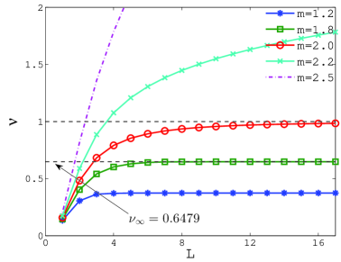
Figure 1: The dependence of the diffusion coefficient $\nu$ on the size $L$ of the support of the steady state for different exponents $m$. When $m>2$, $\nu$ increases indefinitely with $L$, while for $1<m\leq 2$, $\nu$ approaches a finite limit $\nu_{\infty}$ as $L\to\infty$ ($\nu_{\infty}=\|G\|_{L^{1}}$ for $m=2$ [12] and specified by (39) for $m<2$). The plot corresponds to the Gaussian kernel $G(x)=e^{-|x|^{2}/2}/\sqrt{2\pi}$, but the result seems to be generic for the class of potentials considered in this paper.

The steady states shown in Figure 2 exhibit qualitatively different behaviours too, depending on whether $1<m<2$ or $m>2$. We discuss the two cases separately.

Case $m>2$

When $m>2$ (see Figure 2(a)), the steady states are decreasing and concave down, and spread and decay to zero when $L$ increases to infinity. Moreover the numerical solution has a very peculiar form in this limit: it is close to a constant on the support, with a sharp drop near the boundary at $L$. Hence, for $L$ large, one can approximate the density profile by a rescaled characteristic function $\rho(x)\approx\frac{1}{2L}\chi_{[-L,L]}$ (to preserve unitary mass). Then $C=G*\rho(L)\approx 0$,

$$\frac{1}{2L}\int_{-L}^{L}G(x-y)dy\approx\frac{1}{2L}\|G\|_{L^{1}},$$

and the steady state equation (10) yields $(2L)^{1-m}\nu\approx(2L)^{-1}\|G\|_{L^{1}}$. This implies the scaling law

$$L\sim\nu^{1/(m-2)},\qquad\text{ for large }L.$$ (38)

A similar result, but regarding the dependence of $L$ on large mass (with $\nu$ fixed) was derived in [32].

To summarize, when $m>2$, for any diffusion coefficient $\nu>0$, there exists a compactly supported steady state that solves (10). Numerical results indicate that this steady state is unique and simulations of the evolution equation (1) (see Section 5) indicate that these equilibria are global attractors for the dynamics. The larger the diffusion coefficient $\nu$, the larger the size $L$ of the support, with scaling given by (38). Equilibria look like rescaled characteristic functions as $\nu$ (and $L$) become large.

   

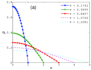
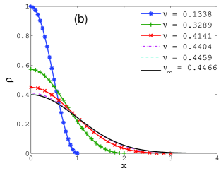
Figure 2: The steady states for the Gaussian kernel $G(x)=e^{-|x|^{2}/2}/\sqrt{2\pi}$ for (a) $m=2.2$ and (b) $m=1.5$, supported on domains of different sizes $L=1,2,3,4,5$ (the corresponding diffusion coefficients are shown in the legend). As $L$ increases to infinity the steady states approach a rescaled characteristic function when $m>2$, and converge to a fixed profile $\rho_{\infty}$ governed by (39) when $m\in(1,2)$. In the latter case, the steady state with $\nu=0.4459$ (or $L=5$) is indistinguishable from $\rho_{\infty}$ on the scale of the figure.

Case $1<m<2$

Solutions in this case (see Figure 2(b)) are also decreasing, but change concavity and reach the boundary $L$ of the support with zero derivative (results consistent with analytical considerations of Section 3.1).

Also in contrast with the previous case, the steady states approach a fixed profile as $L$ goes to infinity. We can identify this limiting profile as follows. As $L\to\infty$, $\nu$ approaches a constant value $\nu_{\infty}$ (Figure 1) and the constant $C$ in (10) approaches zero (see discussion on equilibria of infinite support in Section 2.3). Combing these observations, we infer from (10) that the limiting profiles $\rho_{\infty}$ are governed by the nonlinear eigenvalue problem

$$\nu_{\infty}\rho_{\infty}^{m-1}(x)=G*\rho_{\infty}(x),\qquad x\in\mathbb{R}.$$ (39)

In general, although no closed form expressions of the eigenpair $(\nu_{\infty},\rho_{\infty})$ are expected, (39) can be solved exactly for some special kernels $G$ like the Gaussian $e^{-|x|^{2}}/\sqrt{2\pi}$ or the Bessel potential $e^{-|x|}/2$.

We present the explicit calculation for the limiting profiles $\rho_{\infty}$ corresponding to the Gaussian kernel $G(x)=e^{-|x|^{2}}/\sqrt{2\pi}.$ For this kernel, the nonlinear eigenvalue problem (39) reads

$$\nu_{\infty}\rho_{\infty}(x)^{m-1}=\frac{1}{\sqrt{2\pi}}\int_{-\infty}^{\infty}e^{-(x-y)^{2}/2}\rho_{\infty}(y)dy,\qquad x\in\mathbb{R}.$$ (40)

We look for a solution in Gaussian form:

$$\rho_{\infty}(x)=e^{-x^{2}/2\sigma^{2}}/\sqrt{2\pi\sigma^{2}},$$

and by substituting into (40), we find

$$\sigma^{2}=\frac{m-1}{2-m},\qquad\nu_{\infty}=(2\pi)^{\frac{m}{2}-1}(m-1)^{\frac{m-1}{2}}(2-m)^{\frac{2-m}{2}}.$$

For $m=1.5$, $\nu_{\infty}\approx 0.4466$ and $\rho_{\infty}(x)=e^{-|x|^{2}/2}/\sqrt{2\pi}$, solution confirmed by numerics in Figure 2(b).

To conclude, when $m\in(1,2)$, solutions of (10) exist only for $\nu<\nu_{\infty}$. Numerics indicates that these solutions are unique, and simulations of the evolution equation (1) in Section 5 suggest that these equilibria are only local attractors for the dynamics. As $\nu$ approaches $\nu_{\infty}$ from below, the size $L$ of the support of solutions tends to infinity, and solutions approach a fixed density profile $\rho_{\infty}$. The pair $(\nu_{\infty},\rho_{\infty})$ solves (39). No compactly supported steady states exist for $\nu\geq\nu_{\infty}$. In such a case the evolution of (1) is dominated by diffusion and spreading to a trivial solution occurs.

4.3 Alternative Approach for the Bessel Potential $G(x)=e^{-|x|}/2$

For the Bessel potential $G(x)=e^{-|x|}/2$, in addition to using the general iterative scheme, various explicit calculations can be worked out by taking advantage of the fact that $G$ is the Green’s function of the differential operator $\operatorname{Id}-\partial_{xx}$. This special kernel has been already used in the study of steady states for $m=3$ in [32], as well as in various other nonlocal aggregation equations, including higher dimensional models [7, 25]. This alternative approach confirms that the qualitative behaviours for the Gaussian potential apply also to the Bessel potential, suggesting that the results are generic to all potentials in the class considered in this paper.

To this end, by symmetry of the solution, the equation (10) reads

$$\nu\rho(x)^{m-1}=\frac{1}{2}\int_{0}^{L}(e^{-|x-y|}+e^{-|x+y|})\rho(y)dy-C,\qquad x\in[0,L],$$ (41)

where

$$C=\frac{1}{2}\int_{0}^{L}(e^{-L-y}+e^{-L+y})\rho(y)dy.$$ (42)

Use the change of variable $p(x)=\rho(x)^{m-1}$ and apply the differential operator $\operatorname{Id}-\partial_{xx}$ to (41), to get

$$p-\frac{d^{2}p}{dx^{2}}=\frac{1}{\nu}\left(p^{\frac{1}{m-1}}-C\right),\qquad x\in[0,L],$$ (43)

with the boundary conditions $p^{\prime}(0)=0$ and $p(L)=0$. Note that we assume here that solutions have the properties considered in Section 3.1.

Multiplying both sides of (43) with $p_{x}$ and integrating with respect to $x$, one finds

$$\frac{1}{2}p^{2}-\frac{1}{2}p_{x}^{2}=\frac{m-1}{m\nu}p^{\frac{m}{m-1}}-\frac{C}{\nu}p+C_{1}.$$ (44)

Here the integration constant $C_{1}$ can be obtained from the conditions at the origin $p^{\prime}(0)=0$, i.e.,

$$C_{1}=\frac{1}{2}p(0)^{2}-\frac{m-1}{m\nu}p(0)^{\frac{m}{m-1}}+\frac{C}{\nu}p(0).$$

Solving $p^{\prime}(x)$ from (44) using the fact that $p^{\prime}(x)\leq 0$ on $[0,L]$, the solution can now be expressed implicitly as

$$x=\int_{p(x)}^{p(0)}\left[p^{2}-p(0)^{2}-\frac{2(m-1)}{m\nu}\big{(}p^{m/(m-1)}-p(0)^{m/(m-1)}\big{)}+\frac{2C}{\nu}\big{(}p-p(0)\big{)}\right]^{-1/2}dp,$$ (45)

where the size $L$ of the support is found from the condition $p(L)=0$:

$$L=\int_{0}^{p(0)}\left[p^{2}-p(0)^{2}-\frac{2(m-1)}{m\nu}(p^{m/(m-1)}-p(0)^{m/(m-1)})+\frac{2C}{\nu}(p-p(0))\right]^{-1/2}dp.$$ (46)

For fixed $\nu$, the problem of searching for the steady states is now reduced to finding the parameters $p(0)$ and $C$ such that the solution $\rho=p^{1/(m-1)}$ (depending on $p(0)$ and $C$) satisfies the constraints of unit mass and equation (42) for $C$.

This problem can be further simplified if instead of the unit mass condition we use the normalization $\bar{\rho}(0)=\bar{p}(0)=1$ for the solution. As explained in Section 3, a simple rescaling in the magnitude of the solution can be used to go between solutions with different types of normalizations. Hence, let $\bar{p}(x)$ be the solution defined implicitly by (45) (with $C$ replaced by $\bar{C}$) which satisfies $\bar{p}(0)=1$. By defining the function

$$I(\bar{C}):=\frac{1}{2}\int_{0}^{L}(e^{-L-y}+e^{-L+y})\bar{p}(y)^{1/(m-1)}dy,$$

we infer from (42) that $\bar{C}$ is a solution of the fixed point problem $I(\bar{C})=\bar{C}$. Notice that passing to the renormalization to unit mass, $\nu$ and $C$ have to be scaled along with $\rho$, i.e.,

$$\rho\to\frac{\bar{\rho}}{\int_{-L}^{L}\bar{\rho}(y)dy},\quad\nu\to\bar{\nu}\Big{(}\int_{-L}^{L}\bar{\rho}(y)dy\Big{)}^{m-2},\quad C\to\bar{C}\int_{-L}^{L}\bar{\rho}(y)dy,$$ (47)

with $\bar{\rho}=\bar{p}^{1/(m-1)}$.

When $\bar{\nu}$ is fixed and $\bar{p}(0)=1$, the interval on which we search for the fixed point of $I(\bar{C})$ is restricted by the requirement $\bar{p}^{\prime\prime}(0)\leq 0$ in (43) and by the non-negativity of the expression inside the square bracket in (45) at $p=0$. Both restrictions lead to upper bounds on $\bar{C}$, and can be written as

$$\bar{C}\leq\min\left(1-\bar{\nu},\frac{m-1}{m}-\frac{\bar{\nu}}{2}\right).$$ (48)

The function $I(\bar{C})$, shown in Figure 3(a) for $m=3$, has a fixed point only for $\bar{\nu}$ small enough (as indicated by (48)). An important observation is that the fixed point appears to be unique, consolidating our observation regarding unique solutions of (10).

   

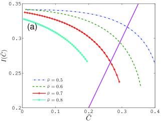
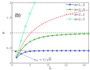
Figure 3: (a) The intersection of $I(\bar{C})$ with $\bar{C}$ for $m=3$ and different $\bar{\nu}$. (b) The dependence of $\nu$ on $L$ by finding the fixed point of $I(\bar{C})$ and rescaling to the unit mass normalization.

Rescaling the variables using the unit mass normalization (47), the dependence of $\nu$ on $L$ is shown in Figure 3(b). The result is similar to Figure 1, corresponding to the Gaussian kernel, and its interpretation follows closely the considerations made there.

The steady states computed from (43) are also similar to the corresponding equilibria for the Gaussian kernel (Figure 2), and are not shown here. When $m>2$, as $\nu$ increases to infinity, the convergence of the steady state to a rescaled characteristic function can be explained from a phase-plane analysis of the ODE (43) or the implicit equation (45). It can be shown (details not included) that in this limit, the coefficient $\nu$ and the constant $C$ relate in such a way that the solution $p(x)$ stays indeed very close to $p(0)$ for $x$ far away from the origin.

When $m\in(1,2)$, the limiting profiles $\rho_{\infty}$ can also be obtained explicitly, with $\nu_{\infty}$ solved from an algebraic equation. Using the vanishing condition $C=0$ and $\rho_{\infty}(\infty)\to 0$, the equation for $p_{\infty}=\rho_{\infty}^{m-1}$, when integrated once as in (44), becomes

$$\frac{1}{2}p_{\infty}^{2}-\frac{1}{2}p_{\infty}^{\prime 2}=\frac{m-1}{m\nu_{\infty}}p_{\infty}^{\frac{m}{m-1}}.$$ (49)

In particular, $p_{\infty}(0)=\big{(}\frac{m\nu_{\infty}}{2(m-1)}\big{)}^{(m-1)/(2-m)}$. As opposed to the general implicit equation (45), this equation can be integrated explicitly as

$$x=\int_{p_{\infty}(x)}^{p_{\infty}(0)}p^{-1}\left[1-\left(\frac{p}{p_{\infty}(0)}\right)^{\frac{2-m}{m-1}}\right]^{-1/2}dp=\frac{2(m-1)}{2-m}\mbox{arctanh}\sqrt{1-\left(\frac{p_{\infty}(x)}{p_{\infty}(0)}\right)^{\frac{2-m}{m-1}}}.$$

Therefore $\rho_{\infty}$ is then given by

$$\rho_{\infty}(x)=\left(\frac{m\nu_{\infty}}{2(m-1)}\right)^{1/(2-m)}\left[1-\tanh^{2}\frac{2-m}{2(m-1)}x\right]^{1/(2-m)},$$

where the constant $\nu_{\infty}$ is determined from the unit total mass, $\int_{\mathbb{R}}\rho_{\infty}(x)dx=1$. The exact value of $\nu_{\infty}$ can be obtained in a few cases, for instance, $\nu_{\infty}=1/\sqrt{6}$ when $m=3/2$ (see Figure 3(b)) and $\nu_{\infty}=(2\pi^{2})^{-1/3}$ when $m=4/3$.

Remark.

In higher dimensions, similar techniques involving the shooting method and a fixed point equation can be formulated to find the steady states, however the analogous equation to (15) for the derivative of the density does not seem to exist. As a result, there is no such iterative scheme as in section 4.1 to compute the steady states. This is the primary reason we focus on one dimension in this paper, although we expect similar qualitatively behaviours and demarcations at $m=2$. Among general kernels, the Bessel potentials are the very few cases when the corresponding steady states can be calculated without solving the evolution equation. The situation is however much more delicate in higher dimensions. It can be shown that, due to radial symmetry, the corresponding integral equation (8) in higher dimensions can be converted into the ODE

$$p-\frac{n-1}{r}\frac{dp}{dr}-\frac{d^{2}p}{dr^{2}}=\frac{1}{\nu}\big{(}p^{\frac{1}{m-1}}-C\big{)}.$$ (50)

Even though $m=2$ is still expected to be a critical exponent, there is no solution when $m$ is smaller than $m^{*}=2n/(n+2)$ or $1/(m-1)$ is larger than the critical Sobolev exponent $2^{*}-1=(n-2)/(n+2)$ in dimensions greater than two, at least for the limiting case [6] with $C=0$. Another complication is the singularity at the origin, which leads to blowup solutions when $m<2-2/n$ and the diffusion is not strong enough to balance the aggregation [24].

5 Dynamic Evolution

In this section we compute numerically the solutions to equation (1) to show that the steady states analyzed in the previous sections capture indeed the long time behaviour of the aggregation model.

5.1 Numerical Method

We use the numerical method recently developed in [15] to deal specifically with aggregation equations like (1), which contain interaction terms, nonlinear diffusion, and have a gradient flow structure. The method is based on a finite-volume scheme that preserves positivity and has the desired energy dissipation properties. We present briefly the method and for details we refer to [15].

We take a computational domain $[-L,L]$ with equally spaced grid points $-L=x_{0}<x_{1}<\cdots<x_{N}=L$. Consider the midpoints $x_{j-1/2}=(x_{j-1}+x_{j})/2$ and define $\bar{\rho}_{j}$ to be the average of the density on the cell $C_{j}=[x_{j-1/2},x_{j+1/2}]$. The finite volume method from [15] consists in a semi-discrete scheme in conservative form for $\bar{\rho}_{j}$:

$$\frac{d}{dt}\bar{\rho}_{j}(t)=-\frac{F_{j+1/2}(t)-F_{j-1/2}(t)}{\Delta x},$$ (51)

where $F_{j+1/2}$ approximates the continuous flux $\rho(G*\rho-\nu\rho^{m-1})_{x}$ at cell interfaces $x_{j+1/2}$.

The numerical fluxes $F_{j+1/2}$ are computed as follows. Consider the numerical approximations of the velocities at $x_{j+1/2}$:

$$u_{j+1/2}=(\xi_{j+1}-\xi_{j})/\Delta x,$$

where

$$\xi_{j}=\Delta x\sum_{k}G(x_{j}-x_{k})\bar{\rho}_{k}-\nu\bar{\rho}_{j}^{m-1}.$$

Then, the numerical flux $F_{j+1/2}$ is approximated by

$$F_{j+1/2}=u_{j+1/2}^{+}\rho_{j+1/2}^{+}+u_{j+1/2}^{-}\rho_{j+1/2}^{-},$$

where $u_{j+1/2}^{+}=\max(u_{j+1/2},0),u_{j+1/2}^{-}=\min(u_{j+1/2},0)$ and $\rho_{j+1/2}^{\pm}$ is the one-sided density at $x_{j+1/2}$ which depends on the spatial order of the scheme: $\rho_{j+1/2}^{+}=\bar{\rho}_{j+1},\rho_{j+1/2}^{-}=\bar{\rho}_{j}$ for first order and $\rho_{j+1/2}^{\pm}$ reconstructed from minmod or other slope-limiter for second order.

In all numerical examples the second order finite-volume method is used, while the system of (51) is integrated using the third-order strong-stability preserving Runge-Kutta method [19]. Despite its simplicity, this scheme preserves the positivity of the solution and dissipates the energy (see [15] for more details and extensive examples), which is critical for the study of long time behaviour of the solutions.

5.2 Asymptotic Behaviour and Metastability ($m>2$)

We evolve solutions to (1) in time and observe how they approach equilibria. To allow for a broad range of data, the initial densities are generated randomly as follows. First we generate density values on a coarse grid from the uniform distribution on the interval [0,1]. Then multiply everywhere with a Gaussian function of a certain width to ensure sufficient decay at the end of the intervals. Finally interpolate the density values on a fine grid and normalize to unit mass.

    

    

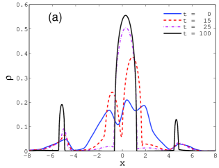
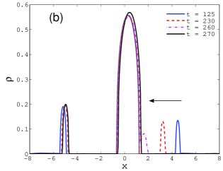
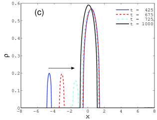
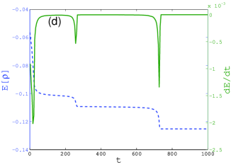
Figure 4: Dynamic evolution of (1) with $m=4$, $\nu=0.6$, and a Bessel attractive potential. Plot (a) demonstrates the coarsening of a randomly generated initial density. Plots (b) and (c) show the subsequent time evolution, with the smaller clumps eventually merging into the larger one. Plot (d) shows a staircase-like evolution of the energy (dashed line), along with the plot of its time derivative (solid line). The level regions of the energy correspond to metastable states consisting of multiple groups, while the sharp drops in $E$ and the peaks in its derivative $dE/dt$ correspond to group mergers.

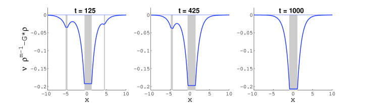
Figure 5: The plot of $\delta E/\delta\rho=\nu\rho^{m-1}-G*\rho$ at $t=125$, $t=425$ and $t=1000$ — see Figure 4. The graphs show that $\delta E/\delta\rho$ is constant on the different components of $\mathrm{supp}[\rho]$ (shaded regions). The (relatively weak) interaction between components is through the convolution $G*\rho$.

Figure 4(a)-(c) shows the time evolution of the solution of (1) for $m=4$, $\nu=0.6$ starting from such a randomly generated initial density ($t=0$ shown in plot Figure 3(a)). The attractive interaction kernel is the Bessel potential $G(x)=e^{-|x|}/2$. There is a fast coarsening of the initial density distribution resulting in three clumps (more clumps may appear for initial data with larger width), which eventually merge on a slow time scale.

The fast coarsening followed by slow group merging is characteristic to all simulations we performed, but it is more pronounced in the aggregation dominated regime of large $m$ (when $\rho(x,t)<1$) and small $\nu$. Our results are also consistent with numerical observations made in [32] using cubic nonlinearity ($m=3$).

To further understand this coarsening and metastability, it is very important to monitor dynamically the energy given by (3), shown in Figure 4(d). Note that after the initial coarsening, it decreases in a staircase fashion. A flat region corresponds to a multiple-clump configuration, which acts as a metastable state where the solution could spend a considerable amount of time. We chose to show this particular numerical simulation where the dynamics escapes the multiple-clump states rather fast, but we have seen cases where a multiple-clump state persists for a very long time. In fact, this delicate dynamics near a metastable state required the design of a suitable numerical scheme. Since the attractive kernels we use decay relatively fast with distance, once two groups get separated by a certain distance, they interact with each other very weakly and a long time may pass before their merger occurs. The sharp drops in the energy correspond to clump mergers. The closer clump on the right first merges with the large one in the center at around $t=265$. After the first merger, the two remaining clumps will persist for some time in a metastable configuration, before the left clump starts travelling to the right and merge with the central group. The second merger occurs at around $t=730$, corresponding to the second significant drop in energy. After that, the dynamics settles into the steady state identified and investigated in Sections 3 and 4.3.

One implication from these results is that there is no entropy-entropy dissipation inequality of the form

$$\frac{d}{dt}\big{(}E[\rho(\cdot,t)]-E[\rho(\cdot,\infty)]\big{)}\leq-\mu\big{(}E[\rho(\cdot,t)]-E[\rho(\cdot,\infty)]\big{)},$$

and the convergence of the solution $\rho(\cdot,t)$ to the steady state $\rho(\cdot,\infty)$ can be arbitrarily slow, in contrast to the fast convergence for other equations like the rescaled porous medium equation [16] or the Keller-Segel equation with subcritical mass [14].

The metastability can be understood from the plots of $\delta E/\delta\rho=\nu\rho^{m-1}-G*\rho$ shown in Figure 5. It is easy to see that, when the clumps are away from each other, $\delta E/\delta\rho$ is almost equal to a constant on each such component of the support of $\rho$ (shaded area), or $\partial_{x}(\delta E/\delta\rho)\approx 0$. Therefore, $\frac{d}{dt}E=-\int\rho|\partial_{x}(\delta E/\delta\rho)|^{2}\approx 0$, and this explains the level regions observed in Figure 4(d). When the clumps are far away from each other, the velocity of one particular clump is due to the nonlocal interaction kernel $G$, and decays as a function of distance between the other clumps in the same rate as $G$ [31]. In the extreme case of a compactly supported kernel $G$, steady states with multiple disconnected bumps do exist, where each such component is a locally stable steady state.

Coarsening, as well as metastability, are well-known phenomena in phase separation models [2], but are mainly studied in local systems with non-convex energy. Formation of metastable states in the case of nonlocal attraction has also been observed in chemotactic models [17, 13]. In these works the metastability was created by a doubly degenerate mobility, and indeed, in the zero diffusion limit, the metastable clusters became stable stationary solutions. In the case of the model we consider here, the metastability seems to be the result of a quasi-stationary energetic balance of attraction and repulsion, rather than being induced by mobility. A further analytical study of such effect seems to be a valuable subject for future research.

We conclude this subsection with a conjecture. Based on the numerical experiments and the theoretical results we conjecture that for $m>2$ the equilibria studied in Sections 3 and 4 are global attractors for the dynamics of (1). Note that in this regime a global minimizer of the energy (3)-(4) is known to exist [3].

5.3 Limited Basin of Attraction ($1<m<2$)

While the coarsening of the initial data and the metastability of the dynamics is still observed in this regime, the stronger diffusion (at least when the maximum density is less than one) leads to richer long time asymptotic behaviours. More precisely, the equilibria of Sections 3 and 4 are approached only when the diffusion coefficient is small enough ($\nu<\nu_{\infty}$) and the initial data is localized near its center of mass.

  

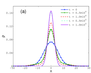
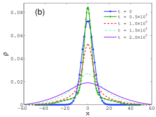
Figure 6: Different long time behaviours of the solution for $m=1.8$. Here $G(x)=e^{-|x|^{2}/2}/\sqrt{2\pi}$, $\nu=0.60<\nu_{\infty}\approx 0.6479$ and the initial data is a Gaussian $u_{0}(x)=e^{-|x|^{2}/2\sigma^{2}}/\sqrt{2\pi\sigma^{2}}$ ($\sigma^{2}=30$ in (a) and $\sigma^{2}=50$ in (b)). The solution converges either to the compactly supported steady state or to the trivial solution, depending on the spread of the initial profile.

The dynamic evolution for two Gaussian initial profiles with different widths for $m=1.8$, $\nu=0.60$ and $G(x)=e^{-|x|^{2}}/\sqrt{2\pi}$ is shown in Figure 6. Although the compactly supported steady state exists ($\nu<\nu_{\infty}\approx 0.6479$), the solution converges to this stationary solution only when the width of the initial data is small enough; otherwise the solution spreads and decays to a trivial state. The steady states of Sections 3 and 4 are only local attractors for the dynamics. The decaying solution with large width can be explained formally by the long wave approximation $G*\rho(x)\approx\|G\|_{L^{1}}\rho(x)$, where the original equation (1) becomes

$$\partial_{t}\rho=\partial_{x}\big{(}\rho\partial_{x}(\nu\rho^{m-1}-\rho\|G\|_{L^{1}})\big{)}.$$ (52)

For small densities, the diffusion arising from $\nu\rho^{m-1}$ dominates the anti-diffusion from $\rho\|G\|_{L^{1}}$, and the solution continues to decay to zero.

  

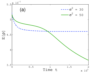
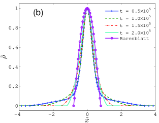
Figure 7: (a) Time decay of the energy corresponding to the simulations from Figure 6. (b) Rescaled profiles of the spreading solution in Figure 6(b) approach asymptotically a rescaled Barenblatt profile.

Compared with the case $m>2$, another fundamental difference when $m\in(1,2)$ is the fact that the energy corresponding to the compactly supported steady state can be positive when $\nu$ is close to $\nu_{\infty}$. Figure 7(a) shows the evolution of the energy corresponding to the two dynamic simulations from Figure 6. The solution with small initial width converges to a positive energy, while the solution with large initial width that decays to zero has energy that goes to zero as well. In particular, at $\nu=\nu_{\infty}$ the steady state is governed by (39) and $E[\rho_{\infty}]=(\frac{1}{m}-\frac{1}{2})\nu_{\infty}\int(\rho_{\infty})^{m}>0$. This observation once again confirms that for $\nu$ near the critical diffusion $\nu_{\infty}$, the compactly supported steady states can only be local minimizers. It is possible that they turn into global minimizers once $\nu$ drops below a certain threshold (strictly smaller than $\nu_{\infty}$), but this aspect will be investigated elsewhere.

When the solution spreads and decays to zero, the dynamics is expected to be dominated by the nonlinear diffusion [4]. For the decaying solution from Figure 6(b), the rescaled profiles $\tilde{\rho}(\tilde{x},t)=\lambda^{-1}\rho(\lambda^{-1}\tilde{x},t)$ with $\lambda=\max_{x}\rho(x,t)$ shown in Figure 7(b) converge indeed to the rescaled Barenblatt profile, the solution of the porous medium equation $\rho_{t}=\nu\partial_{x}(\rho\partial_{x}\rho^{m-1})$. The convergence however seems slow and is established only for very large time.

Appendix A Proof of the last fact about equilibria in Section 2.3

Lemma A.1.

Let $\rho$ be a stationary solution of (2) in one dimension, with compact support. Then there exists a symmetric stationary solution $\widetilde{\rho}$ such that

$$E[\widetilde{\rho}]=E[\rho].$$

Proof.

Let $\mathrm{supp}[\rho]=[a,b]$ for some $a,b\in\mathbb{R}$. For a given $x\in(a,b)$ we have

$$\nu f(\rho(x))=G*\rho(x)+C$$ (53)

for some $C\in\mathbb{R}$. Evaluation on $x=a$ and $x=b$ gives

$$C=-\int_{a}^{b}G(a-y)\rho(y)dy=-\int_{a}^{b}G(b-y)\rho(y)dy.$$

Let $\overline{\rho}(x)=\rho(x+x_{0})$ with $x_{0}=(a+b)/2$. Then $\overline{\rho}$ is still a steady state and it satisfies $E[\overline{\rho}]=E[\rho]$ due to translation invariance. Moreover, the support of $\overline{\rho}$ is symmetric. Let us introduce

$$\widetilde{\rho}(x):=f^{-1}\left(\frac{1}{2}(f(\overline{\rho})(x)+f(\overline{\rho})(-x))\right).$$

Clearly, $\mathrm{supp}[\widetilde{\rho}]=\mathrm{supp}[\overline{\rho}]$ and we have, for all $x\in\mathrm{supp}[\widetilde{\rho}]$,

$$\nu f(\widetilde{\rho}(x))=\frac{\nu}{2}(f(\overline{\rho}(x))+f(\overline{\rho}(-x)))=\frac{\nu}{2}(f(\rho(x+x_{0}))+f(\rho(-x+x_{0})))$$

$$\ =\frac{1}{2}\int_{a}^{b}G(x+x_{0}-y)\rho(y)dy+\frac{1}{2}\int_{a}^{b}G(-x+x_{0}-y)\rho(y)dy+C$$

$$\ =\frac{1}{2}\int_{(a-b)/2}^{(b-a)/2}G(x-z)\overline{\rho}(z)dy+\frac{1}{2}\int_{(a-b)/2}^{(b-a)/2}G(-x-z)\overline{\rho}(z)dy+C$$

$$\ =\frac{1}{2}\int_{(a-b)/2}^{(b-a)/2}G(x-z)\overline{\rho}(z)dy+\frac{1}{2}\int_{(a-b)/2}^{(b-a)/2}G(x-z)\overline{\rho}(-z)dy+C$$

$$\ =\int_{(a-b)/2}^{(b-a)/2}G(x-z)\frac{1}{2}\left(\overline{\rho}(z)+\overline{\rho}(-z)\right)dz+C=\int_{(a-b)/2}^{(b-a)/2}G(x-z)\widetilde{\rho}(z)dz+C$$

where we have used the symmetry of $G$. The above computation shows that $\widetilde{\rho}$ has the same energy as $\rho$ . ∎

References

- [1] L. Ambrosio, N. Gigli, and G. Savaré. Gradient flows in metric spaces and in the space of probability measures. Lectures in Mathematics ETH Zürich. Birkhäuser Verlag, Basel, second edition, 2008.
- [2] P. Bates and J. Xun. Metastable patterns for the Cahn-Hilliard equation I. J. Differential Equations, 111(2):421–457, 1994.
- [3] J. Bedrossian. Global minimizers for free energies of subcritical aggregation equations with degenerate diffusion. Appl. Math. Lett., 24(11):1927–1932, 2011.
- [4] J. Bedrossian. Intermediate asymptotics for critical and supercritical aggregation equations and Patlak-Keller-Segel models. Commun. Math. Sci., 9(4):1143–1161, 2011.
- [5] J. Bedrossian, N. Rodríguez, and A. L. Bertozzi. Local and global well-posedness for aggregation equations and Patlak-Keller-Segel models with degenerate diffusion. Nonlinearity, 24:1683–1714, 2011.
- [6] H. Berestycki and P.-L. Lions. Nonlinear scalar field equations. I. Existence of a ground state. Arch. Rational Mech. Anal., 82(4):313–345, 1983.
- [7] A. J. Bernoff and C. M. Topaz. A primer of swarm equilibria. SIAM J. Appl. Dyn. Syst., 10(1):212–250, 2011.
- [8] A. L. Bertozzi and D. Slepčev. Existence and uniqueness of solutions to an aggregation equation with degenerate diffusion. Commun. Pure Appl. Anal., 9(6):1617–1637, 2010.
- [9] A. Blanchet, J. A. Carrillo, and P. Laurençot. Critical mass for a Patlak-Keller-Segel model with degenerate diffusion in higher dimensions. Calc. Var. Partial Differential Equations, 35(2):133–168, 2009.
- [10] M. Burger, V. Capasso, and D. Morale. On an aggregation model with long and short range interactions. Nonlinear Analysis: Real World Applications, 8:939–958, 2007.
- [11] M. Burger and M. Di Francesco. Large time behavior of nonlocal aggregation models with nonlinear diffusion. Netw. Heterog. Media, 3(4):749–785, 2008.
- [12] M. Burger, M. Di Francesco, and M. Franek. Stationary states of quadratic diffusion equations with long-range attraction. Comm. Math. Sci., 3, 2013. To appear.
- [13] M. Burger, Y. Dolak-Struss, and C. Schmeiser. Asymptotic analysis of an advection-dominated chemotaxis model in multiple spatial dimensions. Commun. Math. Sci., 6(1):1–28, 2008.
- [14] V. Calvez and J. A. Carrillo. Refined asymptotics for the subcritical keller-segel system and related functional inequalities. Proceedings of the American Mathematical Society, 140(10):3515–3530, 2012.
- [15] J. Carrillo, A. Chertock, and Y. Huang. A finite volume method for nonlinear diffusion equations with a gradient flow structure. 2013. In preparation.
- [16] J. A. Carrillo and G. Toscani. Asymptotic l1-decay of solutions of the porous medium equation to self-similarity. Indiana University Mathematics Journal, 49(1):113–142, 2000.
- [17] Y. Dolak and C. Schmeiser. The Keller-Segel model with logistic sensitivity function and small diffusivity. SIAM J. Appl. Math., 66(1):286–308, 2005.
- [18] H. W. Engl. Integralgleichungen. Springer Lehrbuch Mathematik. [Springer Mathematics Textbook]. Springer-Verlag, Vienna, 1997.
- [19] S. Gottlieb, C.-W. Shu, and E. Tadmor. Strong stability-preserving high-order time discretization methods. SIAM Rev., 43:89–112, 2001.
- [20] D. Grünbaum and A. Okubo. Modelling social animal aggregations. In S. A. Levin, editor, Frontiers in mathematical biology, Lecture notes in biomathematics 100, pages 296–325. Springer-Verlag, Berlin Heidelberg, 1994.
- [21] M. E. Gurtin and A. C. Pipkin. A note on interacting populations that disperse to avoid crowding. Quart. Appl. Math., 42(1):87–94, 1984.
- [22] T. Ikeda. Standing pulse-like solutions of a spatially aggregating population model. Jpn. J. Appl. Math., 2:111–149, 1985.
- [23] T. Ikeda and T. Nagai. Stability of localized stationary solutions. Jpn. J. Appl. Math., 4:73–97, 1987.
- [24] H. Kozono and Y. Sugiyama. Local existence and finite time blow-up of solutions in the 2-D Keller-Segel system. J. Evol. Equ., 8:353–378, 2008.
- [25] A. J. Leverentz, C. M. Topaz, and A. J. Bernoff. Asymptotic dynamics of attractive-repulsive swarms. SIAM J. Appl. Dyn. Syst., 8(3):880–908, 2009.
- [26] H. Li and G. Toscani. Long-time asymptotics of kinetic models of granular flows. Arch. Ration. Mech. Anal., 172(3):407–428, 2004.
- [27] P. A. Markowich and C. Villani. On the trend to equilibrium for the Fokker-Planck equation: an interplay between physics and functional analysis. Mat. Contemp., 19:1–29, 2000. VI Workshop on Partial Differential Equations, Part II (Rio de Janeiro, 1999).
- [28] A. Mogilner and L. Edelstein-Keshet. A non-local model for a swarm. J. Math. Biol., 38(6):534–570, 1999.
- [29] D. Morale, V. Capasso, and K. Oelschläger. An interacting particle system modelling aggregation behavior: from individuals to populations. J. Math. Biol., 50(1):49–66, 2005.
- [30] T. Nagai and M. Mimura. Asymptotic behavior for a nonlinear degenerate diffusion equation in population dynamics. SIAM J. Appl. Math., 43:449–464, 1983.
- [31] D. Slepcev. Coarsening in nonlocal interfacial systems. SIAM Journal on Mathematical Analysis, 40(3):1029–1048, 2008.
- [32] C. M. Topaz, A. L. Bertozzi, and M. A. Lewis. A nonlocal continuum model for biological aggregation. Bull. Math. Bio., 68:1601–1623, 2006.