Effects of Lyman alpha scattering in the IGM on clustering statistics of Lyman alpha emitters

We investigate the correlations between the observed fraction of Ly$\alpha$ emission from star-forming galaxies and the large scale structure by post-processing snapshots of a large, high resolution hydrodynamical simulation with a Ly$\alpha$ radiative transfer code at redshifts $z=4,\;3,\;2$. We find correlations of the observed fraction with density, density gradient along the line of sight, velocity and velocity gradient along the line of sight, all within the same order of magnitude (tens of percent). Additionally, a correlation with the angular momentum of the dark matter halo is detected. In contrast to a previous study, we find no significant deformation of the 2-point correlation function due to selection effects from radiative transfer in the IGM within the limited statistics of the simulation volume.

1 Introduction

Galaxies with strong Ly$\alpha$ emission features, so-called Ly$\alpha$ emitters (LAEs), are powerful probes of galaxy evolution and cosmological large scale structure. There are indications that LAEs, or some subset thereof, evolved into today’s Milky Way type galaxies (Guaita et al., 2010), hence their properties may shed light on our own galaxy’s youth. Also, future observations might be able to detect the first galaxies via Ly$\alpha$ emission (e.g Dijkstra & Wyithe, 2010).

LAEs can be detected very efficiently in narrow-band or integral-field spectrographic surveys such as the Hobby-Eberly Telescope Dark Energy Experiment (HETDEX) (Adams et al., 2011). They have been proposed to act as tracers of the underlying matter distribution at higher redshifts than currently accessible for galaxy redshift surveys. Specifically, HETDEX aims to use the power spectrum of $\sim$ 800.000 LAEs to measure the Hubble parameter $H(z)$ and angular distance $D_{A}(z)$ at redshifts between $z=1.9$ and 3.5 with percent-level accuracy in order to constrain the early dynamics of dark energy.

Every interpretation of LAE observations needs to take into account the resonant nature of Ly$\alpha$ scattering (e.g. Cantalupo et al., 2005; Dijkstra et al., 2006; Adams et al., 2009; Zheng et al., 2010; Yajima et al., 2012; Schaerer et al., 2011; Hansen & Peng Oh, 2006). The large cross section of Ly$\alpha$ photons scattering with neutral hydrogen strongly correlates the observed Ly$\alpha$ spectra and apparent luminosities along any given line-of-sight with the density and velocity structure of the intervening HI (Dijkstra et al., 2006; Laursen et al., 2011). As a result, large amounts of information are encoded in the observations. On scales of the emitting galaxies and their circumgalactic material, Ly$\alpha$ spectra are very sensitive to the presence of clumps, dust, and in- or outflows (Zheng & Miralda-Escude, 2002; Dijkstra et al., 2006; Laursen et al., 2009b; Schaerer et al., 2011; Barnes et al., 2011). Recent simulations also highlight the possibility of a strong inclination dependence of the Ly$\alpha$ observed fraction which, in turn, depends on the morphology of the gaseous disk (Laursen & Sommer-Larsen, 2007; Yajima et al., 2012; Verhamme et al., 2012). Mapping the theoretical predictions, mostly from numerical simulations, to properties of observed LAEs has only just begun (e.g. Nagamine et al., 2010; Shimizu et al., 2011; Forero-Romero et al., 2011; Dayal & Ferrara, 2012) and promises to be a rich field of research in the coming years.

On the other hand, correlations of apparent LAE luminosities with the matter distribution induced by Ly$\alpha$ radiation transport (RT) effects can also contaminate the clustering statistics of LAEs on larger scales. If they reach out to scales relevant for the extraction of cosmological parameters, they need to be accounted for by corrections in the LAE power spectrum in real and redshift space. This effect was demonstrated by Zheng et al. (2011a) (ZCTM11) using a Monte-Carlo Ly$\alpha$ RT calculation on the background of a cosmological simulation snapshot at $z=5.7$. Details of their setup and further investigations with regards to the luminosity, spectra and observed fractions of LAEs in their simulation can be found in Zheng et al. (2010) (ZCTM10) (see also Zheng et al. (2011b) for details on extended LAE halos). They found significant correlations of the Ly$\alpha$ observed fraction, i.e. the fraction of photons that are not scattered out of the line-of-sight during their passage through the intergalactic medium (IGM), with the smoothed IGM density and velocity fields. By far the biggest effect was seen in correlations with the velocity gradient field, accompanied by a strongly anisotropic signature in the 2-point correlation function for LAEs in redshift space. If present also at lower redshifts, an effect of this magnitude would seriously affect the interpretation of LAE large-scale structure surveys like HETDEX. This was investigated in more detail in Wyithe & Dijkstra (2011) by means of analytic and numerical models for LAE spectra with in- and outflows, which the authors used to calibrate a modified parametrization for the LAE power spectrum. Using an Alcock-Paczynski test, they then showed that the accuracy of HETDEX measurements could potentially be seriously compromised by Ly$\alpha$ RT effects. In Greig et al. (2012), this analysis was extended to include the LAE bispectrum which allows to break the degeneracy between Ly$\alpha$ RT effects and gravitational redshift-space distortion that is present at the level of the power spectrum alone.

While being the most extensive numerical investigation of Ly$\alpha$ RT on cosmological scales, the methodology and resolution of the simulation analyzed by ZCTM10/11 were inadequate to capture the nonlinear hydrodynamics in the circumgalactic medium (CGM) surrounding LAEs. Instead of a full hydrodynamical simulation, ZCTM10/11 employed a hybrid scheme which assumed hydrostatic equilibrium for the gas in virialized halos. Consequently, no outflows were present in their simulation, and the infall was purely gravitational with no hydrodynamical modifications on CGM scales. In Wyithe & Dijkstra (2011), galactic outflows were modeled in a simplified way that was also assumed to be independent of the environment on linear scales. The exact degree to which nonlinear flows on scales $\lesssim 100$ kpc are correlated with their large-scale environment is still unclear, but can plausibly be assumed to be non-vanishing. In this case, the well-known strong sensitivity of LAE properties on CGM/IGM flows (e.g. Dijkstra et al., 2007; Iliev et al., 2008; Laursen et al., 2011) will be reflected to some extent in the large-scale statistics. Including the effects of fully hydrodynamical in- and outflows was one of the main motivations for this work.

Another question raised by ZCTM10/11 is the redshift dependence of the observed correlations. This is particularly important for HETDEX which will cover a redshift range which is significantly below the one explored by ZCTM10/11.

In this work, we revisit the the analysis of ZCTM10/11 using Ly$\alpha$ RT on the background of snapshots of the MareNostrum-Horizon simulation (Ocvirk et al., 2008) at redshifts of $z=2,3$ and 4. The MareNostrum simulation has a spatial resolution of 1 kpc (physical) and includes a model for supernova feedback driving galactic outflows in a self-consistent fashion. In addition to evaluating the correlations of the Ly$\alpha$ observed fraction with the IGM density and velocity on linear scales, we tested for a possible dependence on the orientation of the halos’ angular momentum relative to the line-of-sight, serving as a proxy for the orientation of the galactic disk. We find a positive result, indicating that tidal alignment of halos might give rise to additional spurious signals in redshift space distortions (Hirata, 2009).

Our numerical techniques for Ly$\alpha$ RT are summarized in Sec. B of the appendix. We describe the details of the simulation and our postprocessing runs in Sec. 2. Our results for the correlations of large-scale density and velocity fields with Ly$\alpha$ observed fractions are presented in Sec. 4.

2 Ly$\alpha$ Radiation Transport Calculations and Analysis

2.1 The Horizon-MareNostrum Galaxy Formation Simulation

We applied our radiative transfer code LyS (see the appendix for details) to snapshots taken from the Horizon-MareNostrum Galaxy Formation run which was presented and described in Ocvirk et al. (2008). The simulation was run using an updated version of the AMR code Ramses (Teyssier, 2002), including metal dependent cooling, star formation, a simple supernova feedback model and UV heating. The box had a comoving size of 50 Mpc/h with a physical resolution of 1 kpc. Star formation took place in the interstellar medium (ISM), defined as gas with a number density greater than 0.1 $n_{H}$/cm³. The dark matter particle mass was $8\times 10^{6}$ M_⊙ with a total particle count of $1024^{3}$. The simulation was run assuming a standard $\Lambda$CDM cosmology with $\Omega_{M}$ = 0.3, $\Omega_{\Lambda}$ = 0.7, $\Omega_{B}$ = 0.045, $H_{0}$ = 70 km/s/Mpc and $\sigma_{8}$ = 0.9. For more information on the spectroscopic properties of galaxies in the simulation, see Gay et al. (2009).

2.2 Preprocessing

We rebuilt the AMR hierarchy of the MareNostrum run and calculated the temperatures of the gas cells from the specific pressure assuming photoionization equilibrium (Katz et al., 1996). In the ISM regions, the breakdown of single component fluid description leads to artificially high temperatures. To overcome this problem, we enforce an upper limit of 2.5 $\times 10^{4}$ K on the ISM temperature.

In order to find the emission spots for the Lyman-$\alpha$ photons, we used the HOP algorithm (Eisenstein & Hut, 1998) to produce a halo list. We used a standard set of parameters ($\delta_{outer}=80,\delta_{saddle}=200,\delta_{peak}=240$) and rejected particles groups that consist of less than 600 particles after the regrouping process, corresponding to a cut-off mass of $4.8\times 10^{9}M_{\odot}$. With this cut-off, we have a sample size of $\sim$ 42.000/49.000/51.000 emitters at redshift 4/3/2. The mass range of these emitters is 5 $\times 10^{9}$ M_⊙ to 3.1 $\times 10^{12}$/8.0 $\times 10^{12}$/3.3 $\times 10^{13}$ M_⊙ for $z=4/3/2$.

3 Our Simulations and Analysis

The Ly$\alpha$ RT was run as a postprocessing step on simulation snapshots at redshift $z=2,3$ and 4. Additionally to the fiducial case, we re-ran our simulation at redshift 4 with a) the Hubble flow, b) the peculiar velocity field and c) both turned off for interpretation and comparison. To achieve this, we set the Hubble constant in eq. 18 to zero and/or set the total bulk velocity $v$ in eq. 11 to zero so that the restframe of each gas cell is identical to the restframe of the emitter. The thermal motion of the gas is however not affected by this procedure. We also ran the redshift 4 snapshot along three different lines of sight. For details on the initialization of spectra and luminosities, we refer the reader to Sec. B. The spatial resolution of our output array is 16.3 kpc/h (comoving), corresponding to 0.67/0.74/0.91” at redshift 4/3/2.

The output matrix was converted into physical fluxes and surface brightnesses. By integrating over the spectral information of the output matrix, we obtained surface brightnesses of each $(i_{y},i_{z})$-pixel. For each halo, we ran a friend-of-friend algorithm to find the apparent luminosity of the source. If the pixel covering the central position of the halo had a surface brightness exceeding a threshold $\eta$, we added its flux to the flux of the source, and connected adjacent pixels that are above the threshold.

Using the total flux of each source obtained with this procedure, we defined the source’s inferred apparent luminosity

$L_{apparent}$. As a result, we can compute the fraction

$$\epsilon=\frac{L_{apparent}}{L_{intrinsic}}$$ (1)

of the intrinsic luminosity that was detected. Since this quantity measures the part of the intrinsic luminosity that an observer would see, it plays the role of an observed fraction, and hereafter we will refer to it by this term. We caution the reader that in our case, the difference between intrinsic and inferred luminosity is not due to destruction of photons by dust, but due to the application of a detection limit.

To prevent source blending, we identified and ignored sources that would swallow up other emitters during the post-processing, although these blended source are quite rare ($\sim$ 5% of the total number) and did not affect our results very much.

The chosen value of the surface brightness limit $\eta$ is somewhat arbitrary because we didn’t include dust and did not model the systematic errors of a real observation in detail. We used a value similar as ZCTM10:

$$\eta=5\times 10^{-19}\textrm{erg s}^{-1}\textrm{cm}^{-2}\textrm{arcsec}^{-2}$$ (2)

This particular value was chosen to be well above the noise level in the output data. We caution the reader that this threshold is orders of magnitude smaller than the detection threshold of e.g. HETDEX, which is $\eta\simeq 10^{-17}\textrm{erg s}^{-1}\textrm{cm}^{-2}\textrm{arcsec}^{-2}$. We chose a lower value in order to be comparable with ZCTM10 but also not to degrade statistics by having only few sources detected.

The observed fraction of Ly$\alpha$ along a specific line of sight is related to the density and velocity structure along the line of sight (Wyithe & Dijkstra, 2011) (note that ZCTM10 and ZCTM11 stress the importance of the structure in the perpendicular directions). In order to find the correlations between the dark matter distribution in the MareNostrum simulation and the observed fractions on linear scales relevant for LAE redshift surveys, we closely followed the strategy described by ZCTM10. The dark matter particles were interpolated onto a grid using a cloud-in-cell algorithm and smoothed out on a scale of 10/12/15 Mpc/$h$ with a top-hat filter of this diameter. We chose this filtering scale to obtain the density field in the linear regime at redshift 4/3/2 consistent with our calculations below. From the smoothed density field, we calculated the linear velocity field and density/velocity gradients along the line of sight.

The smoothed density and velocity fields are well described by linear theory. From the continuity equation

$$\dot{\delta}=-\frac{1}{a}div\;\@vec{u}$$ (3)

one finds the peculiar velocity field $\@vec{u}_{k}$ in Fourier space:

$$\@vec{u}_{k}=fHa\frac{i\@vec{k}}{k^{2}}\delta_{k}$$ (4)

We are only interested in the line of sight component of the velocity field which we assume to be parallel to the $x$-axis here:

$$u_{x}=fHa\sum_{\@vec{k}}\frac{k_{x}i}{k^{2}}\delta_{k}e^{i\@vec{k}\cdot\@vec{r}}\,\,.$$ (5)

The spatial derivative of the velocity field in the line of sight is given by

$$\frac{\partial u_{x}}{\partial x}=-fHa\sum_{\@vec{k}}\frac{k_{x}^{2}}{k^{2}}\delta_{k}e^{i\@vec{k}\cdot\@vec{r}}\,\,.$$ (6)

We also calculate the angular momentum of the individual halos directly from the particle data.

4 Results

4.1 Overview

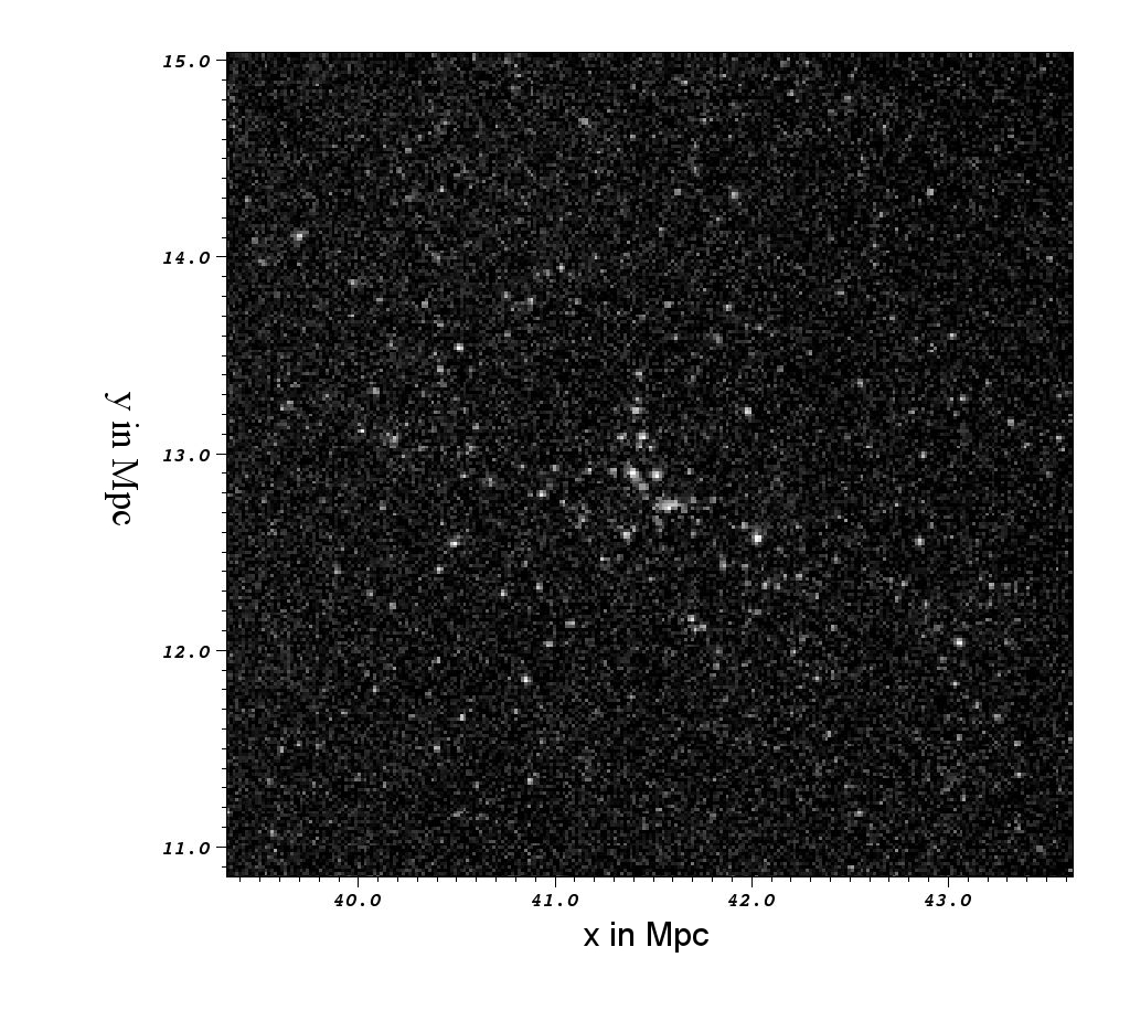
Figure 1: Lyman-$\alpha$ image of a small part ($\sim$5 $\times$ 5 Mpc) of the simulation volume at redshift 4. The observer is located along the positive $z$-axis, the snapshot corresponds to $z=4$.

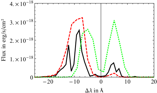
Figure 2: Typical Spectrum of an emitter with a mass of 1.9 $\times$ 10¹⁰ M_⊙. Shown is the spectrum for the fiducial simulation (solid line), the simulation without any peculiar velocities and Hubble flow (dotted line), and a simulation where peculiar velocities were enabled but the Hubble flow was switched off (dashed line). Wavelength is given with respect to the observer’s restframe. For the fiducial simulation, the redshift due to the Hubble flow within the simulation box was ignored.

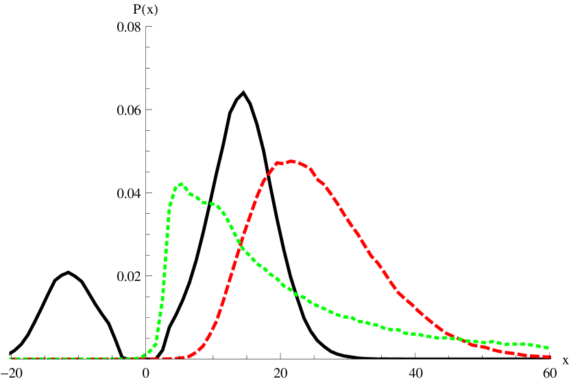
Figure 18: Shown is the dimensionless frequency distribution of photons escaping from an isothermal ($2\times 10^{4}$ K) homogeneous sphere with an column density of $2\times 10^{20}$ $N_{H}$ from the center to the surface. A Hubble-like velocity prescription given by eq. 24 is assigned. The different lines correspond to different maximum collapse velocities: 20 km/s (line), 200 km/s (dashed), 2000 km/s (dotted).

Figure 1 shows a spectrally integrated image of the LAEs in the box as seen by an observer located along the positive $z$-axis. In fig. 2, the spatially integrated spectrum of an emitter with a mass of $1.9\times 10^{10}$ M_⊙ is shown for three different setups: the solid line shows the spectrum of the fiducial run, the dotted line shows a run with all peculiar motions and the Hubble flow artificially set to zero, and the dashed line is obtained from a simulation where only the Hubble flow was switched off. For the case without peculiar motions and Hubble flow, we clearly see the typical double-peaked spectrum that one would get from a static sphere (see fig. 17). Deviations from this solution result from anisotropic density fields. Turning on the velocity field, we obtain the typical spectrum of an infalling sphere (see fig. 18) which is intuitive since the region in the halo’s vicinity should show clear infall. Photons are thereby shifted to the blue side of the spectrum, undergoing only few scatterings after leaving the halo. If we switch on the Hubble flow, the situation changes. Blue photons leaving the ISM are shifted back into the line center and scattered in the intervening IGM. As a consequence, the observed flux is significantly reduced because photons are scattered out of the line of sight. We note again that these photons are not destroyed by dust but they contribute to a noise level of diffuse emission. The Hubble flow transports photons from the blue to the red side of the spectrum. Once photons have left the line center to the red side they will be further redshifted, making subsequent scatterings more and more improbable.

The surface brightness profiles for two sources are shown in fig. 4. It is worth noting that while ZCTM10 reported extended Ly$\alpha$ halos (r $\sim$ 300 kpc) with surface brightnesses of $\sim$ 10^-20 $\textrm{erg s}^{-1}\textrm{cm}^{-2}\textrm{arcsec}^{-2}$ at $z=5.7$ we find rather compact sources. These differences might be partly attributed to the lower redshift in our simulation. Additionally, as we resolve the ISM at least marginally, most of the scatterings happen in the ISM where the optical depth is high due to high HI densities. This shifts the photons out of resonance and reduces the optical depth of the immediate surroundings of the halo. Since later IGM scatterings happen far away from the emitting halo, they contribute to a diffuse background rather than to an extended Ly$\alpha$ halo.

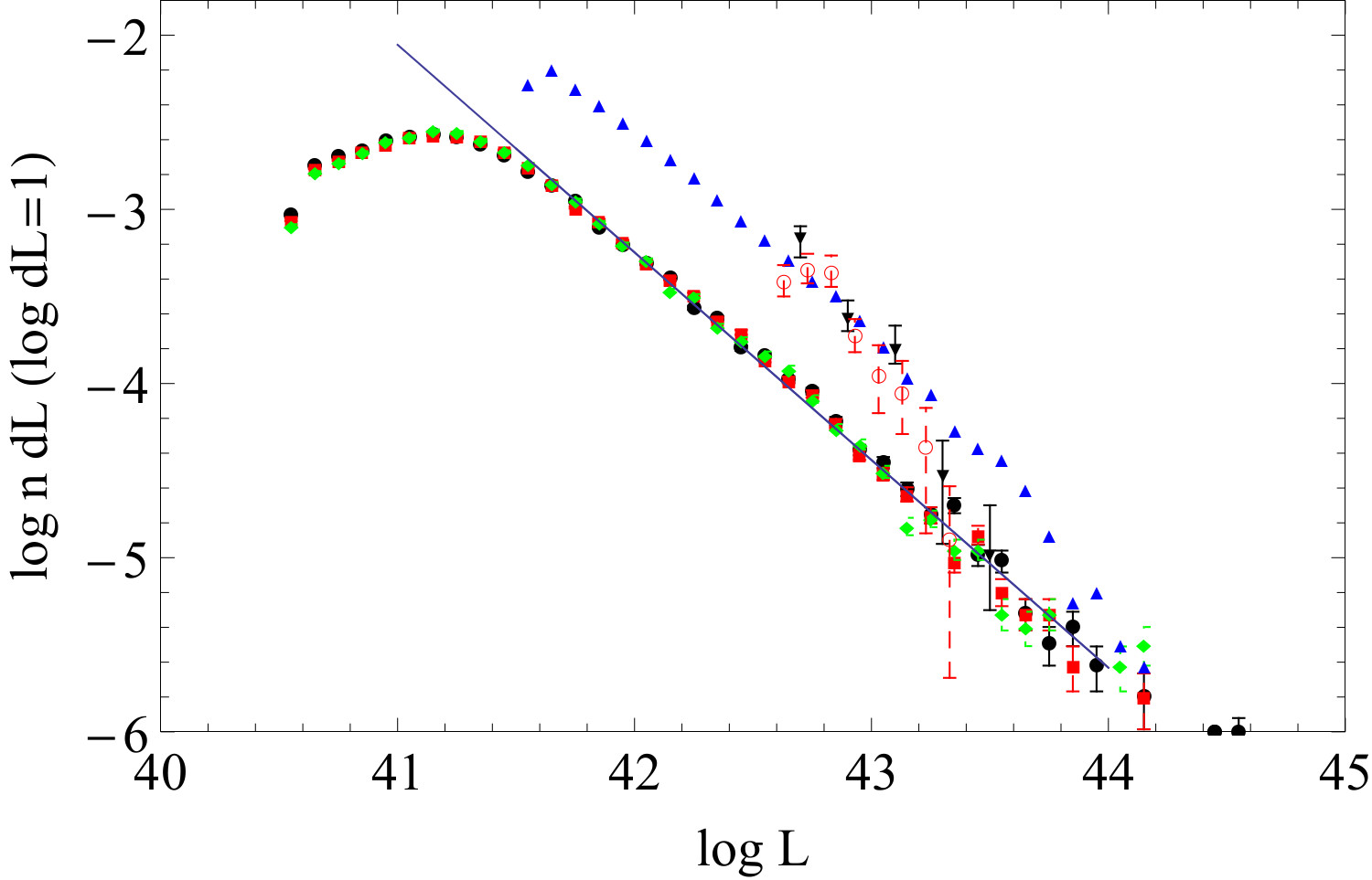
Figure 3: Luminosity function from our simulation at $z=4$ for three different lines of sight. The observer is set along the x-axis (circles), y-axis (boxes) and z-axis (diamonds), respectively. Triangles without error bars show the distribution of the intrinsic luminosity. Hollow circles show the observed luminosity function for $z=4.5$ (Wang et al., 2009), the flipped triangles show the luminosity function for $z=3.7$ as observed by Ouchi et al. (2008). The line depicts the log-linear fit to the data, yielding a power law with $\alpha=-1.19$. Number density is in units of Mpc${}^{-3}/\log(L)$.

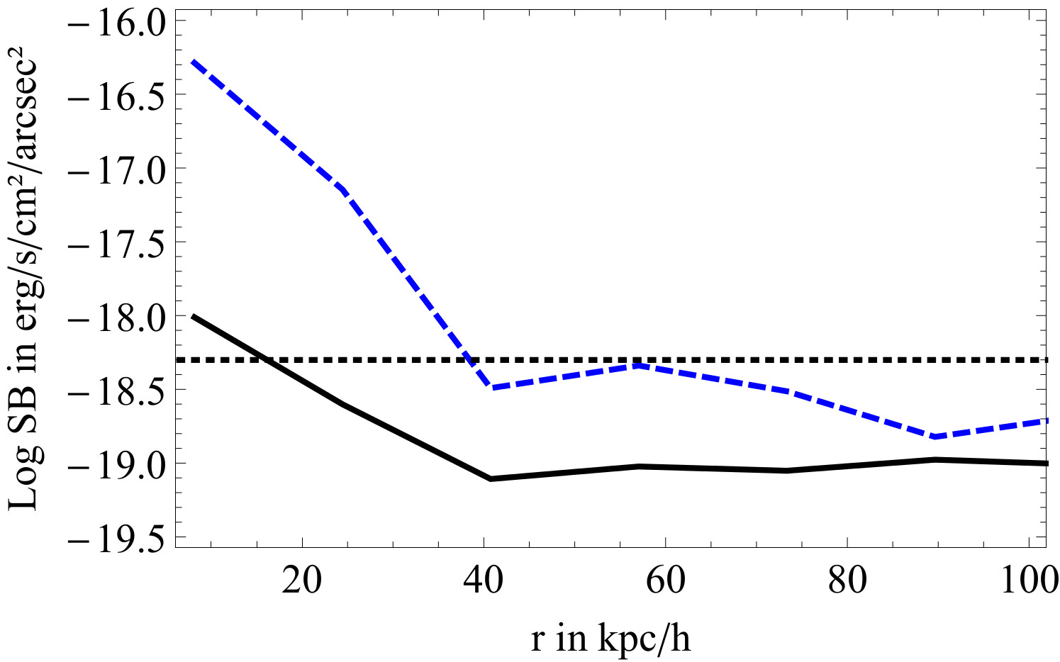
Figure 4: Surface brightness profiles for two sources with observed fraction of $\sim$ 30$\%$, with masses of 1.9 $\times$ $10^{10}$ $M_{\odot}$ (black solid line) and 7 $\times$ $10^{11}$ $M_{\odot}$ (blue dashed line). The horizontal dashed line indicates the detection threshold. On average, there were only 2 pixels per source above the detection threshold, and over 90% are detected in less than 5.5 pixels.(Comment: This plot was added.)

One can also obtain the luminosity function for our simulation, shown in fig. 3 for the three different lines of sight at redshift 4. We also show the intrinsic luminosity function (triangles) of our simulation. The overall shape of the luminosity function is not changed by the RT process. The drop at the low luminosity is due to incompleteness, since LAEs that are below the detection limit have an apparent luminosity of zero. The detection threshold and the assigned intrinsic luminosity introduce a free parameter in our model, shifting the luminosity function by a constant factor. Since we are mostly interested in changes of the observed fraction relative to the mean, we ignore this shift here.

4.2 Correlations between Large Scale Structure and Observed Fraction

In this section, we focus on our results from the redshift 4 snapshot.

Figure 5 shows how the observed fractions correlate with the dark matter overdensity $\delta$, the density gradient along the line of sight, the line of sight velocity and the line of sight velocity gradient, all evaluated at the positions of the sources for three different lines of sight. The observed fraction is given relative to the mean observed fraction,

$$\Delta\epsilon=\frac{\epsilon}{\bar{\epsilon}}\,\,.$$ (7)

The mean observed fraction $\bar{\epsilon}$ is 30/63/87% for our fiducial runs at redshift 4/3/2. ZCTM10 find a much lower mean observed fraction of a few percent at redshift 5.7. Laursen et al. (2011) also calculated observed fractions from nine simulated galaxies at 3.5. Although their sample is small, their mean observed fraction is around 24% (also note they do include photon destruction by dust).

We use the full sample of emitters and generate the plots of the correlations applying a moving average to the data set, averaging over 4000 emitters per data point. As described above, densities and (linear) velocities are obtained from the smoothed dark matter particle data. Density gradient, velocity and velocity gradient plots depend on the line of sight chosen, so we plot the relevant component $x_{i}$ or the derivative with respect to $x_{i}$, where $x_{i}=x,y,z$ for observers located along the respective axis.

The correlation between density and velocity gradient follows directly from the continuity equation (see eq. 3). Statistically, this also holds for the individual components of the divergence, i.e., the line of sight velocity gradient. The correlation between line of sight velocity and line of sight density gradient is quite intuitive: halos beyond a large scale overdensity move towards it and hence towards the observer, and vice versa. Both correlations are shown in fig. 10 and fig. 11. Because of this direct connection between the two pairs of observables, we discuss each of the pairs together.

As can be seen in fig. 5, correlations differ between different lines of sight. Although the trends are mutually consistent, deviations of up to 10% are clearly visible. We interpret this as a consequence of cosmic variance. Investigation indeed shows that the halo distribution and velocity fields clearly differ among different lines of sight, which can be expected for a box of this size. As an example, in fig. 9, the $x/y/z$-component of the halos’ velocity is plotted against the $x/y/z$-coordinate. For this plot, velocities are directly obtained from the dark matter particles, but the linear approximation we use to build the correlation plots shows the same behavior, i.e., a large scale, sine-like signal. This velocity distribution reflects the density structure in the box, as can be seen by comparison with fig. 9.

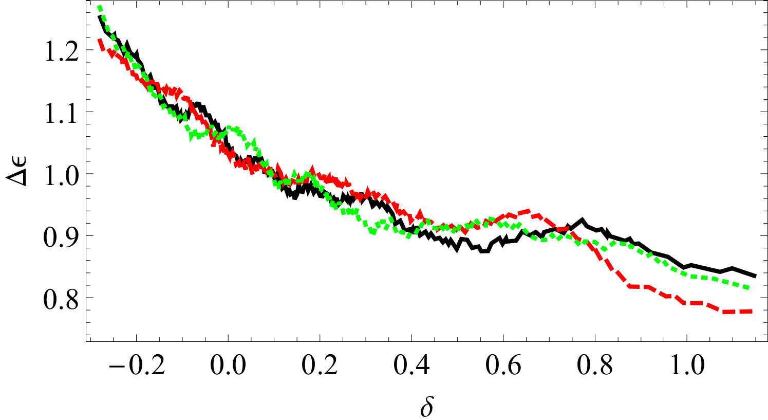
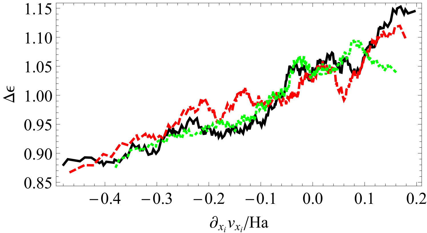
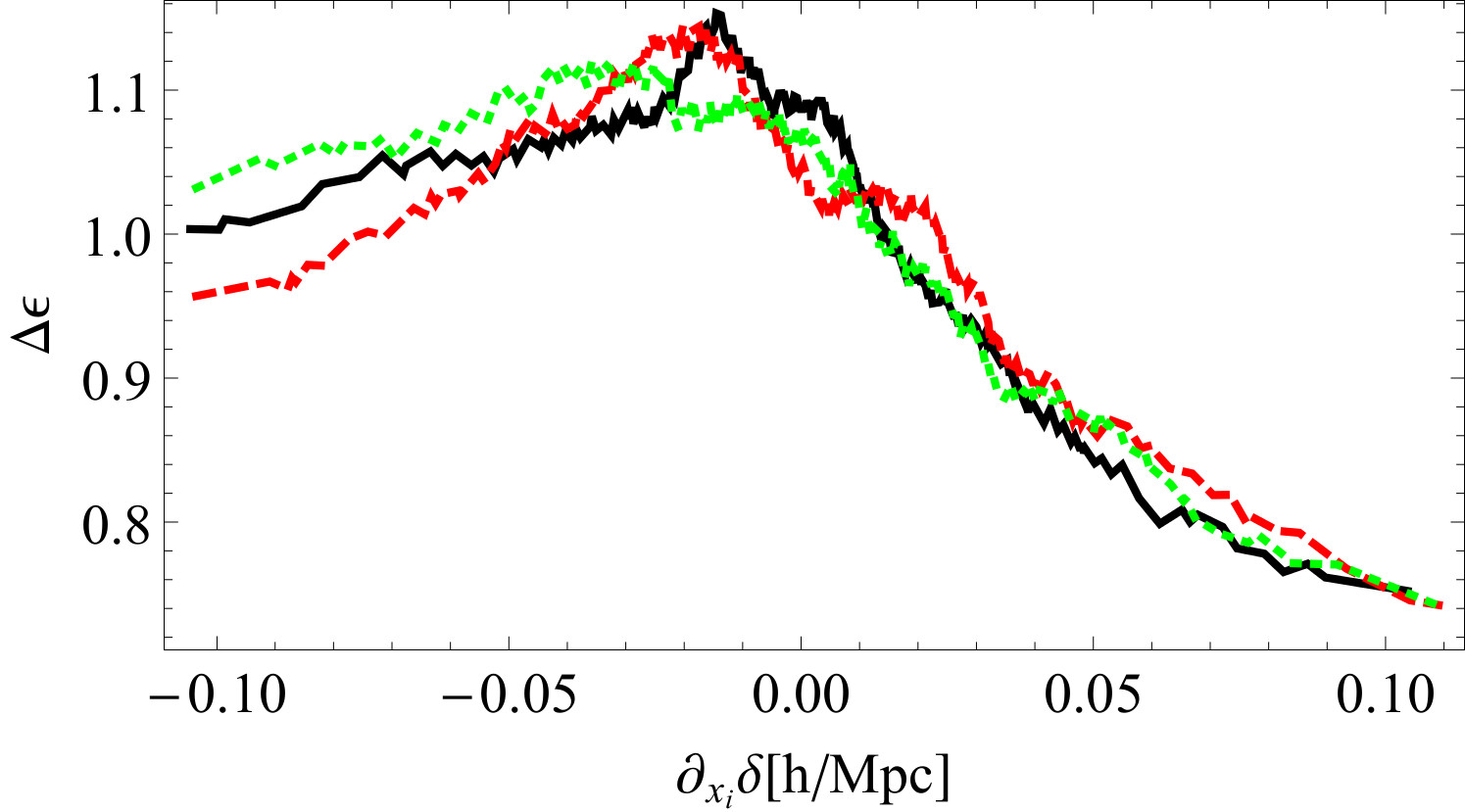
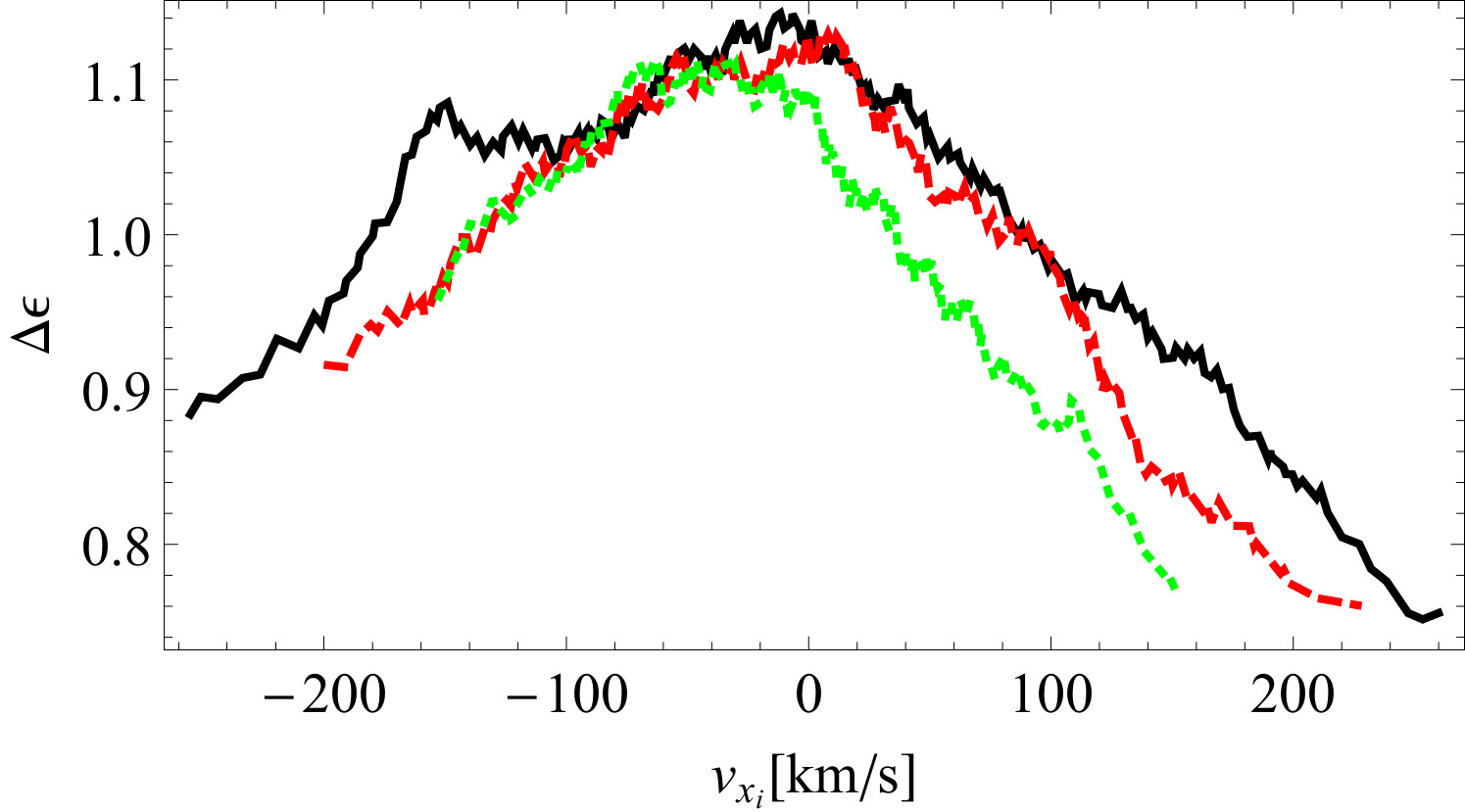
Figure 5: Correlations between observed fraction and large scale structure. On the $y$-axis, the relative observed fraction is shown in all four plots. The $x$-axis shows density (upper left), the line of sight velocity gradient (upper right), the line of sight density gradient (bottom left) and the line of sight velocity (bottom right). The three different lines correspond to the observer being located along the $x$-axis (black, solid), $y$-axis (red, dashed) and $z$-axis (green, dotted).

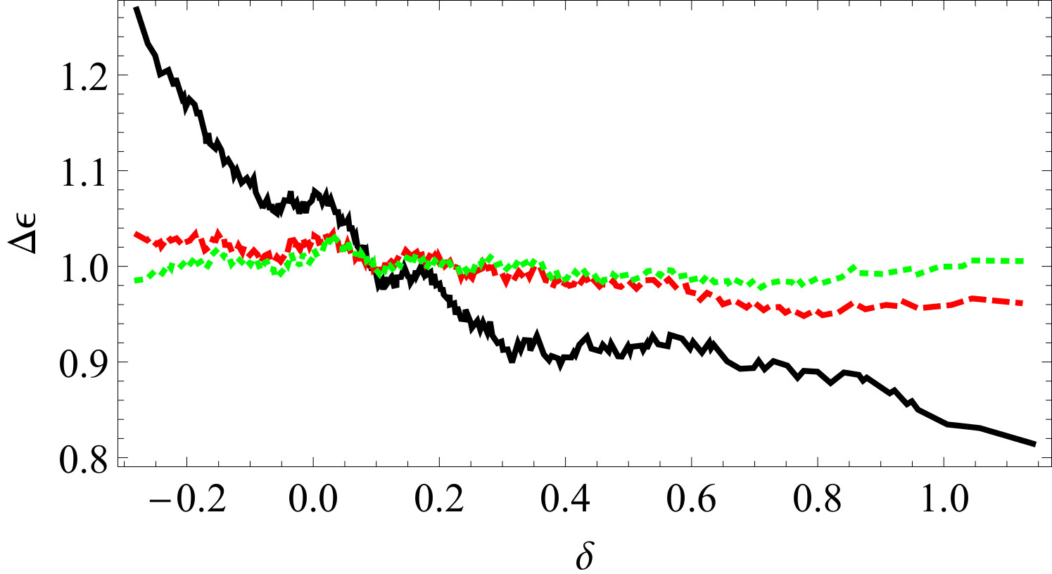
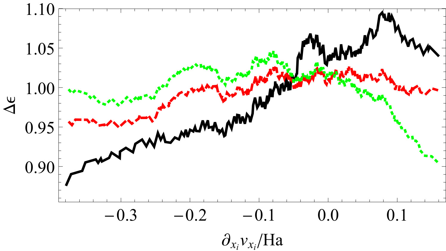
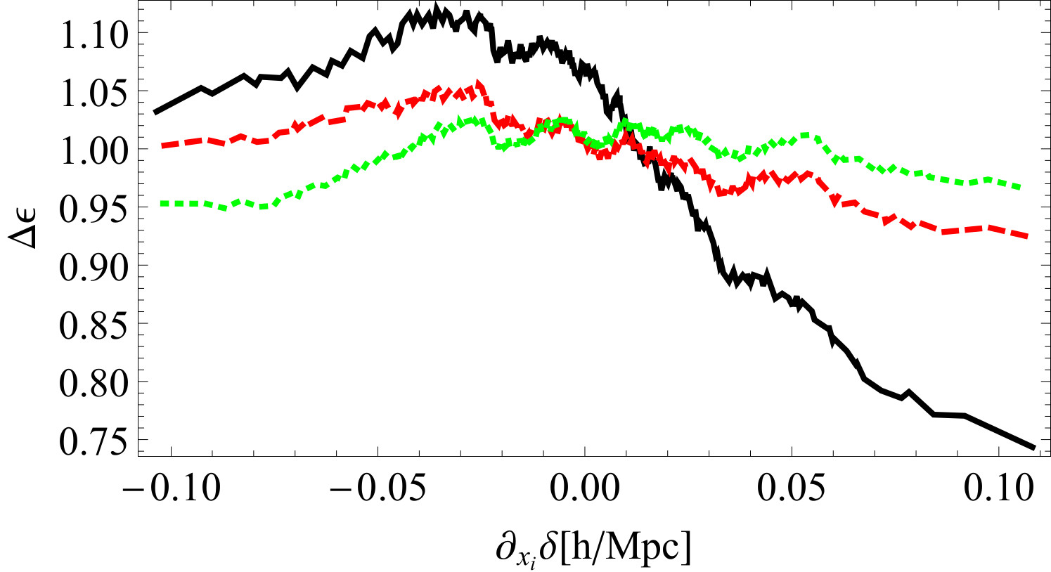
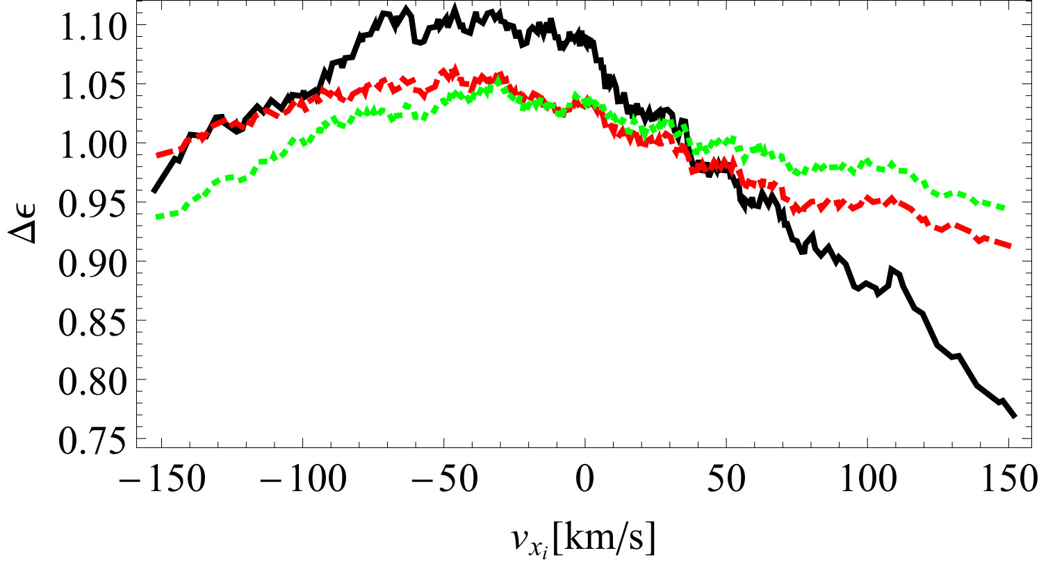
Figure 6: Same as fig. 5, but here the lines correspond to the fiducial case (black, solid), a run without peculiar motions and Hubble flow (red, dashed) and a simulation with peculiar velocities, but without Hubble flow (green, dotted), as seen by an observer along the $z$-axis.

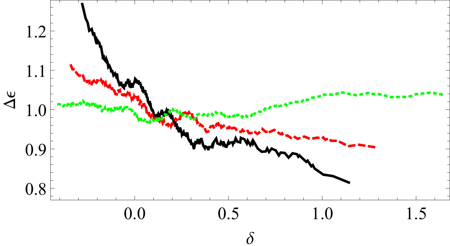
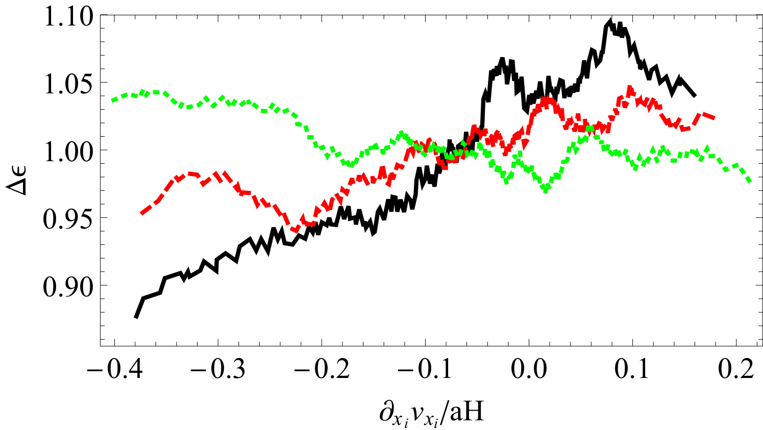
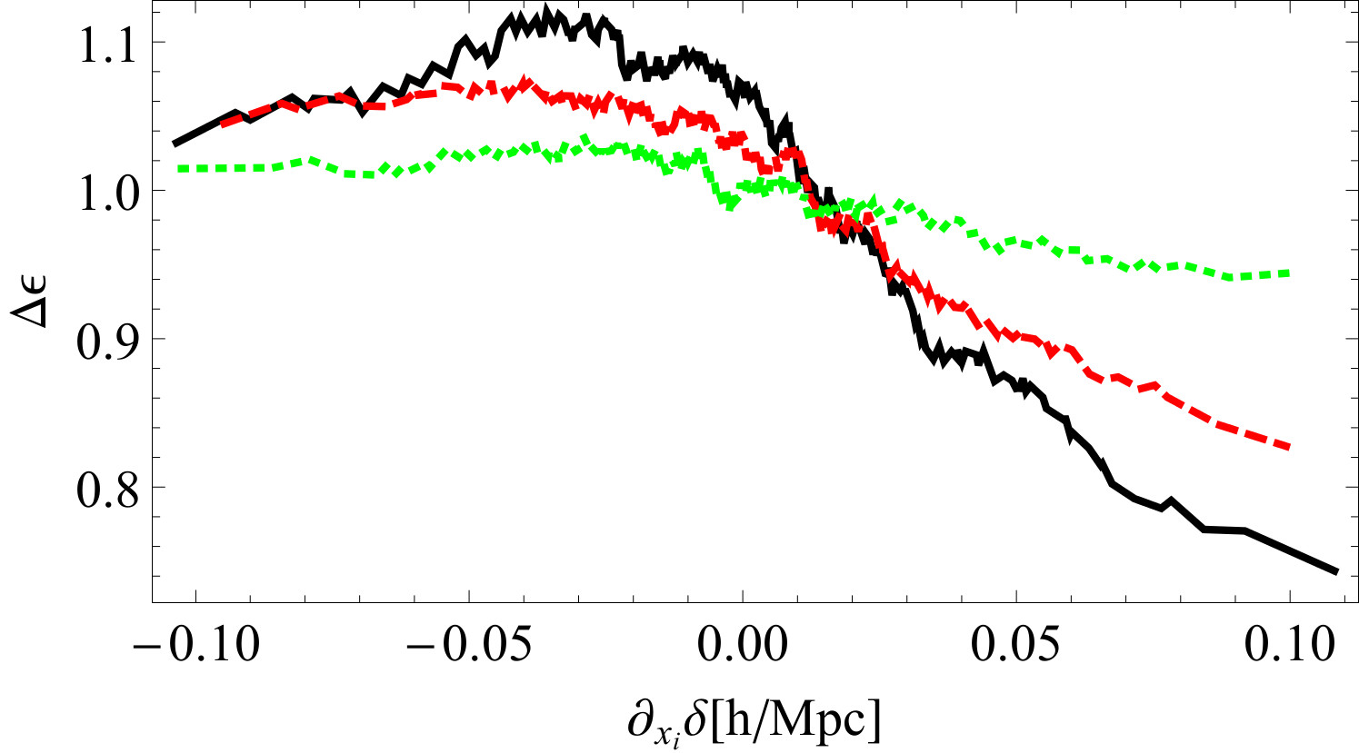
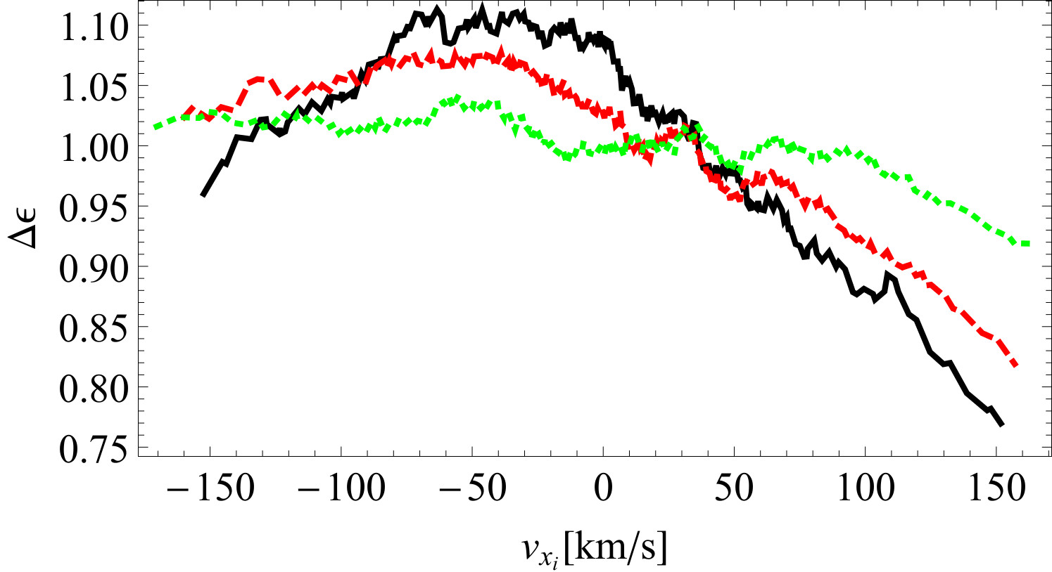
Figure 7: Same as fig. 5, showing the redshift dependence of the correlations. The data for a redshift of $z=4$ (black, solid), $z=3$ (red, dashed) and $z=2$ (green, dotted) is shown. The observer is located along the $z$-axis.

4.2.1 Density

As can be seen in the top left plot in fig. 5, larger overdensities are correlated with lower observed fractions. The effect is quite strong with about 30% in amplitude. We interpret this as a result of diffuse scattering around halos in overdense regions. Interestingly, the signal is highly suppressed if we switch off either the Hubble flow or the peculiar velocity field (see fig. 6, upper left subplot). Turning off the velocity field renders the spectra nearly symmetric. Photons that leave the ISM are not subject to further scattering, because neither local gas flows nor Hubble expansion can shift the photons back into the line center. This interpretation is also supported by calculations of the mean optical depth of the box. While in the line center, the optical depth (assuming a temperature of $2\times 10^{4}$ K and taking the mean HI density from the simulation volume) is still $\tau\sim 10^{2}$, a shift of 1 $\AA{}$ (in the local frame at $z=4$) reduces the optical depth to $\tau\sim 10^{-3}$. This also makes clear why velocity fields are so crucial in the radiative transfer.

When we turn on the peculiar velocity, the signal remains weak, but there is a slight decrease in observed fraction for halos in underdense regions. We interpret this as a result of the fact that in those underdense regions, small halos are dominant. The ISM in small halos doesn’t push the photons as far out into the wings as in the larger ones, so the probability of being scattered in the IGM is increased. Switching on the Hubble flow as well leads to our fiducial case: the Hubble flow together with the peculiar velocities leads to more numerous scatterings in overdense regions compared to the underdense regions.

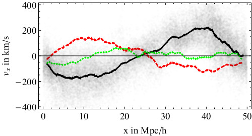
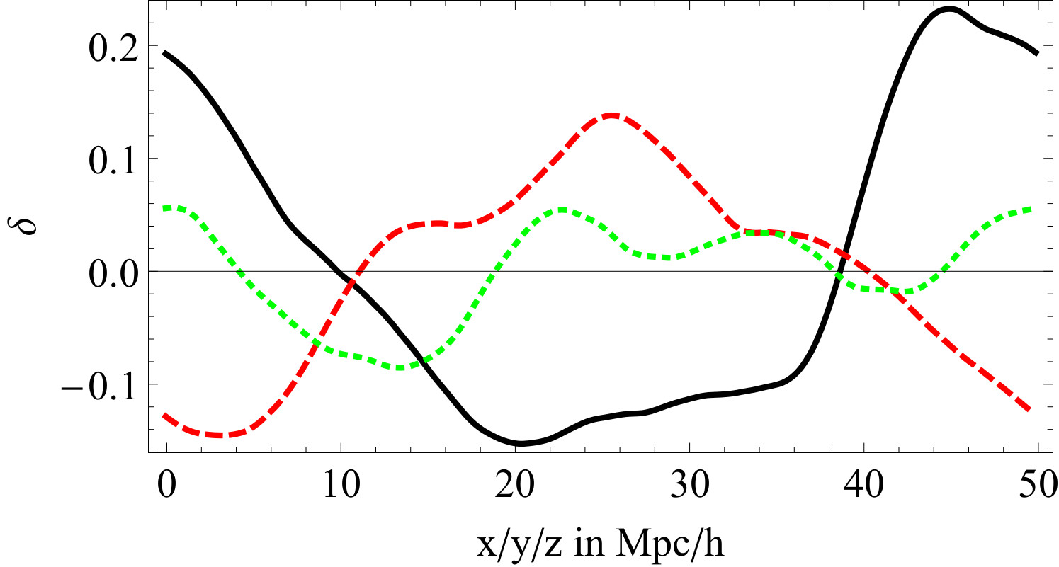
Figure 8: Averaged line of sight component of the halo velocities versus their location along the line of sight at $z=4$ for three lines of sight parallel to the $x$-/$y$-/$z$-axis (black solid/red dashed/green dotted).To illustrate the scatter, the distribution of halos is plotted in gray for the $x$-axis data.

Figure 9: Projected dark matter density along the $x$/$y$/$z$-axis (black solid, red dotted, green dashed line), smoothed on a scale of 10 Mpc/h for $z=4$.

4.2.2 Line of sight velocity gradient

The top right plot shows the correlation between line of sight velocity gradients and observed fractions. Here, we obtain qualitatively the same result as ZCTM10, although with a much lower amplitude; larger velocity gradients lead to a higher observed fraction. As has been discussed above, one can see that the effects of density and velocity gradient are anti-correlated as expected from linear theory (cf. fig. 11). For this reason, there is no meaningful way to completely disentangle the two physical mechanisms. However, the dominant effect from the velocity gradient can be understood from the fact that a higher velocity gradient corresponds to a higher local effective Hubble flow. Since most of the photons that leave a halo are blue, the higher the effective Hubble flow, the faster the photons are transported through the line center and into the red wing. If we turn off the Hubble flow, the effect is reversed: Now, a positive local gradient suppresses the emitters. This might be due to the fact that in this case, the redshifting through the line center takes place on a much larger length scale because the peculiar velocity gradient is much smaller than the Hubble flow.

It is worth pointing out that while in our simulations the amplitude of the correlation with line of sight velocity gradient is of the same order of magnitude as for the other correlations examined, ZCTM10 find a larger amplitude for the line of sight velocity gradient by about one order of magnitude. There are several factors that might be at play here. First of all, ZCTM10 worked at a higher redshift of $z=5.7$. The mean density is about 2.5 times higher at that redshift and therefore, the optical depth in the IGM is naturally higher, leading to more scatterings in the diffuse large scale environment. This might leave a stronger imprint of the bulk velocity fields (and their spatial evolution) in the observed fraction. Secondly, whereas ZCTM10 semi-analytically map the baryons onto the results of a pure $N$-body simulation, our gas distribution follows from a high-resolution hydrodynamical simulation that includes the effects of nonlinear in- and outflows which reduce the correlations with flows on linear scales. Additionally, we resolve the ISM at least marginally, leading to a large number of scatterings in the dense regions where the photons are emitted. After being processed through the ISM, the photons have already been shifted from the line center to some extent. This also leads to less scattering in the IGM, further reducing the impact of the large-scale velocity field on the observed fraction.

4.2.3 Line of sight density gradient

This correlation is shown in the bottom left plot of fig. 5. Due to the orientation of the observer towards the box, negative values here indicate that the density decreases in the direction of the observer. This makes the general trend in the plot plausible: observed fractions are lower if there is an intervening large scale overdensity region between the emitter and the observer. The effect becomes smaller when turning off Hubble flow and peculiar velocities, as can be seen in the lower left plot of fig. 6. This is probably due to the fact that the density of the environment becomes less important, as discussed in the preceding paragraphs. In contrast to ZCTM10, we find a prominent peak in the density gradient signal, at a value of around zero. We attribute this effect to the fact that halos with a density gradient of $\sim$ 0 are predominantly located inside lower density regions and voids. Due to the correlation of higher observed fractions with lower densities, those halos have a higher observed fraction. Analysis indeed shows that those low density halos ($\delta<0$) populate the region around $\partial_{x_{i}}\delta$ $\sim$ 0, and that their mean observed fraction is about 6% higher than the mean observed fraction of halos in denser regions. The mean density at the location of halos with a density gradient between -0.03 and 0.0 h/Mpc, for example, is reduced by a factor of 50% with respect to the full sample. Additionally, one can also notice that large absolute density gradients correspond to halos that are near to the large scale overdensity, and therefore in a region where the density is increased. For example, the mean large scale overdensity for halos with a density gradient $<-0.08$ h/Mpc is roughly twice the mean of the whole sample. Since this increases the optical depth also for the halos on the near side of the halo, it could also account for the dip on at large negative density gradients. This hypothesis is also supported by the fact that the effect does not fully vanish when the velocity field is set to zero, cf. fig. 6.

4.2.4 Line of sight velocity

In the bottom right plot, the correlation between line of sight velocities and observed fractions is shown. The box is orientated so that halos moving into the direction of the observer have positive velocities. The plot’s shape and the peak at around zero stays the same even if we turn off the peculiar velocities in the simulation, as can be seen in the lower right plot in fig. 6. This indicates that the correlation is dominated by the density gradient which looks nearly the same as the velocity signal when we turn off peculiar velocities. This is quite plausible since density gradient and velocity fields are highly correlated, cf. fig. 10. With Hubble flow and peculiar velocities switched on, we see a much larger amplitude and a strong suppression at positive velocities. Since halos with positive velocity are moving towards the observer while those with negative velocities are receding, we interpret this as a consequence of the Hubble flow that suppresses blue halos more strongly than the red ones.

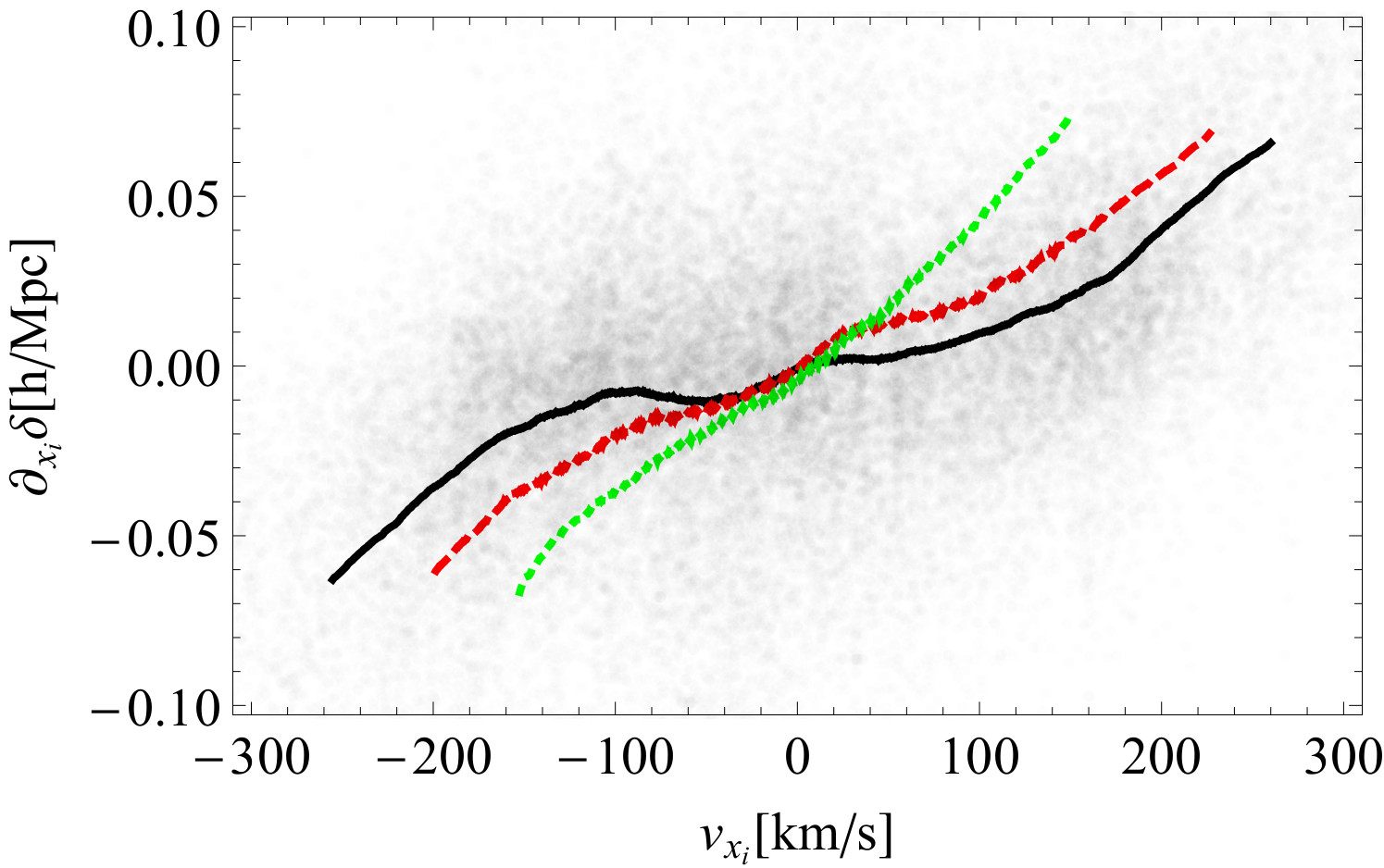
Figure 10: Here, we show the correlation between the line of sight density gradient and the line of sight velocity for all three lines of sight at $z=4$, x-axis (black, solid), y-axis (red, dashed) and z-axis (green, dotted). The gray dots show the scatter, each point representing one halo (for the x-axis data). See text for details.

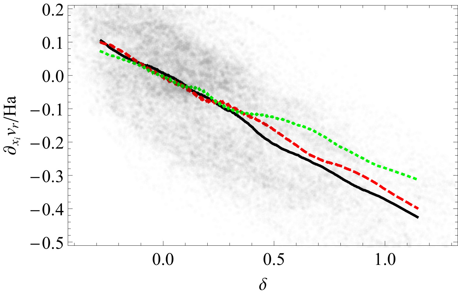
Figure 11: Correlation between the density and the line of sight velocity gradient for all three lines of sight at $z=4$, x-axis (black, solid), y-axis (red, dashed) and z-axis (green, dotted). The gray dots show the scatter, each point representing one halo (for the x-axis data). See text for details.

4.3 Evolution with Redshift

In fig. 7, the results for the dark matter correlation are shown for the redshift $z=2,3,4$. For this part of the analysis, the smoothing scale of the dark matter particles was adjusted to stay in the linear regime at lower redshifts. As has been discussed in a preceding section, the detection limit and the prescription of the intrinsic luminosity are somewhat arbitrary. Since the total mean density of the universe increases with redshift, we get different mean observed fractions at lower redshifts. At redshift 4, we have a total observed fraction of 30%, at redshift 2 it has risen to above 80%. For individual emitters, the observed fraction cannot be much larger than unity, so a higher total observed fraction can result in a compression of the correlation signal.

We find that correlations decline in amplitude with decreasing redshift. Since the mean density of the IGM decreases, the influence of the environment of the halos weakens. For the correlation of the observed fraction with the line of sight velocity, the drop of the Hubble rate from $\sim$ 400 km/s/Mpc at $z=4$ to $\sim$ 200 km/s/Mpc at $z=2$ further reduces the influence of the Hubble flow on the observed fractions from halos that move towards the observer ($v_{r}>0$).

While for the density gradient and the line of sight velocity, this decline in amplitude preserves the overall trend, for the density and the line of sight velocity gradient the lowest redshift $z=2$ shows a slight turnaround. For this redshift, halos in dense regions and in regions with a smaller velocity gradient are preferred by a few percent. One possible explanation is that a this later stage of structure formation, the medium in those dense regions is hotter and therefore contains less neutral gas. Since overdensities and low velocity gradients are coupled, this also affects the velocity gradient correlation.

In table 1, we show the results for linear fits to the general trends seen in the correlations. They were calculated ignoring the dip on the left side in the density gradient and velocity plots (i.e. the left edge of the velocity- and density gradient range). Due to the nonlinearity of the density correlation, the fitted value for this plot strongly depends on the chosen range for the fit. We obtained our fitted value by ignoring the steep decline below $\delta=0$.

Table 1: Evolution with redshift

	z=4	z=3	z=2
$\partial_{\delta}\Delta\epsilon$	-0.48	-0.15	-0.05
$\partial_{\partial_{r}\delta}\Delta\epsilon$	-3.0	-1.94	-0.78
$\partial_{v_{r}}\Delta\epsilon$	1.9 $\times 10^{-3}$	1.1 $\times 10^{-3}$	3.0 $\times 10^{-4}$
$\partial_{\partial_{r}v_{r}}\Delta\epsilon$	0.41	0.2	-0.08

4.4 Effects on the Two-Point Correlation Function

We calculate the two-point correlation function (2PCF) for our simulation data following Landy & Szalay (1993) using a standard estimator that is frequently written as:

$$\xi(r_{\perp},\pi)=\frac{DD-2DR+RR}{RR}\,\,,$$ (8)

where $DD$ is the pair count of galaxies in the simulations, $RR$ is the pair count of random positions drawn from a uniform distribution, and $DR$ is the count for pairs consisting of one random location and one galaxy, all separated by a distance $\pi$ along the line of sight and $r_{\perp}$ orthogonal to that.

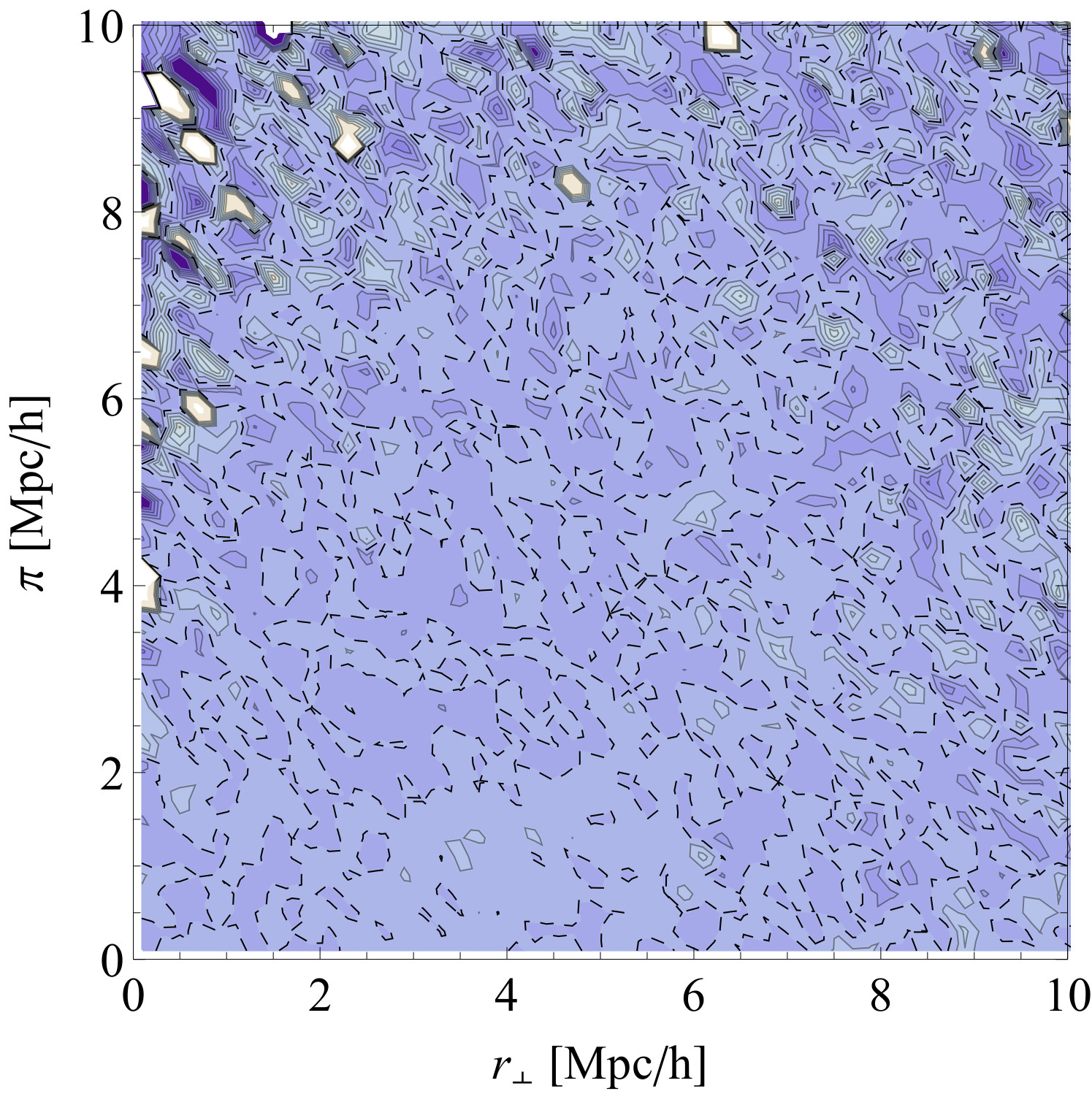
Figure 13: Ratio of the 2PCF of S-LAE and LAEs $\xi_{diff}=(\xi_{LAE}-\xi_{S-LAE})/\xi_{S-LAE}$. Contours are separated by 15%, the dashed contour corresponds to a value of 0. Number densities and thresholds are the same as in fig. 12.

The real space 3D-2PCF as a function of line of sight separation ($\pi$) and orthogonal separation ($r_{\perp}$) is shown in fig. 12 for halos (left), LAEs (middle) and a shuffled LAE sample (right)for our fiducial case with the Ly$\alpha$ detection limit set as explained above. The shuffled LAE sample was constructed following ZTCM11 by randomly shuffling the properties of the simulated LAEs to get rid off any correlation between apparent luminosity/observed fraction and the spatial location within the box. For all three samples, the number density was fixed to 4 $\times$ $10^{-2}$ Mpc^-3 h³ which corresponds to a (apparent) luminosity threshold of 0.6 $\times$ $10^{42}$ erg/s for the LAE/S-LAE sample and a mass threshold of 3.6 $\times$ $10^{10}$ $M_{\odot}$ for the halos. The redshift is $z=4$ for which we obtained the largest amplitude in correlations (see above). Near to an orthogonal separation of $\sim$ 0, the plot shows relatively strong fluctuations. Those are induced by the small sample size near $r_{\perp}\sim 0$ and by the finite resolution of our output grid, resulting in source blending; the projected distance of LAEs in this region is too small to disentangle them. We do not find a significant deformation of the 2PCF. ZCTM10 report an strong elongation pattern in the 2PCF along the line of sight direction which they attribute to a correlation between observed fraction and line of sight velocity gradient. In fig. 13, we plot the relative deviation of the LAEs’ 2PCF with respect to the shuffled sample, $\xi_{\rm diff}=(\xi_{\rm LAE}-\xi_{\rm S-LAE})/\xi_{\rm S-LAE}$. As can be seen, there is no indication of a deformation. We also tried different higher detection limits and luminosity thresholds, but didn’t find a significant elongation pattern. Also, the correlation with line of sight velocity gradient is not stronger with a higher detection threshold. We conclude that in contrast to ZCTM11, we do not find a significant elongation in the line of sight direction.

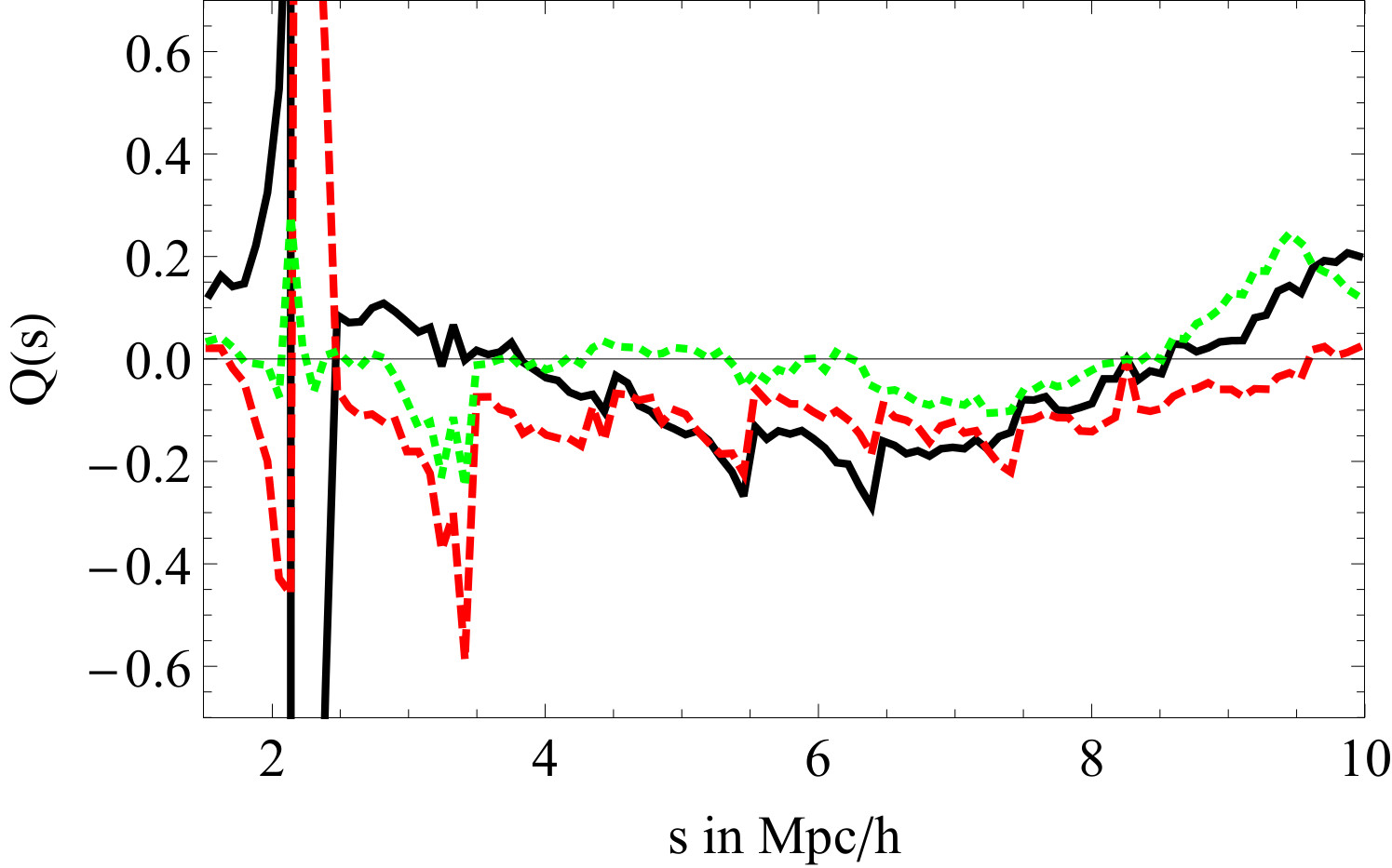
Figure 14: Q(s) for $z=4$ halo sample (black solid), LAE sample (red dashed) and S-LAE sample (green dotted line). Number density is 4 $\times$ $10^{-2}$. The spikes at 2-3 Mpc/h are due to poles.

In addition to the visual inspection of the 2PCF contours, we computed its quadrupole moment in order to quantitatively verify the absence of a distortion effect from Ly$\alpha$ RT. In fig. 14, we show the normalized quadrupole $Q(s)$ (e.g. Chuang & Wang (2012)) as defined by

$$Q(s)=\frac{\xi_{2}(s)}{\xi_{0}(s)-3/s^{3}\int_{0}^{s}\xi_{0}(s^{\prime})s^{\prime 2}ds^{\prime}}$$ (9)

where $\xi_{0}(s)$/$\xi_{2}(s)$ is the monopole/quadrupole contribution as a function of $s=\sqrt{\pi^{2}+r_{\perp}^{2}}$ .

Even for a threshold of $1\times 10^{-17}$ $\textrm{erg s}^{-1}\textrm{cm}^{-2}\textrm{arcsec}^{-2}$ which removes 90 % of all emitters, no significant signal was found in the magnitude of the quadrupole moment.

Again, this result can at least in part be attributed to our lower redshift. The amplitude of the selection effect induced by the RT and the observation threshold strongly depends on the optical depth in the IGM. The denser and more neutral IGM in ZCTM10/11 results in a stronger dimming of the central regions of a source, leading to a lower observed fraction. By tuning the observation threshold alone, this cannot be mimicked.

On the other hand, the linear analysis by Wyithe & Dijkstra (2011), evaluated with coefficients estimated from our results, indicates that our box size may be insufficient to measure a signal. Specifically, Wyithe & Dijkstra (2011) present an analytical model for estimating the impact of the radiative transfer on the clustering signal. The parameters $C_{v}$ and $C_{\rho}$ defined in their eq. 12 and 13 measure how the relative transmission of the IGM is affected by fluctuations in the velocity gradient and density field, respectively. These quantities are comparable by construction to $\partial_{\partial_{r}v_{r}}\Delta\epsilon$ and $\partial_{\delta}\Delta\epsilon$ used above.

We compare with our results in table 1 by computing $C_{v}$ and $C_{\rho}$ with values estimated from our data, namely the fraction of photons scattered in the IGM, $F\approx 0.7$, the mean IGM optical depth, $\tau_{IGM}\approx 1.5$, and the luminosity function power law index, $\beta=2.2$. We obtain $C_{v}\approx 0.6$ and $C_{\rho}\approx-1$ from the analytic model, which is broadly consistent with our values for $\partial_{\partial_{r}v_{r}}\Delta\epsilon$ and $\partial_{\delta}\Delta\epsilon$. At this level of $C_{v}$, the analysis of Wyithe & Dijkstra (2011) would suggest a small but noticeable deformation of the 2PCF. We consequently cannot rule out that the absence of a signal in our results is affected by our limited statistics.

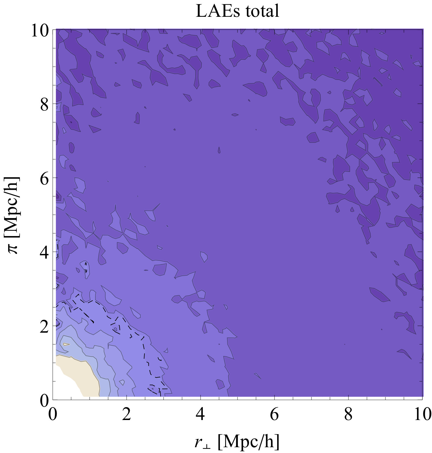
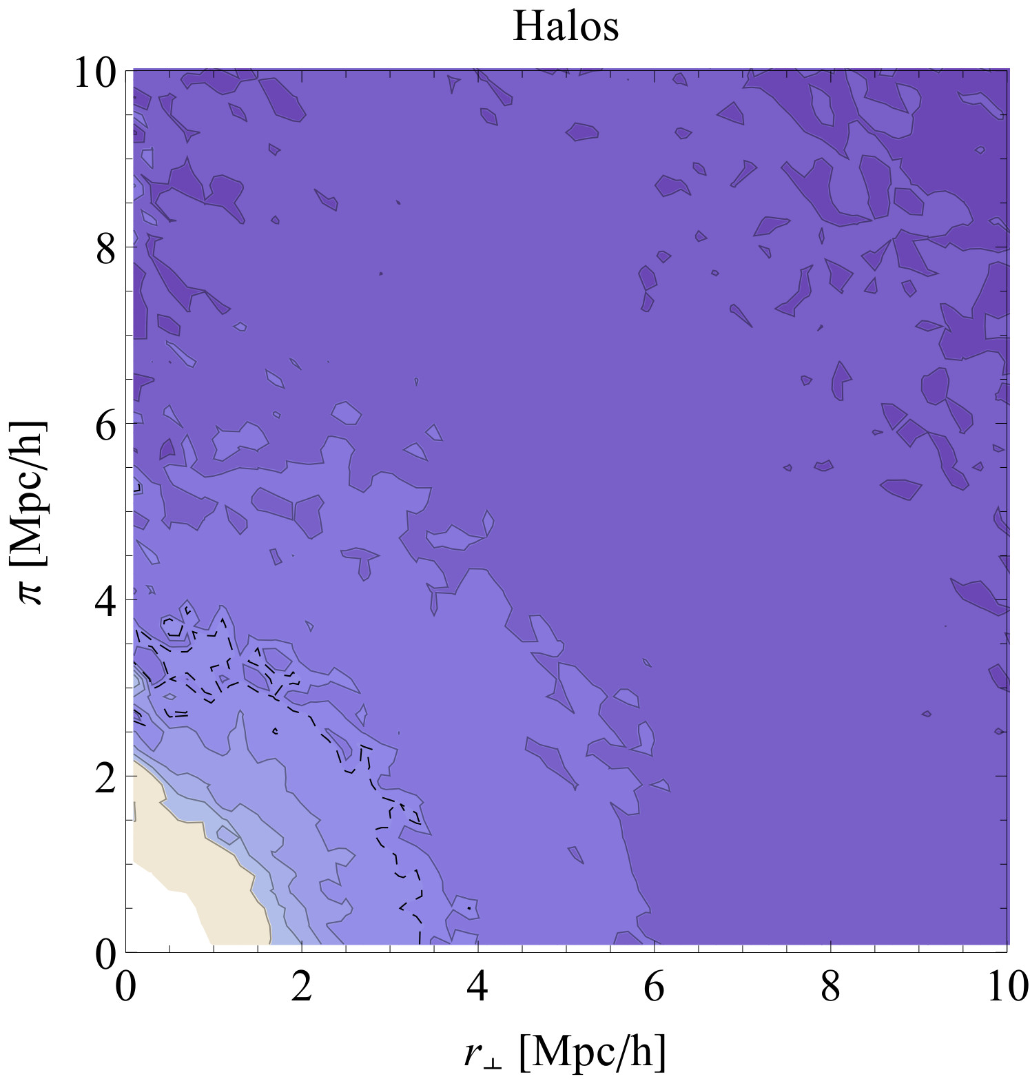
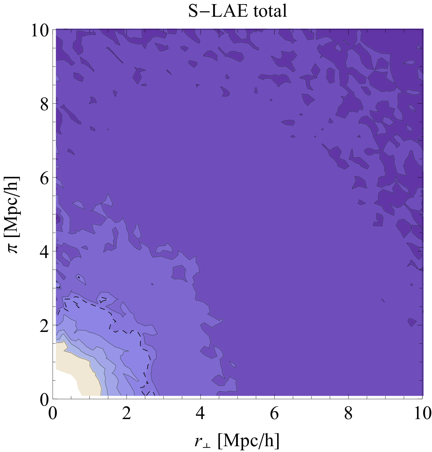
Figure 12: 2PCF as a function of line of sight ($\pi$) and perpendicular distance ($r_{\perp}$) for halos (left plot), observed LAEs (middle) and S-LAE sample (right) in real space at $z=4$. The dashed contours corresponds to $\xi=1$, contours are separated by 0.4. The number density of all threshold samples is 4 $\times$ $10^{-2}$ Mpc^-3 h³. The plots were averaged over three different lines of sight to reduce cosmic variance.

4.5 Impact of Inclination on the Observed Fraction

In fig. 15, the correlation between observed fraction and the inclination angle between the line-of-sight and the angular momentum of the dark matter halo is shown for all three redshifts. For this plot, we use the full sample of simulated LAEs. We use the dark matter angular momentum as a proxy for the disk orientation in order to avoid ambiguities in the definition of the disk plane, given the marginal resolution of galactic disks in the MareNostrum simulation.Of course, the scatter between disk orientation and halo angular momentum reduces the signal from disk orientation effects on the Ly$\alpha$ observed fraction as seen, for instance, in Bett (2012). On the other hand, this choice provides a more direct measure of the impact of halo tidal alignment on the clustering statistics, to be discussed below. For simplicity, we will refer to galaxies viewed along the direction of their halo angular momentum as “face-on”, in spite of the fact that the viewing direction may not be exactly normal to the disk plane.

For face-on galaxies, the observed fraction is increased by $\sim$15% with respect to edge-on galaxies. This is intuitive, since photons preferentially escape perpendicular to the disk because of the reduced optical depth compared to the path through the disk plane. Since this is local effect, it is independent of the chosen line of sight and is not affected by switching off/on the peculiar velocity field or the Hubble flow.

Strong inclination dependence has also been found by various groups (e.g. Laursen & Sommer-Larsen, 2007; Yajima et al., 2012; Verhamme et al., 2012) in simulations of isolated disk galaxies. Their results also showed a strong sensitivity on the morphology of the ISM, with a denser and clumpier structure exhibiting a significantly more pronounced dependence on viewing angle. In order to assess the full extent of LAE emission characteristics as a function of inclination angle, high-resolution simulations which provide a fair representation of the ISM morphology are required. Our results, based on a simulation with marginal spatial resolution of galaxies which results in a very smooth ISM structure, can therefore only provide a lower bound on the expected magnitude of the effect.

We do not find a significant evolution of the inclination dependence with redshift. This is surprising, since one might expect the disk-like shape to become more prominent at lower redshift due to the higher total mass in the ISM. Further investigation is needed to resolve this issue, but one has to keep in mind that comparisons of the signal’s amplitude can be difficult between different redshifts (cf. Sec. 4.3).

The signature of orientation dependence and tidal alignment on redshift space distortions (RSD) has been analyzed by Hirata (2009) who concludes that the effect is degenerate with gravitationally induced RSD (i.e., the Kaiser effect, Kaiser 1987) and may amount to several percent for reasonable assumptions about alignment and inclination dependence of the observed flux. However, it is easy to see that the coefficient that measures the orientation dependence (named $\psi$ in Hirata (2009)) can be made much larger if one assumes a very steep transition from edge-on to face-on flux, such as the one observed by Verhamme et al. (2012) in their case “G2”. The fact that the transition seen in our results (fig. 15) is rather smooth can be attributed to two effects that have already been mentioned above: first, the spread of disk orientations with respect to halo angular momentum washes out the overall signal, and second, the spatial resolution is inadequate to capture the full extent of the expected orientation dependence. While the former is physical and will be present in real data, the latter is an artifact of our method.

These results are highly suggestive that LAEs can provide a sensitive probe of gravitationally induced tidal alignment. This could reduce the accuracy of growth factor measurements from surveys like HETDEX; however, additional information from the galaxy bispectrum can break the degeneracy (cf. Krause & Hirata 2011). But it also offers the attractive opportunity to search for tidal alignment in LAE survey data and to test the predictions of CDM structure formation. For instance, recent results from large N-body simulations show an alignment along large-scale structure filaments for lower-mass halos, whereas the angular momenta of high-mass halos preferentially align perpendicular to the direction of filaments (Codis et al., 2012). Further work is needed to explore the potential of LAEs as tracers of cosmic alignment.

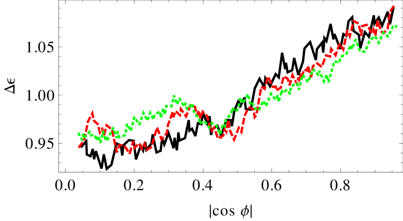
Figure 15: Correlation between the relative observed fraction and the inclination of the halos with respect to the observer. An inclination of 1 corresponds to a face-on emitter, 0 corresponds to edge-on. The lines show data from $z=4$ (black), $z=3$ (red) and $z=2$ (green)

5 Conclusions

Our numerical analysis clearly shows that resonant scattering in the CGM and IGM can strongly suppress observed Ly$\alpha$ fluxes. We find mean observed fractions between 30% at $z=4$ and around 80% at $z=2$. We stress that we do not include destruction by dust, hence the suppression in flux purely results from anisotropic escape of photons from their halos and diffuse scattering in the IGM. These results are consistent with Laursen et al. (2011).

We do find correlations between the large-scale density and velocity fields and the observed Ly$\alpha$ fraction. This broadly confirms the results of ZCTM10 who report a much stronger effect at higher redshifts. Apart from their overall smaller amplitude, the correlations seen in our work differ from those found by ZCTM10 in their relative strength. Whereas the velocity gradient has by far the strongest effect in their results, in our case it is comparable in magnitude to the correlations of Ly$\alpha$ observed fraction with large-scale density, density gradient, and velocity fields. This appears more natural to us since density and velocity gradient are correlated via the continuity equation.

All of the correlations with large-scale fields that we found have plausible interpretations in terms of resonant scattering with neutral hydrogen modulated by density and Doppler shift. Owing to the strong correlations between the density and velocity fields in the linear regime, it is not always possible to unambiguously identify the dominant effect. By artificially turning off the peculiar velocity and Hubble flow terms in the scattering cross sections, we were able to separate the effects of density and velocity to some extent. The results are consistent with intuitive expectations: the effect of large-scale overdensity is largest and similar to the velocity gradient, followed closely by velocity and density gradient.

For all correlations except orientation dependence, we find a strong decrease of their amplitude from redshift 4 to 2. Despite the strong impact of the radiation transport on the observed fluxes, we do not reproduce the clustering signal found by ZCTM11. Even at $z=4$ where the correlations are strongest, we fail to detect a significant change in the 3D 2PCF.

Although the lower redshift of our studies is expected to reduce the clustering signal, a comparison with the analytical model by Wyithe & Dijkstra (2011) suggests that this is not the full explanation. The values we find for the dependence of the observed flux on the large-scale velocity gradient would, according to their model, lead to a small but detectable deformation in the 2PCF. It is therefore plausible that the limited statistics due to our finite box size are partly responsible for our failure to detect non-gravitational clustering from Ly$\alpha$ RT effects.

We also found a distinctive correlation between the Ly$\alpha$ observed fraction and the angular momentum of the dark matter halo, which we interpret as a signal of the orientation dependence of LAE fluxes. Although the amplitude of the signal is only $\sim$ 15 % in our numerical analysis, we assume that it can be substantially larger in reality as our results are limited by poor spatial resolution of the ISM. In this case, partial alignment of halo spins with the large-scale tidal field may give rise to contaminating contributions to redshift space distortions (Hirata, 2009; Krause & Hirata, 2011). On the other hand, our results combined with recent high-resolution simulations of LAEs (Verhamme et al., 2012) suggest that LAEs provide a sensitive observational probe of tidal alignment.

Appendix A The physics of Ly$\alpha$ transport

A.1 General

Ly$\alpha$ photons emitted in starforming regions of a galaxy undergo resonant scatterings that result in a stochastic movement in space and frequency. As in many previous studies, we denote the frequency of a Ly$\alpha$ photon with the dimensionless quantity

$$x=\frac{\nu-\nu_{0}}{\nu_{D}}$$ (10)

where $\nu_{D}$ is the Doppler frequency, $\nu_{D}=\frac{v_{th}\nu_{0}}{c}$ with the most probable thermal velocity of the atoms $v_{th}=\left(\frac{2k_{B}T}{m_{H}}\right)^{1/2}$ and all other symbols having their usual meaning.

A non-zero bulk velocity of the gas $\@vec{v}$ can be taken into account easily by performing a first-order Lorentz transformation into the restframe of the macroscopic gas motion:

$$x^{\prime}=x-\frac{\@vec{v}\cdot\@vec{n}}{v_{th}}$$ (11)

Following Dijkstra et al. (2006), we denote quantities measured in the restframe of macroscopic bulk velocity with a prime. If not mentioned otherwise, quantities are measured in the frame of an observer which is at rest with respect to the center of mass (but notice the remarks on the Hubble flow in section B). Here, $\@vec{n}$ is the direction of the photon.

A.2 Absorption and Reemission

The scattering cross section of a Ly$\alpha$ photon can be written as

$$\sigma_{L}=f_{12}\frac{\sqrt{\pi}e^{2}}{m_{e}c\nu_{D}}H(a,x^{\prime})$$ (12)

with $f_{12}$ the Einstein coefficient and $H(a,x^{\prime})$ the Voigt profile that depends on the dampening parameter $a=\frac{\Delta\nu}{2\nu_{D}}$. $\Delta\nu$ is the natural line width.

Therefore, the optical depth $\tau$ for Ly$\alpha$ traveling a distance $l$ with frequency $x$ through a gas with neutral hydrogen number density $n_{H}$ is

$$\tau=\int_{0}^{l}\sigma_{L}\;n_{H}dl^{\prime}$$ (13)

The probability $P$ of a photon to pass through an optical depth $\tau$ without being absorbed is equal to

$$P=e^{-\tau}$$ (14)

Neutral hydrogen atoms on which the scatterings occur follow a specific velocity distribution due to their random thermal velocity and the macroscopic gas velocity, since photons are red/blueshifted in the frame of the scattering atom. It is convenient to split the thermal velocity into components parallel and orthogonal to an incoming photon. The PDF of the parallel component is

$$P(v_{z})=\frac{ae^{-v_{z}^{2}}}{\pi[(x^{\prime}-u_{z})^{2}+a^{2}]}H^{-1}$$ (15)

The other two components orthogonal to the direction of the infalling photon follow a Gaussian distribution.

Absorption is quickly followed ($\Delta t\sim 10^{-9}$ s) by reemission. The frequency of the reemitted photon depends on the scattering atom’s velocity due to the fact that the scattering is coherent in the atom’s restframe, but not necessarily in the reference frame of an observer. If $\@vec{v}_{a}$ denotes the atom’s velocity in the frame of the observer, then the relation between the frequency of the infalling photon $x_{i}$ and the reemitted photon $x_{r}$ satisfies

$$x_{r}=x_{i}+\frac{\@vec{v}_{a}\cdot(\@vec{n}_{r}-\@vec{n}_{i})}{v_{th}}$$ (16)

Where $\@vec{n}_{i}$/$\@vec{n}_{r}$ is a unit vector in the direction of the infalling/reemitted photon. We neglect the recoil on the scattering atom here, because it has been shown to have no significant effect on the radiation transport (Zheng & Miralda-Escude 2002). The distribution of the remission’s direction is determined by a phase function. Depending on the frequency of the infalling photon, different phase functions have been proposed for the angular distribution of Ly$\alpha$ photons. As shown in Tasitsiomi (2006), for numerical simulations the differences between the phase function are quickly washed out by the resonant scatterings. For that reason, we use an isotropic phase function that can be written as

$$P(\@vec{n}_{r}|\@vec{n}_{i})=\textrm{const.}$$ (17)

Since the frequency of the photons generally changes due to the scatterings, the photons perform a random walk in space and frequency (Harrington 1974). The cross section quickly decreases when a photon leaves the line center, so the mean free path will increase drastically for photon left/right of the line center. Typically, photons leave an optical thick medium after a couple of scatterings on atoms to which they appear strongly red- or blueshifted, because in that case, it is probable that the photon is reemitted with a frequency far away from the line center, measured in the reference frame of the observer.

Appendix B LyS - A Ly$\alpha$ Simulation Code

LyS is our implementation of a Monte-Carlo code for Ly$\alpha$ radiation transport. It is capable of tracking photons in grids with Adaptive Mesh Refinement (AMR). LyS is OpenMP-parallelized, so on machines with multiple cores, each core can handle one photon at a time. Additionally, MPI was implemented to deal with the large data set of the MareNostrum Galaxy Formation Simulation.

Similar to other codes, LyS solves the radiation transfer problem for individual photons via the following iterative algorithm:

1. Draw an optical depth $\tau_{0}$ exponentially distributed (eq 14)

2. Integrate the optical depth $\tau$ while the photon traverses a grid of gas cells (eq 13)

3. When $\tau$ equals $\tau_{0}$, a scattering point is reached. Draw the velocity of the scattering atom from the PDF in eq. 15

4. Calculate the new frequency and direction of the scattered photon according to eq. 16 and 17

The iteration is stopped when a photon has traveled a quarter of the box length from its source. If it it reaches a box boundary before, we apply periodic boundaries.

For the generation of the output, we use the so-called next event estimator or peeling-off method (Whitney 2011). At each scattering, we calculate the probability that the photon is reemitted into the direction of the observer and reaches the boundary of the box without further scatterings. This might be thought as sending out a ’tracer photon’ at each scattering event. The probability of reaching the observer is given by eq. 14, where $\tau$ is now the optical depth along the line of sight from the scattering point to the boundary of the box. Since the frequency of the reemitted photon depends on the direction into which it is emitted, one has to assign the frequency for the tracer photon according to eq. 16. The calculated probability is summed in the output array for each scattering. Assuming the observer is located in the direction of the positive x-axis, the array holds $n_{y}\times n_{z}\times n_{\lambda}$ bins for the y-/z-coordinate of the photon and the physical wavelength.

The line of sight integration used in the peeling-off method also applies periodic boundaries if the integration distance is less than a quarter of the box length (and stops the integration if this value is reached). This removes edge effects due to the finite extent of the box. One could also just skip sources near to the boundaries, but this would result in the loss of many emitters, degrading the statistics. Physically, this corresponds to a flattening of the volume in the line of sight direction. This is plausible since the box is thin relative to the distance to the observer.

During the line-of-sight integration, tracer photons are redshifted according to the linear Hubble Law.

Regular photons are also redshifted on their path through the volume. This is implemented by adding a term

$$\@vec{v}_{H}=-H\@vec{d}_{lsp}$$ (18)

to the bulk velocity in eq. 11, where $\@vec{d}_{scat}$ denotes the distance vector to the last scattering location of the photon and $H$ is the Hubble rate at the specific redshift. In this sense, each photon has its own frame of reference, in rest with respect to the observer’s frame, but seeing a spherical velocity field centered on the last scattering location.

To find random numbers following the distribution in eq. 15, we use the so-called rejection method (Press et al. 2007) in an implementation similar to Laursen et al. (2009a). LyS uses the acceleration scheme proposed by Ahn et al. (2002) which reduces the number of scatterings by skipping so-called core scatterings. This is done by cutting off the velocity distribution of the scattering atoms below some value, which effectively forces photons to be scattered by atoms to which they appear far in the blue or red. If the frequency $|x|$ is below a critical frequency $x_{cw}$, the components of the scatterings atom’s velocity that are perpendicular to the photon direction of flight are drawn via

$$v_{\perp,0}=\sqrt{x^{2}_{cw}-\log R_{4}}\cos(2\pi R_{5})$$ (19)

$$v_{\perp,1}=\sqrt{x^{2}_{cw}-\log R_{4}}\sin(2\pi R_{5})$$ (20)

Here, the $R_{i}$ are random numbers drawn from a uniform distribution.

In this paper, we focus on Ly$\alpha$ radiation from star forming regions near the center of young galaxies. Taking into account the resolution of our simulation box, it is a good approximation to emit photons at the center of the halos. Following ZCTM10, we choose the intrinsic Ly$\alpha$ luminosity of a halo proportional to its star formation rate $R_{SF}$, which is in turn a linear function of the halo mass $M_{h}$:

$$L_{i}=10^{42}R_{SF}\frac{\textrm{erg}\textrm{s}^{-1}}{\textrm{yr}^{-1}M_{\odot}}$$ (21)

$$R_{SF}=0.68\frac{M_{h}}{10^{10}M_{\odot}}\textrm{yr}^{-1}$$ (22)

Both equations should vary with redshift. The cosmic star formation history reached its peak around redshift 2 (Kobayashi et al. 2013), and the intrinsic Ly$\alpha$ luminosity should be modified by dust attenuation that is also a function of star formation history. We ignore this here, since from the perspective of our numerical simulation, the total intrinsic luminosity plays only the role of a normalization, especially because we are mostly interested in ratios between intrinsic and apparent luminosities. We also stress that we chose this specific model to be comparable to previous work, not because it is the relation predicted by the MareNostrum simulation. Photons are emitted with a frequency drawn from a Gaussian. Its width is determined by the viral temperature of the halo:

$$T_{vir}=\frac{GM_{h}\mu m_{H}}{3k_{B}c}$$ (23)

Here, $R_{vir}$ denotes the virial radius of the halo and $\mu$ is the mean molecular weight. In this way, we include the velocity distribution of emitters that are gravitationally bound. Photons are emitted from halos with mass $\geq$ 5 $\times$ $10^{9}M_{\odot}$. Since the range of masses and thus intrinsic luminosities is about 3 orders of magnitude, we follow ZCTM10 in applying a weighting procedure for the individual photons to reduce the total number of photons to compute. Each halo emits independently of its mass at least $n_{min}=1000$ photons. In total, we run the RT for about 40.000/49.000/51.000 halos at redshift 4/3/2. To conserve the relative intrinsic luminosities, photons are given a mass-dependent weight.

B.1 Code Verification

To verify the correctness of our radiative transfer code, we perform the standard tests from the literature. In figure 16, the redistribution function $f(x,x^{\prime})$ is shown, namely the probability for an infalling photon with frequency $x$ to be reemitted with a frequency $x^{\prime}$. In this test, only thermal motions of the scattering atom are considered. Overplotted are the analytical solutions by Lee (1974).

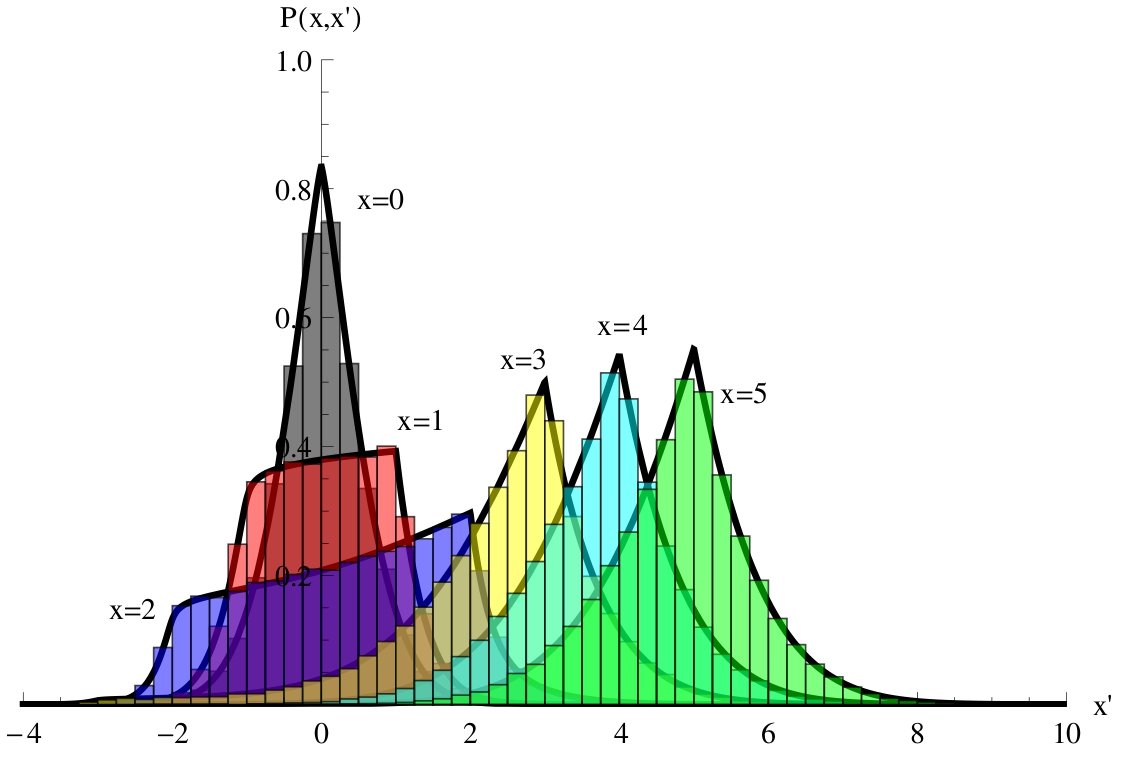
Figure 16: Comparison of the redistribution function calculated using the analytic solution by Lee (1974) (solid lines) with our code. Shown is the probability that a photon is reemitted with a frequency $x^{\prime}$ when it had the frequency $x$ before the scattering occurred for some values of $x$.

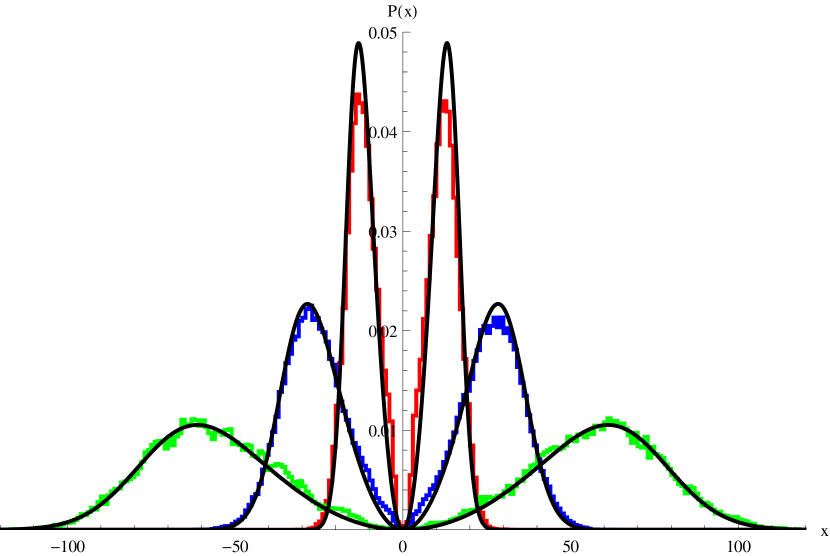
Figure 17: Comparison between the analytical solution (solid lines) of the spherical test case (see text) and the results as obtained by LyS. Shown is the probability distribution of the escaping photons as a function of the dimensionless frequency $x$. The innermost peaks correspond to an optical depth of $10^{5}$, the outermost to $10^{7}$. The third case is for an optical depth of $10^{6}$.

The standard test for Ly$\alpha$ -Codes, the so-called static sphere test, is shown in fig. 17 for various optical depths ($\tau_{0}=10^{5}/10^{6}/10^{7}$). In this test, photons are launched in the center an isothermal sphere of constant density. Overplotted is the analytic solution from Dijkstra et al. (2006). For these tests, the acceleration scheme was turned off. The static sphere test was also done with the activated acceleration scheme. It still resembles the analytical solution quite well.

For figure 19 and 18, the static sphere problem was modified with a Hubble-like bulk velocity field. The gas was assigned a velocity

$$\@vec{v}_{bulk}=\frac{v_{max}\@vec{r}}{r_{max}}$$ (24)

With some constant maximum velocity $v_{max}$, $\@vec{r}$ the distance vector from the center of the sphere and $r_{max}$ the distance from the center where $|\@vec{v}|=v_{max}$. Since there is no analytic solution for this test case available, we can only compare with other the results from other codes. The results from LyS are in good agreement with the plots in Faucher-Giguere et al. (2010) and Dijkstra et al. (2006).

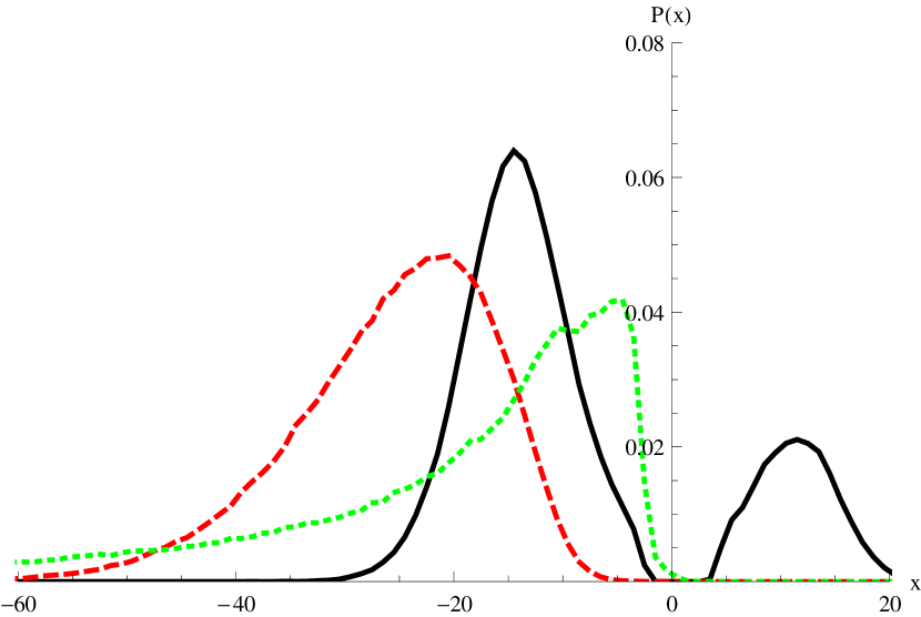
Figure 19: Same as figure 18, but for an expanding sphere. The different lines correspond to the maximum expansion velocities: 20 km/s (line), 200 km/s (dashed), 2000 km/s (dotted).