Self-Force and Green Function in Schwarzschild spacetime via Quasinormal Modes and Branch Cut

Abstract

The motion of a small compact object in a curved background spacetime deviates from a geodesic due to the action of its own field, giving rise to a self-force. This self-force may be calculated by integrating the Green function for the wave equation over the past worldline of the small object. We compute the self-force in this way for the case of a scalar charge in Schwarzschild spacetime, making use of the semi-analytic method of matched Green function expansions. Inside a local neighbourhood of the compact object, this method uses the Hadamard form for the Green function in order to render regularization trivial. Outside this local neighbourhood, we calculate the Green function using a spectral decomposition into poles (quasinormal modes) and a branch cut integral in the complex-frequency plane. We show that both expansions overlap in a sufficiently large matching region for an accurate calculation of the self-force to be possible. The scalar case studied here is a useful and illustrative toy-model for the gravitational case, which serves to model astrophysical binary systems in the extreme mass-ratio limit.

I Introduction

The motion of a point particle in curved spacetime can be modelled as the particle deviating from a geodesic of the background spacetime due to the action of its own field, which gives rise to the self-force (see Poisson:2011nh; Barack:2009ux for reviews). The particle may be a scalar charge, an electric charge or a point mass. In the case of an electric charge moving in flat spacetime, the self-force is the celebrated Abraham-Lorentz-Dirac force Dirac:1938nz. The case of a point mass serves to model, for example, a small compact object moving in the background of a massive black hole, i.e., an Extreme Mass-Ratio Inspiral. Such a binary system is of major astrophysical importance due to the expected ubiquity of massive black holes in our Universe Magorrian:1997hw.

Astrophysical black holes are expected to be rotating and as such their gravitational field is described by the Kerr metric. However, even in the simpler case of the static and spherically-symmetric Schwarzschild black hole background, the calculation of the self-force (SF) is technically challenging. This is partly due to the fact that the field of the small object diverges towards the position of the object itself and so regularization procedures are required. Various methods for the calculation of the SF are already in place and have been used by different research groups to achieve landmark results in the Schwarzschild background spacetime in the recent years. Among them, there is concordance between gravitational SF, post-Newtonian and Numerical Relativity calculations Blanchet:2009sd; LeTiec:2011bk, a gravitational SF correction to the frequency of the Innermost Stable Circular Orbit Barack:2009ey, a correction to the precession effect Barack:2010ny, evolution of a ‘geodesic’ SF orbit (i.e., where the motion is evolved using the value of the SF corresponding to an instantaneously tangent geodesic) in the gravitational case Warburton:2011fk and evolution of a self-consistent orbit (i.e., where the coupled system of equations for the motion and for the SF are simultaneously evolved) in the scalar case Diener:2011cc.

These results were obtained via two leading methods for SF calculations: the mode-sum regularization scheme Barack:2001gx; Barack:1999wf, and the effective source method Barack:2007jh; Vega:2007mc. Despite first appearances, these approaches share a common foundation: the SF is related to the gradient of a regularized (‘R’) field (or metric perturbation), which is obtained by subtracting a certain singular (‘S’) field from the physical field Detweiler:2002mi. A key point is that, since the gradient is evaluated on the worldline, only local knowledge of the S field is needed.

Typically, these schemes employ numerical methods to calculate the field (or metric perturbation) directly by solving the differential equation that it satisfies. One drawback of these methods is that, by their nature, they yield relatively little insight into the origin of the SF, except of course through the highly accurate numerical results that they provide. To seek a complementary approach, we may return to an approach which pre-dates both the mode-sum regularization and effective source methods. This is a method built on the so-called MiSaTaQuWa equation Mino:1996nk; Quinn:1996am.

In the 1960s, DeWitt DeWitt:1960fc obtained an expression for the self-force experienced by an electromagnetic charge in curved spacetime, by writing the SF in terms of the retarded Green function. The MiSaTaQuWa equation may be viewed as a generalization of DeWitt’s formula DeWitt:1960fc to the case of a gravitational point source (within perturbation theory). In this paper we focus on the case of a scalar charge moving on a curved background Quinn:2000wa since it is technically easier than the gravitational case (e.g., there are no issues of gauge freedom in the scalar case) and yet it shares the key calculational and conceptual features.

The SF on a scalar charge $q$ moving on a vacuum background spacetime may be written as

$$F_{\mu}(\tau)=q^{2}\int_{-\infty}^{\tau^{-}}d\tau^{\prime}\ \nabla_{\mu}G_{\text{ret}}(z(\tau),z(\tau^{\prime})),$$ (1)

where $z(\tau)$ is the worldline of the particle, $\tau$ is its proper time, $u^{\mu}$ its four-velocity and $G_{\text{ret}}$ is the retarded Green function (GF) of the Klein-Gordon equation obeyed by the scalar field. The integral over the past worldline of the derivative of the GF in Eq. (1) is referred to as the tail integral. An equivalent of this tail integral occurs in both the electromagnetic and gravitational cases. Equation (1) features an upper limit in the integral which excludes $\tau^{\prime}=\tau$, thus removing the known divergence that the Green function $G_{\text{ret}}(x,x^{\prime})$ possesses at coincidence $x^{\prime}=x$. Eq. (1) allows one to view the SF as arising from the propagation of field waves emitted in the past by the point particle: these waves are generally ‘scattered’ or refocused by the background spacetime and return to the particle to affect its motion.

If the background spacetime possesses an unstable photon orbit, also known as a light-ring, then a null geodesic emitted from a point on the particle’s worldline may circle around the light-ring and return to intersect the worldline. Figure 1 illustrates this feature in Schwarzschild black hole spacetime, where the light-ring is located at the radial Schwarzschild coordinate $r=r_{\text{orb}}\equiv 3M$. It has long been known that the retarded Green function $G_{\text{ret}}(x,x^{\prime})$ is singular whenever $x$ and $x^{\prime}$ are connected by a null geodesic Garabedian; Ikawa. More recently, it has been appreciated that the singular structure of $G_{\text{ret}}(x,x^{\prime})$ is affected by the formation of caustics Ori1short; Casals:2009zh; Dolan:2011fh; Harte:2012uw; Zenginoglu:2012xe; Casals:2012px. Caustics are the set of focal points associated with a continuous family of null geodesics which originate from a single spacetime point; in principle, in the Schwarzschild spacetime an infinite number of caustics will eventually form along antipodal lines, as the null wavefront orbits at $r=r_{\text{orb}}$. The singular part of the Green function undergoes a transition each time the null wavefront encounters a caustic, exhibiting a repeating four-fold cycle, as shown in Fig. 1. In principle, the change in the singular form of $G_{\text{ret}}$ may have a direct impact on the value of the SF via Eq. (1).

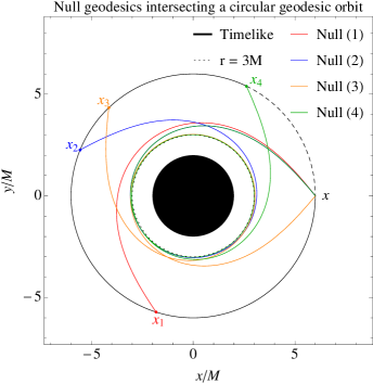
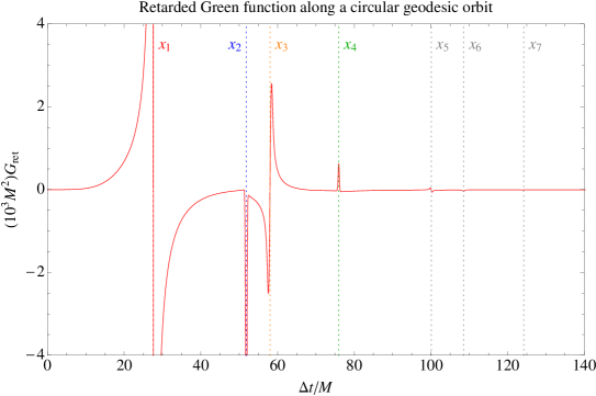
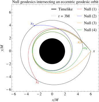
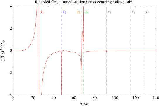
Figure 1: Green function along the innermost stable circular geodesic orbit of radius $r_{0}=6M$ (top) and along the eccentric geodesic orbit with $p=7.2,e=0.5$ at the point in the orbit where $r=6M$ and $\frac{dr(\tau)}{d\tau}>0$ (bottom). The left plots show the orbit and the first four null geodesics that start on the orbit, pass around the Schwarzschild black hole, and re-intersect the orbit. The right plot illustrates the retarded Green function $G_{\text{ret}}(x,x^{\prime})$ where $x^{\prime}$ is a point on the orbit a time $\Delta t$ in the past of $x$. The singular features at points $x_{1},x_{2},x_{3},\cdots$ correspond to the arrival of the null geodesics $(1),(2),(3),\cdots$ shown in the left plots. The singular features follow a four-fold repeating pattern, arising from the passage of the null wavefront through caustics.

In 1998, Poisson and Wiseman Poisson:Wiseman:1998 suggested a method for calculating the SF via Eq. (1) by using a method of matched expansions. Essentially, this method consists of splitting the tail integral in two different time regimes, as shown in Fig. 2. For times $\tau^{\prime}$ ‘close’ to $\tau$, in a region demarcated as the quasilocal (QL) region, the so-called Hadamard form for the GF is used. An advantage of this form is that the divergence of the GF at $\tau^{\prime}=\tau$ is explicit and so it is straightforward to remove it. The main disadvantage of this form is that it is only valid in a local neighbourhood of $z(\tau)$ and so a different method, typically a mode-sum expansion, must be used for times $\tau^{\prime}$ ‘far’ from $\tau$, in a region denoted as the distant past region (DP). A priori, it is not clear whether the two regions (QL region and DP) have a shared domain in which the expansions may be matched together. In Anderson:2005gb, the authors investigated the feasibility of the method of matched expansions for a scalar charge on Schwarzschild spacetime by using an approximation to the mode-sum expansion in the weak-field regime. In particular, they carried out a calculation of the SF in the QL region in the cases of a static charge and of a charge in a circular geodesic at radius $r=6M$ and, in the former case, of (a weak-field approximation to) the SF in the DP. They found that the convergence of the mode-sum method in the DP was “poor”, making matching between the calculations in the QL region and in the DP difficult to achieve. They concluded that this method is “promising but possessing some technical challenges”.

In Ref. Casals:2009zh we overcame some of these technical challenges to achieve the first successful calculation of SF with the method of matched expansions. This calculation was carried out on a static region of the Nariai spacetime ($dS_{2}\times\mathbb{S}^{2}$), which served as a toy-model for Schwarzschild spacetime. In this paper we extend the calculation in Ref. Casals:2009zh to the case of Schwarzschild spacetime. We calculate the SF on a scalar charge on Schwarzschild spacetime using a high-order expansion for the Hadamard form in the QL region, and a ‘full’ mode-sum expansion in the DP. We achieve good matching between the two calculations. The mode-sum expansion method consists of a spectral decomposition of the GF Leaver:1986; *PhysRevD.38.725 into its two main contributions: a sum over poles (the so-called quasinormal modes) and an integral around a branch cut on the negative-imaginary axis of the complex-frequency plane, as shown in Fig. 3. In other words, we calculate the full GF in Schwarzschild spacetime outside a local region by adding a quasinormal mode (QNM) contribution and a branch cut (BC) contribution. The BC contribution in Schwarzschild is a new addition with respect to the Nariai case, where the exponential fall-off of the radial potential ensures there is no BC and so the GF in the DP is fully given by the QNM contribution only.

We carry out the calculations using the method of matched expansions via the use of QL, QNM and BC contributions in the case of a scalar charge on Schwarzschild spacetime at $r=r_{0}\equiv 6M$ which is moving on (1) a circular geodesic (with angular velocity $\Omega=\sqrt{M}/r_{0}^{3/2}\approx 0.068/M$) and (2) an eccentric geodesic with $p=7.2$ and $e=0.5$, where $M$ is the mass of the black hole, $p$ is the semi-latus rectum and $e$ is the eccentricity. Figure 1 shows these two timelike geodesics; the null geodesics which re-intersect these orbits; and the GF along these orbits, calculated by the method of matched expansions presented.

The layout of the paper is as follows. In Sec. II we recap the method of matched expansions. In Secs. III and IV we describe the methods for calculating the GF in the QL region and DP, respectively. In Sec. LABEL:sec:matching we show the matching between the calculation in the QL region and in the DP. In Sec. LABEL:sec:SF we calculate the SF. We conclude the paper with a discussion in Sec. LABEL:sec:Discussion. Throughout, we use geometrized units, with $c=G=1$.

II The Method of Matched Expansions

As outlined in the Introduction, the method of matched expansions is a scheme for the direct evaluation of tail integrals such as Eq. (1). It was proposed fifteen years ago Poisson:Wiseman:1998, but until now it has not been developed into a practical scheme for SF calculation on a black hole spacetime. In this approach, the integral in Eq. (1) is split into two different time regimes, QL region and DP. In each regime the GF is obtained via a suitable expansion. If the expansions may be shown to share a common region of validity, then the tail integral may be evaluated. An overview of the method is given below, with technical details of the QL and DP expansions following in Secs. III and IV, respectively.

In summary, the method of matched expansions consists on calculating the SF via the expression

$$f_{\mu}(\tau)=q^{2}\nabla_{\mu}\left\{\int_{\tau_{m}}^{\tau^{-}}d\tau^{\prime}\ V(z(\tau),z(\tau^{\prime}))+\int_{-\infty}^{\tau_{m}}d\tau^{\prime}\ G_{\text{ret}}(z(\tau),z(\tau^{\prime}))\right\},$$ (2)

where $\tau_{m}$ is a properly chosen value of the proper time such that matching is possible between the QL (first term in Eq. (2)) and DP (second term in Eq. (2)) calculations. The method is schematically represented in Fig. 2.

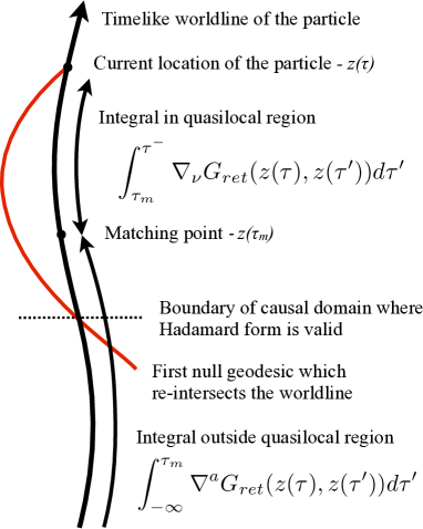
Figure 2: Schematic representation of the method of matched expansions (see Eq. (2)).

II.0.1 Green function in Hadamard form

The tail integral in Eq. (1) is taken along the entire past worldline, up to but not including the point of coincidence at $x=x^{\prime}$. The divergence of the GF at coincidence is explicitly manifest in the Hadamard form Friedlander; Hadamard; DeWitt:1960fc for the GF:

$$G_{\text{ret}}(x,x^{\prime})=\theta_{-}(x,x^{\prime})\left[U(x,x^{\prime})\delta(\sigma(x,x^{\prime}))-V(x,x^{\prime})\theta\left(-\sigma(x,x^{\prime})\right)\right],$$ (3)

where $U(x,x^{\prime})$ and $V(x,x^{\prime})$ are regular bitensors, $\delta$ and $\theta$ are the usual Dirac-delta and Heaviside distributions, respectively, and $\theta_{-}(x,x^{\prime})$ is equal to $1$ if $x$ lies to the future of $x^{\prime}$ and it is equal to $0$ otherwise. The two-point function $\sigma(x,x^{\prime})$ is Synge’s world-function, i.e., one-half of the square of the geodesic distance along the unique geodesic connecting the points $x$ and $x^{\prime}$. Because the Hadamard form exhibits an explicit form for the singularity of the GF at coincidence, it is trivial to remove this singular point from the integral (namely by subtracting the term with $U\delta(\sigma)$ from Eq. (3)).

The limitation of the Hadamard form Eq. (3) is that it is only valid in a convex normal neighbourhood of the base point $x$, that is, in a region $\mathcal{N}(x)$ containing $x$ with the property that every $x^{\prime}\in\mathcal{N}(x)$ is connected to $x$ by a unique geodesic which lies in $\mathcal{N}(x)$. This effectively requires that, in order to use the Hadamard form Eq. (3) for the GF in the SF expression Eq. (1), the worldline points $z(\tau)$ and $z(\tau^{\prime})$ must be connected by a unique nonspacelike geodesic which stays within $\mathcal{N}(z(\tau))$.

There are known uniformly convergent series which can be used to calculate $V(x,x^{\prime})$ DeWitt:1960fc; Friedlander throughout the domain of validity (i.e. for all $x^{\prime}\in\mathcal{N}(x)$), and methods for taking these series to very high order have been developed (see Sec. III). It remains to be shown that the convergence of such series is sufficiently rapid that an accurate calculation of $G_{\text{ret}}$ may be extended towards the boundary of $\mathcal{N}(x)$.

In Casals:2012px a method was proposed for calculating the GF globally by ‘propagating’ the Hadamard form to points $x^{\prime}$ outside $\mathcal{N}(x)$ via the use of Kirchhoff’s integral representation for the field. This method, however, requires a deep knowledge of the properties of $\sigma$, $U(x,x^{\prime})$ and $V(x,x^{\prime})$ which, in practice, makes the method difficult to apply to Schwarzschild spacetime.

II.0.2 Singular structure of Green function

Equation (3) shows that the singularities of $G_{\text{ret}}(x,x^{\prime})$ within $\mathcal{N}(x)$ occur not only at $x=x^{\prime}$ but also along $\sigma(x,x^{\prime})=0$, i.e., when the two spacetime points are connected by a null geodesic. It is known Garabedian; Ikawa that for $x^{\prime}$ outside $\mathcal{N}(x)$, the singularities of the GF continue to occur when the two spacetime points are connected by a null geodesic. The singularity of the GF for $x^{\prime}$ outside $\mathcal{N}(x)$ develops a structure which is richer than the solo Dirac-delta distribution exhibited for $x^{\prime}\in\mathcal{N}(x)$. It was recently shown Ori1short; Casals:2009zh; Dolan:2011fh; Harte:2012uw; Zenginoglu:2012xe; Casals:2012px that in various spacetimes the singularity of the GF when the spacetime points are null-separated exhibits a four-fold structure: $\delta(\sigma)$, $\text{PV}\left(1/\pi\sigma\right)$, $-\delta(\sigma)$, $-\text{PV}\left(1/\pi\sigma\right)$, $\delta(\sigma)$, …, where PV is the principal value distribution. The character of the singularity changes as the null geodesic crosses through a caustic point of the background spacetime. Such four-fold singularity structure was initially noted in General Relativity in Ori1short, first proven in Casals:2009zh in a static region of Nariai spacetime ($dS_{2}\times\mathbb{S}^{2}$), then shown in Schwarzschild spacetime in Dolan:2011fh, generalized in Harte:2012uw, proven in Plebański-Hacyan spacetime ($\mathbb{M}_{2}\times\mathbb{S}^{2}$) in Casals:2012px and physically explained as well as beautifully illustrated via numerical simulations in Schwarzschild spacetime in Zenginoglu:2012xe. We note that certain points in these spacetimes escape the previous singularity structure, such as points lying along a caustic line Dolan:2011fh; Casals:2012px; Zenginoglu:2012xe.

II.0.3 Multipole expansion

To move beyond the normal neighbourhood, one may expand the GF in multipoles and take a Fourier-mode decomposition. It was found in Anderson:2005gb that a lack of convergence of the sum over multipoles ($\ell$) and integral over frequency ($\omega$) presented a serious impediment to progress (convergence issues are somewhat inevitable, as the GF is a distribution with singular features). As described in the Introduction, a step forward came with writing the Fourier integral in terms of a quasinormal mode (QNM) sum (a sum of the residues of the GF at poles in the complex-frequency plane) Casals:2009zh, whose convergence properties are now well-understood (see Sec. IV.1). On a black hole spacetime, the expansion in QNMs must be supplemented by an integral along a branch cut, which has been the focus of some recent work (see Sec. IV.2).

III Quasilocal Expansion of the Green Function

In the QL region, the spacetime points $x$ and $x^{\prime}$ are assumed to be sufficiently close together that the GF is uniquely given by the Hadamard parametrix, Eq. (3). The term involving $U(x,x^{\prime})$ does not contribute to the integral in Eq. (1) since it has support only when $x=x^{\prime}$, and the integral excludes this point. We will therefore only concern ourselves in the QL region with the calculation of the function $V(x,x^{\prime})$.

The fact that $x$ and $x^{\prime}$ are close together suggests that an expansion of $V(x,x^{\prime})$ in powers of the separation of the points may give a good approximation within the QL region. Reference Casals:2009xa used a WKB method to derive such a coordinate expansion for spherically symmetric spacetimes and gave estimates of its range of validity. Referring to the results therein, we have $V(x,x^{\prime})$ as a power series in $(t-t^{\prime})$, $(1-\cos\gamma)$ and $(r-r^{\prime})$,

$$V(x,x^{\prime})=\sum_{i,j,k=0}^{\infty}v_{ijk}(r)~{}(t-t^{\prime})^{2i}(1-\cos\gamma)^{j}(r-r^{\prime})^{k},$$ (4)

where $\gamma$ is the angular separation of the points and $v_{ijk}$ are dimensionful coefficients. Note that — since $V(x,x^{\prime})$ is symmetric and the Schwarzschild spacetime is static — time reversal invariance ensures that only even powers of $(t-t^{\prime})$ can appear in this expansion. Up to an overall minus sign, Eq. (4) therefore gives the QL contribution to GF as required in the present context. It is also straightforward to take partial derivatives of these expressions at either spacetime point to obtain the derivative of the GF.

As proposed in Ref. Casals:2009xa, we have not used the QL expansion in the specific form of Eq. (4). Instead, we begin with an expansion of that form to 52-nd order in the coordinate separation and make two key modifications to improve both its accuracy and its domain of validity. Firstly, we factor out the leading form of the singularity at the first light crossing time. In the GF this singularity has the form $(t-t_{c})^{-1}$ and for the derivative of the GF it has the form $(t-t_{c})^{-2}$, where $t_{c}$ is the first light-crossing time. Secondly, we compute diagonal Padé approximants from the residual series expansions. In the circular orbit case, this second step is straightforward as all coordinates may be written in closed form in terms of the radius of the orbit and the time separation of the points. In the eccentric orbit case, we require the additional step of using the geodesic equations to rewrite the coordinates as expansions in $(t-t^{\prime})$ along the orbit, and then using the resulting series expansion for $V(z(\tau),z(\tau^{\prime}))$ in $(t-t^{\prime})$ alone as a starting point for computing a Padé approximant. The final result is an approximation for $V(z(\tau),z(\tau^{\prime}))$ in the form of a ratio of two polynomials in $(t-t^{\prime})$, with coefficients which are functions of $r$ only,

$$V(z(\tau),z(\tau^{\prime}))=\frac{\sum_{i=4}^{26}a_{i}(r)~{}(t-t^{\prime})^{i}}{(t-t_{c})\sum_{j=0}^{26}b_{j}(r)~{}(t-t^{\prime})^{j}}.$$ (5)

This expansion is an accurate representation of the GF throughout $\tau^{\prime}\in(0,\tau_{m}]$.

IV Spectral decomposition of the Green Function in the Distant Past

After a multipole-$\ell$ decomposition in the angular distance $\gamma$, the GF in Schwarzschild spacetime can be expressed as

$$G_{\text{ret}}(x,x^{\prime})=\sum_{\ell=0}^{\infty}\mathcal{G}^{ret}_{\ell},\quad\mathcal{G}^{ret}_{\ell}\equiv\frac{1}{r\,r^{\prime}}(2\ell+1)P_{\ell}(\cos\gamma)G^{\text{ret}}_{\ell}(r,r^{\prime};\Delta t),$$ (6)

where $r$ and $t$ are the radial and time Schwarzschild coordinates of the spacetime point $x$, respectively, and similarly $r^{\prime}$ and $t^{\prime}$ of the spacetime point $x^{\prime}$ and $\Delta t\equiv t-t^{\prime}$. By next carrying out a Fourier-mode decomposition in time, one obtains

$$G^{\text{ret}}_{\ell}(r,r^{\prime};\Delta t)\equiv\frac{1}{2\pi}\int_{-\infty+ic}^{\infty+ic}d\omega\ G_{\ell}(r,r^{\prime};\omega)e^{-i\omega\Delta t},$$ (7)

where $c>0$. The Fourier modes $G_{\ell}$ of the Green function satisfy the following second order radial ODE:

$$\left[\frac{d^{2}}{dr_{*}^{2}}+\omega^{2}-V(r)\right]G_{\ell}(r,r^{\prime};\omega)=-\delta(r_{*}-r^{\prime}_{*}),$$ (8)

$$V(r)\equiv\left(1-\frac{2M}{r}\right)\left[\frac{\ell(\ell+1)}{r^{2}}+\frac{2M}{r^{3}}\right],$$

together with appropriate retarded boundary conditions. Here, $r_{*}\equiv r+2M\ln\left(\frac{r}{2M}-1\right)$ is the radial ‘tortoise coordinate’. The Fourier modes of the GF can be calculated as

$$G_{\ell}(r,r^{\prime};\omega)=\frac{f_{\ell}(r_{<},\omega)g_{\ell}(r_{>},\omega)}{W\left(\omega\right)},$$ (9)

where $r_{>}\equiv\max(r,r^{\prime}),\ r_{<}\equiv\min(r,r^{\prime})$. The radial functions $f_{\ell}(r,\omega)$ and $g_{\ell}(r,\omega)$ are two linearly-independent solutions of the homogeneous version of the ODE (8). For $\text{Im}(\omega)\geq 0$ and $r_{*}/M\in\mathbb{R}$ they satisfy the boundary conditions:

$$f_{\ell}(r,\omega)\sim e^{-i\omega r_{*}}, r_{*}/M\to-\infty,$$ (10)

$$f_{\ell}(r,\omega)\sim A^{out}_{\ell,\omega}e^{+i\omega r_{*}}+A^{in}_{\ell,\omega}e^{-i\omega r_{*}}, r_{*}/M\to+\infty,$$

where $A^{in}_{\ell,\omega}$ and $A^{out}_{\ell,\omega}$ are complex-valued coefficients, and

$$g_{\ell}(r,\omega)\sim e^{+i\omega r_{*}},\quad\ r_{*}/M\to+\infty.$$ (11)

For $\text{Im}(\omega)<0$, with $r_{*}/M\in\mathbb{R}$, the solutions $f_{\ell}$ and $g_{\ell}$ must be defined by analytic continuation. The function

$$W\left(\omega\right)\equiv g_{\ell}f_{\ell}^{\prime}-f_{\ell}g_{\ell}^{\prime}=2i\omega A^{in}_{\ell,\omega},$$ (12)

where a prime indicates a derivative with respect to $r_{*}$, is the Wronskian of the two radial solutions.

In an influential paper, Leaver Leaver:1986; *PhysRevD.38.725 deformed the integral in Eq. (7) over (just above) the real axis on the complex-frequency plane to a contour along a high-frequency arc (HF) on the lower semiplane, as in Fig. 3. In doing so, the residue theorem of complex analysis dictates that one must take into account the singularities of the integrand. The Fourier modes $G_{\ell}$ possess simple poles (QNM frequencies) on the lower semiplane and a branch cut (BC) down the negative-imaginary axis on the complex-frequency plane. Therefore, the integral in Eq. (7) can be rewritten as a sum of the integral $G^{HF}_{\ell}$ along the high-frequency arc, a sum $G^{QN}_{\ell}$ over the residues at the poles, and an integral $G^{BC}_{\ell}$ around the branch cut:

$$G^{\text{ret}}_{\ell}=G^{HF}_{\ell}+G^{QN}_{\ell}+G^{BC}_{\ell}.$$ (13)

The QNM contribution $\mathcal{G}^{QN}_{\ell}$ and the BC contribution $\mathcal{G}^{BC}_{\ell}$ to $\mathcal{G}^{ret}_{\ell}$ are given by replacing $G^{\text{ret}}_{\ell}$ by, respectively, $G^{QN}_{\ell}$ and $G^{BC}_{\ell}$ in Eq. (6). The full QNM contribution $G_{QN}$ and the full BC contribution $G_{BC}$ to $G_{\text{ret}}$ are then respectively given by summing over all modes $G^{QN}_{\ell}$ and $G^{BC}_{\ell}$.

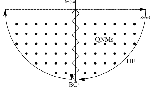
Figure 3: Contour deformation in the complex-frequency plane. The residue theorem of complex analysis allows one to re-express the integral over (just above) the real line of the Fourier modes $G^{\text{ret}}_{\ell}$ of the GF as an integral over a high-frequency arc (HF) plus an integral around a branch cut (BC) of the Fourier modes plus an integral over the residues at the poles (QNMs) of the Fourier modes.

The integral along the HF arc yields a ‘direct’ contribution which is expected to vanish after a certain finite time corresponding to a point $x^{\prime}$ not lying beyond the boundary of $\mathcal{N}(x)$ Ching:1994bd; Ching:1993gt; Ching:1995tj; Capon-1998. Furthermore, the quality of the match to the QL expansion in the region between $\Delta t\approx r_{*}+r^{\prime}_{*}$ and the edge of the normal neighbourhood is strong empirical evidence that it also doesn’t contribute there (at least in the specific cases investigated). We therefore will not be considering the HF contribution any further under the assumption that its contribution is either negligible or zero in the DP region.

In order to calculate the QNM and BC contributions $G_{QN}$ and $G_{BC}$, we mainly adopt the method introduced by Mano, Suzuki and Takasugi (MST) in Refs. Mano:1996vt; Mano:1996mf; Sasaki:2003xr (for the BC we also use other methods described below). In this approach, solutions to the radial equation are expressed via two complementary infinite series, using (i) Gaussian hypergeometric functions, and (ii) Coloumb wave functions. Formally, the radius of convergence of these series respectively extends towards (i) spatial infinity, and (ii) the event horizon. MST established the key relationships between these representations, which enable one to compute radial wave functions and derived quantities, such as the Wronskian, to high accuracy. MST’s method is particularly well-suited to calculations at low frequency.

In the next two subsections we give more details of the calculations of the QNM and BC contributions $G_{QN}$ and $G_{BC}$ and present the results. Further details on the calculational methods can be found in a series of papers Dolan:2011fh; Casals:2012tb; Casals:2012ng; Casals:Ottewill:2011smallBC; Dolan:Ottewill:QNMMST. We note that the plots in this section which depend on the orbit of the particle correspond only to the circular case with radius $r_{0}=6M$ since their features are essentially shared by the eccentric orbit case at the same radius with $p=7.2$ and $e=0.5$.

IV.1 Quasinormal Mode Sum

The Fourier modes $G_{\ell}$ of the GF have simple poles on the complex-frequency plane at the frequencies $\omega_{\ell n}$ where the Wronskian passes through zero. The condition $W(\omega_{\ell n})=0$ defines a discrete spectrum of quasi-normal modes, i.e. an infinite (but countable) set of complex frequencies $\omega_{\ell n}$ which are labelled by angular momentum $\ell$ and overtone $n$ numbers. The spectrum is symmetric under reflection in the imaginary axis, i.e. under $\omega_{\ell n}\rightarrow-\omega_{\ell n}^{\ast}$.

The key properties of the QNM spectrum can be understood by considering two asymptotic regimes. In the large angular momentum regime ($\ell\gg 1$ and $\ell\gg n$), the asymptotic spectrum is

$$\omega_{\ell n}\sim(\ell+1/2)\Omega-i(n+1/2)\Lambda,$$ (14)

where $\Omega$ and $\Lambda$ are, respectively, the orbital frequency and Lyapunov exponent (instability timescale) of the photon orbit at $r=r_{\text{orb}}$ 1972ApJ...172L..95G; PhysRevD.31.290 (known as the light-ring). For the Schwarzschild black hole, $\Omega=\Lambda=1/(\sqrt{27}M)$ and $r_{\text{orb}}=3M$. In the large overtone regime ($n\gg 1$ and $n\gg\ell$), the asymptotic spectrum is

$$\omega_{\ell n}\sim k-i\kappa(n+1/2).$$ (15)

Here $k$ is an $\ell$-independent constant which depends on the spin of the field, and $\kappa$ is the surface gravity at the horizon, $\kappa=1/(4M)$. For the scalar field on the Schwarzschild spacetime, $k=\ln(3)/(8\pi M)$ Andersson:2003fh.

We define $G^{QN}_{\ell}$ to be the sum of residues of the Fourier mode $G_{\ell}$ at its (simple) poles :

$$G^{QN}_{\ell}(r,r^{\prime};\Delta t)=\sum_{n=0}^{\infty}G^{QN}_{\ell,n}(r,r^{\prime};\Delta t),\quad G^{QN}_{\ell,n}(r,r^{\prime};\Delta t)\equiv 2\,\text{Re}\left(\frac{\mathcal{B}_{\ell n}}{\left(A^{out}_{\ell,n}\right)^{2}}f_{\ell}(r,\omega_{\ell n})f_{\ell}(r^{\prime},\omega_{\ell n})e^{-i\omega_{\ell n}\Delta t}\right),$$ (16)

where $A^{in/out}_{\ell,n}\equiv A^{in/out}_{\ell,\omega=\omega_{\ell n}}$. The QNM ‘excitation factors’ are defined by $\mathcal{B}_{\ell n}\equiv A^{out}_{\ell n}/(2\omega_{\ell n}\alpha_{\ell n})$ and $\alpha_{\ell n}$ is defined via $A^{in}_{\ell,\omega}\sim(\omega-\omega_{\ell n})\alpha_{\ell n}$ as $\omega\to\omega_{\ell n}$. We note that the radial function $g_{\ell}$ does not appear in Eq. (16) because it may be replaced by $f_{\ell}/A^{out}_{\ell,\omega}$ at a QNM frequency: the two quantities are equal when $\omega=\omega_{\ell n}$, as follows from the fact that $A^{in}_{\ell,n}=0$ and from the boundary conditions (10) and (11).

IV.1.1 QNM frequencies and excitation factors

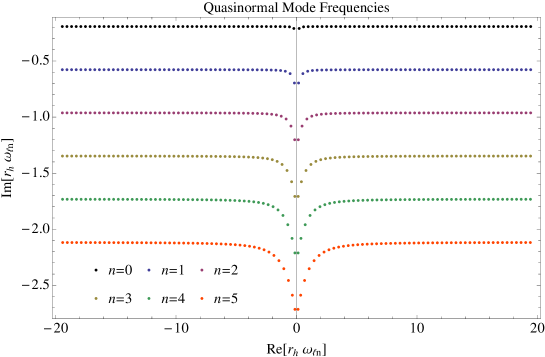
Figure 4: Scalar QNM frequencies in the complex-frequency plane in Schwarzschild spacetime for $n:0\to 5$ and $\ell:0\to 100$. The frequencies are symmetric with respect to the negative imaginary axis. In the 4th quadrant, the frequencies move down the plane with increasing $n$ and across to the right with increasing $\ell$.

Figure 4 shows the real and imaginary parts of the QNM frequencies $\omega_{\ell n}$ for $n:0\to 7$ and $\ell:0\to 100$. The plot demonstrates that the transition between the two asymptotic regimes is smooth. The imaginary part of the frequency remains negative for all $\ell$, $n$, indicating that all QNMs decay exponentially over time. As indicated by Eq. (14) and (15), the damping rate increases with overtone number. It is natural to call the lowest overtones ($n=0$) the ‘fundamental’ modes.

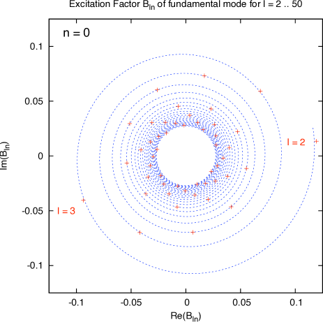
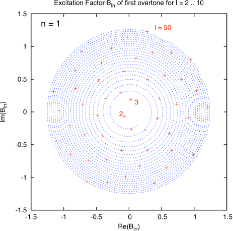
Figure 5: The QNM excitation factors in the Argand plane. These plots show the real and imaginary parts of $\mathcal{B}_{\ell n}$ for the fundamental ($n=0$, left) and first overtone ($n=1$, right) of the scalar field on Schwarzschild spacetime, from $\ell=2\ldots 50$. The data points show values determined with the MST method (see text), and the dotted lines show the asymptotic approximation for large $\ell$ (Eq. (31) in Ref. Dolan:2011fh).

Figure 5 shows the excitation factors $\mathcal{B}_{\ell n}$ determined via the MST method for the fundamental and first-overtone modes, for multipoles up to $\ell=50$. We have checked our values against the data in Tables III and IV of Ref. Berti:2006wq; against the asymptotic expressions in Ref. Dolan:2011fh; and against results from Ref. Zhang:2013ksa where the MST method is also used. In Appendix LABEL:sec:App we present tables with the QNM frequencies $\omega_{\ell n}$, the excitation factors $\mathcal{B}_{\ell n}$ and the coefficients $A^{out}_{\ell,n}$ for the modes $n=0\to 5$ and $\ell:0\to 50$.

IV.1.2 Convergence of mode sums

The sum over $n$ in Eq. (16) is taken over all QNMs in the fourth quadrant of the complex-$\omega$ plane. It is natural to ask whether this $n$-sum is convergent. Consider the case when $r$ and $r^{\prime}$ are large, so $f_{\ell}(r,\omega_{ln})\sim A^{out}_{\ell n}\exp(i\omega_{\ell n}r_{\ast})$ and we may write

$$G^{QN}_{\ell}(r,r^{\prime};\Delta t)\sim 2\,\text{Re}\sum_{n}C_{\ell,n}e^{-i\omega_{\ell n}T}$$ (17)

where $C_{\ell,n}$ can be read off from Eq.(16) and $T\equiv\Delta t-r_{\ast}-r_{\ast}^{\prime}$ is the ‘reflection time’. In the high overtone regime, the ratio of successive terms, $\sim|C_{\ell,n+1}/C_{\ell,n}|\exp(-\kappa T)$, is exponentially suppressed, via Eq. (15). It was demonstrated in Ref. Andersson:1996cm that for fixed $\ell$, $C_{\ell n}$ exhibits power-law dependence on $n$ at large $n$ and hence $T>0$ is a sufficient condition for the absolute convergence of the $n$-sum. In the general case, where $r$ and $r^{\prime}$ may not be large, the $n$-sum will still converge at sufficiently late times Casals:2011aa.

On the other hand, the sum over $\ell$ in Eq. (6) is not absolutely convergent, in any regime. Asymptotic expressions for the quantities featuring in Eq. (16) in the large-$\ell$ regime ($\ell\gg 1$, $\ell\gg n$) were given in Ref. Dolan:2011fh, in Eqs. (27)–(34) and (A41). In this regime, the magnitude of $\mathcal{B}_{\ell n}$ scales in proportion to $L^{n-1/2}/n!$, whereas the complex phase varies linearly with $L$, where $L\equiv\ell+1/2$.

It is is not a surprise to find that the series is not absolutely convergent, since we should recall that the GF is actually a distribution, which may exhibit infinitely-sharp features. The GF is singular on the light-cone. Conversely, we expect it to be well-defined and regular elsewhere. In Dolan:2011fh, using the large-$\ell$ asymptotic results, it was shown that (i) the solution of a coherent phase condition ($\lim_{\ell\rightarrow\infty}\text{arg}(G^{QN}_{\ell+1}/G^{QN}_{\ell})=2\pi k$ where $k\in\mathbb{Z}$) describes the light cone in spacetime, to within the expected error of the approximation; and (ii) the singularity structure of the GF follows a repeating four-fold pattern, as described in the Introduction: $\delta(\tilde{\sigma})$, $\text{PV}\left(1/\pi\tilde{\sigma}\right)$, $-\delta(\tilde{\sigma})$, $-\text{PV}\left(1/\pi\tilde{\sigma}\right)$, $\delta(\tilde{\sigma})$, …, where $\tilde{\sigma}$ is an approximation to Synge’s world-function $\sigma$. We next describe a method for obtaining well-defined values of the QNM $\ell$-sum for points lying in-between null geodesic reintersections.

IV.1.3 Calculation of mode sums

In order to perform the $\ell$-sum of the multipole modes $\mathcal{G}^{QN}_{\ell}$ we use the “smoothed sum method” of Sec. VII. D in Ref. Casals:2009zh, which is justified in Ref. Hardy. Our method relies on introducing a smoothing factor, $\tilde{S}(\ell)$, to attenuate the high-$\ell$ part of the mode sum.

As may be anticipated from Fourier theory, introducing a smooth filter in the $\ell$-mode decomposition is equivalent to convolving the GF with a narrow function which ‘smears out’ the distributional features. To make this precise, consider a distribution $D(\cdot)$ and a smooth function $S(\cdot)$ with mode sum representations

$$D(\cos\theta)=\sum_{\ell}\left(\ell+\frac{1}{2}\right)\tilde{D}(\ell)P_{\ell}(\cos\theta)\quad\quad\text{and}\quad\quad S(\cos\theta)=\sum_{\ell}\left(\ell+\frac{1}{2}\right)\tilde{S}(\ell)P_{\ell}(\cos\theta).$$ (18)

The smoothed mode sum is equivalent to a convolution of these functions, i.e.

$$\sum_{\ell}\left(\ell+\frac{1}{2}\right)\tilde{D}(\ell)\tilde{S}(\ell)P_{\ell}(\cos\theta)=\frac{1}{2\pi}\int_{-1}^{1}d(\cos\chi)\,\int_{-\pi}^{\pi}D(\cos\gamma)S(\cos\chi)d\varphi,$$ (19)

where $\cos\gamma=\cos\theta\cos\chi+\cos\varphi\sin\theta\sin\chi$.

We make use of a smoothing factor $\tilde{S}(\ell)\equiv\exp(-\ell^{2}/2\ell_{\rm cut}^{2})$. Via Eq. (18), this smoothing factor corresponds to a smearing function $S(\cos\theta)\sim L_{\rm cut}^{2}\exp(-L_{\rm cut}^{2}\theta^{2}/2)$ for small $\theta$, where $L_{\rm cut}=\ell_{\rm cut}+1/2$. It is straightforward to show that, in the limit $\ell_{\rm cut}\rightarrow\infty$, the smoothing factor smears a delta function, $\delta(\cos\theta-\cos\gamma)$, into a Gaussian $(L_{\rm cut}/\sqrt{2\pi\sin\theta\sin\gamma})\,\exp\left(-\frac{1}{2}L_{\rm cut}^{2}(\theta-\gamma)^{2}\right)$ of angular width $1/L_{\rm cut}$.

Such a smoothing factor can also be related to the numerical technique used in Zenginoglu:2012xe, where the four-dimensional Dirac-$\delta$ source in the PDE obeyed by the GF is replaced by a ‘narrow’ Gaussian distribution. If in Eq. (50) of Ref. Dolan:2011fh one introduces a smoothing factor $\tilde{S}(L)$ in the integrand, it is easy to show that the fourfold singularity structure of Eq. (52) Dolan:2011fh becomes ‘smoothed out’: instead of a Dirac-$\delta(\sigma)$ one obtains a Gaussian distribution and instead of the $\text{PV}\left(\frac{1}{\sigma}\right)$ type of singularity one obtains the Dawson integral of Eqs. (9) and (10) in Ref. Zenginoglu:2012xe with the width of the four-dimensional Gaussian being equal to $1/(M\ell_{\rm cut})$. That is, the introduction of a smoothing factor $\tilde{S}(L)$ in the $\ell$-sum is equivalent to a replacement of the four-dimensional Dirac-$\delta$ source by a Gaussian distribution.

In the circular orbit case we calculated up to 180 $\ell$-modes and in the eccentric orbit case up to 157 $\ell$-modes. For these values, we found it appropriate to take $\ell_{\rm cut}=25$. We have checked that, for large values of $\ell$, the modes $G^{QN}_{\ell}$ calculated via the method of MST agree well with the large-$\ell$ asymptotics obtained in Ref. Dolan:2011fh. We find that the large-$\ell$ asymptotics are accurate up to the expected level, i.e., up to terms of order $1/L$ in the complex phase. A small error in the phase can lead to a larger absolute error, particular for higher overtones, as $|\mathcal{B}_{\ell n}|\sim L^{n-1/2}$. For this reason, we have used only the results from the MST method.

IV.1.4 Sample MST results

Figure 6 shows the contribution of the lowest overtones to the GF, and its radial derivative, as a function of time along a circular geodesic. The plots shows that the higher overtones are negligible in comparison to the fundamental ($n=0$) modes for the majority of the time. This figure illustrates that the singularities of the QNM contribution $G_{QN}$ coincide precisely with the singularities of the full GF. That is, singular features in Fig. 6 occur whenever there is a null geodesic connecting the points on the worldline. These ‘light-crossing times’ (illustratively referred to as ‘caustic echos’ in Ref. Zenginoglu:2012xe) may be found by solving the null geodesic equations, and in the case of a circular geodesic at $r_{0}=6M$, the values are $\Delta t/M\approx 27.62,51.84,58.05,75.96,100.09,108.55,124.21,\dots$

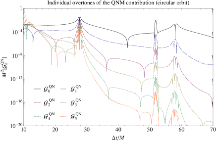
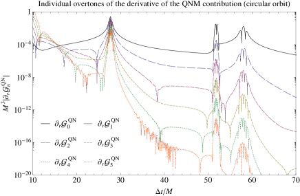
Figure 6: QNM contribution for individual overtones $n=0,1,2,3,4,5$ to the GF (left) and to the radial derivative of the GF (right) as a function of time $\Delta t$ along a circular geodesic of radius $r_{0}=6M$. Note that we use the symbol $\mathcal{G}_{n}^{QN}$ (with $G_{QN}=\sum_{n=0}^{\infty}\mathcal{G}_{n}^{QN}$, in obvious notation) in this figure only - not to be confused with $\mathcal{G}^{QN}_{\ell}$.

IV.2 Branch Cut

The BC integral $G^{BC}_{\ell}$ can be calculated as Casals:2011aa; Leung:2003ix

$$G^{BC}_{\ell}(r,r^{\prime};\Delta t)\equiv-\frac{i}{2\pi}\int_{0}^{\infty}d\nu\ \Delta G_{\ell}(r,r^{\prime};\nu)e^{-\nu\Delta t},$$ (20)

where $\nu\equiv i\omega>0$ along the BC, with the BC modes $\Delta G_{\ell}$ expressed as

$$\Delta G_{\ell}(r,r^{\prime};\nu)=-2i\nu f_{\ell}(r,-i\nu)f_{\ell}(r^{\prime},-i\nu)\frac{q(\nu)}{|W(-i\nu)|^{2}},\quad\text{for}\quad\frac{r_{*}}{M},\frac{r^{\prime}_{*}}{M}\in\mathbb{R},$$ (21)

where the function

$$q(\nu)\equiv-i\frac{\lim_{\epsilon\to 0^{+}}\left(g_{\ell}(r,\epsilon-i\nu)-g_{\ell}(r,-\epsilon-i\nu)\right)}{g_{\ell}(r,+i\nu)},$$ (22)

is the so-called branch cut ‘strength’. In order to calculate the BC contribution to the GF we used the methods recently developed in Casals:2012tb; Casals:Ottewill:2011smallBC; Casals:2012ng. We use a different method for three different frequency regimes along the BC: ‘very small’, ‘small’ and ‘mid’ frequency regimes. In the two orbit cases studied in this paper and for the values of $\ell$ included in the BC contribution, these regimes correspond to, respectively, $M\nu\in(0,0.05)$, $M\nu\in(0.05,0.225)$ and $M\nu\in(0.225,9)$.

It is clear from the exponential factor in Eq. (20) that the regime for ‘very small’ frequencies in the integral will only contribute significantly to $G^{BC}_{\ell}$ at ‘very late’ times. Due to this exponential factor, we need to carry out an analytic – rather than numeric – integration in this ‘very small’ frequency regime. We use the MST method in order to obtain the radial function $f_{\ell}$ and the functions $q(\nu)$ and $W(-i\nu)$. In order to perform a small-$|M\omega|$ expansion of the radial function $f_{\ell}$ we use the Barnes integral representation of the hypergeometric functions Casals:2012tb; Casals:Ottewill:2011smallBC, which appear in the MST series representations for $f_{\ell}$. We calculate the small-$|M\omega|$ expansion of $f_{\ell}$ up to three orders and of $q$ and $W$ up to fifteen orders (since the expansions for $q$ and $W$ are also used in the ‘small’ frequency regime). We found that a Padé approximation of the MST small-$|M\omega|$ expansion of the Wronskian $W$ significantly increases the validity of the expansion. It is shown in Casals:2012tb; Casals:Ottewill:2011smallBC that this ‘very small’ frequency regime yields the well-known Price:1972pw; Price:1971fb; Leaver:1986 power-law tail decay at late times of the GF plus a new logarithmic behaviour in time at higher order.

In the ‘small’ frequency regime, we use the same small-$|M\omega|$ expansions of $q$ and $W$ as those used in the ‘very small’ frequency regime. However, for the radial function $f_{\ell}$ itself we choose to use the Jaffé series Leaver:1986a; Casals:2012ng since it is easier to use and in this regime we do not need to carry out an exact analytic integration in Eq.(20).

In the ‘mid’ frequency regime we use the method developed in Casals:2012ng, since the convergence of the MST series representations becomes too slow in this regime as well as the fact that the coefficients in these series (which are the same as the coefficients in the Jaffé series) possess poles in this ‘mid’ frequency regime on the BC. The calculation of the BC modes in this ‘mid’ frequency regime enables us to see that, in the cases studied in this paper, the contribution of this regime to the BC is rather small but is necessary in order to increase the accuracy of the final value obtained for the SF.

In Fig. LABEL:fig:GBC_s=l=0_r=6 we show the contributions of these different frequency regimes along the BC to the radial derivative of $\mathcal{G}^{BC}_{\ell=0}$. Given how small the contribution from the ‘mid’ frequency regime is in the DP, in the cases we studied here the contribution from larger frequencies (i.e., $M\nu>9$ in the cases studied in this paper) is negligible and so we do not need to evaluate it (although asymptotics for ‘large’ frequency were developed in Casals:2011aa which could be used if necessary in other cases).