A certified reduction strategy for homological image processing

Abstract

The analysis of digital images using homological procedures is an outstanding topic in the area of Computational Algebraic Topology. In this paper, we describe a certified reduction strategy to deal with digital images, but preserving their homological properties. We stress both the advantages of our approach (mainly, the formalisation of the mathematics allowing us to verify the correctness of algorithms) and some limitations (related to the performance of the running systems inside proof assistants). The drawbacks are overcome using techniques that provide an integration of computation and deduction. Our driving application is a problem in bioinformatics, where the accuracy and reliability of computations are specially requested.

1 Introduction

Scientific computing is an outstanding tool to assist researchers in experimental sciences. When applied to biomedical problems, the accuracy and reliability of the computations are particularly important. Thus, the possibility of increasing the trust in scientific software by means of mechanized theorem proving technology becomes an interesting area of research.

In this paper, we explore this path to certify image processing procedures. In particular, we have chosen the Coq proof assistant [8] to certify the programs which allow us to analyse images obtained from neuron cultures [12]. The techniques that we use to deal with these images are based on Computational Algebraic Topology. Nowadays, computing in Algebraic Topology has an increasing importance in applied mathematics [17]; namely, in the context of digital image processing (see [4] and the series of conferences called Computational Topology in Image Context). The key observation of our approach is that, after a suitable preprocessing, the solution of a biological problem (namely, the number of synapsis in a picture of a neuron) can be identified with the computation of a topological invariant (the rank of a homology group). Then, all our efforts are concentrated on computing, in a certified manner, such an invariant.

Since the size of real-life biomedical images is too big to handle them directly, we propose a reduction strategy, that allows us to work with smaller data structures, but preserving all their homological properties. To this aim, we use the notion of discrete vector field [18], following very closely an algorithm due to Romero and Sergeraert [33].

In order to verify the correctness of these procedures, it is necessary the formalisation of a certain amount of mathematics. The most significant piece of mathematics formalised in this paper is the so-called Basic Perturbation Lemma (or BPL, in short). The proof of this theorem has been already implemented in the Isabelle/HOL proof assistant [1]. The BPL formalisation presented in this paper is much shorter and compact than that of [1]. There are two reasons for this improvement of the formal proof. The former is that in this work we have followed a new and shorter proof of the BPL (due again to Romero and Sergeraert [34]). The latter is that we have built our formal proof on the powerful SSReflect library of Coq [20] (on the contrary, much of the infrastructure required was defined from scratch in [1]).

Apart from the efficiency in the writing of proofs, using SSReflect also has other consequences. Since SSReflect is designed to deal only with finite structures, the proof of the BPL presented here only applies over finitely generated groups (the proof formalised in [1] has not this limitation). Furthermore, dealing with finite structures, and inside the constructive logic of Coq, eases the executability of the proofs, and thus the generation of certified programs (the same tasks in Isabelle/HOL pose more difficulties; see [2]). However, it is worth mention that this limitation does not mean any special hindrance in our work, because digital images are always finite structures.

In order to prove the correctness of the generated programs, we must establish, and keep, a link among the initial biomedical picture, and the final smaller data structure where the homological calculations are carried out. This implies a big amount of processing, and does not allow us to execute all the steps inside Coq (the full path has been travelled, but only in toy examples). Then we have appealed to a programming language, Haskell [27] in our case, to integrate computation and deduction.

Haskell appears in two different steps of our methodology. In the early stages of development, Haskell prototypes of the algorithms are systematically tested by using the QuickCheck tool [11]. This allows us to discharge many small and common errors, which could hinder the proving process in Coq. In the final computational step, Haskell is used as an oracle for Coq. The most hard parts of the calculation (in our case, an important bottleneck is computing inverse matrices) are delegated to Haskell programs; the results of these Haskell programs are then proved correct within Coq.

With this hybrid technique, we have got the objective of computing, in a certified way, the homology of actual biomedical images coming from neurological experiments.

The rest of this paper is organized as follows. Section 2 is devoted to present a running example, coming from the biomedical context, as a test-case for our development. The formalisation of an algorithm to build a discrete vector field associated with a matrix, using Coq and its SSReflect library, is explained in Section LABEL:dvf. This vector field computation will be used in Section 3 to reduce the chain complex associated with a digital image. The reduction process is based on an essential lemma in Algorithmic Homological Algebra called the Basic Perturbation Lemma. We also include in that section a proof of such a lemma. In Section 4, we explain how the certified programs can be used to effectively compute the homology of images. The paper ends with a section of conclusions and further work, and the bibliography.

The complete source code of our formalisation can be seen at http://www.unirioja.es/cu/cedomin/crship/.

2 Certified image processing

The discipline of Algebraic Digital Topology, or more specifically, the computation of homology groups from digital images is mature enough (see, for instance, [39], one among many good references) to go one step further and investigate the possibility of certified computations (i.e., computation formally verified by proving its correctness using an interactive proof assistant) in digital topology, as it happens in other areas of computer mathematics (see [19]).

In a very rough manner, the process to be verified is reflected in Figure 1. Putting it into words, we firstly pre-process a biomedical image to obtain a monochromatic image. From the black pixels of such a monochromatic image a cubical/simplicial complex is obtained (by means of a triangulation procedure); subsequently, from the cubical/simplicial complex, its boundary (or incidence) matrices are constructed, and finally, homology can be computed. If we work with coefficients over a field (and it is well-known that it is enough to take as coefficients the field $\mathbb{Z}_{2}$, when working with 2D and 3D digital images) and if only the degrees of the homology groups (as vector spaces) are looked for, then having a program able to compute the rank of a matrix is sufficient to accomplish the whole task. In this process the matrix obtained from the image can be huge. In this case, a process of reduction of the matrix without loosing the homological properties of the image can be applied previously to compute the homology. This architecture is particularised in this paper with a real problem that appeared in a biomedical application and with the Coq proof assistant and its SSReflect library as programming and verifying tool.

Figure 1: Computing homology from a digital image.

Biomedical images are a suitable benchmark for testing our programs, the reason is twofold. First of all, the amount of information included in this kind of images is usually quite big. Then, a process able to reduce those images but keeping the homological properties can be really useful. Secondly, software systems dealing with biomedical images must be trustworthy. This is our case since we have formally verified the correctness of our programs.

As an example, we can consider the problem of counting the number of synapses in a neuron. Synapses [7] are the points of connection between neurons and are related to the computational capabilities of the brain. The possibility of changing the number of synapses may be an important asset in the treatment of neurological diseases, such as Alzheimer, see [37]. Therefore, we can claim that an efficient, reliable and automatic method to count synapses is instrumental in the study of the evolution of synapses in scientific experiments.

Up to now, the study of the synaptic density evolution of neurons was a time-consuming task since it was performed, mainly, manually. To overcome this issue, an automatic method was presented in [25]. Briefly speaking, such a process can be split into two parts. Firstly, from three images of a neuron (the neuron with two antibody markers and the structure of the neuron), we obtain a monochromatic image, see Figure 2. In such an image, each connected component represents a synapse. So, the problem of measuring the number of synapses is translated into a question of counting the connected components of a monochromatic image.

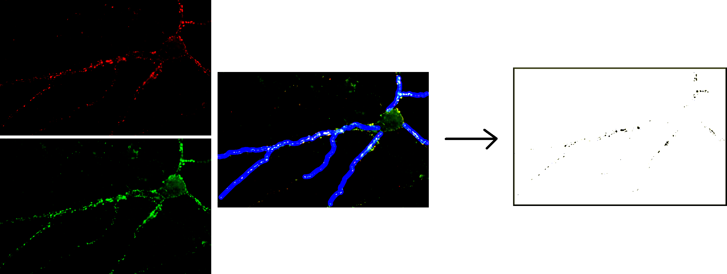
Figure 2: Synapses extraction from three images of a neuron.

In the context of Algebraic Digital Topology, this issue can be tackled by means of the computation of the homology group $H_{0}$ of the monochromatic image. This task can be performed in Coq through the formally verified programs which were presented in [24]. Nevertheless, such programs are not able to handle images like the one of the right side of Figure 2 due to its size. It is worth noting that Coq is a Proof Assistant and not a Computer Algebra system; and, in general, efficiency of algorithms is pushed into the background of this kind of systems. However, there is an effort towards the efficient implementations of mathematical algorithms running inside Coq, as shown by recent works on efficient real numbers [31], machine integers and arrays [3] or an approach to compiled execution of internal computations [21].

In our case, we apply a reduction process of the data structures but without loosing the homological properties to overcome the efficiency problem. In particular, we have focussed on the formalisation of discrete vector fields, a powerful notion that has been welcomed in the study of homological properties of digital images, see [10, 22, 29]. The importance of discrete vector fields, which were first introduced in [18], stems from the fact that they can be used to considerably reduce the amount of information of a discrete object but preserving homological properties. Using this approach, we can successfully compute the homology of the previous biomedical image in just $25$ seconds, a remarkable time for an execution inside Coq. Besides, we have proved using this proof assistant that the homological properties of the initial digital image and the reduced one are preserved.

In this section, we include the basic definitions which, mainly, come from the algebraic setting of Discrete Morse Theory presented in [33]. In addition, we present an algorithm to construct an admissible discrete vector field from a matrix. Then, a formalisation in Coq of this algorithm is provided. Finally, we introduce the fundamental notions in the Effective Homology theory [36] and state the theorem where Discrete Morse Theory and Effective Homology converge.

2.1 Basic mathematical definitions

We assume as known the notions of ring, module over a ring and module morphism (see, for instance, [28]). First of all, let us introduce one of the main notions in the context of Algebraic Topology: chain complexes.

Definition 1

A chain complex $C_{\ast}$ is a pair $(C,d)$, where $C=\{C_{n}\}_{n\in\mathbb{Z}}$ is a family of ${\mathcal{R}}$-modules and $d=\{d_{n}:C_{n}\rightarrow C_{n-1}\}_{n\in\mathbb{Z}}$ is family of module morphisms, called the differential map, such that $d_{n-1}\circ d_{n}=0$, for all $n\in\mathbb{Z}$. In many situations the ring ${\mathcal{R}}$ is either the integer ring, ${\mathcal{R}}=\mathbb{Z}$, or the field $\mathbb{Z}_{2}$. Usually, we denote the chain complex $C_{\ast}=(C_{n},d_{n})_{n\in\mathbb{Z}}$. A chain complex is free (finitely generated) if its modules are free (finitely generated).

The image $B_{n}=im~{}d_{n+1}\subseteq C_{n}$ is the (sub)module of $n$-boundaries. The kernel $Z_{n}=\ker d_{n}\subseteq C_{n}$ is the (sub)module of $n$-cycles. Given a chain complex $C_{\ast}=(C_{n},d_{n})_{n\in\mathbb{Z}}$, the identities $d_{n-1}\circ d_{n}=0$ mean the inclusion relations $B_{n}\subseteq Z_{n}$: every boundary is a cycle (the converse in general is not true). Thus the next definition makes sense.

Definition 2

The $n$-homology group of $C_{\ast}$, denoted by $H_{n}(C_{\ast})$, is defined as the quotient $H_{n}(C_{\ast})=Z_{n}/B_{n}$.

Chain complexes have a corresponding notion of morphism.

Definition 3

Let $C_{\ast}=(C_{n},d_{n})_{n\in\mathbb{Z}}$ and $D_{\ast}=(D_{n},\widehat{d}_{n})_{n\in\mathbb{Z}}$ be two chain complexes. A chain complex morphism $f:C_{\ast}\rightarrow D_{\ast}$ is a family of module morphisms, $f=\{f_{n}:C_{n}\rightarrow D_{n}\}_{n\in\mathbb{Z}}$, satisfying the relation $f_{n-1}\circ d_{n}=\widehat{d}_{n}\circ f_{n}$, for all $n\in\mathbb{Z}$. Usually, the sub-indexes are skipped, and we just write $f\circ d=\widehat{d}\circ f$.

Let us state now the main notions coming from the algebraic setting of Discrete Morse Theory [33].

Definition 4

Let $C_{\ast}=(C_{n},d_{n})_{n\in\mathbb{Z}}$ be a free chain complex with a distinguished $\mathbb{Z}$-basis $\beta_{n}\subset C_{n}$, for all $n\in\mathbb{Z}$. A discrete vector field $V$ on $C_{\ast}$ is a collection of pairs $V=\{(\sigma_{i},\tau_{i})\}_{i\in I}$ satisfying the conditions:

• Every $\sigma_{i}$ is some element of $\beta_{n}$, in which case $\tau_{i}\in\beta_{n+1}$. The degree $n$ depends on $i$ and in general is not constant.

• Every component $\sigma_{i}$ is a regular face of the corresponding $\tau_{i}$ (regular face means that the coefficient of $\sigma_{i}$ in $d_{n+1}(\tau_{i})$ is $1$ or $-1$).

• Each generator (cell) of $C_{\ast}$ appears at most one time in $V$.

It is not compulsory that all the cells of $C_{\ast}$ appear in the vector field $V$.

Definition 5

A cell $\chi$ which does not appear in a discrete vector field $V=\{(\sigma_{i},\tau_{i})\}_{i\in I}$ is called a critical cell. The elements $\sigma_{i}$ and $\tau_{i}$ in the vector field are called source and target cells, respectively.

From a discrete vector field $V$ on a chain complex, we can introduce the notion of $V$-paths.

Definition 6

A $V$-path of degree $n$ and length $m$ is a sequence $((\sigma_{i_{k}},\tau_{i_{k}}))_{0\leq k<m}$ satisfying:

• Every pair $(\sigma_{i_{k}},\tau_{i_{k}})$ is a component of $V$ and $\tau_{i_{k}}$ is an $n$-cell.

• For every $0<k<m$, the component $\sigma_{i_{k}}$ is a face of $\tau_{i_{k-1}}$ (the coefficient of $\sigma_{i_{k}}$ in $d_{n}(\tau_{i_{k-1}})$ is non-null) different from $\sigma_{i_{k-1}}$.

Definition 7

A discrete vector field $V$ is admissible if for every $n\in\mathbb{Z}$, a function $\lambda_{n}:\beta_{n}\rightarrow\mathbb{N}$ is provided satisfying the following property: every $V$-path starting from $\sigma\in\beta_{n}$ has a length bounded by $\lambda_{n}(\sigma)$.

In this way, infinite paths are avoided in an admissible discrete vector field. We will see that when a discrete vector field is admissible it is possible to distinguish the “useless” elements of the chain complex (in the sense, that they can be removed without changing its homology) and the critical ones (those whose removal could modify the homology).

If we consider the case of finite type chain complexes, where there is a finite number of generators in each degree, the differential maps can be represented as matrices. In that case, the problem of finding an admissible discrete vector field on the chain complex can be solved through the computation of an admissible vector field for those matrices.

Definition 8

Let $M$ be a matrix with coefficients in $\mathbb{Z}$, and with $m$ rows and $n$ columns. A discrete vector field $V$ for $M$ is a set of natural pairs $\{(a_{i},b_{i})\}_{i\in I}$ satisfying, for all $i\in I$, the following conditions:

• $1\leq a_{i}\leq m$ and $1\leq b_{i}\leq n$.

• $M[a_{i},b_{i}]=\pm 1$.

• The indexes $a_{i}$ (resp. $b_{i}$) are pairwise different.

When we work in a finite context the admissibility property is obtained if we avoid loops in the paths. Let $V$ be a vector field for a matrix $M$ with $m$ rows and $n$ columns. If $1\leq a,a^{\prime}\leq m$, with $a\neq a^{\prime}$ are two source cells, we can decide $a>a^{\prime}$ if there is an elementary $V$-path from $a$ to $a^{\prime}$, that is, if a vector $(a,b)$ is present in $V$ and $M[a^{\prime},b]$ is non-null. This means that $a$ is a regular face and $a^{\prime}$ is an arbitrary face of $b$. In this way, a binary relation is obtained on source cells. Then, the vector field $V$ is admissible if and only if this binary relation transitively generates a partial order, that is, if there is no loop $a_{1}>a_{2}>\ldots>a_{k}=a_{1}$.

2.2 Romero-Sergeraert’s algorithm

All the algorithms devoted to construct admissible discrete vector fields share the same goal: the construction of an admissible discrete vector field as big as possible (see for instance [30] or [38]). Some of them return a vector field quickly, but others spend more time to compute it. Let us emphasize that the latter ones are notable because the search has been more thorough, so the number of vectors will be higher. We are interested in an algorithm which not only gives us a big vector field but also does not spend too much time to compute it. The Romero-Sergeraert algorithm (from now on RS algorithm) does not always build the biggest vector field possible, but the number of vectors is quite close to the biggest one. Furthermore, in many cases, it returns the best possible vector field. Moreover, it is fast enough to obtain the vector field in our application domain. Due to these reasons, the RS algorithm has been chosen to make our computations.

Briefly, the RS algorithm builds an admissible discrete vector field running the rows of a matrix. It looks for the first element in the row which verifies the admissibility property with respect to the previously elements included in the discrete vector filed. We define the RS algorithm as follows.

Algorithm 9 (The RS Algorithm)

.
Input: a matrix $M$ with coefficients in $\mathbb{Z}$.
Output: an admissible discrete vector field $V$ for $M$ and a list of relations $r$.
Description:

1. Initialise the vector field $V$ to the void vector field and the relations $r$ to empty.

2. For every row $i$ of $M$:

   1. For every column $j$, which is different from the second components of $V$, such that $M[i,j]=1$ or $M[i,j]=-1$:

      • Look for the rows $k\neq i$ such as $M[k,j]\neq 0$ and obtain the relations $i>k$. Then, build the transitive closure of $r$ and these relations.

        • If there is no loop in that transitive closure:

          • then: Add $(i,j)$ to $V$, let $r$ be that transitive closure, and repeat from Step 2 with the next row.

          • else: Repeat from Step 2.1. with the next column.

In general, this algorithm can be applied over matrices with coefficients in a ring. In that case, the possible vectors will be only the elements whose value is a unit of the ring. Specifically, if we work with a field $F$, instead of a ring, every non-null element is a unit. In our particular case, as the homology groups of 2D images are torsion-free, we will work with the field $\mathbb{Z}_{2}$. Therefore, the selected vectors are entries whose value is $1$. From now on, we will work with $\mathbb{Z}_{2}$.

Let us mention that it is extremely relevant sorting the admissible discrete vector field because we will sort the matrix as a previous step to reduce it. For every vector $(a,b)$, the value of the function $\lambda(a)$, which gives us the longest path from $a$, is computed. In our case, as we build the transitive closure, it is the maximum length of the relations which start with $a$. Then, we sort the vector field by the values of $\lambda$ in decreasing order. Then, the rows and columns of the matrix are sorted using the ordered vector field. This matrix will have a lower triangular matrix with 1’s in the diagonal as upper-left submatrix of dimension the number of vectors in the vector field.

2.3 Formalisation of the RS algorithm in SSReflect

The development of a formally certified implementation of the RS algorithm was presented in [26]. It followed the methodology presented in [32]. Firstly, the programs were implemented in Haskell [27], a lazy functional programming language. Subsequently, our implementation was intensively tested using QuickCheck [11], a tool which allows one to automatically test properties about programs implemented in Haskell. Finally, the correctness of our programs were verified using the Coq [8] proof assistant and its SSReflect library [20]. In this section, we briefly show the last step of this process.

First of all, we define the data types related to our programs. A matrix is represented by means of a list of lists of the same length over $\mathbb{Z}_{2}$ (encoded using the unit ring type associated with the booleans), a vector field is a sequence of natural pairs, and finally, the relations are a list of lists of natural numbers. The notation a:T means that the variable a has type T.

⬇

Definition Z2:= bool_cunitRingType.

Record matZ2:=

{M: seq (seq Z2);

m: nat;

n: nat;

is_matrix: M = [::] \/

[/\ m = size M & forall i, i < m -> size (rowseqmx M i) = n]}.

Definition vectorfield:= seq (prod nat nat).

Definition rels:= seq(seq nat).

Then, we have defined a function called Vecfieldadm that checks if an element vf: vectorfield satisfies the properties of an admissible discrete vector field with respect to a matrix M: matZ2 and a list of relations r: rels.

⬇

Definition Vecfieldadm (M: matZ2)(vf: vectorfield)(r:rels):=

(all [pred i | 0<= i < (m M)](getfirstseq vf)) /\

(all [pred i | 0<= i < (n M)](getsndseq vf)) /\

(forall i j:nat, (i,j) \in vf -> (nth 0 (nth nil M i) j) = 1%R) /\

(uniq (getfirstseq vf)) /\

(uniq (getsndseq vf)) /\

(forall i j l:nat, (i,j) \in vf -> i!=l

-> (nth 0 (nth nil M l) j)!= 0%R -> (i::l::nil) \in r) /\

(forall a b s p, (a::s) \in r -> (last 0%N s = b)

-> (b::p) \in r -> ((a::s) ++ p) \in r) /\

(all uniq r) /\

(ordered glMax vf r).

Let us note that the first five conditions come from the three properties of a discrete vector field (see Definition 8). The next three conditions are linked with the relations. The first one gives us the link between the vector field and the relations. The second one verifies that we are constructing the transitive closure. And the last one states the admissibility property. It makes sure that every sequence of r has not repeated elements. Finally, it is checked that vf is ordered taking into account the glMax function, which returns the longest path associated with a cell, and the relations r.

The RS algorithm has been implemented using two functions: genDvf, which constructs an admissible discrete vector field, and genOrders, which generates the relations. As we have explained in the last paragraph of the previous subsection, the discrete vector field generated by the RS algorithms must be reordered, this is achieved thanks to the function dvford. The correctness of this program has been proved in the theorem dvfordisVecfieldadm – this theorem establishes that given a matrix M, the output produced by dvford satisfies the properties specified in Vecfieldadm.

⬇

Theorem dvfordisVecfieldadm (M:matZ2):

Vecfieldadm M (dvford M)(genOrders M).

The proof of the above theorem has been split into a series of lemmas which correspond with each one of the properties that should be fulfilled to have an admissible discrete vector field. For instance, the lemma associated with the first property of the definition of a discrete vector field is the following one.

⬇

Lemma propSizef (M:matZ2):

(all [pred i | 0 <= i < (size M)](getfirstseq (genDvf M)))

Both the functions which implement the RS algorithm and the ones needed to specify the properties of admissible discrete vector fields are defined using a functional style; that is, our programs are defined using pattern-matching and recursion. Therefore, in order to reason about our recursive functions, we need elimination principles which are fitted for them. To this aim, we use the tool presented in [6] which allows one to reason about complex recursive definitions in Coq.

For instance, in our development of the implementation of the RS algorithm, we have defined a function, called subm, which takes as arguments a natural number n and a matrix M and removes the first n rows of M. The inductive scheme associated with subm is set as follows.

⬇

Functional Scheme subm_ind := Induction for subm Sort Prop.

Then, when we need to reason about subm, we can apply this scheme with the corresponding parameters using the instruction functional induction. However, as we have previously said both our programs to define the RS algorithm and the ones which specify the properties to prove are recursive. Then, in several cases, it is necessary to merge several inductive schemes to induction simultaneously on several variables. For instance, let $M$ be a matrix and $M^{\prime}$ be a submatrix of $M$ where we have removed the $(k-1)$ first rows of $M$; then, we want to prove that $\forall j,\;M(i,j)=M^{\prime}(i-k+1,j)$. This can be stated in Coq as follows.

⬇

Lemma Mij_subM (i k: nat) (M: matZ2):

k <= i -> k != 0 -> let M’ := (subm k M) in

M i j == M’ (i - k + 1) j.

To prove this lemma it is necessary to induct simultaneously on the parameters i, k, and M, but the inductive scheme generated from subm only applies induction on k and M. Therefore, we have to define a new recursive function, called Mij_subM_rec, to provide a proper inductive scheme.

⬇

Fixpoint Mij_subM_rec (i k: nat) (M: matZ2) :=

match k with

|0 => M

|S p => match M with

|nil => nil

|hM::tM => if (k == 1)

then a::b

else (Mij_subM_rec p (i- 1) tM)

end

end.

This style of proving functional programs in Coq is the one followed in the development of the proof of Theorem dvfordisVecfieldadm.

2.4 Vector Field Reduction theorem

In this section, we state the theorem where Discrete Morse Theory and Effective Homology converge. First, we introduce reductions, one of the fundamental notions in the Effective Homology theory.

Definition 10

A reduction $\rho$ between two chain complexes $C_{\ast}=(C_{n},d_{n})_{n\in\mathbb{Z}}$ and $D_{\ast}=(D_{n},\hat{d}_{n})_{n\in\mathbb{Z}}$, denoted by $\rho:C_{\ast}\mbox{\,$\Rightarrow\Rightarrow$\,}D_{\ast}$, is a triple $\rho=(f,g,h)$ where $f:C_{\ast}\rightarrow D_{\ast}$ and $g:D_{\ast}\rightarrow C_{\ast}$ are chain complex morphisms, $h=\{h_{n}:C_{n}\rightarrow C_{n+1}\}_{n\in\mathbb{Z}}$ is a family of module morphism, and the following properties are satisfied:

1. $f\circ g=id$;

2. $g\circ f+d\circ h+h\circ d=id$;

3. $f\circ h=0$;  $h\circ g=0$;  $h\circ h=0$.

The importance of reductions lies in the fact that given a reduction $\rho~{}:~{}C_{\ast}\mbox{\,$\Rightarrow\Rightarrow$\,}D_{\ast}$, then $H_{n}(C_{\ast})$ is isomorphic to $H_{n}(D_{\ast})$ for every $n\in\mathbb{Z}$. Very frequently, $D_{\ast}$ is a much smaller chain complex than $C_{\ast}$, so we can compute the homology groups of $C_{\ast}$ much faster by means of those of $D_{\ast}$.

Theorem 11 (Vector Field Reduction Theorem)

Let $C_{\ast}=(C_{n},d_{n})_{n\in\mathbb{Z}}$ be a free chain complex and $V$ be an admissible discrete vector field on $C_{\ast}$. Then, the vector field $V$ defines a canonical reduction $\rho:(C_{n},d_{n})_{n\in\mathbb{Z}}\mbox{\,$\Rightarrow\Rightarrow$\,}(C^{c}_{n},d^{c}_{n})_{n\in\mathbb{Z}}$ where $C^{c}_{n}=\mathbb{Z}[\beta^{c}_{n}]$ is the free $\mathbb{Z}$-module generated by $\beta^{c}_{n}$, the critical $n$-cells of $C_{\ast}$.

Therefore, the bigger the admissible discrete vector field $V$ the smaller the chain complex $C^{c}_{\ast}$.

A quite direct proof of the Vector Field Reduction Theorem based on the Basic Perturbation Lemma appeared in [33].

Theorem 12 (Basic Perturbation Lemma, BPL)

Let $\rho=(f,g,h):(C,d)\mbox{\,$\Rightarrow\Rightarrow$\,}(\widehat{C},\widehat{d})$ be a reduction, and $\delta$ be a perturbation of $d$, that is, $\delta$ is a morphism such that $d+\delta$ is a differential map for $C$. Furthermore, the function $\delta\circ h$ is assumed locally nilpotent, in other words, for every $x\in C$ there exists $m\in\mathbb{N}$ (in general, $m$ can depend on $x$) such that $(\delta\circ h)^{m}(x)=0$. Then, a perturbation $\widehat{\delta}$ can be defined for the differential $\widehat{d}$ and a new reduction $\rho^{\prime}:(C,d+\delta)\mbox{\,$\Rightarrow\Rightarrow$\,}(\widehat{C},\widehat{d}+\widehat{\delta})$ can be constructed.

The proof of the Vector Field Reduction theorem based on the BPL is quite simple. Let us explain this proof in a nutshell. First of all, we consider a particular chain complex $(C,\delta)$ with the same underlying graded module than $(C,d)$, but with a simplified differential map. Namely, each component $\delta_{n}:C_{n}\rightarrow C_{n-1}$ is defined in the following way. It is clear that the vector field $V$ defines a canonical decomposition of $C_{n}$ depending on the generators are source, target, or critical cells. Then, $\delta_{n}$ apply to $0$ the source and critical cells. If $\tau$ is a target cell, there is a unique vector $(\sigma,\tau)\in V$. Then, $\delta_{n}(\tau)=\varepsilon(\sigma,\tau)\sigma$, where $\varepsilon(\sigma,\tau)$ is the coefficient $1$ or $-1$ of $\sigma$ in $d_{n}(\tau)$. A homotopy operator $h$ is defined in the same way as $\delta$ but in the reverse direction.

Then, we can define an initial reduction, $\rho=(f,g,h):(C,\delta)\mbox{\,$\Rightarrow\Rightarrow$\,}(C^{c},0)$, of the previous chain complex to the chain complex which modules are generated by the critical cells and which differential map is null. Now, let us define the morphism $P=(d-\delta)$ which is clearly a perturbation of $\delta$. If the nilpotency condition is satisfied, then the BPL produces the required reduction. The composition $(d-\delta)\circ h$ is not null only for source cells. For a source cell $\sigma$, the images $((d-\delta)\circ h)^{m}(\sigma)$ correspond to walking $V$-paths starting at this cell. As the vector field is admissible, the length of these paths is bounded, the image goes eventually to zero, and the nilpotency condition is obtained.

Again, in the case of finite type chain complexes which differentials are represented as matrices, given an admissible discrete vector field for those matrices, we can construct new matrices taking into account the critical components. These smaller matrices define chain complexes which preserve the homological properties. This is the equivalent version of Theorem 11 for finite type chain complexes. A detailed description of the process can be seen in [33].

3 Basic Perturbation Lemma

In this section, we introduce a formalisation in SSReflect of the BPL, a central lemma in Algorithmic Homological Algebra – in particular, it has been intensively used in the Kenzo Computer Algebra system [16]. In the literature, there are several ways of proving this lemma (see, for instance [5, 35]). There are also works related to the formalisation of the BPL. For instance, the non-graded case of this lemma is proved in Isabelle/HOL [1]. Furthermore, a particular case of the BPL is also proved in Coq using bicomplexes [15]. Now, we show a formalisation of the general case in SSReflect but with finitely generated structures. Let us recall that SSReflect only works with finite types; so, it can seem that this technology can restrict our development. Nevertheless, this approach is enough because we are interested in applying the BPL to the computation of the homology associated with a digital image – a case where every chain group is finitely generated. Indeed, in this context, this lemma is applied to a reduction where most of the differentials are null.

3.1 Mathematical proof of the BPL

The proof of the BPL (explained in [34]) is based on two results. The former, named Decomposition Theorem, builds a decomposition of a chain complex from a reduction of it. The latter is a Generalisation of the Hexagonal Lemma.

Theorem 13 (Decomposition Theorem)

Let $\rho=(f,g,h):(C,d)\mbox{\,$\Rightarrow\Rightarrow$\,}(\widehat{C},\hat{d})$ be a reduction. This reduction can be used to obtain a decomposition $C=A\oplus B\oplus C^{\prime}$ where: $C^{\prime}=im\;g$, $A\oplus B=\ker f$, $A=\ker f\cap\ker h$, $B=\ker f\cap\ker d$, the chain complex morphisms $f$ and $g$ are inverse isomorphisms between $C^{\prime}$ and $\widehat{C}$, and the arrows $d$ and $h$ are module isomorphisms between $A$ and $B$.

These properties are illustrated in the diagram represented in Figure 3.

Figure 3: Decomposition Theorem diagram.

It is a simple exercise of elementary linear algebra to prove the equivalence between the above diagram and the initial reduction.

The Hexagonal Lemma [33] allows us to reduce only a module of a chain complex in a particular degree. It is possible to generalize this lemma applying the reduction to every degree simultaneously.

Theorem 14 (Generalisation of the Hexagonal Lemma)

Let $C_{\ast}=(C_{n},d_{n})_{n\in\mathbb{Z}}$ be a chain complex. We assume that every module is decomposed $C_{n}=A_{n}\oplus B_{n}\oplus C^{\prime}_{n}$. The differential map $d_{n}$ are then decomposed in $3\times 3$ block matrices $[d_{n,i,j}]_{1\leq i,j\leq 3}$. If every component $d_{n,2,1}:A_{n}\rightarrow B_{n-1}$ is an isomorphism, then the chain complex can be canonically reduced to a chain complex $(C^{\prime}_{n},d^{\prime}_{n})$. The components of the desired reduction are:

$$\begin{array}[]{c}d^{\prime}_{n}=d_{n,3,3}-d_{n,3,1}d^{-1}_{n,2,1}d_{n,2,3}\;\;\;\;\;f_{n}=[\begin{array}[]{ccc}0&-d_{n,3,1}d^{-1}_{n,2,1}&1\end{array}]\\ \\ g_{n}=\begin{bmatrix}{-d^{-1}_{n,2,1}d_{n,2,3}}\\ {0}\\ {1}\end{bmatrix}\;\;\;\;h_{n-1}=\begin{bmatrix}{0}&{d^{-1}_{n,2,1}}&{0}\\ {0}&{0}&{0}\\ {0}&{0}&{0}\end{bmatrix}\end{array}$$

Again, it is not difficult to check that the displayed formulas satisfy the relations of a reduction stated in Definition 10.

With these two auxiliary lemmas, it is possible to obtain a proof of the BPL. The process is the following one. Given a reduction $\rho=(f,g,h):(C,d)\mbox{\,$\Rightarrow\Rightarrow$\,}(\widehat{C},\widehat{d})$ and a perturbation $\delta$ of the differential $d$ such that $\delta\circ h$ is locally nilpotent, it is necessary to build a new reduction $\rho^{\prime}=(f^{\prime},g^{\prime},h^{\prime}):(C,d+\delta)\mbox{\,$\Rightarrow\Rightarrow$\,}(\widehat{C},\widehat{d}+\widehat{\delta})$.

The reduction $\rho:C_{\ast}\mbox{\,$\Rightarrow\Rightarrow$\,}\widehat{C}_{\ast}$ allows us to apply the Decomposition Theorem and to obtain the diagram of Figure 3 where $C=A\oplus B\oplus C^{\prime}$. Then, the differential $(d+\delta)$ can be depicted in nine blocks following that decomposition. If the component $(d+\delta)_{21}:A\rightarrow B$ is invertible then the Generalisation of Hexagonal Lemma can be applied and the BPL is proved.

We have that $(d+\delta)_{21}=d_{21}+\delta_{21}=d_{21}+\delta_{21}\circ h_{12}\circ d_{21}=(id+\delta_{21}\circ h_{12})\circ d_{21}$. Then, as $d_{21}$ is invertible (in fact, $h_{12}$ is its inverse), we focus on proving that the other member of the product, namely $(id+\delta_{21}\circ h_{12})$, is invertible.

As $\delta\circ h$ is locally nilpotent, i.e. for every $x\in C$, there exists $m\in\mathbb{N}$ satisfying $(\delta\circ h)^{m}(x)=0$, we obtain that in particular $(\delta_{21}\circ h_{12})^{m}(x)=0$ since the unique non-null component of $h$ is $h_{12}$. Then, the inverse of $(id+\delta_{21}\circ h_{12})$ is $\sum_{i=1}^{\infty}(-1)^{i}(\delta_{21}\circ h_{12})^{i}$.

3.2 Formalisation of the BPL

The formalisation of the proof of the BPL in SSReflect requires to restrict the data structures to finitely generated chain complex. These structures are presented in Subsection 3.2.2. Then, the Decomposition Lemma and the Generalized Hexagonal Lemma are formalised in Subsection 3.2.3 and 3.2.4. These two results are the key ingredients used in the formalisation of the BPL – included in Subsection 3.2.5. Before that, we start providing a brief explanation about the formalisation of the kernel of a map in SSReflect. The representation chosen for this well-known notion in mathematics has important consequences in the rest of structures used in the formalisation of the proof.

3.2.1 The kernel of a map

The kernel of a finite map is defined by the kernel of the matrix which represents this map. This is defined in SSReflect in the following way.

⬇

Definition kermx m n (A: ’M_(m,n)): ’M_m

:= copid_mx (\rank A) *m invmx (col_ebase A).

The kernel of a matrix A is defined as the inverse of col_ebase (the extended column basis of A), with the top \rank A rows zeroed out – this is achieved thanks to the multiplication of such inverse by a square diagonal matrix with 1’s on all but the first \rank A coefficients on its main diagonal (copid_mx (\rank A)). In other words, the kernel of a matrix $A$ is a square matrix whose row space consists of all u such that u *m A = 0. This property is expressed in the following lemma.

⬇

Lemma mulmx_ker m n (A : ’M_(m, n)) : kermx A *m A = 0.

Two comments are required about this definition. Firstly, the kernel consists of the elements that are made null when they are applied to the left. In our previous mathematical definitions they are null when applied to the right. Secondly, in our development, we have chosen to delete the top \rank A null rows of the kernel. If we worked with the original definition, we would obtain partial identities instead of identities in some proofs.

⬇

Definition ker_min (m n : nat) (M : ’M_(m,n)) :=

(castmx ((Logic.eq_refl (m-\rank M)),(\rank M) + (m-(\rank M))) = m)

(row_mx (@const_mx _ (m-\rank M) (\rank M) 0) 1%:M)) *m (kermx M).

The previous definition consists of the product of a row matrix with the kernel. The row matrix is composed by a block of zeros with m-\rank M rows and \rank M columns and an identity matrix of dimension \rank M. Let us note that the cast (a coercion which allows us to change an entity of one data type into another) in the definition is necessary so that the product can be properly defined – (kermx M) and (row_mx (@const_mx _ (m-\rank M) (\rank M) 0) 1%:M)) have, respectively, types ’M_m and ’M_(m-\rank M, \rank M + m- \rank M); so, we cast the type of (row_mx (@const_mx _ (m-\rank M) (\rank M) 0) 1%:M)) to ’M_(m-\rank M, m) using the castmx function. Anyway, both definitions generate the same space as we can see in the following lemma.

⬇

Lemma ker_min_kermx (m n : nat) (M : ’M_(m,n)) :

(kermx M :=: (ker_min M))%MS.

3.2.2 Main mathematical structures

Let us define a finitely generated chain complex with elements in a field.

⬇

Variable K: fieldType.

Record FGChain_Complex :=

{m: Z -> nat;

diff: forall i: Z, ’M[K]_(m (i + 1), m i);

boundary: forall i: Z, (diff (i + 1)) *m (diff i) = 0}.

Some comments about this definitions are necessary. The chain complex definition contains a function denoted by m which obtains the number of generators for each degree. Then, we can define the differentials using the matrix representation of these maps forall i: Z, ’M[K]_(m (i + 1), m i). Two important design decisions have been included in this definition. Due to the definition of the kernel of a matrix in SSReflect we will work with transposed matrices. This implies that the product is also reversed. Furthermore, the degrees of the differentials have been increased in one unit. This is an alternative definition to the usual one which considers the differential in degree i as a function from degree i+1 to degree i [15]. It is clear that as we are considering the definition for all the integers, both definitions are equivalent. However, with our version, a Coq technical problem is easily avoided.

Now, we can define the notions of chain complex morphism and homotopy operator for the FGChain_Complex structure.

⬇

Record FGChain_Complex_Morphism (A B: FGChain_Complex) :=

{FG : forall i: Z, ’M[K]_(m A i, m B i);

FG_well_defined: forall i: Z, (diff A i) *m (FG i) = (FG (i+1)) *m (diff B i)}.

Record FGHomotopy_operator (A: FGChain_Complex) :=

{Ho: forall i:Z, ’M[K]_(m A i, m A (i+1)%Z)}.

With these previous structures, we can define the notion of a reduction for a finitely generated chain complex. Namely, it is a record FGReduction with two chain complexes C D: FGChain_Complex, two morphisms F: FGChain_Complex_Morphism C D, G: FGChain_Complex_Morphism D C, a homotopy operator H: FGHomotopy_operator C, and the five properties of the reduction. For instance, the second property is defined as ax2: forall i: Z, (FG F (i+1)) *m (FG G (i+1)) + (Ho H (i+1)) *m (diff C (i+1)) + (diff C i) *m (Ho H i) = 1%:M.

We are going to focus our attention on the (diff C i) *m (Ho H i) component of the definition of a reduction. This product is possible without casts. If we consider the mathematically equivalent definition with the differential in degree i as a matrix ’M_(m i,m(i-1)), then the corresponding component would be (diff C i) *m (Ho H (i-1)). In this case a cast would be required to transform elements in degree (i-1+1) into elements in degree i. Using such a definition this kind of casts would populate the development; however, using our alternative definition, we avoid the use of casts.

3.2.3 Formalisation of the Decomposition Theorem

In this subsection, we focus on proving the Decomposition Theorem. The powerful SSReflect library on matrices makes this development easier. Given a reduction rho: FGReduction K we define the decomposition of (C rho) through an isomorphism between the module with (m (C rho) i) generators and the module built from the sum of three set of generators. The first morphism of the isomorphism reflects a change of basis between both modules (where we work with the canonical basis in the first one) taking into account how the second one is divided:

⬇

Definition Fi_isom (i: Z):=

(col_mx (ker_min (row_mx (FG (F rho) (i+1)) (Ho (H rho) (i+1))))

(col_mx (ker_min (row_mx (FG (F rho) (i+1)) (diff (C rho) i)))

(FG (G rho) (i+1)))).

In this definition it is necessary to note that the row space of the column matrix col_mx A B is the sum of the row spaces of the matrices A and B, and that the intersection of kernels of two matrices A and B generates the same space that the kernel of a row matrix row_mx A B.

The definition of the inverse morphism Gi_isom is obtained knowing that it is a row matrix composed by three blocks and using the second property of the reduction definition.

Then, applying the change of basis to the source chain complex of the reduction (C rho) we obtain a new reduction between the decomposed chain complex and the second chain complex of the reduction (D rho). It is not difficult to prove that the components of that reduction are:

$${{{{{\text{\leavevmode\lstinline{{\lst@@@set@language\lst@@@set@numbers\lst@@@set@frame\lst@@@set@rulecolor\lst@@@set@language{\@listingGroup{ltx_lst_identifier}{D\textunderscore rho\textunderscore base}}{\@listingGroup{ltx_lst_space}{ }}{\@listingGroup{ltx_lst_identifier}{i}}}}}}=\left(\begin{array}[]{ccc}0&\text{\leavevmode\lstinline{{\lst@@@set@language\lst@@@set@numbers\lst@@@set@frame\lst@@@set@rulecolor\lst@@@set@language{\@listingGroup{ltx_lst_identifier}{D\textunderscore aux}}{\@listingGroup{ltx_lst_space}{ }}{\@listingGroup{ltx_lst_identifier}{i}}}}}}&0\\ 0&0&0\\ 0&0&\text{\leavevmode\lstinline{{\lst@@@set@language\lst@@@set@numbers\lst@@@set@frame\lst@@@set@rulecolor\lst@@@set@language{\@listingGroup{ltx_lst_identifier}{diff}}{\@listingGroup{ltx_lst_space}{ }}({\@listingGroup{ltx_lst_identifier}{D}}{\@listingGroup{ltx_lst_space}{ }}{\@listingGroup{ltx_lst_identifier}{rho}}){\@listingGroup{ltx_lst_space}{ }}({\@listingGroup{ltx_lst_identifier}{i}}+1)}}}}\end{array}\right)\;\;\;\;\;\text{\leavevmode\lstinline{{\lst@@@set@language\lst@@@set@numbers\lst@@@set@frame\lst@@@set@rulecolor\lst@@@set@language{\@listingGroup{ltx_lst_identifier}{F\textunderscore rho\textunderscore base}}{\@listingGroup{ltx_lst_space}{ }}{\@listingGroup{ltx_lst_identifier}{i}}}}}}=\left(\begin{array}[]{l}0\\ 0\\ \text{\leavevmode\lstinline{{\lst@@@set@language\lst@@@set@numbers\lst@@@set@frame\lst@@@set@rulecolor\lst@@@set@language{\@listingGroup{ltx_lst_identifier}{id}}}}}}\end{array}\right)$$

$${{{{\text{\leavevmode\lstinline{{\lst@@@set@language\lst@@@set@numbers\lst@@@set@frame\lst@@@set@rulecolor\lst@@@set@language{\@listingGroup{ltx_lst_identifier}{G\textunderscore rho\textunderscore base}}{\@listingGroup{ltx_lst_space}{ }}{\@listingGroup{ltx_lst_identifier}{i}}}}}}=\left(\begin{array}[]{ccc}0&0&\text{\leavevmode\lstinline{{\lst@@@set@language\lst@@@set@numbers\lst@@@set@frame\lst@@@set@rulecolor\lst@@@set@language{\@listingGroup{ltx_lst_identifier}{id}}}}}}\end{array}\right)\;\;\;\;\;\text{\leavevmode\lstinline{{\lst@@@set@language\lst@@@set@numbers\lst@@@set@frame\lst@@@set@rulecolor\lst@@@set@language{\@listingGroup{ltx_lst_identifier}{H\textunderscore rho\textunderscore base}}{\@listingGroup{ltx_lst_space}{ }}{\@listingGroup{ltx_lst_identifier}{i}}}}}}=\left(\begin{array}[]{ccc}0&0&0\\ \text{\leavevmode\lstinline{{\lst@@@set@language\lst@@@set@numbers\lst@@@set@frame\lst@@@set@rulecolor\lst@@@set@language{\@listingGroup{ltx_lst_identifier}{H\textunderscore aux}}{\@listingGroup{ltx_lst_space}{ }}{\@listingGroup{ltx_lst_identifier}{i}}}}}}&0&0\\ 0&0&0\end{array}\right)$$

These components directly reflect the structure included in Figure 3. Finally, the two isomorphisms included in that diagram are easily obtained from these components using the properties of the redefined reduction.

3.2.4 Formalisation of the Generalisation of the Hexagonal Lemma

The first step in the formalisation of the Generalisation of the Hexagonal Lemma is defining its hypotheses. As every module is divided into three parts, every differential consists of nine blocks.

⬇

Variables (m1 m2 m3: Z -> nat).

Variable Di: forall i: Z,

’M[K]_(m1(i+1)+(m2(i+1)+m3(i+1)), (m1 i)+((m2 i)+(m3 i))).

Hypothesis boundary: forall i:Z, Di (i+1) *m Di i = 0.

Definition CH:= Build_FGChain_Complex boundary.

We recall that we are working with transposed matrices. Consequently, the block $(1,2)$ of each differential, denoted by d12, will be an isomorphism.

⬇

Variable d12_1: forall i: Z, ’M[K]_(m2 i, m1 (i + 1)).

Hypothesis d12_invertible:

forall i: Z, (d12 (i+1)) *m (d12_1 (i+1)) = 1%:M /\

(d12_1 (i+1)) *m (d12 (i+1)) = 1%:M.

Afterwards, we define the morphisms fi and gi and the homotopy operator hi to build a reduction of the chain complex CH. These maps are detailed in the proof of Theorem 14. For instance, we define gi i = ((-(d32 i)*(d12_1 i)) 0 1). Let us remark that (gi i) is a matrix whose type is: ’M_(m3(i+1), m1(i+1)+m2(i+1)+m3(i+1)). In this way (gi i) is defined between the modules of degree (i+1) instead of the ones of degree i. This allows us to avoid casts as in the case of the definition of the differential. Then, the rest of the components of the reduction are defined accordingly. Finally, the proof of the reduction properties are obtained using essentially rewriting tactics, allowing us to build the required reduction rhoHL.

3.2.5 Putting together the pieces to obtain a formalisation of the BPL

In order to obtain a formalisation of the BPL, we, firstly, define the hypotheses of the lemma. Those are a reduction and a perturbation of the first chain complex of the reduction.

⬇

Variable K: fieldType.

Variable rho: FGReduction K.

Variable delta: forall i:Z, ’M[K]_(m (C rho)(i+1), m (C rho) i).

Hypothesis boundary_dp: forall i:Z,

(diff (C rho) (i+1) + delta (i+1)) *m (diff (C rho) i + delta i) = 0.

In addition, we will assume the nilpotency hypothesis. Let us note that pot_matrix is a function which we have defined to compute the power of a matrix.

⬇

Variable (n: nat).

Hypothesis nilpotency_hp: forall i: Z,

(pot_matrix (delta i *m Ho (H rho) i) n = 0).

With these hypotheses, we have to define a reduction from the chain complex with the differential of (C rho) perturbed by delta. Firstly, we apply the Decomposition Lemma over the reduction rho, this allows us to decompose each (diff (C rho) i) in the $9$ blocks given in the proof of the lemma (see Subsection 3.2.3). The isomorphism given by Fi_isom and Gi_isom are used to decompose the perturbation in $9$ blocks.

⬇

Definition deltai_new (i:Z):=

(Fi_isom rho (i+1)) *m (delta (i+1)) *m (Gi_isom rho i).

Let us note that the differential deltai_new has moved up one degree with respect to delta. In this way, we obtain a division in 9 blocks of the chain complex Di_pert i:= diff (C rho) (i+1) + delta(i+1).

Then, the Generalisation of the Hexagonal Lemma can be applied if the block $(1,2)$ of that chain complex is invertible. Following the chain of equalities included in the mathematical proof of this lemma, it is enough to prove that 1%:M + H_aux * deltai_new21 has an inverse. To this aim, the following lemma is useful – the lemma is proved using the powerful bigop library of SSReflect [9].

⬇

Lemma inverse_I_minus_M_big (M: ’M[R]_n): (pot_matrix M m = 0) ->

(\sum_(0<=i<m) (pot_matrix M i)) *m (1%:M - M) = 1%:M.

Now, applying the Generalisation of the Hexagonal Lemma rhoHL we build a reduction quasi_bpl of the decomposed and perturbed chain complex.

The Generalisation of the Hexagonal Lemma proved in Subsection 3.2.3 builds a reduction of the chain complex given as hypothesis but moved up in a degree. Moreover, the definition of Di_pert has required us to define it moved up in a degree more. To sum up, we have built a reduction from a perturbed chain complex but moved up two degrees Di_BPL_up i:= (C rho)(i+1+1)+ delta(i+1+1). Finally, in order to obtain a reduction rho_BPL from the initial chain complex (C rho) perturbed by delta, we can move down two degrees in the reduction obtained. For instance, the differentials are defined as Di_BPL i:= castmx(cast3 i,cast4 i)(Di_BPL_up(i-1-1)). In this way, we have avoided the use of casts derived from the degrees until the last step of the proof.

3.3 Using the BPL to reduce the chain complex associated with a digital image

Different ways to represent matrices exist in a system. In SSReflect, there are two available representations. The first one formalises a matrix as a function. This function determines every element of the matrix through two indices (for its row and its column). With this abstract representation it is not difficult to define different operations with matrices and prove properties of them. Indeed, an extensive library on matrices is provided in SSReflect. For this reason, this representation was chosen to prove the BPL. However, this representation is not directly executable, since this matrix definition is locked to avoid the trigger of heavy computations during deduction steps. To overcome this drawback, an alternative definition which represents matrices as lists of lists was introduced in [13]. This concrete representation allows us to define operations which can be executed within Coq. Due to this reason, this was the representation chosen for the implementation of the RS algorithm, see Subsection 2.3. In the negative side, proving properties using this representation is much harder, and we do not dispose of the extensive SSReflect library.

In order to combine the best of both representations, a technique was introduced in [13]. In that work, two morphisms are defined: seqmx_of_mx from abstract to concrete matrices and mx_of_seqmx from concrete to abstract matrices. The compositions of this morphisms are identities. In this way, it is proved that these two matrix representations are equivalent. Besides, these morphisms allow changing the representation when required. We are going to use that idea to prove the Vector Field Reduction Theorem for a chain complex generated from a digital monochromatic image.

The process begins by defining a new structure to represent a particular type of chain complexes, called by us truncated chain complex. They consist only of two matrices d1, d2: matZ2, whose product is null. These matrices are the only not null components in the differential map of a chain complex. In this way, the null elements of this chain complex are not included in this definition. Besides, these matrices are represented using computable structures. The companion notions of truncated chain complex morphism, truncated homotopy operator, and truncated reduction are also defined for this structure.

As an example of the previously mentioned technique, we include the following definitions of two functions to sort a matrix, one for matrices represented as lists, and another one for matrices represented as functions (an equivalence between them is also provided in our development).

⬇

Definition reorderM (s1 s2: seq nat)(M: matZ2):=

(take_columns_s s2 (take_rows_s s1 M)).

⬇

Definition reorder_mx (s1:’S_m)(s2:’S_n)(M:’M[R]_(m,n)):=

col_perm s2 (row_perm s1 M).

Although these two definitions seem similar they adopt different approaches. The first one uses simple types which are closer to a standard implementation in traditional programming languages. Indeed, that implementation is a direct translation of the one made in Haskell. We will use this version to reorder the structures when we need to compute with them. For instance, let chaincomplexd1d2 be an initial truncated chain complex which differential is given by d1: matZ2, with m rows and n columns, and d2: matZ2 with n rows and p columns. It corresponds with the representation of the initial digital image that we want to reduce. The first definition is used to obtain the ordered list of lists d1’ and d2’ after computing an ordered and admissible discrete vector field for d1.

The second definition uses the full power of dependent types and the structures and properties developed in the SSReflect library. We will use this version when we need to prove properties on the reordered structures. For instance, this definition is used to obtain the boundary property of the truncated chain complex chaincomplexd1’d2’, or to define an isomorphism between chaincomplexd1d2 and chaincomplexd1’d2’. Both proofs take profit of properties on permutations included in the library.

We introduce just another example of the use of this approach. We need to prove that the upper-left submatrix of d1’ is a lower triangular matrix (of dimension the number of vectors in the admissible vector field, m1) with 1’s on its diagonal. In this case, the proof needs reasoning on the functions included in the RS algorithm and a quite long battery of add-hoc lemmas on the computable structures are required. In a second step, we need to prove that this matrix has an inverse. This second proof is easy using the results included in the SSReflect library after changing the representation.

Now, if we want to apply the BPL, we need to build a chain complex from the ordered truncated chain complex chaincomplexd1’d2’. This process requires some technical steps: translate lists to SSReflect matrices, transpose the matrices, and complete with null matrices all the not provided components. In particular, from d’1 we define the following matrix d’1_trmx which type is ’M[K]_(m1+(m - m1),m1+(n - m1)):

⬇

Definition d’1_trmx :=

trmx((mx_of_seqmx (m1 + (m - m1)) (m1 + (n - m1)) d’1)).

Then, we build the differential of a chain complex, denoted by CC_ordered, in the following way:

⬇

Definition diff_m:= fun i:Z => match i as

z return ((fun z0 : Z => ’M_(m_m (z0 + 1), m_m z0)) z) with

|(-1)%Z => d0_m

|0%Z => d’1_trmx

|1%Z => d’2_trmx

|2%Z => d3_m

|3%Z => dn_m

|_ => dn_m

end.

We have to highlight the differentials d0_m and d3_m because they are matrices with rows and no columns or with columns and no rows. The rest of differentials will be matrices with no rows and no columns.

We will obtain a reduction of this initial chain complex CC_ordered applying the BPL to the following auxiliary reduction. Let us define a chain complex Dcc whose modules have the same rank than the modules of CC_ordered, and whose differential has only one not null component. This component of type ’M[K]_(m1+(m-m1),m1+(n-m1)) is defined by a matrix hat_d1 whose upper-left block is the identity matrix of dimension m1 and is null in the rest of its blocks. The reduced chain complex Ccc has modules whose ranks are determined by the critical cells found by the RS algorithm on d1. That is, the only not zero ranks are m-m1, n-m1, and l. The differential of this reduced chain complex is null. Then, it is easy to build a reduction between Dcc and Ccc having h_0 (extracted from the homotopy operator given by trmx hat_d1) as its unique non-null component.

Now, we define a perturbation delta_m of Dcc. The non-null components of this perturbation are:

⬇

Definition delta_1 := d’1_trmx - hat_d1.

Definition delta_2 := d’2_trmx.

Then, if we prove the nilpotency condition we can apply the BPL. This lemma directly obtains the required reduction of CC_ordered. The natural number which allows us to prove this property is m1.+2. As we are working with finite structures, this number can be taken as a uniform bound for which the nilpotency condition is verified for all the elements in the module.

⬇

Lemma nilpotency_hp_m : forall i:Z,

(pot_matrix(delta_m i *m (Ho (H reductionFG_gen) i))(m1.+2) = 0).

In the proof of this lemma, the only interesting case is when i=0, that is: pot_matrix (delta_1 *m h_0)(m1.+2) = 0. Expanding the definitions using blocks, we obtain that the only non-null blocks are pot_matrix (d11 - id)(m1.+2) and d21 *m pot_matrix(d11 - id) (m1.+1), where d11 and d21 are, respectively, the up-left and down-left blocks of d’1_trmx.

Then, it suffices to prove that pot_matrix(d11 - id)(m1.+1)=0. Let us recall that d11 is an upper triangular matrix with type ’M_m1. We define the notion upper_triangular_up_to_k which given a natural number k and a matrix M determines whether the matrix is an upper triangular matrix with 0’s under and on the k-th diagonal. This definition is formalised in SSReflect as follows.

⬇

Definition upper_triangular_up_to_k n k (M: ’M[F]_n) :=

forall (i j: ’I_n), j <= i + k -> M i j = 0.

We have developed a small library of properties on upper triangular matrices which includes the following generalisation of the lemma to prove.

⬇

Lemma upper_triangular_pot_matrix_n n (M: ’M[F]_n) :

upper_triangular_up_to_k 0 M -> (pot_matrix M n.+1) = 0.

The BPL allows us to define a reduction red_BPL of CC_ordered. In order to obtain a truncated reduction from this reduction we retrace the technical steps made to apply the BPL: extract from this reduction the non-null maps, apply the transpose operation, and change the matrix representation. For instance, the two components of the first truncated chain complex in the reduction are defined in the following way.

⬇

Definition d’1_trmx_trmx:= seqmx_of_mx (trmx (diff (C red_BPL) 0)).

Definition d’2_trmx_trmx:= seqmx_of_mx (trmx (diff (C red_BPL) 1)).

It is necessary to stress that the obtained big truncated chain complex is composed of the differentials where the transpose operation has been applied twice. Some casts are needed in a last step in order to build a truncated reduction of the chain complex chaincomplexd’1d’2.

Finally, to obtain the required reduction, it remains to compose the isomorphism between the truncated chain complex chaincomplexd1d2 obtained from a digital image to the ordered truncated chain complex chaincomplexd1’d2’ with the reduction built as explained in the last paragraph.

4 Certified computation of the homology associated with a digital image

We have previously explained that we cannot directly compute in Coq the homology of a chain complex produced by actual images as the one of Figure 2 due to its size. Nevertheless, this computation is possible with the reduced chain complex. From a theoretical point of view, our objective consists in developing a formal proof which verifies that both images have the same homology; this has been accomplished in the previous sections. But, as we are working in a constructive setting, we could also undertake the computation inside Coq of the reduced chain complex. In the development included in the previous sections, only the first step towards that reduction is executable: the calculation of an admissible discrete vector field. The reduced matrix is then obtained through the BPL, which uses not executable matrices (because we have worked with the matrix definition included in the SSReflect library in order to prove the BPL).

We have developed a proof of the BPL for general (finitely generated) chain complexes, providing a notable formalisation. Then we have applied it in a very particular situation: we consider truncated chain complexes obtained from digital images, and we obtain an admissible discrete vector field using the RS algorithm on one of the matrices $d1$ of the differential map. In this situation, it is possible to obtain a reduction of $d1$ using directly the Hexagonal Lemma [33]. This reduction is extended to the other matrix of the differential in order to preserve the boundary condition. Concretely, the initial matrix $d1$ is divided into 4 blocks and the reduced one is built by the formula $d22-d21*d11^{-1}*d12$. In order to obtain an executable version of that reduction we have also formalised this simplified proof using computable structures. With this version we are able to compute the whole process for toy examples.

When the size of the matrix grows, it is not possible to compute the full path directly inside Coq. But we can calculate, in a certified manner within Coq, the homology of the reduced matrix. That is the case of actual images as the one in Figure 2. In this case, the original matrix has dimensions $690\times 1400$ and the reduced one $97\times 500$. This reduced matrix has been obtained using the Haskell version of the algorithm formalised in Coq. With the current state of the running machinery in Coq, the system is not able to compute of the steps producing this reduced chain complex. The bottleneck of our development is the definition of the inverse of a matrix. Although we have used a specialized function to compute the inverse of a triangular matrix with 1’s on its diagonal, implemented in [14], the performance gain has not been enough in this particular application. Finally, the solution adopted was to use Haskell as an oracle. The process is the following. From the matrices of the chain complex of a digital image, we delegate in Haskell the computation of the reduced matrix and the matrices of the required reduction (they also include the inverse matrix in their definition). Then, these matrices are brought into Coq which obtains the homology (in 25 seconds) of the reduced matrix and automatically (using the vm_compute tactic) compute the proofs (in 8 hours) of the reduction between both matrices.

5 Conclusions and further work

In this paper, we have reported on a research providing a certified computation of homology groups associated with some digital images coming from a biomedical problem. The main contributions allowing us to reach this challenging goal have been:

• The implementation in Coq of Romero-Sergeraert’s algorithm [33] computing a discrete vector field for a digital image.

• The complete formalisation in Coq/SSReflect of a proof of the Basic Perturbation Lemma (to be compared with the one at [1]).

• A methodology to overcome the problems of efficiency related to the execution of programs inside proof assistants; in this approach the programming language Haskell has been used with two different purposes: as a fast prototyping tool and as an oracle.

As for future work, several problems remain open. The most evident one is obtaining a better performance in the process. This can be undertaken at three different levels. First, by using other algorithms to compute the main objects in our approach (discrete vector fields of digital images, inverses of matrices, and so on). Second, by implementing more efficient data structures, suitable for the theorem proving setting. Third, by improving the running environments in proof assistants.

Another line of research is to apply our methodology and techniques to other problems related to the homological processing of biomedical images. The best candidate is persistent homology, which has been already applied and formalised (see [23]). The project would be to study whether our reduction strategy can be also profitable in this new homological context.

References

- [1] J. Aransay, C. Ballarin, and J. Rubio. A Mechanized Proof of the Basic Perturbation Lemma. Journal of Automated Reasoning, 40(4):271–292, 2008.
- [2] J. Aransay, C. Ballarin, and J. Rubio. Generating certified code from formal proofs: a case study in homological algebra. Formal Aspects of Computing, 2(22):193–213, 2010.
- [3] M. Armand, B. Grégoire, A. Spiwack, and L. Théry. Extending Coq with imperative features and its application to SAT verification. In Proceedings 1st International Conference on Interactive Theorem Proving (ITP’10), volume 6172 of Lecture Notes in Computer Science, pages 83–98, 2010.
- [4] R. Ayala, E. Domínguez, A.R. Francés, and A. Quintero. Homotopy in digital spaces. Discrete Applied Mathematics, 125:3–24, 2003.
- [5] D. Barnes and L. Lambe. Fixed point approach to homological perturbation theory. Proceedings of the American Mathematical Society, 112(3):881–892, 1991.
- [6] G. Barthe and P. Courtieu. Efficient Reasoning about Executable Specifications in Coq. In Proceedings 15th International Conference on Theorem Proving in Higher Order Logics (TPHOLS’02), volume 2410 of Lecture Notes in Computer Science, pages 31–46, 2002.
- [7] M. Bear, B. Connors, and M. Paradiso. Neuroscience: Exploring the Brain. Lippincott Williams & Wilkins, 2006.
- [8] Y. Bertot and P. Castéran. Interactive Theorem Proving and Program Development. Coq’Art: The Calculus of Inductive Constructions. Springer, 2004.
- [9] Y. Bertot, G. Gonthier, S. Ould Biha, and I. Pasca. Canonical Big Operators. In Proceedings 21st International Conference on Theorem Proving in Higher Order Logics (TPHOLS’08), volume 5170 of Lecture Notes in Computer Science, pages 86–101, 2008.
- [10] F. Cazals, F. Chazal, and T. Lewiner. Molecular shape analysis based upon Morse-Smale complex and the Connolly function. In Proceedings 19th ACM Symposium on Computational Geometry (SCG’03), pages 351–360, 2003.
- [11] K. Claessen and J. Hughes. QuickCheck: A Lightweight Tool for Random Testing of Haskell Programs. In ACM SIGPLAN Notices, pages 268–279. ACM Press, 2000.
- [12] G. Cuesto et al. Phosphoinositide-3-Kinase Activation Controls Synaptogenesis and Spinogenesis in Hippocampal Neurons. The Journal of Neuroscience, 31(8):2721–2733, 2011.
- [13] M. Dénès, A. Mörtberg, and V. Siles. A Refinement Based Approach to Computational Algebra in Coq. In Proceedings 3rd International Conference on Interactive Theorem Proving (ITP’2012), volume 7406 of Lecture Notes in Computer Science, pages 83–98, 2012.
- [14] M. Dénès, A. Mörtberg, and V. Siles. CoqEAL, the Coq Effective Algebra Library, 2012. http://www-sop.inria.fr/members/Maxime.Denes/coqeal.
- [15] C. Domínguez and J. Rubio. Effective Homology of Bicomplexes, formalized in Coq. Theoretical Computer Science, 412:962–970, 2011.
- [16] X. Dousson, J. Rubio, F. Sergeraert, and Y. Siret. The Kenzo program. Institut Fourier, Grenoble, 1998. http://www-fourier.ujf-grenoble.fr/s̃ergerar/Kenzo/.
- [17] H. Edelsbrunner and J. L. Harer. Computational Topology: An Introduction. American Mathematical Society, 2010.
- [18] R. Forman. Morse theory for cell complexes. Advances in Mathematics, 134:90–145, 1998.
- [19] G. Gonthier. Formal proof - the four-color theorem. 55(11):1382–1393, 2008.
- [20] G. Gonthier and A. Mahboubi. An introduction to small scale reflection in Coq. Journal of Formal Reasoning, 3(2):95–152, 2010.
- [21] Benjamin Grégoire and Xavier Leroy. A compiled implementation of strong reduction. In Proceedings International Conference on Functional Programming 2002, pages 235–246. ACM Press, 2002.
- [22] A. Gyulassy, P.T. Bremer, B. Hamann, and V. Pascucci. A practical approach to Morse-Smale complex computation: Scalability and generality. IEEE Transactions on Visualization and Computer Graphics, 14(6):1619–1626, 2008.
- [23] J. Heras, T. Coquand, A. Mörtberg, and V. Siles. Computing Persistent Homology within Coq/SSReflect. To appear in ACM Transactions on Computational Logic, 2013.
- [24] J. Heras, M. Dénès, G. Mata, A. Mörtberg, M. Poza, and V. Siles. Towards a certified computation of homology groups for digital images. In Proceedings 4th International Workshoph on Computational Topology in Image Context (CTIC’2012), volume 7309 of Lecture Notes in Computer Science, pages 49–57, 2012.
- [25] J. Heras, G. Mata, M. Poza, and J. Rubio. Homological processing of biomedical digital images: automation and certification. In 17th International Conferences on Applications of Computer Algebra. Computer Algebra in Algebraic Topology and its applications session, 2011.
- [26] J. Heras, M. Poza, and J. Rubio. Verifying an algorithm computing Discrete Vector Fields for digital imaging. In Proceedings 19th Symposium on the Integration of Symbolic Computation and Mechanised Reasoning (Calculemus’2012), volume 7362 of Lecture Notes in Computer Science, pages 215–229, 2012.
- [27] G. Hutton. Programming in Haskell. Cambridge University Press, 2007.
- [28] N. Jacobson. Basic Algebra II. W. H. Freeman and Company, 1989.
- [29] G. Jerse and N. M. Kosta. Tracking features in image sequences using discrete Morse functions. In Proceedings 3rd International Workshop on Computational Topology in Image Context (CTIC’2010), volume 1 of Image A, pages 27–32, 2010.
- [30] D. Kozlov. Combinatorial Algebraic Topology. Springer, 2007.
- [31] R. Krebbers and B. Spitters. Computer Certified Efficient Exact Reals in Coq. In Proceedings Conferences Intelligent Computer Mathematics (CICM’2011), volume 6824 of Lecture Notes in Computer Science, pages 90–106, 2011.
- [32] A. Mörtberg. Constructive algebra in functional programming and type theory. In Mathematics, Algorithms and Proofs 2010, 2010.
- [33] A. Romero and F. Sergeraert. Discrete Vector Fields and Fundamental Algebraic Topology, 2010. http://arxiv.org/abs/1005.5685v1.
- [34] A. Romero and F. Sergeraert. Homological Perturbation Theorem and Eilenberg-Zilber vector field, 2012. http://www-fourier.ujf-grenoble.fr/s̃ergerar/Talks/12-06-Zurich-1.pdf.
- [35] J. Rubio and F. Sergeraert. Constructive Algebraic Topology, Lecture Notes Summer School on Fundamental Algebraic Topology. Institut Fourier, Grenoble, 1997. http://www-fourier.ujf-grenoble.fr/s̃ergerar/Summer-School/.
- [36] J. Rubio and F. Sergeraert. Constructive Algebraic Topology. Bulletin des Sciences Mathématiques, 126(5):389–412, 2002.
- [37] D. J. Selkoe. Alzheimer’s disease is a synaptic failure. Science, 298(5594):789–791, 2002.
- [38] H. Lopes T. Lewiner and G. Tavares. Applications of Forman’s discrete morse theory to topology visualization and mesh compression. Transactions on Visualization and Computer Graphics, 10(5):499–508, 2004.
- [39] D. Ziou and M. Allili. Generating Cubical Complexes from Image Data and Computation of the Euler number. Pattern Recognition, 35:2833–2839, 2002.