Symmetry properties and spectra of the two-dimensional quantum compass model

Abstract

We use exact symmetry properties of the two-dimensional quantum compass model to derive nonequivalent invariant subspaces in the energy spectra of $L\times L$ clusters up to $L=6$. The symmetry allows one to reduce the original $L\times L$ compass cluster to the $(L-1)\times(L-1)$ one with modified interactions. This step is crucial and enables: (i) exact diagonalization of the $6\times 6$ quantum compass cluster, and (ii) finding the specific heat for clusters up to $L=6$, with two characteristic energy scales. We investigate the properties of the ground state and the first excited states and present extrapolation of the excitation energy with increasing system size. Our analysis provides physical insights into the nature of nematic order realized in the quantum compass model at finite temperature. We suggest that the quantum phase transition at the isotropic interaction point is second order with some admixture of the discontinuous transition, as indicated by the entropy, the overlap between two types of nematic order (on horizontal and vertical bonds) and the existence of the critical exponent. Extrapolation of the specific heat to the $L\to\infty$ limit suggests the classical nature of the quantum compass model and high degeneracy of the ground state with nematic order.

I Introduction

Spin-orbital physics is a very exciting and challenging field of research within the theory of strongly correlated electrons. Tokura and Nagaosa (2000); Oleś et al. (2005); Khaliullin (2005); Oleś (2012) Well known examples of Mott insulators with active orbital degrees of freedom are two-dimensional (2D) and three-dimensional (3D) cuprates, Feiner et al. (1997); *Fei98; Brzezicki et al. (2012); *Brz13 manganites,Feiner and Oleś (1999); *Fei05 and vanadates.Khaliullin et al. (2001); *Hor08 These realistic models are rather complicated and difficult to investigate due to spin-orbital entanglement,Oleś (2012) including the one on superexchange bonds. Oleś et al. (2006); You (2012) A common feature of spin-orbital models is intrinsic frustration of the orbital superexchange which follows from the directional nature of orbital states and their interactions. The orbital interactions are frequently considered alone, leading to orbital ordered states,van der Brink et al. (1999); van den Brink (2004); van Rynbach et al. (2010) to valence bond crystal or to orbital pinball liquid exotic quantum states.Trousselet et al. (2012a)

We shall concentrate below on a generic and the simplest model which describes orbital-like superexchange, the so-called quantum compass model (QCM),Nussinov and van den Brink (2013) introduced long ago by Kugel and Khomskii.Kugel and Khomskii (1982) In this 2D model the coupling along a given bond is Ising-like, but different spin components are active along different bond directions. A frequently used convention is that interactions take the form $J_{x}\sigma_{i}^{x}\sigma_{j}^{x}$ and $J_{z}\sigma_{i}^{z}\sigma_{j}^{z}$ along $a$ and $b$ axis of the square lattice. The compass model is challenging already for classical interactions. Nussinov et al. (2004) Recent interest in this model is motivated by its interdisciplinary character as it plays a role in the variety of phenomena beyond the correlated oxides; is is also dual to recently studied models of $p+ip$ superconducting arrays,Nussinov and Fradkin (2005) namely to the Hamiltonian introduced by Xu and Moore,Xu and Moore (2004) and to the toric code model in a transverse field.Vidal et al. (2009) Its 2D and 3D version was studied in the general framework of unified approach to classical and quantum dualities Cobanera et al. (2010) and in the 2D case it was proved to be self-dual.Xu and Moore (2004) The QCM was also suggested as an effective description for Josephson arrays of protected qubits,Douçot et al. (2005) as realized in recent experiment.Gladchenko et al. (2009) Finally, it could describe polar molecules in optical lattices and systems of trapped ions. Milman et al. (2007)

First of all, the 2D QCM describes a quantum phase transition between competing types of one-dimensional (1D) nematic orders, favored either by $x$ or $z$ part of the Hamiltonian and accompanied by discontinuous behavior of the nearest-neighbor (NN) spin correlations, Khomskii and Mostovoy (2003) when anisotropic interactions are varied through the isotropic point $J_{x}=J_{z}$, as shown by high-order perturbation theory,Dorier et al. (2005) rigorous mathematical approach,You et al. (2010) mean field (MF) theory on the Jordan-Wigner fermions,Chen et al. (2007) and sophisticated infinite projected entangled-pair state (PEPS) algorithm. Orús et al. (2009) Thus, in the thermodynamic limit one of the involved interactions is intrinsically frustrated because the energy of bonds along one direction is minimized but the other is not. In fact, these bonds which do not contribute to the actual spin order give no energy gain and are totally ignored. Second, the quantum Monte-Carlo studies of the isotropic QCM proved that the nematic order remains stable at finite temperature up to $T_{c}=0.055J$ and the phase transition to disordered phase stays in the Ising universality class.Wenzel and Janke (2008) As shown by Douçot et al.,Douçot et al. (2005) the eigenstates of the QCM are twofold degenerate and the number of low-energy excitations scales as linear size of the system. Further on, it was proved by exact diagonalization of small systems that these excitations correspond to the spin flips of whole rows or columns of the 2D lattice and survive when a small admixture of the Heisenberg interactions is included into the compass Hamiltonian.Trousselet et al. (2010); *Tro12 The elaborated multiscale entanglement-renormalization ansatz (MERA) calculations, together with high-order spin wave expansion,Cincio et al. (2010) showed that the 2D QCM undergoes a second order quantum phase transition when the interactions are modified smoothly from the conflicting compass interactions towards classical Ising model. It has also been shownCincio et al. (2010) that the isotropic QCM is not critical in the sense that the spin waves remain gapful in the ground state, confirming that the order in the 2D QCM is not of magnetic type.

For further discussion of the properties of the 2D QCM it is helpful to recall the 1D case. The 1D generalized variant of the compass model with $z$-th and $x$-th spin component interactions that alternate on even/odd exchange bonds is strongly frustrated, similar to the 2D QCM. The 1D QCM can be solved exactly by an analytical method in two different ways. Brzezicki et al. (2007); Brzezicki and Oleś (2009a) We note that the 1D compass model is equivalent to the 1D anisotropic XY model, solved exactly in the seventies. Perk et al. (1975) An exact solution of the 1D compass model demonstrates that certain NN spin correlation functions change discontinuously at the point of a quantum phase transition (QPT) when both types of interactions have the same strength, similarly to the 2D QCM. This somewhat exotic behavior is due to the QPT occurring in this case at the multicritical point in the parameter space.Eriksson and Johannesson (2009) The entanglement measures, together with so called quantum discord in the ground state characterizing the quantumness of the correlations, were analyzed recently You and Tian (2008); You (2012) to find the location of quantum critical points and to show that the correlations between two pseudospins on even bonds are essentially classical in the 1D QCM. While small anisotropy of interactions leads to particular short-range correlations dictated by the stronger interaction, in both 1D and 2D compass model one finds a QPT to a highly degenerate disordered ground state when the competing interactions are balanced.

The purpose of this paper is to present the symmetry properties of the 2D compass model and their implications for the energy spectra. Exact properties of the 2D QCM were introduced in Refs. Brzezicki and Oleś, 2010a, b; Brzezicki, 2011. Here we concentrate ourselves on certain generic features and extensions which provide more insights into the physical properties of the QCM. We present several results which were not published until now — they give a rather complete description of the physical properties of the model. We apply the symmetry for obtaining numerical results for the QCM on small square clusters, including the $6\times 6$ cluster which becomes considerably easier within the present approach than by a Lanczos exact diagonalization (ED) in invariant subspaces of fixed $S^{z}$ which makes no use of the symmetry described below. This symmetry is of importance here in spite of remarkable progress in the ED studies performed recently on large systems. For example, $S=\frac{1}{2}$ Heisenberg model was studied recently on the kagome lattice with $N=42$ sites in the subspace with $S^{z}=0$.Nakano and Sakai (2011)

The paper is organized as follows. In Sec. II we focus first on special symmetries of the planar QCM, giving the spin transformations that bring the Hamiltonian into the block-diagonal (or reduced) form and confirm its self-duality (Sec. II.1). Next, in Sec. II.2, we derive the equivalence relations between these diagonal blocks (or invariant subspaces) following from the translational invariance of the original QCM Hamiltonian and show the multiplet structure of the invariant subspaces for $4\times 4$, $5\times 5$ and $6\times 6$ lattices in Sec. III.1 and in the Appendix. The study of symmetries culminates in unveiling the hidden symmetry of the ground state of the QCM, see Sec. III.2, and its consequences for the four-point correlation functions using another spin transformation. Next, in Sec. IV, we present the results of ED techniques applied to the QCM for lattices of the sizes up to $6\times 6$. Due to the complexity of the many-body problem which includes time-consuming implementation of symmetry properties of the 2D QCM, this can be regarded as the state-of-the-art implementation of ED, see Sec. IV.1. The results include ground state properties of the QCM such as: spin correlation functions and covariances of the local and nonlocal type in Sec. IV.2. In Sec. IV.3 we present the evolution of energy levels as a functions of anisotropy, and entanglement entropy of a row in the lattice. We study as well the density of states for the $6\times 6$ cluster and heat capacities of the systems of different size at the isotropic point, see Sec. IV.4. The paper is summarized briefly in Sec. V.

II Symmetry properties of the two-dimensional compass model

II.1 Block-diagonal Hamiltonian

We consider the anisotropic ferromagnetic QCM for pseudospins $\frac{1}{2}$ on a finite $L\times L$ square lattice with periodic boundary conditions (PBCs):

$${\cal H}(\alpha) = -J\sum_{i,j=1}^{L}\left\{(1-\alpha)X_{i,j}X_{i+1,j}+\alpha Z_{i,j}Z_{i,j+1}\right\}$$ (1)

$$= -(1-\alpha)H^{x}-\alpha H^{z}\,,$$

where $\{X_{i,j},Z_{i,j}\}$ stand for Pauli matrices at site $(i,j)$ of a 2D square lattice, i.e., $X_{i,j}\equiv\sigma_{i,j}^{x}$ and $Z_{i,j}\equiv\sigma_{i,j}^{z}$ components, interacting on vertical and horizontal bonds by $H^{x}$ and $H^{z}$, respectively. The coupling constant $J$ is positive and the sign factor $-1$ is introduced to provide comparable ground state properties for odd and even systems. In this section we set $J=1$. The parameter $\alpha\in[0,1]$ changes the anisotropy between horizontal ($H^{x}$) and vertical ($H^{z}$) interactions; the isotropic model is found at $\alpha=\frac{1}{2}$. In case of $L$ being even, this model is equivalent to the antiferromagnetic QCM.

One can easily construct a set of $2L$ operators which commute with the Hamiltonian but anti-commute with one another:Douçot et al. (2005)

$$P_{i}\equiv\prod_{j=1}^{L}\,X_{i,j},\hskip 19.91684ptQ_{j}\equiv\prod_{i=1}^{L}\,Z_{i,j}.$$ (2)

Below we will use as symmetry operations all

$$R_{i}\equiv P_{i}P_{i+1}$$ (3)

and $Q_{j}$ to reduce the Hilbert space; this approach led to the exact solution of the compass ladder.Brzezicki and Oleś (2009b) The QCM Eq. (1) can be written in a common eigenbasis of $\{R_{i},Q_{j}\}$ operators using spin transformations of the form:

$$X_{i,j} = \prod_{p=i}^{L}\tilde{X}_{p,j}\,,\hskip 28.45274pt\tilde{X}_{i,j}=X^{\prime}_{i,j-1}X^{\prime}_{i,j}\,,$$ (4)

$$Z_{i,j} = \tilde{Z}_{i-1,j}\tilde{Z}_{i,j}\,,\hskip 19.91684pt\tilde{Z}_{i,j}=\prod_{q=j}^{L}Z^{\prime}_{i,q}\,,$$ (5)

where $\tilde{Z}_{0,j}\equiv 1$ and $X^{\prime}_{i,0}\equiv 1$. After writing the Hamiltonian ${\cal H}(\alpha)$ of Eq. (1) in terms of primed pseudospin operators one finds that the transformed Hamiltonian,

$${\cal H}^{\prime}(\alpha)=-(1-\alpha)H^{\prime}_{x}-\alpha H^{\prime}_{z},$$ (6)

contains no $\tilde{X}_{L,j}$ and no $Z^{\prime}_{i,L}$ operators so the corresponding $\tilde{Z}_{L,j}$ and $X^{\prime}_{i,L}$ can be replaced by their eigenvalues $q_{j}$ and $r_{i}$, respectively.

The Hamiltonian ${\cal H}^{\prime}(\alpha)$ is dual to the QCM ${\cal H}(\alpha)$ Eq. (1) in the thermodynamic limit; we give here an explicit form of its transformed $x$-part:

$$H^{\prime}_{x} = \sum_{i=1}^{L-1}\left\{\sum_{j=1}^{L-2}X^{\prime}_{i,j}X^{\prime}_{i,j+1}+X^{\prime}_{i,1}+r_{i}X^{\prime}_{i,L-1}\right\}$$ (7)

$$+ P^{\prime}_{1}+\sum_{j=1}^{L-2}P^{\prime}_{j}P^{\prime}_{j+1}+rP^{\prime}_{L-1},$$

and the similar form for the $z$-part:

$$H^{\prime}_{z} = \sum_{j=1}^{L-1}\left\{\sum_{i=1}^{L-2}Z^{\prime}_{i,j}Z^{\prime}_{i+1,j}+Z^{\prime}_{1,j}+s_{j}Z^{\prime}_{L-1,j}\right\}$$ (8)

$$+ Q^{\prime}_{1}+\sum_{j=1}^{L-2}Q^{\prime}_{i}Q^{\prime}_{i+1}+sQ^{\prime}_{L-1},$$

where $s_{j}=q_{j}q_{j+1}$, $s=\prod_{j=1}^{L-1}s_{j}$ and $r=\prod_{i=1}^{L-1}r_{i}$, and new nonlocal operators,

$$P^{\prime}_{j}=\prod_{p=1}^{L-1}\,X^{\prime}_{p,j},\hskip 19.91684ptQ^{\prime}_{i}=\prod_{q=1}^{L-1}\,Z^{\prime}_{i,q},$$ (9)

originate from the PBCs. As we can see, the $z$-th part $H^{\prime}_{z}$ (8) follows from $H^{\prime}_{x}$ (7) by the lattice transposition, replacing $X^{\prime}_{i,j}\rightarrow Z^{\prime}_{i,j}$ and $r_{i}\rightarrow s_{j}=q_{j}q_{j+1}$. Ising variables $r_{i}$ and $s_{j}$ are the eigenvalues of the symmetry operators $R_{i}\equiv P_{i}P_{i+1}$ and $S_{j}=Q_{j}Q_{j+1}$.

Instead of the initial $L\times L$ lattice of quantum spins, one finds here $(L-1)\times(L-1)$ internal quantum spins with $2(L-1)$ classical boundary spins, which gives $L^{2}-1$ degrees of freedom. The missing spin is related to the $Z_{2}$ symmetry of the QCM and makes every energy level at least doubly degenerate. Although the form of Eqs. (7) and (8) is complex, the size of the Hilbert space is reduced in a dramatic wayBrzezicki (2010); Brzezicki and Oleś (2010b) by a factor $2^{2L-1}$ which makes it possible to perform easily exact (Lanczos) diagonalization of 2D $L\times L$ clusters up to $L=6$.

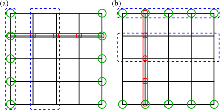
Figure 1: Panel (a): Schematic view of the $x$-th part of the effective compass Hamiltonian $H^{\prime}_{x}$ (7): open (green) circles are $X^{\prime}_{i,j}$ spin operators acting along first and last column, dashed (blue) frames indicate nonlocal $P^{\prime}_{j}$ spin operator products along columns and solid (red) frames are NN compass bonds $X^{\prime}_{i,j}X^{\prime}_{i,j+1}$. Panel (b): Schematic view of $H^{\prime}_{z}$ (8): open (green) circles are $Z^{\prime}_{i,j}$ spin operators acting along first and last line, dashed (blue) frames symbolize nonlocal $Q^{\prime}_{i}$ spin operator products along lines and solid (red) frames are NN compass bonds $Z^{\prime}_{i,j}Z^{\prime}_{i+1,j}$.

II.2 Equivalent subspaces

The spin transformations defined by Eqs. (4) and (5) bring the QCM Hamiltonian (1) into the block-diagonal form of Eqs. (7) and (8) with invariant subspaces labeled by the pairs of vectors $(\vec{r},\vec{s})$, with $\vec{r}=(r_{1},r_{2},\dots,r_{L-1})$ and $\vec{s}=(s_{1},s_{2},\dots,s_{L-1})$. The original QCM of Eq. (1) is invariant under the transformation $X\leftrightarrow Z$, if one also transforms the interactions, $\alpha\leftrightarrow(1-\alpha)$. This sets a relation between different invariant subspaces $(\vec{r},\vec{s})$, i.e., after transforming $\alpha\leftrightarrow(1-\alpha)$ the QCM Hamiltonian in subspaces $(\vec{r},\vec{s})$ and $(\vec{s},\vec{r})$ has the same energy spectrum. In general, we may say that the two subspaces are equivalent if the QCM has in them the same energy spectrum. This relation becomes especially simple for $\alpha=\frac{1}{2}$ when for all $r_{i}$’s and $s_{i}$’s subspaces $(\vec{r},\vec{s})$ and $(\vec{s},\vec{r})$ are equivalent.

Now we will explore another important symmetry of the 2D compass model reducing the number of nonequivalent subspaces — the translational symmetry. We note from Eqs. (7) and (8) that the reduced Hamiltonians are not translationally invariant for any choice of $(\vec{r},\vec{s})$ even though the original Hamiltonian is. This means that translational symmetry must impose some equivalence conditions among subspace labels $(\vec{r},\vec{s})$. To derive them, let us focus on translation along the rows of the lattice by one lattice constant. Such translation does not affect the $P_{i}$ symmetry operators, because they consist of spin operators multiplied along the rows, but changes $Q_{j}$ into $Q_{j+1}$ for all $j<L$ and $Q_{L}\rightarrow Q_{1}$. This implies that two subspaces $(\vec{r},q_{1},q_{2},\dots,q_{L})$ and $(\vec{r},q_{L},q_{1},q_{2},\dots,q_{L-1})$ are equivalent for all values of $\vec{r}$ and $\vec{q}$.

Now this result must be translated into the language of $(\vec{r},\vec{s})$ labels, with $s_{j}=q_{j}q_{j+1}$ for all $j<L$. This is two-to-one mapping because for any $\vec{s}$ one has two $\vec{q}$’s such that:

$$\vec{q}_{+} = (1,s_{1},s_{1}s_{2},\dots,s_{1}s_{2}\dots s_{L-1}),$$

$$\vec{q}_{-} = -\vec{q}_{+}\,.$$ (10)

The two values $\{q_{+},q_{-}\}$ differ by global inversion. This sets additional equivalence condition for subspace labels $(\vec{r},\vec{s})$: two subspaces $(\vec{r},\vec{u})$ and $(\vec{r},\vec{v})$ are equivalent if two strings $(1,u_{1},u_{1}u_{2},\dots,u_{1}u_{2}\dots u_{L-1})$ and $(1,v_{1},v_{1}v_{2},\dots,v_{1}v_{2}\dots v_{L-1})$ are related by translations or by a global inversion. For convenience, let us call this property of the two vectors a translation inversion (TI) relation. Lattice translations along the columns set the same equivalence condition for $\vec{r}$ labels. Thus full equivalence conditions for subspace labels of the QCM are:

• For $\alpha=\frac{1}{2}$ two subspaces $(\vec{r},\vec{s})$ and $(\vec{u},\vec{v})$ are equivalent if $\vec{r}$ is TI-related with $\vec{u}$ and $\vec{s}$ with $\vec{v}$ or if $\vec{r}$ is TI-related with $\vec{v}$ and $\vec{s}$ with $\vec{u}$.

• For $\alpha\not=\frac{1}{2}$ two subspaces $(\vec{r},\vec{s})$ and $(\vec{u},\vec{v})$ are equivalent if $\vec{r}$ is TI-related with $\vec{u}$ and $\vec{s}$ with $\vec{v}$.

We have verified that no other equivalence conditions exist between the subspaces by numerical Lanczos diagonalizations for lattices of sizes up to $6\times 6$, so we can change all if statements above into if and only if ones.

III Consequences of symmetry

III.1 Multiplets of equivalent subspaces: examples

For the finite square clusters of the sizes $4\times 4$, $5\times 5$ and $6\times 6$ we used the reduced form of the compass Hamiltonian to reduce the dimensionality of the Hilbert space and apply exact diagonalization techniques to get the ground state and thermodynamic properties of the QCM. For this purpose we needed to create a list of inequivalent subspaces for $L=4,5,6$ to save time and computational effort. According to the previous discussion let’s denote all inequivalent $\vec{r}$ configurations for our systems. For $L=4$ these fall into four TI-equivalence classes,

$$\begin{array}[]{cccc}\{\left[-+++\right],&\left[--++\right],&\left[-+-+\right],&\left[----\right]\}\end{array},$$

where the sign labels $q_{+}$ and $q_{-}$ in Eqs. (10), respectively. the number of different $\vec{q}$ labels that can be constructed out of each class is equal to the cardinality of this class divided by two. For the $4\times 4$ system these numbers are $\{4,2,1,1\}$. For $\vec{p}$ labels we have exactly the same set of classes so the subspace structure can be characterized by the following diagrams,

$$\begin{array}[]{cc}\begin{array}[]{cccc}16&8&4&4\\ 8&4&2&2\\ 4&2&1&1\\ 4&2&1&1\end{array}\,\,,&\hskip 56.9055pt\begin{array}[]{cccc}16&16&8&8\\ &4&4&4\\ &&1&2\\ &&&1\end{array}\,\,,\end{array}$$ (11)

where each number symbolizes an equivalence class of subspaces in anisotropic (left) and isotropic (right) cases and is equal to the number of subspaces in each class divided by two. As we see, the right diagram can be obtained from the left one by leaving diagonal numbers untouched, removing subdiagonal numbers and doubling the upper ones.

For $5\times 5$ we have again four TI–equivalence classes,

$$\{\left[-++++\right],\left[--+++\right],\left[-+-++\right],\left[-----\right]\},$$

with half-cardinalities $\{5,5,5,1\}$. This leads to the following diagrams,

$$\begin{array}[]{cc}\begin{array}[]{cccc}25&25&25&5\\ 25&25&25&5\\ 25&25&25&5\\ 5&5&5&1\end{array}\,\,,&\hskip 56.9055pt\begin{array}[]{cccc}25&50&50&10\\ &25&50&10\\ &&25&10\\ &&&1\end{array}\,\,.\end{array}$$ (12)

Finally, for the largest system considered here of $L=6$, the TI–equivalence classes read,

$$\begin{array}[]{cccc}\{\left[-+++++\right],&\left[--++++\right],&\left[-+-+++\right],\\ \left[--++-+\right],&\left[---+++\right],&\left[-++-++\right],\\ \left[+-+-+-\right],&\left[------\right]\},\end{array}$$ (13)

with half-cardinalities $\{6,6,6,6,3,3,1,1\}$, yielding the anisotropic diagram of the form,

$$\begin{array}[]{cccccccc}36&36&36&36&18&18&6&6\\ 36&36&36&36&18&18&6&6\\ 36&36&36&36&18&18&6&6\\ 36&36&36&36&18&18&6&6\\ 18&18&18&18&9&9&3&3\\ 18&18&18&18&9&9&3&3\\ 6&6&6&6&3&3&1&1\\ 6&6&6&6&3&3&1&1\end{array}\,.$$ (14)

The isotropic diagram can be obtained using the known procedure. These examples show that the number of inequivalent subspaces $N$ stays the same for the systems of sizes $L=2l$ and $L=2l+1$ (with $l=1,2,3,\dots$) and is directly related to the number $n$ of TI–equivalence classes of the binary string of the length $L$. We have:

$$N=\begin{cases}n^{2}&for\qquad\;\alpha\neq\frac{1}{2},\\ \frac{1}{2}n(n+1)&for\qquad\;\alpha=\frac{1}{2}.\end{cases}$$ (15)

The most numerous TI-equivalence class for the $L\times L$ system consists of the binary strings which transform into themselves after $L$ translations, so carrying highest number of possible pseudomomenta. This implies that largest subspace equivalence class contains $2L^{2}$ subspaces in anisotropic and $4L^{2}$ subspaces in isotropic case. Knowing that the total number of subspaces is $2\times 2^{2(L-1)}$ one can estimate that $N>2^{2(L-1)}L^{-2}$ for $\alpha\not=\frac{1}{2}$, and $N>2^{2L-3}L^{-2}$ for $\alpha=\frac{1}{2}$.

III.2 Hidden order

Due to the symmetries of the QCM Eq. (1) only $\langle Z_{i,j}Z_{i,j+d}\rangle$ and $\langle X_{i,j}X_{i+d,j}\rangle$ two-point spin correlations are finite ($d\geq 1$). This suggests that the entire spin order concerns pairs of spins from one row (column) which could be characterized by four–point correlation functions of the dimer-dimer type. Such correlations are presented in form of the $2d$ point $\langle XXXX\rangle$ correlation function in Fig. 2(a) and by dimer-dimer correlations in Fig. 2(b). Indeed, examining such quantities for finite QCM clusters via Lanczos diagonalization we observed certain surprising symmetry: for any $\alpha$ two dimer-dimer $\langle(XX)_{1}(XX)_{2}\rangle$ correlators are equal under the quasi-reflection along the local diagonal as shown in Fig. 2(b). This property turns out to be a special case of a more general relation between correlation functions of the QCM which we prove below.

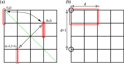
Figure 2: Example of application of the proved identities in two cases: (a) — Eq. (22) long range correlation function $\langle X_{i,j}X_{i+d+1,j}\rangle$ along the column (circles) is equal to the $2d$–point $\langle XX\dots X\rangle$ correlation function along the row (solid (red) frame of length $d$); (b) — Eq. (21) for two chosen dimers at $(i,j)$ and $(k,l)$ (solid frames), correlations between them are the same as between dimers at $(i,j)$ and $(k-\delta,l+\delta)$ (dashed frame). Green dashed line marks the plane of the mirror reflection transforming site $(k,l)$ into $(k-\delta,l+\delta)$.

We will prove that in the ground state of the QCM for any two sites $(i,j)$ and $(k,l)$ and for any $\alpha\in(0,1)$:

$$\langle X_{i,j}X_{i+1,j}X_{k,l}X_{k+1,l}\rangle\equiv\quad\quad\quad$$

$$\langle X_{i,j}X_{i+1,j}X_{l-\delta,k+\delta}X_{l-\delta+1,k+\delta}\rangle,$$ (16)

where $\delta=j-i$. To prove Eq. (16) let us transform again the effective Hamiltonian (7) in the ground state subspace ($r_{i}\equiv s_{i}\equiv 1$) introducing new spin operators,

$$Z^{\prime}_{i,j}=\tilde{Z}_{i,j}\tilde{Z}_{i,j+1},\hskip 28.45274ptX^{\prime}_{i,j}=\prod_{r=1}^{j}\tilde{X}_{i,r},$$ (17)

with $i,j=1,\dots,L-1$ and $\tilde{Z}_{i,L}\equiv 1$. This yields

$$\tilde{H}_{x}=\sum_{i,j=1}^{L-1}\!\tilde{X}_{i,j}+\prod_{i,j=1}^{L-1}\!\tilde{X}_{i,j}+\sum_{i=1}^{L-1}\prod_{j=1}^{L-1}\!\tilde{X}_{i,j}+\sum_{i=1}^{L-1}\prod_{j=1}^{L-1}\!\tilde{X}_{j,i},$$ (18)

and

$$\tilde{H}_{z} = \sum_{a}\left\{\sum_{b}\tilde{Z}_{a,b}+\sum_{i=1}^{L-2}\left(\tilde{Z}_{a,i}\tilde{Z}_{a,i+1}+\tilde{Z}_{i,a}\tilde{Z}_{i+1,a}\right)\right\}$$ (19)

$$+ \sum_{i=1}^{L-2}\sum_{j=1}^{L-2}\tilde{Z}_{i,j}\tilde{Z}_{i,j+1}\tilde{Z}_{i+1,j}\tilde{Z}_{i+1,j+1},$$

where $a=1,L-1$ and $b=1,L-1$. Due to the spin transformations Eqs. (4), (5), and (17), $\tilde{X}_{i,j}$ operators are related to the original bond operators by $X_{i,j}X_{i+1,j}=\tilde{X}_{i,j}$, which implies that

$$\langle X_{i,j}X_{i+1,j}X_{k,l}X_{k+1,l}\rangle=\langle\tilde{X}_{i,j}\tilde{X}_{k,l}\rangle.$$ (20)

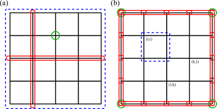
Figure 3: Panel (a): Schematic view of the $x$-th part of the reduced ground state subspace Hamiltonian $\tilde{H}_{x}$ (18): empty (green) circles are $\tilde{X}_{i,j}$ spin operators acting on every site, dashed (blue) frame symbolize nonlocal product of all $\tilde{X}_{i,j}$ operators products and solid (red) frames are products of $\tilde{X}_{i,j}$ along all lines and columns. Panel (b): Schematic view of $\tilde{H}_{z}$ (19): empty (green) circles in the corners stand for $\tilde{Z}_{i,j}$ spin operators related to the site $(i,j)$, solid (red) frames are $\tilde{Z}\tilde{Z}$ operator products acting on the boundaries of the lattice, and dashed (blue) square stands for one of the plaquette $\tilde{Z}\tilde{Z}\tilde{Z}\tilde{Z}$ spin operators. The exemplary three sites in the identity (21) are: $(i,i)$, $(k,l)$ and $(l,k)$.

Because of the PBC, all original $X_{i,j}$ spins are equivalent, so we choose $i=j$. The $x$-part (18) of the Hamiltonian is completely isotropic. Note that the $z$-part (19) would also be isotropic without the boundary terms (see Fig. 3); the effective Hamiltonian in the ground subspace has the symmetry of a square. Knowing that in the ground state we have only $Z_{2}$ degeneracy, one finds

$$\langle\tilde{X}_{i,i}\tilde{X}_{k,l}\rangle\equiv\langle\tilde{X}_{i,i}\tilde{X}_{l,k}\rangle,$$ (21)

for any $i$ and $(k,l)$. This proves the identity (16) for $\delta=0$; $\delta\neq 0$ case follows from lattice translations along rows.

The nontrivial consequences of Eq. (21) are: (i) hidden dimer order in the ground state of the QCM — dimer correlation functions in two a priori nonequivalent directions in the QCM are identical and robust for $X$-components for $\alpha<\frac{1}{2}$ (Fig. 4) and for $Z$-components for $\alpha>\frac{1}{2}$ (not shown), and (ii) long range two-site $\langle X_{i,j}X_{i+d+1,j}\rangle$ correlations along the columns which are equal to the multi-site $\langle XX\dots X\rangle$ correlations involving two neighboring rows, see Fig. 2(a). The latter comes from symmetry properties of the transformed Hamiltonian Eqs. (18) and (19) applied to the multi-site correlations:

$$\langle\tilde{X}_{i,i}\tilde{X}_{i,i+1}\dots\tilde{X}_{i,i+d}\rangle=\langle\tilde{X}_{i,i}\tilde{X}_{i+1,i}\dots\tilde{X}_{i+d,i}\rangle.$$ (22)

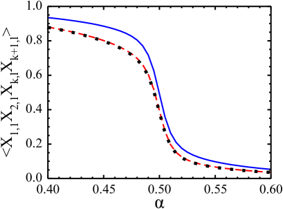
Figure 4: Dimer-dimer correlations $\langle X_{1,1}X_{2,1}X_{k,l}X_{k+1,l}\rangle$ for $L=6$ and $0.4<\alpha<0.6$: $(k,l)=(1,2)$, $(1,3)$ and $(1,4)$ are shown by solid, dashed and dotted line, respectively.

IV Numerical studies on finite square clusters

IV.1 Exact diagonalization methods

Although there is no exact solution for the 2D QCM Eq. (1), the latest Monte Carlo data Wenzel and Janke (2008) prove that the model exhibits a phase transition at finite temperature both in quantum and classical version, with symmetry breaking between $x$ and $z$ part of the QCM. In this section we suggests a scenario for a phase transition with increasing cluster size by the behavior of spin-spin correlation functions and von Neumann entropy of a single column in the ground state obtained via Lanczos algorithm. We also present the specific heat calculated using Kernel Polynomial Method (KPM).Weisse and Fehske (2008)

Ground state energies and energy gap of the 2D QCM has already been calculated for different values of $\alpha$ and for square $L\times L$ clusters with $L\in[2,5]$ using ED and for higher $L$ using Green’s function Monte Carlo method.Dorier et al. (2005) Our approach is based on Lanczos algorithm and KPM Weisse and Fehske (2008) which lets us calculate the densities of states and the partition functions for square lattices of the sizes up to $L=6$. We start by applying Lanczos algorithm to determine spectrum width which is needed for KPM calculations. The resulting few lowest energies that we get from the Lanczos recursion can be compared with the density of states to check whether the KPM results are correct.

One should be aware that the spectra of odd systems are qualitatively different from those of even ones. For the even systems operator $S$ defined as

$$S=\prod_{i,j=1}^{L}\frac{1}{2}\{1-(-1)^{i+j}\}Y_{i,j},$$ (23)

anticommutes with the Hamiltonian (1). This means that for every eigenvector $|v\rangle$ satisfying ${\cal H}(\alpha)|v\rangle=E(\alpha)|v\rangle$ we have another eigenvector $|w\rangle=S|v\rangle$ that satisfies ${\cal H}(\alpha)|w\rangle=-E(\alpha)|w\rangle$. This proves that for even values of $L$ spectrum of ${\cal H}(\alpha)$ is symmetric around zero but for odd $L$’s this property does not hold; then $S$ no longer anticommutes with the Hamiltonian. To obtain a symmetric spectrum in this case we would have to impose open boundary conditions. We would like to emphasize that both Lanczos and KPM calculation for $6\times 6$ lattice (with $2^{36}$-dimensional Hilbert space) would be nearly impossible without using the symmetry operators and reduced Hamiltonians given by Eqs. (7) and (8).

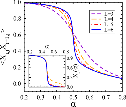
Figure 5: Nearest-neighbor spin correlations $\langle X_{i,j}X_{i+1,j}\rangle$ for different cluster sizes $L$ and long range correlations (inset) $X_{r}(\alpha)\equiv\langle X_{i,j}X_{i+r,j}\rangle$ for $L=6$ and $r=1,2,3$ shown with dashed (orange), long dashed (red) and solid (blue) lines, respectively.

IV.2 Ground state properties

In Fig. 5 we compare NN correlations $\langle X_{i,j}X_{i+1,j}\rangle$ as functions of $\alpha$ obtained via Lanczos algorithm for clusters of the sizes $L=3,4,5,6$. Curves for finite clusters converge to certain final functions with an infinite slope at $\alpha=\frac{1}{2}$ but not to a step function which would mean completely classical behavior. This result shows that even in the limit of large $L$ the 2D QCM preserves quantum correction even though it chooses to order in only one direction.Wenzel and Janke (2008) Looking at the inset of Fig. 5 we can see longer-range correlations of the form $X_{r}(\alpha)\equiv\langle X_{i,j}X_{i+r,j}\rangle$ (for symmetry reasons any other two-point correlation functions involving $X_{i,j}$ operators must be zero in the ground state) for the $L=6$ system and $r=1,2,3$. Their behavior is very similar to the NN correlations in the sector of $\alpha\leq\frac{1}{2}$ but for $\alpha>\frac{1}{2}$ they are strongly suppressed and effectively behave in a more classical way.

In Fig. 6(a) we show the ground state covariances of the bond operators $b_{i,j}^{x}\equiv X_{i,j}X_{i+1,j}$ and $b_{i,j}^{z}\equiv Z_{i,j}Z_{i,j+1}$, i.e.,

$${\cal C}(b_{i,j}^{x},b_{i,j}^{z})=\left\langle b_{i,j}^{x}b_{i,j}^{z}\right\rangle-\left\langle b_{i,j}^{x}\right\rangle\left\langle b_{i,j}^{z}\right\rangle.$$ (24)

Analogous covariances for whole $x$ and $z-$part of the Hamiltonian, namely $H^{x(z)}=\sum_{i,j}b_{i,j}^{x(z)}$, are shown in Fig. 6(b) as normalized by the total number of terms in $H^{x}H^{z}$, i.e., $L^{4}$. All covariances are of maximal magnitude at $\alpha=\frac{1}{2}$ and get suppressed when system size increases. In case of bond covariances suppression is not total and we have some finite covariance in whole range of $\alpha$ with cusp at $\alpha=\frac{1}{2}$, indicating singular behavior at this point. This means that locally vertical and horizontal bonds cannot be factorized despite the fact that the system chooses only one direction of ordering. On the other hand, the normalized nonlocal covariance of $H^{x}$ and $H^{z}$ tends to vanish for all $\alpha$ in the thermodynamic limit meaning that in the long-range vertical and horizontal bonds behave as independent from one another. We believe that this justifies the onset of directionally ordered phase for $L\to\infty$.

Figure 6: Local and nonlocal ground state covariances of: (a) the bond operators $b_{i,j}^{x}$ and $b_{i,j}^{z}$, and (b) the $x$ and $z-$part of the Hamiltonian, $H^{x}$ and $H^{z}$, normalized by $L^{4}$ for for different cluster sizes $L$ (note that the result for $L=3$ was scaled by factor $\frac{1}{5}$).

Another interesting quantity that can be calculated in the ground state is the von Neumann entropy of a chosen subsystem. This entropy tells us to what extent the full wave function of the system cannot be factorized and written as the wave function of the subsystem multiplied by the wave function of the rest. In case of the QCM on square lattice the most promising choice of a subsystem would be a single column or a single row of the square lattice. To calculate von Neumann entropy of a column we need to use its reduced density matrix $\rho_{L}$, defined as a partial trace of a full density matrix,

$$\rho=\left|\Psi_{0}\right\rangle\left\langle\Psi_{0}\right|,$$ (25)

taken over the spins outside the column. This definition, however true, is not very practical. For systems with spin $s=\frac{1}{2}$ one can derive a simpler formula:Eriksson and Johannesson (2009)

$$\rho_{L}=\frac{1}{2^{L}}\sum_{\mu_{1},..,\mu_{L}}\left\langle\sigma_{1}^{\mu_{1}}...\sigma_{L}^{\mu_{L}}\right\rangle\sigma_{1}^{\mu_{1}}...\sigma_{L}^{\mu_{L}}.$$ (26)

Here $\mu_{i}=0,x,y,z$, $\sigma_{i}^{0}=1$ and $\sigma_{i}^{\mu_{i}}$ are the spins taken from one column of a square cluster.

After diagonalizing $\rho_{L}$, which is of the size $2^{L}\times 2^{L}$, one can easily calculate von Neumann entropy as:

$${\cal S}_{L}=-\mathrm{Tr}\rho_{L}\log_{2}\rho_{L}.$$ (27)

For the symmetry reasons, described in detail in Sec. II, Eq. (26) simplifies greatly as only the $x$-component spin operators multiplied along the columns can give a finite average in the ground state and their number must be even. Thus, for $L\leq 6$ systems, the matrix $\rho_{L}$ can be constructed with two–point, four–point and single six–point correlation functions at most. Again, the reduced form of the compass Hamiltonian simplifies getting the ground state but we have to keep in mind that $\rho_{L}$ is expressed in terms of original spins.

The results of von Neumann entropy calculations for a column of length $L$ belonging to the $L\times L$ cluster is shown in Fig. 7(a). We can see that for $\alpha=0$ the entropy $S_{L}(\alpha)$ is finite as we expect from the product state. On the other hand, the system at $\alpha=0$ is purely classical and the Hamiltonian (1) describes a set of noninteracting Ising columns. Why is the ground state not a product of such columnar states? This is not visible for the present choice of basis adapted for the reduced form of the compass Hamiltonian given by Eqs. (7) and (8). Because of the spin transformations (4) and (5), the ground state from the subspace $r_{i}\equiv s_{i}\equiv 1$ found here is a superposition of two-column product states with equal weights and gives $S{\cal S}_{L}(0)=1$. This stays in agreement with the known fact that von Neumann entropy depends on the choice of basis and this dependence comes precisely from the partial trace of the density matrix $\rho$ Eq. (25). For that reason we should always employ the most natural basis for a given problem.

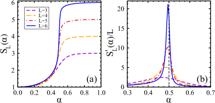
Figure 7: Panel (a) — von Neumann entropy ${\cal S}_{L}(\alpha)$ (27) of a column in the lattice of the size $L=3,4,5,6$ as a function of $\alpha$. Panel (b) — derivative of von Neumann entropy $S{\cal S}_{L}(\alpha)$ with respect to $\alpha$ normalized by $L$. The line character as in panel (a).

For $0<\alpha<1$ the subspace $r_{i}\equiv s_{i}\equiv 1$ is the most natural one because it is the only subspace with the ground state (up to global two–fold degeneracy). For $\alpha=0$ or $1$ the choice of the eigenbasis of $\sigma_{i}^{x}$ or $\sigma_{i}^{z}$ operators seems to be more natural one which implies ${\cal S}_{L}(0)={\cal S}_{L}(1)=0$ so the plot in Fig. 7(a) is valid only away from these points. The upper limit for ${\cal S}_{L}(\alpha)$ is always $L$ which can be easily proved by taking a state with all components equal. As we can see in Fig. 7(a) this limit is reached for $\alpha\to 1$ and before we have a region of abrupt change in ${\cal S}_{L}(\alpha)$ with slope growing with increasing size $L$. As a consequence, the derivative of ${\cal S}_{L}(\alpha)$ with respect to $\alpha$ normalized by $L$ increases with system size, see Fig. 7(b). Because of the above normalization the area under the plot is constant and equal to $1$. As we can see the curve tends to a delta function centered around $\alpha=\frac{1}{2}$ for growing system size $L$. This suggests that there is a quantum phase transition of the second order at $\alpha=\frac{1}{2}$ in the thermodynamic limit because second derivative of von Neumann entropy diverges, which stays in analogy to the classical entropy and classical phase transition.

We have also examined the overlap of the ground states obtained for $\alpha$ to the left and to the right of (before and after) the transition point at $\alpha=\frac{1}{2}$ called also a fidelity. In this case we are interested in fidelity $\chi_{L}(\alpha)$ defined as,

$$\chi_{L}(\alpha)\equiv\left\langle\psi_{0}(0^{+})\right.\left|\psi_{0}(\alpha)\right\rangle,$$ (28)

where $\left|\psi_{0}(\alpha)\right\rangle$ is a ground state for a given $\alpha$ and $\left|\psi_{0}(0^{+})\right\rangle$ is one of two possible $x$-ordered ground states for $\alpha$ being close to $0$. As we can see from Fig. 8(a), $\chi_{L}(\alpha)$ decays monotonously for growing $\alpha$ and the drop is most pronounced around $\alpha=\frac{1}{2}$, especially for few largest $L$, as one could expect. Less expected is that for small system sizes $\chi_{L}(\alpha)$ does not vanish at $\alpha=1$ though the $x$-order changes completely to the $z$-one. This effect is again due to the symmetries — the symmetry obeying ground state at $\alpha=0^{+}$ is a linear combination of the classical configurations found at $\alpha=0$ and hence not necessarily orthogonal to the one at $\alpha=1^{-}$. On the other hand, for growing system size these states become more and more orthogonal and already for $L=4$ we find that $\chi_{L}(\alpha)$ vanishes at $\alpha=1^{-}$.

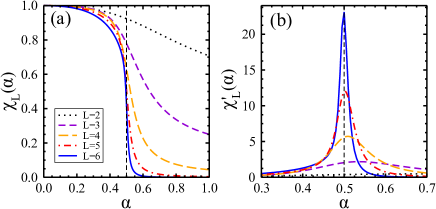
Figure 8: Panel (a) — fidelity $\chi_{L}(\alpha)$ (28) for different values of $L=2,\dots,6$. Panel (b) — derivative of the fidelity $\chi_{L}(\alpha)$ with respect to $\alpha$ for the same values of $\alpha$.

In the extreme case of $L=6$ system $\chi_{L}(\alpha)$ is strongly suppressed already at $\alpha=0.6$. Also in the $\alpha<\frac{1}{2}$ regime the fidelity drops faster for larger systems. The overall shape of the limiting $\chi_{L=6}(\alpha)$ curve is very similar to the one obtained with von Neumann entropy ${\cal S}_{L=6}(\alpha)$ of Fig. 7(a), especially below $\alpha=\frac{1}{2}$, showing the universality of the transition. Also the behaviors of the derivatives are qualitatively the same, see Figs. 8(b) and 7(b).

IV.3 The structure of energy levels for $L=6$

The discrete energy spectrum of the Ising model changes into a dense spectrum of the QCM when $\alpha$ increases, see Fig. 9, where we show the results of full brute-force ED of the $4\times 4$ periodic cluster (this task is impossible without using the symmetries of the QCM). All negative-energy levels for $0\leq\alpha\leq\frac{1}{2}$ are shown; full spectrum can be constructed from the plot in Fig. 9 by the mirror reflections with respect to $\alpha=\frac{1}{2}$ and $E_{n}=0$ axes. The structure of energy levels undergoes the evolution from the ladder-like classical excitation spectrum at $\alpha=0$ to the dense spectrum, with low-energy states separated by small gaps and a quasi-continuum structure at higher energy, at the isotropic point $\alpha=\frac{1}{2}$. Excited states at $\alpha=0$, being defected classical antiferromagnetic chains with energy determined by the number of spin defects, are well separated from one another until $\alpha\simeq 0.2$. For a fixed value of $\alpha$, increasing energy reflects increasing number of spin defects. The states with the lowest excitation energy, corresponding to a single spin defect, are less susceptible to the mixing caused by transverse terms in $H^{z}$, and remain separated from other states almost until the transition point at $\alpha=\frac{1}{2}$. Even at this point the mixing involves only singly and doubly defected states.

Figure 9: All the energy levels $E_{n}$ of the $L=4$ system as functions of $\alpha\in[0,\frac{1}{2}]$. The result is symmetric with respect to $E_{n}=0$ and $\alpha=\frac{1}{2}$ axes. [This figure is not reproduced here for technical reasons; it will appear in the published version of this paper.]

From the form of the QCM Hamiltonian (1), one can easily infer the relation between the slope of the energy level $E_{n}$ and the preferred ordering direction in the state $\left|\Psi_{n}\right\rangle$:

$$\frac{1}{J}\frac{d}{d\alpha}E_{n}(\alpha)=\left\langle\Psi_{n}(\alpha)\right|H^{x}-H^{z}\left|\Psi_{n}(\alpha)\right\rangle,$$ (29)

which means that states ordered by $H^{x}$ are related with energy levels with positive slope and the others are related with energy levels with negative slope. Zero slope indicates that the state has no preferred ordering direction; this happens to the ground state at $\alpha=\frac{1}{2}$ and the anticipated symmetry breaking between $H^{x}$ and $H^{z}$ implies that in the thermodynamic limit the lowest energy level will have a cusp at this point because any infinitesimal deviation from $\alpha=\frac{1}{2}$ must lead to strictly positive or negative slope of $E_{0}\left(\alpha=\frac{1}{2}\pm\varepsilon\right)$ (as also shown by the PEPS simulations of Ref. Orús et al., 2009).

Table 1 contains the two lowest energies, $E_{0}$ and $E_{1}$, from each of the $36$ nonequivalent invariant subspaces of the QCM for $L=6$ at $\alpha=\frac{1}{2}$. Their degeneracies $d$ agree with the considerations of Sec. III.1. Table 1 however was obtained by Lanczos recursions done in the full set of subspaces and then the energies were compared to arrange the subspaces into the classes. Similar Tables II-IV for the $L=2,3,4,5$ systems are presented in the Appendix A. Note that the $E_{0}$ energies appear in the ascending order and that $E_{0}$’s from the first $8$ subspaces form a multiplet of low lying states. This multiplet, already described in Ref. Dorier et al., 2005, consists of the classical ground state configurations at $\alpha=0$ and $\alpha=1$, split by the quantum corrections at $\alpha=\frac{1}{2}$. One could thus expect that the number of states in the multiplet is equal to $2\times 2^{L}$ but it turns out that the ground state of degeneracy $d=2$ is common for the two sets of states so the multiplicity equals to $2\times 2^{L}-2$. In case of the $L=6$ system this gives $126$ and can be obtained by adding the degeneracies of the first $8$ subspaces in Table 1. Looking at the results presented in the Appendix A, one can see that this holds for other system sizes as well.

Table 1: Ground state energy $E_{0}$ and first excited state energy $E_{1}$ (both in the units of $J$) and their degeneracies $d$ for $36$ nonequivalent subspaces of the $6\times 6$ QCM Eq. (1) at $\alpha=\frac{1}{2}$. States $n=1,\dots,8$ (bold face) come from the classical ground state manifolds at $\alpha=0,1$ and their total number is $126=2\left(2^{6}\right)-2$.

$n$	1	2	3	4	5	6
$E_{0}$	$-20.705$	$-20.547$	$-20.539$	$-20.537$	$-20.491$	$-20.489$
$E_{1}$	$-20.293$	$-19.734$	$-19.549$	$-19.462$	$-19.239$	$-19.147$
$d$	2	24	24	12	24	12
$n$	7	8	9	10	11	12
$E_{0}$	$-20.489$	$-20.451$	$-20.050$	$-19.984$	$-19.965$	$-19.877$
$E_{1}$	$-19.101$	$-18.910$	$-19.416$	$-19.359$	$-19.370$	$-19.521$
$d$	24	4	72	144	72	72
$n$	13	14	15	16	17	18
$E_{0}$	$-19.835$	$-19.834$	$-19.814$	$-19.813$	$-19.722$	$-19.707$
$E_{1}$	$-19.585$	$-19.158$	$-19.154$	$-19.140$	$-19.113$	$-19.012$
$d$	72	144	72	144	18	24
$n$	19	20	21	22	23	24
$E_{0}$	$-19.675$	$-19.627$	$-19.622$	$-19.611$	$-19.522$	$-19.461$
$E_{1}$	$-19.269$	$-19.292$	$-19.312$	$-19.276$	$-19.325$	$-19.096$
$d$	144	72	144	72	36	24
$n$	25	26	27	28	29	30
$E_{0}$	$-19.458$	$-19.39$	$-19.315$	$-19.304$	$-19.211$	$-19.207$
$E_{1}$	$-19.151$	$-18.869$	$-18.850$	$-18.880$	$-19.036$	$-18.741$
$d$	72	72	72	144	12	18
$n$	31	32	33	34	35	36
$E_{0}$	$-19.175$	$-19.073$	$-19.068$	$-18.900$	$-18.714$	$-18.264$
$E_{1}$	$-18.877$	$-18.689$	$-18.561$	$-18.429$	$-18.463$	$-17.918$
$d$	72	72	24	12	24	2

In Fig. 10 we show the extrapolation of different energies for the infinite system done using the data from Table 1 and from the Appendix. Fig. 10(a) shows the behavior of the ground state energy per site $\varepsilon_{0}$ as a function of $1/L^{2}$. As we can see the data points nicely lie on a straight line and the linear fit gives the extrapolated ground state energy per site equal to

$$\varepsilon_{0}(L\to\infty)=-(0.5575\pm 0.0007)J,$$ (30)

This value lies between the classical value of $\varepsilon_{0}^{\rm clas}=-0.5J$ which one can get by keeping only one part of the Hamiltonian, either $H^{x}$ or $H^{z}$, and a chain MF (CMF) value, $\varepsilon_{0}^{\rm CMF}\simeq-0.5661J$. The CMF approach that we used here relies on splitting the interaction along one direction and treating the system as a set of Ising chains in a transverse field coupled to the MF (see Ref. Brzezicki and Oleś, 2011 for more details). Such chains can be then solved exactly so the quantum physics within a single chain is well captured. Being variational, the CMF approach must give higher ground state energy than the exact ground state energy, and indeed the PEPS estimation for $\varepsilon_{0}$ is $\varepsilon_{0}^{\rm PEPS}\simeq-0.5684J$ (originally for different parametrization of interactions, see Ref. Orús et al., 2009), is only slightly lower than $\varepsilon_{0}^{\rm CMF}$. Therefore we can conclude that the linear extrapolation (30) is not fully satisfactory though all three energies lie indeed close to one another. Surprisingly, the CMF description of the 2D QCM turns out to be quite precise.

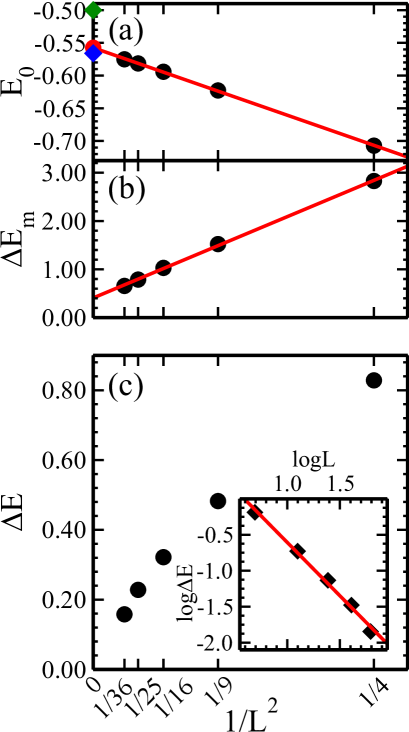
Figure 10: Extrapolations in $1/L^{2}$ for the $\alpha=\frac{1}{2}$ QCM. Filled circles represent: (a) the ground state energy $\varepsilon_{0}$ per site; (b) the gap $\Delta E_{m}$ between the ground state multiplet and the higher lying states; and (c) the energy gap $\Delta E$ to the first excited state. The (red) lines are the linear fits to the data for panels (a), (b). The inset of panel (c) shows the log-log plot for the energy gap $\Delta E$. The (red) dots at $1/L^{2}=0$ are the values predicted by the fits and square and diamond of panel (a) are the classical $\varepsilon_{0}^{\rm clas}$ and CMF $\varepsilon_{0}^{\rm CMF}$ extrapolated values of $\varepsilon_{0}$.

Fig. 10(b) depicts the energy gap $\Delta E_{m}$ between the ground state energy of the last subspace from the ground state multiplet and the lowest energy of the remaining subspaces. For instance, in case of the $L=6$ system the gap reads $\Delta E_{m}=E_{0}(n=9)-E_{0}(n=8)$. Like before, this quantity shows relatively good linear behavior as a function of $1/L^{2}$ (however small negative curvature can be observed for $L=6$) and the extrapolation in $L\to\infty$ can be easily performed to obtain $\Delta E_{m}(L\to\infty)=(0.408\pm 0.018)J$. The finite value of this gap for $L\to\infty$ means that the spectrum of the system divides into the low lying set of states separated by energy of $\Delta E_{m}$ from the rest. We argue that these states are the space of all possible nematic-ordered states and the finite value of $\Delta E_{m}$ makes the order robust at finite temperature up to $T_{c}=0.055J$ as shown in Ref. Wenzel and Janke, 2008. For the complete picture one could show that the width of the multiplet tends to zero for $L\to\infty$ but unfortunately its behavior as function of $1/L^{2}$ is quite irregular in this range of $L$.

Last but not least, we present the energy gap $\Delta E$ between the ground and the first excited state as a function of $1/L^{2}$ in Fig. 10(c). Note that this gap is a different quantity than the gaps discussed in Ref. Dorier et al., 2005 and is equivalent to the excitation energy associated with flipping one of the classical spins $\{r_{i},s_{i}\}$ of the reduced Hamiltonian of Eqs. (7) and (8). Surprisingly, it turns out that the gap does not decay exponentially with $L^{2}$ or $L$ (as it happens for the 1D transverse-field Ising model) but exhibits rather a power-law behavior. This can be seen more easily on a log-log plot in the inset of Fig. 10(c) where the data points show quite good linear behavior. The power-law fit of the form $\Delta E\propto(1/L^{2})^{1/\chi}$ gives critical exponent $\chi=1.418\pm 0.043$ which can be related to the dynamical critical exponent $z$ as $z=2/\chi$ (for the imaginary-time dynamical correlation length $\xi_{\tau}$ behaves like $\xi_{\tau}\propto 1/\Delta E$ and at the critical point $\xi_{\tau}\propto\xi^{z}$, see Ref. Park et al., 2010). Thus finally we obtain $z=1.409\pm 0.042$.

IV.4 Density of states and specific heat

The main benefit for ED calculations is that after the transformation the Hamiltonian of $L\times L$ compass model ($\alpha=\frac{1}{2}$) turns into $2^{2L-1}$ spin models, each one on an $(L-1)\times(L-1)$ lattice. In fact, the number of different models is much lower than $2^{2L-1}$; most of the resulting Hamiltonians differ only by a similarity transformation as shown in the Sec. III.1. For example, in case of the $6\times 6$ system we find out that only $36$ out of $2048$ Hamiltonians are different; their two lowest energies obtained using the Lanczos algorithm, and their degeneracies are given in Table 1. Similar data for lower system sizes can be found in the Appendix (in fact, these energies are known with much higher precision and up to $L=5$ we have determined all the high energy states).

Figure 11: Density of states $\rho(E)$ for the $6\times 6$ compass cluster at $\alpha=\frac{1}{2}$. Panel (a) — low energy region, lowest lying peaks agree with results of Lanczos recursion, excitation spectrum is discrete; panel (b) — full energy range in the logarithmic scale, parabolic behavior indicates dense gaussian spectrum of high-energy excitations.

This brings us to the calculation method — the KPM based on the expansion into the series of Chebyshev polynomials.Weisse and Fehske (2008) Chebyshev polynomial of the $n$-th degree is defined as $T_{n}(x)=\cos[n\arccos x]$ where $x\in[-1,1]$ and $n$ is integer. Further on, we are going to calculate $T_{n}$ of the Hamiltonian so first we need to renormalize it so that its spectrum fits into the interval $[-1,1]$. This can be done easily if we know the width of the spectrum. Our aim is to calculate the renormalized density of states $\tilde{\rho}(E)$ given by

$$\tilde{\rho}(E)=(1/D)\sum_{n=0}^{D-1}\delta(E-\tilde{E_{n}}),$$ (31)

where the sum is over eigenstates of ${\cal H}(\alpha)$ and $D$ is the dimension of the Hilbert space. The moments $\mu_{n}$ of the expansion of $\tilde{\rho}(E)$ in basis of Chebyshev polynomials can be expressed by:

$$\mu_{n}=\int_{-1}^{1}T_{n}(E)\tilde{\rho}(E)dE=\frac{1}{D}\textrm{Tr}\{T_{n}(\tilde{{\cal H}})\}\,.$$ (32)

Trace can be efficiently estimated using stochastic approximation:

$$\textrm{Tr}\,\{T_{n}(\tilde{{\cal H}})\}\approx\frac{1}{R}\sum_{r=1}^{R}\;\langle r|T_{n}(\tilde{{\cal H}})|r\rangle\,,$$ (33)

where $|r\rangle$ ($r=1,2,\dots,R$) are randomly picked complex vectors with components $\chi_{r,k}$ ($k=1,2,\dots,D$) satisfying $\langle\chi_{r,k}\rangle=0$, $\langle\chi_{r,k}\chi_{r^{\prime},l}\rangle=0$, $\langle\bar{\chi}_{r,k}\chi_{r^{\prime},l}\rangle=\delta_{r,r^{\prime}}\delta_{k,l}$ (the average is taken over the probability distribution). This approximation converges very rapidly to the true value of the trace, especially for a large value of $D$.

Action of the $T_{n}(\tilde{{\cal H}})$ operator on a vector $|r\rangle$ can be determined recursively using the following relation between Chebyshev polynomials:

$$T_{n}(\tilde{{\cal H}})|r\rangle=\{2\tilde{{\cal H}}\,T_{n-1}(\tilde{{\cal H}})-T_{n-2}(\tilde{{\cal H}})\}|r\rangle.$$ (34)

We can also use the relation

$$2T_{m}(x)T_{n}(x)=T_{m+n}(x)+T_{m-n}(x)$$ (35)

to get moments $\mu_{2n}$ from the polynomials of the degree $n$. Finally, the required function,

$$\tilde{\rho}(E)\approx\frac{1}{\pi\sqrt{1-E^{2}}}\left\{g_{0}\mu_{0}+2\sum_{n=1}^{N-1}g_{n}\mu_{n}T_{n}(E)\right\}\,,$$ (36)

can be reconstructed from the $N$ known moments, where coefficients $\{g_{n}\}$ come from the integral kernel we use for better convergence. Here we use Jackson kernel. Choosing the arguments of $\tilde{\rho}(E)$ as being equal to $E_{k}=\cos[(2k-1)\pi/2N^{\prime}]$ ($k=1,2,\dots,N^{\prime}$) we can change the last formula into a cosine Fourier series and use fast Fourier transform algorithms to obtain $\tilde{\rho}(E_{k})$ rapidly. This point is crucial when $N$ and $N^{\prime}$ are large, which is the case here; our choice will be $N=20000$ and $N^{\prime}=2N$. Using this procedure we can get the density of states for $L=4,5,6$ systems. After getting energy spectra for the nonequivalent subspaces we sum them with proper degeneracy factors to get the final density of states $\tilde{\rho}(E)$ and next the partition function via rescaling and numerical integration.

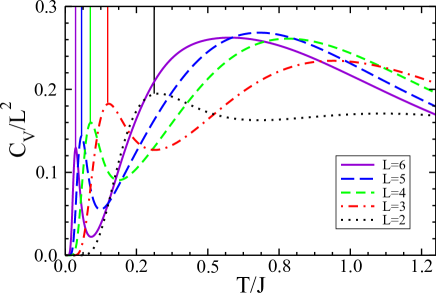
Figure 12: Specific heats $C_{V}/L^{2}$ per site as functions of temperature $T/J$ for $\alpha=\frac{1}{2}$ obtained for the QCM clusters of increasing size $L=2,\dots,6$. Vertical lines show the position of the low-energy peak in $C_{V}$ according to the canonical ensemble over the ground state multiplet only.

In Figs. 11(a) and 11(b) we display the density of states $\rho(E)$ (without normalization) for the system size $L=6$. Achieved resolution is such that one can distinguish single low-lying energy states and the positions of peaks agree with the results of Lanczos algorithm, see panel (a). In addition we get information about the degeneracy of energy levels encoded in the area below the peaks. This required very time-consuming calculations as the size of Hilbert space is above $30$ million. In Fig. 11(b) we present an overall view of full density of states in the logarithmic scale exhibiting gaussian behavior. Note different orders of magnitude in Figs. 11(a) and 11(b). Both plots show that in the thermodynamic limit the spectrum of the 2D QCM can be discrete in the lowest and highest-energy region and continuous in the center, which agrees with the existence of ordered phase above $T=0$.Wenzel and Janke (2008)

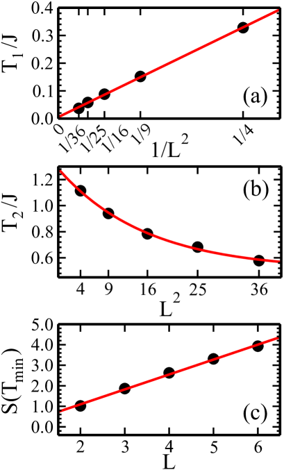
Figure 13: Finite-size extrapolations related with specific heat curves of Fig. 12: (a) — position $T_{1}$ of the low-temperature peak, (b) — position $T_{2}$ of the high-temperature peak, and (c) — entropy $S(T_{\rm min})$ at the temperature $T_{\rm min}$ of the dip between the two peaks in specific heat. Lines are the fits to the data points (filled circles).

In Fig. 12 we show the specific heat $C_{V}/L^{2}$ obtained for the compass $L\times L$ clusters calculated from: (i) the densities of states $\rho(E)$ for $L=5,6$, and (ii) the full energy spectrum for $L=2,3,4$. Additionally, to enhance the precision at low temperatures the lowest-lying energies obtained via stabilized Lanczos algorithm were used up to certain energy above $E_{0}$. For $L=5$ system all the energies up to $E\approx E_{0}+2J$ were determined by Lanczos algorithm but for $L=6$ only a few states above $E_{0}$ could be found due to the large size of the Hilbert space. The curves of specific heat of Fig. 12 exhibit two-peak structure similar to the one observed for a compass ladder (see Ref. Brzezicki and Oleś, 2010a), but in contrary to the ladder case the low-temperature peak seems to vanish for $L\to\infty$ and the specific heat develops a gap before the high-temperature peak.

On the other hand, we can see that the position of the low-temperature peak agrees well with multiplet structure of the low-lying energy levels described in Sec. IV.3 — one can calculate the partition function over them to obtain the low-energy specific heat, then we can determine the position of its peak and compare it with the plot of Fig. 12. As we can see the small peak coincides with the ground state multiplet peak for all values of $L$.

In Figs. 13(a) and 13(b) we show the positions $T_{1}$ and $T_{2}$ of the low- and high-temperature peaks as functions of $1/L^{2}$ and $L^{2}$, respectively. As we can see from its linear behavior $T_{1}$ scales as $1/L^{2}$ and its extrapolated value for $L\to\infty$ is zero. On the other hand, the linear fit for $T_{2}$ as function of $1/L^{2}$ turns out to be unsatisfactory and the best obtained fit is of the exponential form, with

$$T_{2}(L\to\infty)=(0.505\pm 0.035)J.$$ (37)

Finally, in Fig. 13(c) we show the scaling behavior of the entropy $S(T_{\rm min})$ calculated from the specific heat at the temperature $T_{\rm min}$ being the minimum between the two peaks in $C_{V}$ which separates the low- and the high-energy excitations of the model, see Fig. 12. As one could expect $S(T_{\rm min})$ scales linearly in $L$ because the number of the low-lying states is of the order of $2^{L}$ as shown in Section IV.3.

Effectively, the present data suggest that the specific heat curve in the thermodynamic limit would be rather like the one of classical Ising ladder (see Ref. Brzezicki and Oleś, 2010a), with a single broad peak in the high temperature regime and zero specific heat up to certain $T_{0}$, than the one of a compass ladder with robust low-energy excitations. This means that the thermal behavior of the 2D QCM is indeed mostly classical and agrees with the presence of ordered phase for finite $T$ in the thermodynamic limit.Wenzel and Janke (2008)

V Summary and conclusions

We have presented the consequences of symmetry properties of the 2D QCM which is in the center of interest at present.Nussinov and van den Brink (2013) Using this example we argue that for a certain class of pseudospin models, which have lower symmetry than SU(2), the spectral properties can be uniquely determined by discrete symmetries like parity. In the case of the conservation of spin parities in rows and columns in the 2D QCM (for $x$ and $z$-components of spins), we have observed that the ground state behaves according to a nonlocal Hamiltonian Eqs. (7) and (8). In the ground state most of the two-site spin correlations vanish and the two-dimer correlations exhibit the nontrivial hidden order. For a finite system, the low-energy excitations are the ground states of the QCM Hamiltonians in different invariant subspaces which, as shown for the $Q_{j}$ symmetries,Dorier et al. (2005) become degenerate with the ground state in the thermodynamic limit, leading to degeneracy $d$ being exponential in the linear system size $L$ ($d=2^{2L-1}$ or larger, if one could count the excited states from different subspaces). The invariant subspaces can be classified by lattice translations — the reduction of the Hilbert space achieved in this way is important for future numerical studies of the QCM and will play a role for spin models with similar symmetries.

The reduced QCM Hamiltonian turned out to be very useful for the state-of-the-art implementations of the ED techniques and gives the access to the system sizes unavailable otherwise. In contrast to the point-group or translational symmetries often explored for such models, spin transformations lead to spin Hamiltonian again which makes it particularly easy to implement. Although QCM has no sign problem and can be treated with powerful quantum Monte Carlo methods, ED gives most complete solution: the ground state wave function giving the access to all possible correlators and measures of entanglement. Using Lanczos and full diagonalization techniques we showed the behavior of all two-point correlation functions for different system sizes and the full structure of energy levels as functions of anisotropy parameter $\alpha$, indication of discrete-continuum nature of the spectrum of the QCM. Finally, we have obtained the ground state energy $\varepsilon_{0}$ per site up to $L=6$ and its extrapolation in the limit of $L\to\infty$, $\varepsilon_{0}(L\to\infty)=-(0.5575\pm 0.0007)J$, which is very close indeed to the CMF result, $\varepsilon_{0}^{\rm CMF}\approx-0.5661J$. Both values are also very close to the best estimate known from PEPS for the QCM,Orús et al. (2009) $\varepsilon_{0}^{\rm PEPS}\approx-0.5684J$.

The behavior of von Neumann entropy ${\cal S}_{L}(\alpha)$ of a single column of a square lattice together with the fidelity $\chi_{L}(\alpha)$ and the energy gap $\Delta E$ at $\alpha=\frac{1}{2}$, which decays in a power-low fashion for growing $L$, suggests that the phase transition at $\alpha=\frac{1}{2}$ is of the second order with dynamical critical exponent $z=1.409\pm 0.042$. On the other hand, there is strong evidence, provided by the PEPS simulations,Orús et al. (2009) that the transition is indeed of the first order. Following the idea of Ref. Eriksson and Johannesson, 2009 we argue that this discrepancy could be cured by adopting a similar scenario of a phase transition to the one suggested for the 1D QCM (see Ref. Eriksson and Johannesson, 2009) — $\alpha=\frac{1}{2}$ could be a multicritical point of a more general model whose special case is the isotropic QCM thus the transition carries the features of both first and second order.

Summarizing, using Kernel Polynomial Method we have gained the access to the full density of states function $\rho(E)$ for system sizes excluding full ED, i.e., for $L=5,6$. The obtained $\rho(E)$ for $L=6$ confirms that the spectrum consists of discrete states at low energy, accompanied by the continuum part at higher energy, as observed before for smaller system size ($L=4$).Dorier et al. (2005) In addition, the extrapolation of the gap $\Delta E_{m}$ in the limit $L\to\infty$ shows that the manifold of the low-lying states, which collapse to the degenerate ground state in the $L\to\infty$ limit,Dorier et al. (2005) develops a gap to the higher-lying states of the width $\Delta E_{m}=(0.408\pm 0.018)J$. This supports the existence of an ordered quasi-1D nematic phase at finite temperature.

It is quite remarkable that the specific heat of the system, calculated from $\rho(E)$ for growing $L$, evolves to the curve characteristic for a classical Ising ladder,Brzezicki and Oleś (2010a) with a single broad peak at $T_{2}=(0.505\pm 0.035)J$ and a gap in low temperature, as shown by the finite-size extrapolation. Within the error bar this is half of the classical excitation energy when only interactions along a single direction contribute. While the specific heat for a finite system consists of two characteristic peaks, we demonstrated a distinct behavior of these peaks: (i) the position of the broad peak at high temperature saturates exponentially with increasing system size $L^{2}$, and (ii) the low-temperature maximum decreases and its position approaches zero as $1/L^{2}$. Finally, the entropy related with the low-energy sector scales linearly with $L$ which agrees with the number of states in the low-energy manifold being of the order of $2^{L}$, as indicated beforeDorier et al. (2005) and confirmed by our analysis. This is another manifestation of a classical behavior of the QCM at finite temperature.

Appendix A Square clusters with $L<6$

As a supplement to Table 1 of Sec. IV.3, we present here analogous Tables with energies and degeneracies for inequivalent subspaces for other $L\times L$ clusters with $L<6$: Table 2 for $L=5$, Table 3 for $L=4$, and Table 4 for $L=3$ and for $L=2$.

Table 2: Ground state energy $E_{0}$ and first excited state energy $E_{1}$ (in the units of $J$) and their degeneracies $d$ for $10$ nonequivalent subspaces of the $5\times 5$ QCM Eq. (1) at $\alpha=\frac{1}{2}$. States $n=1,\dots,4$ (bold face) come from the classical ground state manifolds at $\alpha=0,1$ and their total number is $62=2\left(2^{5}\right)-2$.

$n$	1	2	3	4	5
$E_{0}$	$-14.54$	$-14.31$	$-14.30$	$-14.22$	$-13.75$
$E_{1}$	$-13.80$	$-13.15$	$-12.91$	$-12.50$	$-12.86$
$d$	2	20	20	20	50
$n$	6	7	8	9	10
$E_{0}$	$-13.67$	$-13.52$	$-13.45$	$-13.22$	$-12.79$
$E_{1}$	$-12.99$	$-13.26$	$-12.67$	$-12.88$	$-12.30$
$d$	100	50	100	100	50

Table 3: Ground state energy $E_{0}$ and first excited state energy $E_{1}$ (in the units of $J$) and their degeneracies $d$ for $10$ nonequivalent subspaces of the $4\times 4$ QCM Eq. (1) at $\alpha=1/2$. States $n=1,\dots,4$ (bold face) come from the classical ground state manifolds at $\alpha=0,1$ and their total number is $30=2\left(2^{4}\right)-2$.

$n$	1	2	3	4	5
$E_{0}$	$-9.51$	$-9.18$	$-9.17$	$-9.04$	$-8.48$
$E_{1}$	$-8.17$	$-7.32$	$-7.36$	$-6.76$	$-7.46$
$d$	2	16	8	4	32
$n$	6	7	8	9	10
$E_{0}$	$-8.38$	$-8.11$	$-8.05$	$-7.61$	$-6.84$
$E_{1}$	$-7.69$	$-6.98$	$-7.12$	$-7.33$	$-6.48$
$d$	32	8	16	8	2

Table 4: Ground state energy $E_{0}$ and first excited state energy $E_{1}$ (in the units of $J$) and their degeneracies $d$ for $3$ nonequivalent subspaces of the $3\times 3$ ($L=3$) and $2\times 2$ ($L=2$) QCM Eq. (1) at $\alpha=\frac{1}{2}$. States $n=1,2$ (bold face) come from the classical ground state manifolds at $\alpha=0,1$ and their total number is $2\left(2^{L}\right)-2$, i.e., 14 for $L=3$ and 6 for $L=2$.

		$L=3$			$L=2$
$n$	1	2	3	1	2	3
$E_{0}$	$-5.61$	$-5.12$	$-4.08$	$-2.83$	$-2.00$	$0.00$
$E_{1}$	$-3.00$	$-2.34$	$-3.20$	$+2.83$	$+2.00$	$0.00$
$d$	2	12	18	2	4	2

By comparing the data in Tables II-IV for different system size $L$, we observe that the total width of the spectrum increases with increasing $L$, but the first excitation energy $E_{1}-E_{0}$ decreases. It is also remarkable that the number of nonequivalent subspaces in the range of $L<6$ increases from odd $L$ to even $(L+1)$ but stays constant from an even $L$ to the next odd $(L+1)$ size. No general proof of this property could be found so far.

References

- Tokura and Nagaosa (2000) Y. Tokura and N. Nagaosa, Science 288, 462 (2000).
- Oleś et al. (2005) A. M. Oleś, G. Khaliullin, P. Horsch, and L. F. Feiner, Phys. Rev. B 72, 214431 (2005).
- Khaliullin (2005) G. Khaliullin, Prog. Theor. Phys. Suppl. 160 (2005).
- Oleś (2012) A. M. Oleś, J. Phys.: Condens. Matter 24, 313201 (2012).
- Feiner et al. (1997) L. F. Feiner, A. M. Oleś, and J. Zaanen, Phys. Rev. Lett. 78, 2799 (1997).
- Feiner et al. (1998) L. F. Feiner, A. M. Oleś, and J. Zaanen, J. Phys.: Condens. Matter 10, L555 (1998).
- Brzezicki et al. (2012) W. Brzezicki, J. Dziarmaga, and A. M. Oleś, Phys. Rev. Lett. 109, 237201 (2012).
- Brzezicki et al. (2013) W. Brzezicki, J. Dziarmaga, and A. M. Oleś, Phys. Rev. B 87, 064407 (2013).
- Feiner and Oleś (1999) L. F. Feiner and A. M. Oleś, Phys. Rev. B 59, 3295 (1999).
- Feiner and Oleś (2005) L. F. Feiner and A. M. Oleś, Phys. Rev. B 71, 144422 (2005).
- Khaliullin et al. (2001) G. Khaliullin, P. Horsch, and A. M. Oleś, Phys. Rev. Lett. 86, 3879 (2001).
- Horsch et al. (2008) P. Horsch, A. M. Oleś, L. F. Feiner, and G. Khaliullin, Phys. Rev. Lett. 100, 167205 (2008).
- Oleś et al. (2006) A. M. Oleś, P. Horsch, L. F. Feiner, and G. Khaliullin, Phys. Rev. Lett. 96, 147205 (2006).
- You (2012) W.-L. You, A. M. Oleś, and P. Horsch, Phys. Rev. B 86, 094412 (2012).
- van der Brink et al. (1999) J. van der Brink, P. Horsch, F. Mack, and A. M. Oleś, Phys. Rev. B 59, 6795 (1999).
- van den Brink (2004) J. van den Brink, New J. Phys. 6, 201 (2004).
- van Rynbach et al. (2010) A. van Rynbach, S. Todo, and S. Trebst, Phys. Rev. Lett. 105, 146402 (2010).
- Trousselet et al. (2012a) F. Trousselet, A. Ralko, and A. M. Oleś, Phys. Rev. B 86, 014432 (2012a).
- Nussinov and van den Brink (2013) Z. Nussinov and J. van den Brink, arXiv:1303.5922 (unpublished) (2013).
- Kugel and Khomskii (1982) K. I. Kugel and D. I. Khomskii, Sov. Phys. Usp. 25, 231 (1982) [Usp. Fiz. Nauk 136, 621 (1982)].
- Nussinov et al. (2004) Z. Nussinov, M. Biskup, L. Chayes, and J. van den Brink, Europhys. Lett. 67, 990 (2004).
- Nussinov and Fradkin (2005) Z. Nussinov and E. Fradkin, Phys. Rev. B 71, 195120 (2005).
- Xu and Moore (2004) C. Xu and J. E. Moore, Phys. Rev. Lett. 93, 047003 (2004).
- Vidal et al. (2009) J. Vidal, R. Thomale, K. P. Schmidt, and S. Dusuel, Phys. Rev. B 80, 081104 (2009).
- Cobanera et al. (2010) E. Cobanera, G. Ortiz, and Z. Nussinov, Phys. Rev. Lett. 104, 020402 (2010).
- Douçot et al. (2005) B. Douçot, M. V. Feigel’man, L. B. Ioffe, and A. S. Ioselevich, Phys. Rev. B 71, 024505 (2005).
- Gladchenko et al. (2009) S. Gladchenko, D. Olaya, E. Dupont-Ferrier, B. Douçot, L. B. Ioffe, and M. E. Gershenson, J. Phys. Soc. Jpn. 96, 1606 (2009).
- Milman et al. (2007) P. Milman, W. Maineult, S. Guibal, L. Guidoni, B. Douçot, L. Ioffe, and T. Coudreau, Phys. Rev. Lett. 99, 020503 (2007).
- Khomskii and Mostovoy (2003) D. I. Khomskii and M. V. Mostovoy, J. Phys. A: Math. Gen. 36, 9197 (2003).
- Dorier et al. (2005) J. Dorier, F. Becca, and F. Mila, Phys. Rev. B 72, 024448 (2005).
- You et al. (2010) W.-L. You, G.-S. Tian, and H.-Q. Lin, J. Phys. A: Math. Gen. 43, 275001 (2010).
- Chen et al. (2007) H.-D. Chen, C. Fang, J. Hu, and H. Yao, Phys. Rev. B 75, 144401 (2007).
- Orús et al. (2009) R. Orús, A. C. Doherty, and G. Vidal, Phys. Rev. Lett. 102, 077203 (2009).
- Wenzel and Janke (2008) S. Wenzel and W. Janke, Phys. Rev. B 78, 064402 (2008).
- Trousselet et al. (2010) F. Trousselet, A. M. Oleś, and P. Horsch, Europhys. Lett. 91, 40005 (2010).
- Trousselet et al. (2012b) F. Trousselet, A. M. Oleś, and P. Horsch, Phys. Rev. B 86, 134412 (2012b).
- Cincio et al. (2010) L. Cincio, J. Dziarmaga, and A. M. Oleś, Phys. Rev. B 82, 104416 (2010).
- Brzezicki et al. (2007) W. Brzezicki, J. Dziarmaga, and A. M. Oleś, Phys. Rev. B 75, 134415 (2007).
- Brzezicki and Oleś (2009a) W. Brzezicki and A. M. Oleś, Acta Phys. Pol. A 115, 162 (2009a).
- Perk et al. (1975) J. H. H. Perk, H. W. Capel, M. J. Zuilhof, and T. J. Siskens, Physica A 81, 319 (1975).
- Eriksson and Johannesson (2009) E. Eriksson and H. Johannesson, Phys. Rev. B 79, 224424 (2009).
- You and Tian (2008) W.-L. You and G.-S. Tian, Phys. Rev. B 78, 184406 (2008).
- Brzezicki and Oleś (2010a) W. Brzezicki and A. M. Oleś, Phys. Rev. B 82, 060401 (2010a).
- Brzezicki and Oleś (2010b) W. Brzezicki and A. M. Oleś, J. Phys.: Conf. Ser. 200, 012017 (2010b).
- Brzezicki (2011) W. Brzezicki, Lectures on the Physics of Strongly Correlated Systems XV, AIP Conference Proceedings, Vol. 1419 (AIP, New York, 2011) pp. 261-265.
- Nakano and Sakai (2011) H. Nakano and T. Sakai, J. Phys. Soc. Jpn. 80, 053704 (2011).
- Brzezicki and Oleś (2009b) W. Brzezicki and A. M. Oleś, Phys. Rev. B 80, 014405 (2009b).
- Brzezicki (2010) W. Brzezicki, Lectures on the Physics of Strongly Correlated Systems XIV, AIP Conference Proceedings, Vol. 1297 (AIP, New York, 2010) pp. 407-411.
- Weisse and Fehske (2008) A. Weisse and H. Fehske, Computational Many Particle Physics, Lect. Notes Phys., Vol. 739 (Springer, Berlin, 2008) pp. 545-577.
- Brzezicki and Oleś (2011) W. Brzezicki and A. M. Oleś, Phys. Rev. B 83, 214408 (2011).
- Park et al. (2010) T. Y. Park, Y. C. Lee, and J.-W. Lee, J. Korean Phys. Soc. 56, 1011 (2010).