Deformation Constraints on Solitons and D-branes

Abstract:

We derive a set of constraints on soliton solutions using geometric deformations, and transformations by internal symmetries with space-dependent parameters. We show that Derrick’s theorem and a more complete set of constraints due to Manton are special cases of these deformation constraints (DC). We demonstrate also that known soliton solutions obey the DC, and extract novel results by applying the constraints to systems of D-branes, taking into account both Dirac-Born-Infeld and Wess-Zumino actions, and examining cases with and without D-brane gauge fields. We also determine a relation with the Hamiltonian constraint for gravitational systems, and discuss configurations of finite extent, like Wilson lines.

1 Introduction

Solitons are defined as finite-energy static solutions to the classical equations of motion. They play an important role in a wide range of physical systems, from non-linear optics to particle physics. Famous examples include the kink solution in the sine-Gordon theory [1] and other integrable two-dimensional models, vortices of the Abelian-Higgs model [2, 3], magnetic monopoles [4, 5], skyrmions [6, 7] and many others.

In recent years, static solutions of D-branes, strings and gravitational actions have drawn increased interest. These solutions often have infinite energy, but in certain cases there soliton solutions do exist. One example is the dual description of a baryon in the Sakai-Sugimoto model, which is realized as an instanton on the D8 branes [8]. Both the “ old solitons” and those analyzed more recently are solutions of non-linear differential equations for which analytic solutions are very scarce. Conditions and constraints on such solutions serve as useful tools that guide one in selecting tractable ansätze or restricting the existence of solitonic states. The well-known Derrick-Hobart theorem [9, 10] is a prototypical example of such a constraint: it shows that scalar field theories with two derivatives can have soliton solutions only in one space dimension. More recently, Manton [11] developed an extended class of constraints for solitons. According to these conditions, the space integral of the stress tensor associated with static configurations must vanish for fields decaying sufficiently fast near the boundary of the space.

In [11] these conditions were applied to the Skyrme system, monopoles and vortices in Higgs models. Various aspects of Derrick’s theorem were also discussed in [12, 13, 14, 15, 16].

In this work we derive the constraints of [9, 10] and of [11] from a new perspective: infinitesimal geometrical deformations of solitons. Since a soliton is a stable solution to the equations of motion, it must lie at a minimum of the energy. If we deform the soliton by some small transformation, the deformed configuration’s energy must therefore be larger than the energy of the original soliton. This analysis yields conditions to be satisfied by any theory with soliton solutions, and can be used to impose constraints on these solutions.

First we study “geometrical” deformations around soliton solutions. We consider deformations which depend linearly on coordinates, like (nonisotropic) dilatations and shear transformations. We show that the former yield a generalization of Derrick’s theorem and the latter lead to Manton’s integral conditions.

A second class of deformations involves internal symmetries of the theory, which are broken by soliton solutions. In complete analogy with the “geometrical” constraints, we show that for energy-minimizing solitons, the volume integral of the space components of the conserved current is constrained. For systems with spontaneous breaking of the global symmetries, namely systems with Nambu-Goldstone bosons, the integral equals a finite surface term; otherwise, it must vanish. We refer to the constraints derived from both the geometrical and the internal symmetry deformations as “deformation constraints” (DC).

The bulk of this paper deals with the application of the DC to a wide class of models. We begin with a “warm-up:” generalizations of Derrick’s work to sigma models and higher derivative scalar actions. We then survey soliton systems in various dimensions and check that DC associated with conserved currents are fulfilled. These include (trivially) the topological currents, currents associated with global symmetries in the Skyrme model, and with local symmetries in the Abelian Higgs model and the ’t Hooft-Polyakov monopole [4, 5].

We then derive the DC for scaling deformations of the Dirac-Born-Infeld (DBI) action of D-branes, including both scalars and gauge fields on the brane: we write down the stress tensor of a general embedding, with electric and magnetic fields. We also introduce the Wess-Zumino (WZ) action, and compute the contributions to the stress tensor for the D1, D2 and D3 brane models. We then explore some specific examples of these systems.

Finally, we study properties of holographic MQCD[17]. For flavor M5-branes in an M-theory background we find that Derrick’s condition matches with the vanishing of the momentum density associated to a spatial direction. This relation is then realized in a general setup with scalar fields. Finally we show that for gravitational backgrounds this coincides with the “Hamiltonian constraint” derived by using the ADM formalism along the spatial direction.

The paper is organized as follows: in section §2 we describe deformations of static field configurations and deduce the DC. We consider first geometrical deformations (shears and anisotropic dilations), then deformations associated with internal symmetries. In section §3 we describe several applications of the DC to theories with soliton solutions. In §4 we apply these DC to D-branes and strings, including both the DBI and WZ actions. In section §5 we present some applications in string theory including flavor branes in M-theory, gravitational backgrounds, and Wilson lines. We summarize, conclude, and raise open questions in section §6. Two appendices contain details of known examples and small extensions: probe branes in brane backgrounds, D3-branes with electric and magnetic fields, and the DC in DBI theories with scalars.

2 Deformation constraints

Solitons need not be the lowest energy states available, but they must lie at minima of the energy – otherwise they can become locally unstable. From this simple statement one can derive a series of non-trivial constraints by slightly deforming the soliton solutions. In this work, we will study deformations of solitons under infinitesimal shears, dilatations, and internal symmetry transformations.

2.1 Geometrical deformations of solitons

Consider the simple case of a theory with one or more scalars $\phi^{a}$, that possesses a finite energy static solution, $\phi^{a}_{0}(x)$. How do small deformations affect the energy of this solution?

Generically, the energy of the soliton is a function of the fields and its derivatives,

$$E[\phi^{a}_{0}]=\int d^{d}x\,{\cal E}(\phi^{a}_{0},\partial_{i}\phi^{a}_{0})$$ (1)

where ${\cal E}$ is the energy density. Let’s say we deform the configuration by a geometric deformation in space, $\Lambda x$. The deform solution will look like

$$\phi^{a}_{\Lambda}(x)=\phi^{a}_{0}(\Lambda x).$$ (2)

For small deformations we can expand

$$(\Lambda x)^{i}\simeq x^{i}+\xi^{i}(x).$$ (3)

In what follows, we will consider only linear transformations of the form

$$(\Lambda x)^{i}=\Lambda^{i}_{\ j}x^{k}+b^{i}\simeq x^{i}+\lambda^{i}_{\ k}x^{k}+b^{i}.$$ (4)

These include rigid translations, $b^{i}$, rigid rotations when $\lambda^{i}_{\ j}$ is antisymmetric, anisotropic dilatations when $\lambda^{i}_{\ j}$ is diagonal, and volume-preserving shear deformations when $\lambda^{i}_{\ j}$ is symmetric and has no diagonal components. The underlying translational and rotational symmetry of the theory implies that the energy will not change under rigid translations and rotations, but it can change otherwise.

The energy of the configuration that has suffered a small deformation is, to leading order,

$$E[\phi^{a}_{\Lambda}] =\int d^{d}x\,{\cal E}\left(\phi^{a}_{\Lambda}(x),\partial_{i}\phi^{a}_{\Lambda}(x)\right)$$

$$=\int d^{d}x^{\prime}\left|\left|\frac{\delta x^{i}}{\delta{x^{j}}^{\prime}}\right|\right|{\cal E}\left(\phi^{a}_{0}(x^{\prime}),\frac{\partial{x^{j}}^{\prime}}{\partial x^{i}}\partial_{j}^{\prime}\phi^{a}_{0}(x^{\prime})\right)$$

$$\simeq\int d^{d}x^{\prime}{\cal E}\left(\phi_{0}^{a}(x^{\prime}),\partial_{i}\phi^{a}_{0}(x^{\prime})\right)+\int d^{d}x^{\prime}\,\partial_{i}\xi^{j}\left[\delta^{i}_{\ j}{\cal E}-\frac{\delta{\cal E}}{\delta\partial_{i}\phi^{a}}\partial_{j}\phi^{a}_{0}\right]$$

$$=E[\phi^{a}_{0}]-\int d^{d}x^{\prime}\,\partial_{i}\xi^{j}\Pi^{i}_{\ j}(\phi^{a}_{0}).$$ (5)

In the second line we have made the change of variables ${x^{i}}^{\prime}=(\Lambda x)^{i}$ and in the next lines we have expanded for $x^{i}\simeq{x^{i}}^{\prime}-\xi^{i}$. Here $\Pi^{i}_{\ j}$ is a stress tensor for static configurations, based on the energy density ${\cal E}$,

$$\Pi^{i}_{\ j}=\frac{\delta{\cal E}}{\delta\partial_{i}\phi^{a}}\partial_{j}\phi^{a}-\delta^{i}_{j}{\cal E}\leavevmode\nobreak\ .$$ (6)

The difference in the energy of the deformed solution compared to the original one is given by the stress tensor ($\Pi^{i}_{\ j}$) evaluated at the soliton solution:

$$E[\phi^{a}_{\Lambda}]-E[\phi^{a}_{0}]=\int d^{d}x\ \delta{\cal E}=-\int d^{d}x\,\partial_{i}\xi^{j}\Pi^{i}_{\ j}.$$ (7)

The variation of energy for a transformation linear in the coordinates becomes

$$E[\phi^{a}_{\Lambda}]-E[\phi^{a}_{0}]=-\lambda^{j}_{\ i}\int d^{d}x\,\Pi^{i}_{\ j},$$ (8)

If the integral on the right-hand-side (RHS) of (8) is non-vanishing, we can always choose $\lambda^{i}_{\ j}$ in such a way that the RHS becomes negative. This would mean that the transformed configuration is energetically favored over the original! For stable configurations, therefore, the integral should vanish:

$$\int d^{d}x\,\Pi^{i}_{\ j}=0.$$ (9)

This is automatically satisfied for static solutions to the equations of motion, up to boundary terms. The stability of static solutions would then be determined by the second order term, which should be positive if the soliton is a minimum energy solution.

The conditions (9) were first derived (in a different way) by Manton [11], where they were used to study monopoles, instantons, and Skyrmions. A linear combination of these conditions gives the vanishing of the trace of the stress tensor

$$\int d^{d}x\,\Pi^{i}_{\ i}=0.$$ (10)

This corresponds to an isotropic dilatation, the deformation used by Derrick to prove that no soliton solutions exist for $d>1$ in scalar theories with positive potentials [9, 10]. The proof, in essence, shows that $\Pi^{i}_{\ i}\geq 0$, so $\int\Pi^{i}_{\ i}=0$ only for the trivial solution. Physically (10) can be interpreted as the virial theorem for field theories (see e.g. [13, 18]). One can use (9) to impose more restrictive conditions on the field theory action or on the properties of the soliton solutions, as algebraic relations between derivatives of the fields and the potential.

It is important to note that in theories with only scalar fields, the energy density functional of a static configuration coincides with minus the Lagrangian density ${\cal E}=-{\cal L}$, and $\Pi^{i}_{\ j}$ coincides with minus the spatial part of the energy-momentum tensor

$$\Pi^{i}_{\ j}=-T^{i}_{\ j}=-\frac{\delta{\cal L}}{\delta\partial_{i}\phi^{a}}\partial_{j}\phi^{a}+\delta^{i}_{j}{\cal L}\leavevmode\nobreak\$$ (11)

This is not always the case, however. For instance, in gauge theories with electric fields turned on, the energy is a Legendre transform of the Lagrangian. Furthermore, the energy density functional is not unequivocally defined. It is identified with the time component of the energy-momentum tensor ${\cal E}=T^{0}_{\ 0}$, which can be modified by adding improvement terms. These terms do not affect the conservation equations but alter some properties of the energy-momentum tensor. For instance, in Maxwell’s theory the canonical energy-momentum tensor is not gauge invariant or positive definite: this can be fixed adding an improvement term. Generically,

$${\cal E}=T^{0}_{{\rm can}\,0}+\partial_{i}\Psi^{i0}_{\ \ 0},$$ (12)

where the improvement term $\Psi$ satisfies

$$\Psi^{\rho\mu}_{\ \ \nu}=-\Psi^{\mu\rho}_{\ \ \nu}.$$ (13)

This guarantees conservation of the (improved) energy-momentum tensor. For static configurations (that is, where the time derivatives of all fields vanish)

$${\cal E}=-{\cal L}+\partial_{i}\Psi^{i0}_{\ \ 0}.$$ (14)

Using the fact that $T^{i}_{\ j}=T^{i}_{{\rm can}\,j}+\partial_{k}\Psi^{ki}_{\ \ j}$ for static solutions, we find

$$\delta{\cal E}=-\partial_{i}\xi^{j}\Pi^{i}_{\ j}=\partial_{i}\xi^{j}T^{i}_{\ j}-\partial_{i}\left(\delta\Psi^{i0}_{\ \ 0}+\partial_{k}\Psi^{ki}_{\ \ j}\xi^{j}\right).$$ (15)

Choosing an appropriate energy density functional will be an important part of the analysis. We will keep the notation $\Pi^{i}_{\ j}$ to denote the stress tensor derived from the energy functional, to avoid confusion with the energy-momentum tensor (even in the cases where they are interchangeable).

The conditions (9) rely crucially on the fields dying off quickly at infinity. For a static solution, the conservation of the energy-momentum tensor implies that $\partial_{i}T^{i}_{\ j}=0$. It is then possible to express the variation as a surface term:

$$\int d^{d}x\,\partial_{i}\xi^{j}\Pi^{i}_{\ j} =\int d^{d}x\partial_{i}\left[-T^{i}_{\ j}\xi^{j}+\delta\Psi^{i0}_{\ \ 0}+\partial_{k}\Psi^{ki}_{\ \ j}\xi^{j}\right]$$

$$=\oint d^{d-1}\sigma_{i}\,\left[-T^{i}_{\ j}\xi^{j}+\delta\Psi^{i0}_{\ \ 0}+\partial_{k}\Psi^{ki}_{\ \ j}\xi^{j}\right],$$ (16)

which does not necessarily vanish for configurations that extremize the energy, because the transformations we use do not necessarily vanish at infinity. The transformations in such cases can thus affect the boundary conditions of the fields, if they fields so not die off sufficiently fast. Since it is the action together with the boundary conditions that defines the physical system, transformations that alter the boundary conditions relate two different physical systems, rather than comparing different field configurations within the same system. We will explain this issue in more detail when we discuss deformations of solitons by global symmetries in the next subsection.

2.2 BPS conditions and the stress tensor

Bogomolnyi-Prasad-Sommerfield (BPS) conditions [19, 20] are lower bounds on the energy of solutions to the equations of motion, as a function of their topological charge. They are very useful for finding soliton solutions, solutions that saturate the BPS bound can by found by solving a much simpler set of first order equations (rather than the second order equations of motion).

When a soliton saturates a BPS condition, not only the integral of the stress tensor (9), but the components of the stress tensor themselves vanish. It was argued in [21] that this can be understood as a consequence of supersymmetry, even in purely bosonic models. Consider for instance a scalar field $\phi$ in $1+1$ dimensions with a positive semi-definite potential. The supersymmetric extension of the theory is

$$S=\int d^{2}x\left(\frac{1}{2}\partial_{\mu}\phi\partial^{\mu}\phi+\frac{i}{2}\bar{\psi}\gamma^{\mu}\partial_{\mu}\psi+\frac{1}{2}F^{2}+FW(\phi)-\frac{1}{2}W^{\prime}(\phi)\bar{\psi}\psi\right)\,,$$ (17)

with $\psi$ a Majorana spinor and $F$ an auxiliary field. The spatial components of the stress tensor for a static bosonic configuration are

$$T_{01}=T_{10}=0,\ \ T_{11}=\frac{1}{2}(\partial_{1}\phi)^{2}-\frac{1}{2}W^{2}.$$ (18)

This coincides with the ordinary bosonic theory for the potential $V=W^{2}/2$.

Supersymmetry relates the components of the stress tensor to the components of the supercurrent

$$S_{\alpha}^{\mu}=(\gamma^{\nu}\partial_{\nu}\phi+iW)\gamma^{\mu}\psi,$$ (19)

through the supersymmetric Ward identity

$$\left\{S_{\alpha}^{\mu},\,\bar{Q}_{\beta}\right\}=2i\gamma^{\nu}T_{\nu}^{\ \mu}+2i{\gamma_{3}}_{\alpha\beta}W^{\prime}\epsilon^{\mu\nu}\partial_{\nu}\phi.$$ (20)

The last term is proportional to the topological current (whose time component integrates to the central charge). From this expression, one can use the fact that the BPS solution is invariant under half of the supercharges to show that the components of the stress tensor vanish. This was checked explicitly in [21] for $1+1$ dimensional scalars, and also for Abelian vortices in $2+1$ dimensions, but the argument can in principle be generalized to any supersymmetric theory with BPS soliton solutions.

2.3 Deformations by global symmetries

One can generalize the conditions (9) for geometrical deformations to deformation of global symmetries broken by the solitonic configuration. Consider a global symmetry with associated global conserved current $J^{\mu}$. For static solutions, current conservation implies $\partial_{i}J^{i}=0$. Following the same logic as before, we can deform the soliton solution $\phi^{a}(x)$ by a transformation

$$\delta_{\theta}\phi^{a}(x)=\theta^{A}(x){T_{A}}^{a}_{b}(\phi^{b}(x)),$$ (21)

where ${T_{A}}$ are generators of the symmetry group in the appropriate representation. The variation of the energy is

$$\delta_{\theta}E[\phi^{a}]=\int d^{d}x\,\left[\partial_{i}\theta^{A}J_{A}^{i}+\partial_{i}(\delta_{\theta}\Psi^{i0}_{\ \ 0})\right]=\int d^{d}x\,\partial_{i}\theta^{A}J_{A}^{i},$$ (22)

where for the moment we assume that the boundary integral vanishes. As before we can pick a transformation linear in the coordinates $\theta^{A}=C^{A}_{\ i}x^{i}$, and for arbitrary $C^{A}_{\ i}$ we find the conditions

$$\int d^{d}x\,J_{A}^{i}=0.$$ (23)

This condition should be satisfied by solutions to the equations of motion. For other configurations, there will be an instability such that the charges tend to rotate along the spatial directions.

It is easy to see, for instance, that (23) is trivially satisfied for topological currents in field theories, since the topological current associated with solitons of general dimension[22] is proportional to the Levi-Civita tensor. The space components of this current thus vanish for static configurations and (23) is simply zero, as discussed at greater length in section 3.3 below.

2.4 Boundary Terms

There is an important caveat that applies to both the conditions we have just derived for global internal symmetries and for geometrical deformations via the energy-momentum tensor. The variation of the energy has to vanish only up to a total derivative, but the conservation of the energy-momentum tensor and the current imply that the variations we study are total derivatives, as noted in (16) and via a similar identity for the current:

$$\int d^{d}x\partial_{i}\xi^{j}T^{i}_{\ j}=\oint d^{d-1}\sigma_{i}T^{i}_{\ j}\xi^{j}=\lim_{|x|\to\infty}\oint d^{d-1}x\hat{x}_{i}T^{i}_{\ j}\xi^{j},$$

$$\int d^{d}x\partial_{i}\theta^{A}J_{A}^{i}=\int d^{d}x\partial_{i}(\theta^{A}J^{i}_{A})=\oint d^{d-1}\sigma_{i}\theta^{A}J^{i}_{A}=\lim_{|x|\to\infty}\oint d^{d-1}x\hat{x}_{i}\theta^{A}J^{i}_{A}.$$ (24)

There are possible boundary contributions from the improvement terms as well. $\hat{x}^{i}$ is a unit vector along the $i$th spatial direction, and the surface integral is taken over a sphere whose radius goes to infinity. The integral over the energy-momentum tensor of the global currents does not need to vanish: it could also be a constant. This complication to (23) occurs because we have used transformations linear in the coordinates, $\xi^{i}=\lambda^{i}_{\ k}x^{k}$, $\theta^{A}=C^{A}_{k}x^{k}$, which introduce factors that diverge as the volume of the space

$$\oint d^{d-1}x\,x^{k}\sim|x|^{d}.$$ (25)

In order to have a finite integral, the conserved currents should decay as

$$\hat{x}_{i}T^{i}_{\ j}\sim\frac{1}{|x|^{d}},\ \ \hat{x}_{i}J_{A}^{i}\sim\frac{1}{|x|^{d}}.$$ (26)

For a global current, the conservation equation $\partial_{i}J_{A}^{i}=0$ implies that at leading order for large radii,

$$J_{A}^{i}=\frac{x^{2}\delta^{ij}-dx^{i}x^{j}}{|x|^{d+2}}v_{Aj}+\cdots,$$ (27)

where $v_{Aj}$ is some constant. In fact, $J_{A}^{i}$ itself is a total derivative

$$J_{A}^{i}=\partial^{i}\left(\frac{x^{j}v_{Aj}}{|x|^{d}}\right)=\partial^{i}\phi_{A},$$ (28)

and solving the conservation equation is equivalent to solving the equation for a massless scalar field $\partial^{i}\partial_{i}\phi_{A}=0$ when the solutions are static. For the energy-momentum tensor the situation is similar, except that the scalar will be labeled by a spatial index, $v_{Aj}\to v_{kj}$, $\phi_{A}\to\phi_{k}$.

The currents are proportional to the gradient of a scalar field when the associated symmetry has been spontaneously broken, and there are Goldstone bosons. From the argument above we see that the conditions (9) and (23) do not apply to those cases. The non-zero variation of the energy, in this case, is a consequence of changing the boundary conditions of the field configuration at infinity. For a Goldstone boson $\varphi^{A}$, a global symmetry transformation shifts the field

$$\varphi^{A}\to\varphi^{A}+\theta^{A}.$$ (29)

Since $\theta^{A}$ is linear in the coordinates, this modifies the asymptotic behavior of the field, so the deformation maps the original theory to a different physical system, not to a different point in the configuration space of the same system. The requirement of vanishing (or constant) integral for the stress tensor no longer yields a valid stability check for the soliton.

We have a similar problem if there are boundaries at a finite distance: linear deformations alter the boundary conditions, which will be reflected in the boundary contribution to the variation of the energy. One must then generalize the variational principle to include the boundaries in the analysis. This is particularly important for to the study open strings from the worldsheet perspective, or branes with boundaries.

3 Some applications in theories with soliton solutions

In this section we survey field theories that admit soliton solutions and analyze space integrals over the spatial components of the conserved currents. The latter include topological currents, currents associated with global symmetries and with local symmetries.

3.1 Derrick’s theorem

Derrick’s theorem is simply a consequence of (9), but we will often make use of isotropic scaling deformations according to Derrick’s original framework. In many cases, this already allows one to impose very strong constraints on possible soliton solutions, and in some cases, exclude them entirely. We review this strategy now, and point out some simple extensions to the original theorem. In Appendix A, we also apply isotropic scaling to the DBI action in some examples.

Consider the Lagrangian density of a scalar field in $d+1$ dimensions

$${\cal L}=-\frac{1}{2}\partial_{\mu}\phi\partial^{\mu}\phi-V(\phi),$$ (30)

where the potential is non-negative and vanishes at its minima. (We use the mainly plus metric convention.) The energy associated with this family of field configurations is

$$E=\int d^{d}x\left[\frac{1}{2}(\nabla\phi(\vec{x}))^{2}+V(\phi(\vec{x}))\right].$$ (31)

Let us consider a uniform scaling deformation of the soliton in this system: $\phi(x^{i})\rightarrow\phi(\lambda x^{i})$ for some positive real number, $\lambda$. The energy must be extremized on the stable solution: $dE(\lambda=1)/d\lambda=0$. Note that for the energy to actually be minimized we also need $d^{2}E/d\lambda^{2}>0$. The energy associated with this family of field configurations is

$$E(\lambda)=\int d^{d}x\left[\frac{1}{2}(\nabla\phi(\lambda\vec{x}))^{2}+V(\phi(\lambda\vec{x}))\right]=\lambda^{-d}\int d^{d}x\left[\frac{1}{2}\lambda^{2}(\nabla\phi(\vec{x}))^{2}+V(\phi(\vec{x}))\right],$$ (32)

where after performing the re-scaling of the soliton, we changed variables in the integral of the energy, $x^{\mu}\rightarrow x^{\mu}/\lambda$. The variation of the energy is thus

$$\left.\frac{dE(\lambda)}{d\lambda}\right|_{\lambda=1}=-\int d^{d}x\left[\frac{1}{2}(d-2)(\nabla\phi(\vec{x}))^{2}+dV(\phi(\vec{x}))\right]=0.$$ (33)

For $d>2$, each term must vanish separately. This occurs only for the vacuum state. For $d=2$, it is the potential alone which must vanish, but again this occurs only for the vacuum. Hence the statement of Derrick’s theorem: For $d\geq 2$ the only non-singular time independent solution of finite energy is the vacuum.

One can quickly derive a similar result for sigma models with Lagrangian

$${\cal L}=-\frac{1}{2}G^{ab}(\phi)\partial_{\mu}\phi_{a}\partial^{\mu}\phi_{b}-V(\phi_{a}).$$ (34)

Repeating the procedure of scaling $x\rightarrow\lambda x$ and demanding extremum for $\lambda=1$ one finds

$$\left.\frac{dE(\lambda)}{d\lambda}\right|_{\lambda=1}=-\int d^{d}x\left[\frac{1}{2}(d-2)G^{ab}\nabla\phi_{a}\nabla\phi_{b}+dV(\phi_{a})\right]=0\leavevmode\nobreak\ .$$ (35)

When the signature of the metric $G^{ab}(\phi)$ is positive then the conclusions for the generalized case are the same as for the flat space case; if the signature is not positive, (35) does not yield constraints in any dimension $d\neq 2$.

Higher derivative actions

Another interesting example is that of soliton solutions to differential equations with more than two derivatives, such as the KdV and non-linear Schrödinger equations. These can be derived as Euler-Lagrange equations of Lagrangians that include terms of higher than the first derivative of the field.

Let us discuss some theories of this type, which appear (and have been studied using Derrick’s theorem) in the context of galileons [15, 16]. First consider a Lagrangian that includes second order derivatives of scalar field

$${\cal L}=-\frac{1}{2}[(\partial_{\mu}\phi)^{2}+a(\partial_{\mu}\partial^{\mu}\phi)^{2}]-V(\phi)\leavevmode\nobreak\ .$$ (36)

The corresponding equation of motion reads

$$\partial_{\mu}\partial^{\mu}\phi-a\partial^{2}(\partial^{2}\phi)+\frac{\partial V(\phi)}{\partial\phi}=0\leavevmode\nobreak\ .$$ (37)

The action is invariant under space-time translations $x^{\mu}\rightarrow x^{\mu}+a^{\mu}$ and the corresponding conserved energy momentum tensor is given by

$$T_{\mu\nu}=\partial_{\mu}\phi\partial_{\nu}\phi+a[\partial^{2}\phi\partial_{\mu}\partial_{\nu}\phi-\partial_{\mu}(\partial^{2}\phi)\partial_{\nu}\phi]-\eta_{\mu\nu}{\cal L}.$$ (38)

For static configurations the Hamiltonian takes the form

$$H=\int d^{d}x\left[\frac{1}{2}(\nabla\phi)^{2}+\frac{1}{2}a(\nabla^{2}\phi)^{2}+V(\phi)\right].$$ (39)

Scaling $x\rightarrow\lambda x$ and requiring extremality for $\lambda=1$ we get

$$\left.\frac{dH}{d\lambda}\right|_{\lambda=1}=\int d^{d}x\left[\frac{1}{2}(2-d)(\nabla\phi)^{2}+\frac{1}{2}a(4-d)(\nabla^{2}\phi)^{2}-dV(\phi)\right].$$ (40)

The higher derivative terms thus ease the restriction on solitonic solutions for pure scalar field theories: we can get solitons for $d<4$.

Generalizing this result to any higher order derivative Lagrangian density, where the derivative terms are quadratic in the fields of the form

$${\cal L}=\frac{1}{2}[(\partial_{\mu}\phi)^{2}+\sum_{n}^{N}a_{n}(\partial^{n}\phi)^{2}]-V(\phi)],$$ (41)

one can see that the constraint in principle allows solitons for any dimension $d<2N$.

Monopoles

The conditions (9) can also be used to verify the existence of soliton solutions for systems involving gauge fields – these checks are performed in [11] for numerous examples; we present the analysis for monopoles.

To see how this works for gauge fields, consider a theory of a scalar plus gauge fields. The Lagrangian density is

$${\cal L}=-\frac{1}{4}F_{\mu\nu}F^{\mu\nu}-\frac{1}{2}(D_{\mu}\phi)^{*}(D^{\mu}\phi)-V(\phi^{*}\phi)$$ (42)

where $D_{\mu}=\partial_{\mu}-ieA_{\mu}$ The corresponding energy for static configurations ($F_{i0}=0$, $D_{0}\phi=0$) reads

$$E=\int d^{d}x\left[\frac{1}{4}F_{ij}F^{ij}+\frac{1}{2}(D_{i}\phi)^{*}(D^{i}\phi)+V(\phi^{*}\phi)\right]$$ (43)

For $d=3$ the stress tensor is

$$T_{ij}=F_{i}^{\ \mu}F_{j\mu}+\frac{1}{2}\left(D_{i}\phi^{*}D_{j}\phi+D_{j}\phi^{*}D_{i}\phi\right)-\delta_{ij}\left[\frac{1}{4}F_{kl}F^{kl}+\frac{1}{2}D_{k}\phi^{*}D^{k}\phi\right].$$ (44)

We examine the conditions (9), for real ($\phi=\phi^{*}$) configurations. Monopoles satisfy the Bogomolny equation $F_{ij}=\epsilon_{ijk}D_{k}\phi$, which implies

$$T_{ij}=(\delta_{ij}\delta_{kl}-\delta_{il}\delta_{kj})D_{k}\phi D_{l}\phi+D_{i}\phi D_{j}\phi-\delta_{ij}\left[\frac{1}{2}(D_{k}\phi)^{2}+\frac{1}{2}(D_{k}\phi)^{2}\right]=0.$$ (45)

We see that Manton’s conditions are satisfied trivially for monopole solutions, as we discussed above this is because they saturate a BPS condition.

3.2 Manton’s conditions and electrodynamics beyond Maxwell

It is interesting to consider Maxwellian electrodynamics in four flat dimensions, extended to include higher order terms. The DBI action is one example of such an action, but generically one can write some arbitrary Lagrangian ${\cal L}(X,Y)$ as a function of the two Lorentz-invariant combinations $X\equiv E^{2}-B^{2}$ and $Y\equiv{\vec{E}}\cdot{\vec{B}}$. Using $E_{i}=F_{0i}$ and $B_{i}=\frac{1}{2}\epsilon_{ilm}F_{lm}$, we can see that the energy density is given by

$${\cal E}=\frac{\delta{\cal L}}{\delta F_{0i}}F_{0i}-{\cal L}=2E^{2}\partial_{X}{\cal L}+Y\partial_{Y}{\cal L}-{\cal L}\leavevmode\nobreak\ .$$ (46)

The stress tensor then becomes

$$\Pi^{i}_{\phantom{i}j} =\frac{\delta{\cal E}}{\delta F_{0i}}F_{0j}+2\frac{\delta{\cal E}}{\delta F_{ik}}F_{jk}-{\cal E}\delta^{i}_{j}$$

$$=2\left(2E^{2}\partial_{X}^{2}{\cal L}+Y\partial_{X}\partial_{Y}{\cal L}+\partial_{X}{\cal L}\right)E_{i}E_{j}+2\left(2E^{2}\partial_{X}^{2}{\cal L}+Y\partial_{X}\partial_{Y}{\cal L}-\partial_{X}{\cal L}\right)B_{i}B_{j}$$

$$\quad+\left({\cal L}-2X\partial_{X}{\cal L}-Y\partial_{Y}{\cal L}+2XY\partial_{X}\partial_{Y}{\cal L}+Y^{2}\partial_{Y}^{2}{\cal L}-4E^{2}B^{2}\partial_{X}^{2}{\cal L}\right)\delta_{ij}\leavevmode\nobreak\ .$$ (47)

For Maxwell theory we have ${\cal L}=\frac{1}{2}X$, which gives

$$\Pi^{i}_{\phantom{i}j}=E_{i}E_{j}-B_{i}B_{j}-\frac{1}{2}\left(E^{2}-B^{2}\right)\delta_{ij}\leavevmode\nobreak\ .$$ (48)

$\Pi^{i}_{\ j}$ only vanishes for self-dual configurations $E_{i}=\pm B_{i}$. Together with the equations of motion, $\nabla\cdot\vec{E}=0$ and $\nabla\times\vec{B}=0$, one can see that there are indeed no regular self-dual finite-energy static solutions.

These results may be useful for constructing valid Lagrangian with soliton solutions. For instance, if we have a Lagrangian of the form ${\cal L}=Yf(X)$, the stress energy tensor becomes

$$\Pi^{i}_{\ j}=2\left(2E^{2}Yf^{\prime\prime}+2Yf^{\prime}\right)E_{i}E_{j}+4E^{2}Yf^{\prime\prime}B_{i}B_{j}-4E^{2}B^{2}Yf^{\prime\prime}\delta_{ij}\leavevmode\nobreak\ .$$ (49)

If one sets $E_{i}=0$, Manton’s conditions are satisfied for any $B_{i}$, so in principle one could have solitons constructed entirely from magnetic fields.

3.3 Restrictions on currents

Lorentz invariant theories that admit solitons have been thoroughly investigated. In this subsection we survey these theories, focusing on the space integrals of their conserved currents. We will check whether these integrals indeed vanish, or equal non-vanishing surface terms given by (2.4). We can classify the currents as (i) topological currents (ii) currents associated with global symmetries (iii) currents associated with local symmetries.

Topological currents

Topological currents are conserved without the use of equations of motion. Their general structure in $d$ space dimensions is of the form

$$J_{\mu}=\epsilon_{\mu\nu_{1}...\nu_{d}}\tilde{J}^{\nu_{1}...\nu_{d}}$$ (50)

where $\tilde{J}^{\nu_{1}...\nu_{d}}$ is a tensor of degree $d$ composed of the underlying fields and their derivatives.

Consider now the spatial components of the current. If $\tilde{J}^{\nu_{1}...\nu_{d}}$ is composed of scalar fields alone (be they Abelian or non-Abelian), it must include a time derivative. For static configurations the spatial components of the current vanish automatically. When the theory also includes gauge fields, for gauge-invariant topological currents we can choose the gauge $A_{0}=0$, and see that the spatial components of the current again vanish trivially. For completeness, we list here the topological current of various models.

• For the Sine-Gordon model [1], the current is $J_{\mu}=\epsilon_{\mu\nu}\partial^{\nu}\phi$ where $\phi$ is a scalar field.

• The baryon number in bosonized 1+1 dimensional QCD [23] is given by $J_{\mu}=\epsilon_{\mu\nu}Tr[g^{-1}\partial^{\nu}g]$ where $g\in U(N_{f})$ see the next subsection.

• In 3+1 dimensions the current of the non-Abelian $SU(2)$ magnetic monopole [4, 5] is $J_{\mu}=\epsilon_{\mu\nu\rho\sigma}\epsilon_{abc}\partial^{\nu}\phi^{a}\partial^{\rho}\phi^{b}\partial^{\sigma}\phi^{c}$ where $\phi^{a}$ is a scalar field in the adjoint representation of the group.

• For the Skyrme model [6], the current is $J_{\mu}=\frac{\epsilon_{\mu\nu\rho\sigma}}{24\pi^{2}}Tr[L^{\nu}L^{\rho}L^{\sigma}]$, where $L_{\mu}=u^{-1}\partial_{\mu}u$ and where $u$ is the Skyrme field.

• The topological current for the four-dimensional gauge instanton is $J_{\mu}=\frac{\epsilon_{\mu\nu\rho\sigma}}{16\pi^{2}}Tr[A^{\nu}\partial^{\rho}A^{\sigma}+\frac{2}{3}A_{\nu}A_{\rho}A_{\sigma}]$ where $A_{\mu}$ is the corresponding non-Abelian gauge field.

• In five-dimensional gauge theories, the topological current is given by $J=*F\wedge F$.

Global currents

Next we examine currents associated with global continuous symmetries in two cases where the key player is a scalar field, which is a group element (1) of the 1+1 dimensional bosonized multi-flavor QCD[23], and (2) of the Skyrme model in 3+1 dimensions [6].

1. Though the sine-Gordon model in 1+1 dimensions has no global conserved currents, its non-Abelian generalization, 1+1 dimensional bosonized multi-flavor QCD[23], does. In the strong coupling limit one can integrate over the color degrees of freedom, leaving a theory invariant under a $U(N_{f})$ global symmetry of the form

   $$S=N_{c}S_{WZW}(g)+m^{2}\int d^{2}x\operatorname{Tr\,}[g+g^{\dagger}]$$ (51)

   where $N_{c}$ is the number of colors, $S_{WZW}$ is the WZW action, $g$ is a group element $g\in U(N_{f})$. $m$ is a mass parameter which depends on the coupling and the quark mass, as given in [23]. This “mass term” is essential for the existence of stable soliton solutions, which describe the baryons of the theory. This is thus a 1+1 dimensional analog of the Skyrme model. The vector and axial flavor currents associated with the WZW action take the form

   $$J_{\mu}^{\frac{V}{A}}=\frac{iN_{c}}{8\pi}[(g^{-1}\partial_{\mu}g\pm g\partial_{\mu}g^{-1})+\epsilon_{\mu\nu}(g^{-1}\partial^{\nu}g\mp g\partial^{\nu}g^{-1})]\leavevmode\nobreak\ .$$ (52)

   For a static configuration the space component of the currents gets a contribution only from the first term. The classical soliton solution has the structure

   $$g_{0}(x)=\,{\rm diag}\,\left(1,...1,e^{-i\sqrt{\frac{4\pi}{N_{c}}}\varphi(x)}\right)$$ (53)

   where $\varphi(x)$ is a solution of the sine-Gordon equation $\partial_{x}^{2}\varphi-\mu^{2}\sin(\beta\varphi)=0$ with $\beta=\sqrt{\frac{4\pi}{N_{c}}}$ and $\mu^{2}=2\sqrt{\frac{4\pi}{N_{c}}}m^{2}$. It is straightforward to see that for this configuration the space component of the vector current vanishes. The spatial part of the axial current does not vanish: indeed, the second term in the action (51) is not invariant axial transformations.

2. In the four dimensional theory of “bosonized” baryons in the Skyrme model, integrals over the flavor currents are more interesting. The model of two flavors, without a mass term, is invariant under both the $SU(2)$ vector and axial flavor global symmetries. No mass term is needed to have soliton solutions, since the Skyrme term plays the role of stabilizing the solitons. The axial current is proportional to the first term of (52) plus higher derivative corrections from the Skyrme term. Recall that the two-flavor Skyrme model does not include a WZ term. Unlike the 1+1-d case, here the space components of the axial current do not vanish. The non-Abelian (axial) current was found in [7] to be

   $${J_{i}^{a}}=\frac{1}{4}F_{\pi}\frac{B}{r^{3}}[(\tau_{i}-3\vec{\tau}\cdot\hat{x}\hat{x}_{i})\tau^{a}]+...$$ (54)

   so that

   $$\int d^{3}x{J_{i}^{a}}=-\frac{2}{3}F_{\pi}^{3}B\pi\delta_{i}^{a}$$ (55)

   where $B=\frac{8.6}{e^{2}F_{\pi}^{2}}$ ($\frac{1}{32e^{2}}$ is the coefficient of the Skyrme term). Hence the volume integral of the space component of the axial current takes the form of (2.4), yielding the Skyrme model prediction for the axial coupling.

Currents associated with local symmetries

Let us now turn to gauge theories, which have conserved currents that follow from local symmetries. Gauge transformations leave the action invariant, so we perform transformations keeping the gauge fields fixed. For non-Abelian symmetries the current is not just conserved, but covariantly conserved. The variation of the energy is still a total derivative, however:

$$\delta_{\theta}E=\int d^{d}x\,D_{i}\theta^{A}J_{A}^{i}=\int d^{d}x\,\left[\partial_{i}\left(\theta^{A}J_{A}^{i}\right)-\theta^{A}D_{i}J_{A}^{i}\right]=\oint d^{d-1}\sigma\,n_{i}\theta^{A}J_{A}^{i}.$$ (56)

We discuss first the Abelian Higgs model [2, 3] and then the model of the $SU(2)$ non-Abelian magnetic monopole [4, 5]. In both two cases there are scalar fields that do not vanish at infinity, so the transformation we perform would in principle affect to the boundary conditions on the fields. However, it turns out that in these cases the constraints are also satisfied.

1. The Abelian Higgs model is defined by the following Lagrangian density

   $${\cal L}=-\frac{1}{4}F^{\mu\nu}F_{\mu\nu}+\frac{1}{2}|(\partial_{\mu}+ieA_{\mu})\phi|^{2}-c_{2}|\phi|^{2}-c_{4}(|\phi|^{2})^{2}$$ (57)

   where $\phi$ is a complex scalar field and $A_{\mu}$ is an Abelian gauge field. The corresponding equations of motion admit soliton solutions in the form of vortices [2]. The vortex has formally infinite energy because it is extended in the $z$ direction, but at each fixed value of $z$ the energy density per unit length is finite. We parameterize the complex scalar field and the gauge field in polar coordinates $\rho$ and $\varphi$ (there is no dependence on $z$) as

   $$\phi(\vec{x})=e^{-in\varphi}f(\rho)\qquad\vec{A}(\vec{x})=-\frac{A(\rho)}{\rho}\hat{\varphi},$$ (58)

   where $n$ is an integer. It was shown in [3] that for $c_{4}=e^{2}/8$ the soliton is BPS, hence the components of the stress tensor vanish $T_{\rho\rho}=T_{\varphi\varphi}=0$ and (9) is automatically satisfied. The model admits also an Abelian conserved current

   $$\vec{J}=i[\phi^{*}\vec{D}\phi-(\vec{D}\phi^{*})\phi]=2\left(n+A(\rho)\right)\frac{(f(\rho))^{2}}{\rho}\hat{\varphi}\leavevmode\nobreak\ .$$ (59)

   At large values of the radial coordinate $f$ and $A$ go to constants, $\lim_{\rho\rightarrow\infty}f(\rho)=\sqrt{\frac{c_{2}}{2c_{4}}}$ and $\lim_{\rho\rightarrow\infty}A(\rho)=-n$. The current indeed vanishes at infinity.

   We now examine the conditions (23) for a volume whose boundary is a cylinder of radius $\rho=R$ and with caps at $z=\pm L$. They take the form

   $$\int d^{3}x\partial_{i}(J^{i}\theta)=\lim_{R,L\to\infty}\oint d\varphi\left[\int_{-L}^{L}dz\left.\theta J_{\rho}\right|_{\rho=R}+\int_{0}^{R}\rho d\rho\left(\left.\theta J_{z}\right|_{z=L}-\left.\theta J_{z}\right|_{z=-L}\right)\right]=0\leavevmode\nobreak\ .$$ (60)

   These conditions are automatically satisfied as $J_{\rho}=J_{z}=0$.

2. We can also check the conditions (23) for the ’t Hooft-Polyakov[5, 4] monopole. The components of the stress tensor vanish because the BPS condition is saturated.

   The system includes $SO(3)$ gauge fields interacting with an iso-vector scalar field, with Lagrangian density

   $${\cal L}=-\frac{1}{4}F^{\mu\nu}_{a}F^{a}_{\mu\nu}+\frac{1}{2}D_{\mu}\vec{\phi}\cdot D^{\mu}\vec{\phi}-\frac{1}{4}\lambda(|\phi|^{2}-v^{2})^{2}$$ (61)

   where $a=1,2,3$. The current associated with the $SO(3)$ global symmetry is given by

   $$J^{a}_{\mu}=\epsilon^{a}_{bc}(D_{\mu}\phi)^{b}\phi^{c}\qquad(D_{\mu}\phi)^{a}=\partial_{\mu}\phi^{a}-e\epsilon^{a}_{bc}A_{\mu}^{b}\phi^{c}$$ (62)

   The corresponding equations of motion read

   $$(D_{\nu}F^{\nu\mu})^{a}=J_{\mu}^{a}\qquad(D^{\mu}D_{\mu}\phi)_{a}=-\lambda\phi^{a}(|\phi^{2}|-v^{2})^{2}$$ (63)

   The relevant ansatz for solutions of the scalar and gauge fields reads

   $$\phi^{a}(\vec{r})=H(evr)\frac{x^{a}}{er^{2}}\qquad A_{i}^{a}(\vec{x})=-\epsilon^{a}_{\ ij}\frac{x^{j}}{er^{2}}[1-K(evr)]$$ (64)

   where the functions $H$ and $K$, which are determined by solving the equations of motion, behave asymptotical as $H\sim evr$ and $K\sim evre^{-evr}$. Substituting the ansatz into the current we find

   $$J^{a}_{i}=\left(\frac{H(evr)}{er^{2}}\right)^{2}K(evr)\epsilon^{a}_{\ ij}x^{j}\leavevmode\nobreak\ .$$ (65)

   It is thus obvious that

   $$\int d^{3}xJ^{a}_{i}=\lim_{r\to\infty}\oint d\Omega_{2}\,x^{i}\hat{x}^{k}J^{a}_{k}=0$$ (66)

   in accordance with (23), as the projection of the current on the radial direction vanishes.

4 Conditions for brane and string actions

In the previous section, we illustrated the use of DC in known examples and some simple extensions. Even for these relatively simple models, finding solitonic solutions can be highly non-trivial, and is usually the result of a clever ansatz. For D-brane systems, in which the DBI action generates an infinite number of interaction terms, the task can be that much more difficult. The DC represent a relatively simple test which may exclude the existence of solitons in large classes of systems. While satisfying the DC is necessary but not sufficient for soliton solutions, they may also help to construct ansätze for new static solutions.

We note again that one should be careful when dealing with finite volume configurations, as the conditions we impose are based on transformations that generically do not leave boundary conditions invariant. As mentioned above, one can only compare the energies of configurations satisfying the same boundary conditions.

The low-energy dynamics of D$p$-branes in a weakly curved gravitational background are given by the Dirac-Born-Infeld (DBI) action,

$$S_{DBI}=-T_{p}\int d^{p+1}xe^{-\phi}\sqrt{-\det\left(g_{\mu\nu}+2\pi\alpha^{\prime}F_{\mu\nu}+B_{\mu\nu}\right)}.$$ (67)

$T_{p}$ is the $Dp$ brane tension, $\phi$ is the background dilaton field, $B_{\mu\nu}$ is the pullback of the bulk Neveu-Schwarz (NS) two-form, $F_{\mu\nu}$ is the field strength of the Abelian gauge field on the brane, and $g_{\mu\nu}$ is the pullback of the background metric to the brane worldvolume. In the following we will use Greek letters ($\mu,\nu,\dots$) to denote worldvolume coordinates and capital Latin letters ($M,N,\dots$) to denote bulk coordinates and indices. Later we will also use lower case Latin indices ($i,j,\dots)$ for the spatial coordinates on the brane worldvolume. The metric has Lorentzian signature and we continue to use a mostly plus convention. This action is valid only to leading order in an expansion involving gradients of the gauge field and higher curvature corrections to the background, with $\alpha^{\prime}$ setting the scale of the expansion.

D-branes also carry charges that couple to Ramond-Ramond (RR) forms, as described by the Wess-Zumino (WZ) action

$$S_{WZ}=T_{p}\int d^{p+1}x\sum_{k}C_{k}\wedge e^{2\pi\alpha^{\prime}F+B},$$ (68)

where $C_{k}$ is the pullback of the $k$-form RR potentials.

A very similar semiclassical description exists for fundamental strings, via the Nambu-Goto (NG) action:

$$S_{NG}=-\frac{1}{2\pi\alpha^{\prime}}\int d^{2}x\sqrt{-\det\left(g_{\mu\nu}\right)}.$$ (69)

The string is charged under the NS two-form, with a WZ action

$$S_{B}=\frac{1}{2\pi\alpha^{\prime}}\int d^{2}xB.$$ (70)

Given the similarity between D-brane effective actions and string actions, we can consider them within the same framework.

The branes’ embedding in a $D$-dimensional background is described by a set of scalars living on its worldvolume $X^{M}(x)$, $M=1,\cdots,D$. The scalars appear in the pullback of the metric,

$$g_{\mu\nu}=G_{MN}\partial_{\mu}X^{M}\partial_{\nu}X^{N},$$ (71)

where $G_{MN}$ is the metric of the background and can be a functional of the scalar fields $X^{M}$ when evaluated on the brane worldvolume. The DBI+WZ actions together constitute the action of a $p+1$-dimensional theory including the scalar fields $X^{M}$ and the gauge fields $F_{\mu\nu}$. For infinitely extended configurations, there should be no finite energy static configurations if there are no background forms, since nontrivial excitations of the worldvolume scalars increase the energy. Background forms, however, can act as chemical potentials that decrease the energy density of the branes. We can tune the potentials so that trivial configurations have zero energy, which for the simplest cases amounts to subtracting off the ground state energy, as one expects that the restriction on the existence of static soliton solutions still applies when the forms are turned off.

Before deriving Manton’s conditions in detail, we address a subtlety of these types of actions. The brane action is invariant under worldvolume diffeomorphisms, which naïvely would lead to empty conditions when one applies Derrick’s scaling of the coordinates. Let us illustrate this for the simplest case of the NG action. We assume that there is a static solution to the equations of motion $X^{M}(x)$, $\partial_{t}X^{M}=0$ and evaluate the energy for $X^{M}(\lambda x)$:

$$E(\lambda) =-S_{NG}=\frac{1}{2\pi\alpha^{\prime}}\int dtdx\sqrt{-G_{MN}\partial_{x}X^{M}(\lambda x)\partial_{x}X^{N}(\lambda x)}$$

$$=\frac{1}{2\pi\alpha^{\prime}}\int dtdx^{\prime}\lambda^{-1}\sqrt{-\lambda^{2}G_{MN}\partial_{x^{\prime}}X^{M}(x^{\prime})\partial_{x^{\prime}}X^{N}(x^{\prime})}=E(1).$$ (72)

In other words, the scaling is eliminated by the diffeomorphism invariance of the action. In order to find non-trivial conditions, we must gauge-fix the diffeomorphism invariance first. We will choose the standard static gauge everywhere, with the scalar fields $X^{M}$ split into those pointing along the worldvolume directions $X^{\mu}$ ($\mu=0,1,\dots,p$), and those pointing along the transverse directions $Y^{a}$ ($a=p+1,\dots,D-1$):

$$X^{\mu}(x)= \ x^{\mu}$$

$$X^{a}(x)= \ Y^{a}(x)$$ (73)

This choice may not be suitable for all possible situations, for instance if there are solutions that join two brane sheets by a throat [18, 24]. These will be multivalued in the static gauge and can evade the naïve constraints. We will ignore this issue in what follows.

We impose some other simplifying assumptions as well, which nevertheless include many physically interesting cases. We impose

• time and space translation invariance of the worldvolume action. This implies that the background metric, dilaton and RR forms will be independent of the directions along the brane.

• that the solutions be truly static, meaning that $\partial_{t}Y^{a}=0$. One could relax this condition keeping invariance under time translations of the action if $\partial_{t}Y^{a}$ is constant and the background metric is independent of $Y^{a}$.

Note that in order to apply the DC we need the energy to be a conserved quantity: time translation invariance is thus a necessary requirement. When we come to nontrivial gauge field configurations, we will include static electric fields, however. These are allowed because the actions we study are gauge invariant.

The outline of the rest of this section is as follows: first we study Derrick-type DC conditions on brane actions without gauge fields and WZ terms, then we derive the general form of the DC, including gauge fields; finally we apply the conditions to the lower dimensional cases (D1, D2 and D3) including also WZ terms, and consider some interesting examples.

4.1 Scaling constraints in brane actions with scalars

We start by assuming that there is a static solution to the equations of motion $Y^{a}(\{x^{i}\})$ depending only on the spatial coordinates, with no gauge fields turned on. The pullback of the metric in the static gauge is

$$g_{00}=G_{00},\ \ g_{0i}=G_{0i},\ \ g_{ij}=G_{ij}+G_{ab}\partial_{i}Y^{a}\partial_{j}Y^{b}.$$ (74)

Let us now evaluate the energy on some field configuration $Y^{a}(\{\lambda_{i}x^{i}\})$ (no summation). After re-scaling the spatial coordinates as $x^{i}\rightarrow\lambda^{i}x^{i}$ (no sum) we will have

$$E(\{\lambda_{i}\})=T_{p}\int d^{p}x\,e^{-\epsilon\phi}\left(\prod_{i=1}^{p}\lambda_{i}^{-1}\right)\left[\sqrt{-\det(g[\{\lambda_{i}\}]})-\sqrt{-\det G}\right].$$ (75)

For a D-brane $\epsilon=1$ and $T_{p}$ is the D-brane tension. For a string $\epsilon=0$, $p=1$ and $T_{p}$ is the string tension. The last term is due to a background form and is chosen such that for $\partial_{i}Y^{a}=0$ the energy is zero.

Derrick’s theorem does not explicitly forbid the existence of scalar-field solitonic solutions in the DBI action. If a static solution indeed exists and is stable, the energy should be stationary as a function of the $\lambda_{i}$:

$$0=\frac{dE}{d\lambda_{i}}=-T_{p}\int d^{p}x\,e^{-\epsilon\phi}\left(\sqrt{-\det g}-\sqrt{-\det G}-\sqrt{-\det g}\sum_{l}g^{il}(g_{il}-G_{il})\right)\leavevmode\nobreak\ ,$$ (76)

where we have used

$$\frac{dg_{kl}}{d\lambda_{i}}=2\delta_{k}^{i}\lambda_{l}G_{ab}\partial_{i}Y^{a}\partial_{l}Y^{b}=2\delta_{k}^{i}\lambda_{l}(g_{il}-G_{il}).$$ (77)

For the trivial configuration $g_{ij}=G_{ij}$, and Derrick’s conditions are clearly satisfied, but, as discussed in Appendix B, solitons cannot be excluded on general grounds. However, using conditions like (9) we can make concrete statements about some special cases.

Consider Dp-branes with arbitrary $p$, such that the pullback fields $Y^{a}$ depend only on a single coordinate, which we call $x$. Assuming $G_{0i}=0$, we can show that solitons of this type are not allowed from the DBI action alone. The regularized energy is given by

$$E=T_{p}\int d^{p}xe^{\epsilon\phi}\left[\sqrt{-\det g}-\sqrt{-\det G}\right]\leavevmode\nobreak\ ,$$ (78)

where for this simple case

$$\det g=\left(1+{G}^{xx}G_{ab}\partial_{x}Y^{a}\partial_{x}Y^{b}\right)\det G$$ (79)

so

$$E=T_{p}\int d^{p}xe^{\epsilon\phi}\left\{\sqrt{(-\det G)\left[1+{G}^{xx}G_{ab}\partial_{x}Y^{a}\partial_{x}Y^{b}\right]}-\sqrt{-\det G}\right\}\leavevmode\nobreak\ .$$ (80)

Taking $x\rightarrow\lambda x$ in the solution (and leaving the other coordinates fixed) we find

$$\left.\frac{dE}{d\lambda}\right|_{\lambda=1}=0=T_{p}\int d^{p}x\ \sqrt{\frac{-\det G}{1+{G}^{xx}G_{ab}\partial_{x}Y^{a}\partial_{x}Y^{b}}}\left\{\sqrt{1+{G}^{xx}G_{ab}\partial_{x}Y^{a}\partial_{x}Y^{b}}-1\right\}\leavevmode\nobreak\ .$$ (81)

For nontrivial $\partial_{x}Y^{a},$ the integrand must be greater than zero, and the condition (9) cannot be satisfied! Note that this is the case for any brane dimension, even $p=1$. We provide more detail for a particular example in §A.1.

4.2 DC in brane actions with scalars and gauge fields

We now consider the more complicated case of D-branes with gauge fields and scalars, deriving general conditions based on both scaling and shear deformations.

When electric fields are turned on, the energy is the Legendre transform of the Lagrangian,

$$E_{\rm can}=\int d^{p}x\,\frac{\delta S_{DBI}}{\delta\partial_{0}A_{i}}\partial_{0}A_{i}-S_{DBI}.$$ (82)

Since the DBI action is gauge invariant one can also write the energy as

$$E_{\rm can} =\int d^{p}x\,\frac{\delta S_{DBI}}{\delta F_{0i}}(F_{0i}+\partial_{i}A_{0})-S_{DBI}=\int d^{p+1}x\,\frac{\delta S_{DBI}}{\delta F_{0i}}F_{0i}-S_{DBI}$$

$$+\int d^{p+1}x\partial_{i}\left(A_{0}\frac{\delta S_{DBI}}{\delta F_{0i}}\right).$$ (83)

In the last term we have used Gauss’s law

$$\partial_{i}\left(\frac{\delta S_{DBI}}{\delta F_{0i}}\right)=0.$$ (84)

We can eliminate it by adding the improvement term

$$\Psi^{i0}_{\ \ 0}=-A_{0}\frac{\delta S_{DBI}}{\delta F_{0i}}.$$ (85)

Note that for static solutions $\partial_{0}\Psi^{0i}_{\ \ 0}=-\partial_{0}\Psi^{i0}_{\ \ 0}=0$, so the improvement term does not affect the $T^{i}_{\ 0}$ components of the energy-momentum tensor. The energy functional takes the expected gauge-invariant form

$$E_{DBI}=\int d^{p+1}x\,\frac{\delta S_{DBI}}{\delta F_{0i}}F_{0i}-S_{DBI}.$$ (86)

It will be convenient to write the argument of the square root factorizing the pullback of the metric from the gauge fields

$$g_{\mu\nu}+2\pi\alpha^{\prime}F_{\mu\nu}=g_{\alpha\nu}M_{\mu}^{\ \alpha},$$ (87)

where

$$M_{\mu}^{\phantom{\mu}\nu}=\delta_{\mu}^{\ \nu}+2\pi\alpha^{\prime}F_{\mu}^{\phantom{\mu}\nu}\leavevmode\nobreak\ .$$ (88)

The determinant factorizes as

$$\det\left(g_{\mu\nu}+2\pi\alpha^{\prime}F_{\mu\nu}\right)=\det g\,\det M.$$ (89)

To find the variation of $\det M$ with respect to the gauge fields we use the formula

$$\det M=\frac{1}{(p+1)!}\epsilon^{\mu_{1}\dots\mu_{p+1}}\epsilon_{\nu_{1}\dots\nu_{p+1}}M_{\mu_{1}}^{\phantom{\mu_{1}}\nu_{1}}M_{\mu_{2}}^{\phantom{\mu_{2}}\nu_{2}}\dots M_{\mu_{p+1}}^{\phantom{\mu_{p+1}}\nu_{p+1}}\leavevmode\nobreak\ ,$$ (90)

where the $\epsilon^{\mu_{1}\cdots\mu_{p+1}}=\epsilon_{\mu_{1}\cdots\mu_{p+1}}$ are Levi-Civita symbols. Then,

$$\frac{\delta S_{DBI}}{\delta F_{\mu\nu}}=-\frac{T_{p}}{2}e^{-\phi}\sqrt{\frac{-\det g}{\det M}}\frac{1}{p!}\epsilon^{\mu\mu_{2}\dots\mu_{p+1}}\epsilon_{\nu_{1}\dots\nu_{p+1}}(2\pi\alpha^{\prime})g^{\nu\nu_{1}}M_{\mu_{2}}^{\phantom{\mu_{2}}\nu_{2}}\dots M_{\mu_{p+1}}^{\phantom{\mu_{p+1}}\nu_{p+1}}\leavevmode\nobreak\ .$$ (91)

The energy becomes

$$E_{DBI}=T_{p}\int d^{p}xe^{-\phi}\sqrt{\frac{-\det g}{\det M}}\left[\det M-\frac{1}{2p!}\epsilon^{0\mu_{2}\dots\mu_{p+1}}\epsilon_{\nu_{1}\dots\nu_{p+1}}(M_{0}^{\ \nu_{1}}-\delta_{0}^{\ \nu_{1}})M_{\mu_{2}}^{\phantom{\mu_{2}}\nu_{2}}\dots M_{\mu_{p+1}}^{\phantom{\mu_{p+1}}\nu_{p+1}}\right]$$ (92)

Defining $\epsilon^{i_{1}\cdots i_{p}}=\epsilon^{0i_{1}\cdots i_{p}}$, we can further simplify this expression to

$$E_{DBI}=T_{p}\int d^{p}xe^{-\phi}\sqrt{\frac{-\det g}{\det M}}\left[\det M-\frac{1}{2}\left(\det M-\det\hat{M}\right)\right].$$ (93)

Following the notation of Appendix B, a hatted matrix only has indices in the spatial directions, so $\det\hat{M}=\det(M_{i}^{\ j})$. Finally, we can write the energy as

$$E_{DBI}=\frac{T_{p}}{2}\int d^{p}xe^{-\phi}\sqrt{-\det g\det M}\left[1+\frac{\det\hat{M}}{\det M}\right].$$ (94)

If the electric field is zero $\det M=\det\hat{M}$ and one recovers the result that the energy is minus the DBI action.

Assuming there exists some finite energy solution to the equations of motion, $(Y^{a}(\{x^{i}\}),F_{\mu\nu}(\{x^{i}\}))$, the energy should be stationary under deformations of the solution. A general infinitesimal deformation is characterized by a vector $\xi^{i}(x)$ linear in the coordinates. The deformed configurations are

$$Y^{a}(\{x^{i}+\xi^{i}\}),\ \ F^{\xi}_{\mu\nu}=F_{\mu\nu}(\{x^{i}+\xi^{i}\})+\partial_{\mu}\xi^{\alpha}F_{\alpha\nu}(\{x^{i}+\xi^{i}\})+\partial_{\nu}\xi^{\alpha}F_{\mu\alpha}(\{x^{i}+\xi^{i}\}).$$ (95)

In terms of electric and magnetic fields

$$F^{\xi}_{0i} =F_{0i}(\{x^{i}+\xi^{i}\})+\partial_{i}\xi^{j}F_{0j}(\{x^{i}+\xi^{i}\}),$$ (96)

$$F^{\xi}_{ij} =F_{ij}(\{x^{i}+\xi^{i}\})+\partial_{i}\xi^{k}F_{kj}(\{x^{i}+\xi^{i}\})+\partial_{j}\xi^{k}F_{ik}(\{x^{i}+\xi^{i}\}).$$ (97)

We introduce these expressions in the energy and perform a change of coordinates $x^{i}\to x^{i}-\xi^{i}(x)$. The change in the energy is

$$\delta_{\xi}E=\int d^{p}x\,\delta_{\xi}{\cal E}=-\int d^{p}x\,\Pi^{i}_{\ j}\partial_{i}\xi^{j},$$ (98)

where we have defined the stress tensor as

$$\Pi^{i}_{\ j}=\frac{\delta E_{DBI}}{\delta(\partial_{i}Y^{a})}\partial_{j}Y^{a}+\frac{\delta E_{DBI}}{\delta F_{0i}}F_{0j}+2\frac{\delta E_{DBI}}{\delta F_{ik}}F_{jk}-\delta^{i}_{\ j}{\cal E}.$$ (99)

We will now compute each term in this expression. We will use the fact that

$$\frac{\delta E_{DBI}}{\delta(\partial_{i}Y^{a})}=-\frac{\delta E_{DBI}}{\delta g^{\mu\nu}}g^{\mu\alpha}g^{\nu\beta}\frac{\delta g_{\alpha\beta}}{\delta(\partial_{i}Y^{a})}=-\frac{\delta E_{DBI}}{\delta g^{\mu\nu}}(g^{\mu k}g^{\nu i}+g^{\mu i}g^{\nu k})G_{ab}\partial_{k}Y^{b}.$$ (100)

We will compute the variation of $E_{DBI}$ with respect to the metric further down, but first consider the terms involving the gauge fields. In order to vary with respect to the electric field, note that $\det g$ is independent of $F_{0i}$, so the only contributions come from the variation of $\det M$ and $\det\hat{M}$. We can simplify the result by using

$$\frac{\delta}{\delta F_{0i}}\left(\frac{1}{\sqrt{\det M}}\right)=-\frac{1}{\det M}\frac{\delta\sqrt{\det M}}{\delta F_{0i}}.$$ (101)

Then, the variation of the energy is

$$\frac{\delta E_{DBI}}{\delta F_{0i}}=-\frac{1}{2}\frac{\delta S_{DBI}}{\delta F_{0i}}\left[1-\frac{\det\hat{M}}{\det M}\right]+\frac{T_{p}}{2}e^{-\phi}\sqrt{\frac{-\det g}{\det M}}\frac{\delta\det\hat{M}}{\delta F_{0i}}.$$ (102)

where the variation of the DBI action was given in formula (91). For the magnetic components the situation is similar,

$$\frac{\delta E_{DBI}}{\delta F_{ik}}=-\frac{1}{2}\frac{\delta S_{DBI}}{\delta F_{ik}}\left[1-\frac{\det\hat{M}}{\det M}\right]+\frac{T_{p}}{2}e^{-\phi}\sqrt{\frac{-\det g}{\det M}}\frac{\delta\det\hat{M}}{\delta F_{ik}}.$$ (103)

We will now compute the missing pieces, starting with the variation of the energy with respect to the metric

$$\frac{\delta E_{DBI}}{\delta g^{\mu\nu}}=-\frac{1}{2}{\cal E}g_{\mu\nu}+\frac{T_{p}}{4}e^{-\phi}\sqrt{\frac{-\det g}{\det M}}\left[1-\frac{\det\hat{M}}{\det M}\right]\frac{\delta\det M}{\delta g^{\mu\nu}}+\frac{T_{p}}{2}e^{-\phi}\sqrt{\frac{-\det g}{\det M}}\frac{\delta\det\hat{M}}{\delta g^{\mu\nu}}.$$ (104)

Note that $M$ depends on $F_{\mu}^{\ \nu}=g^{\nu\alpha}F_{\mu\alpha}$, then

$$\frac{\delta\det M}{\delta g^{\mu\nu}}=g_{\mu\beta}F_{\alpha\nu}\frac{\delta\det M}{\delta F_{\alpha\beta}}.$$ (105)

The same formulas can be used substituting $\det M$ by $\det\hat{M}$, since $\hat{M}$ depends on $F_{i}^{\ j}=g^{j\alpha}F_{i\alpha}$:

$$\frac{\delta\det\hat{M}}{\delta g^{\mu\nu}}=\frac{\delta\det\hat{M}}{\delta F_{i}^{\ j}}F_{i\nu}\delta^{\ j}_{\mu},\ \ \frac{\delta\det\hat{M}}{\delta F_{\alpha\beta}}=\frac{\delta\det\hat{M}}{\delta F_{i}^{\ j}}\delta^{\ \alpha}_{i}g^{\beta j}.$$ (106)

In order to simplify the expressions we will use the relation

$$\frac{T_{p}}{2}e^{-\phi}\sqrt{\frac{-\det g}{\det M}}\frac{\delta\det M}{\delta F_{\alpha\beta}}=-\frac{\delta S_{DBI}}{\delta F_{\alpha\beta}}.$$ (107)

Finally, adding all the terms we have the stress tensor

$$\Pi^{i}_{\ j} ={\cal E}_{DBI}\left(g^{ik}G_{ab}\partial_{k}Y^{a}\partial_{j}Y^{b}-\delta^{i}_{\ j}\right)+\delta^{i}_{j}{\cal E}_{DBI}^{0}$$ (108)

$$+\frac{1}{2}\left[\frac{\delta S_{DBI}}{\delta F_{0l}}\left[1-\frac{\det\hat{M}}{\det M}\right]+\frac{{\cal L}_{DBI}}{\det M}\frac{\delta\det\hat{M}}{\delta F_{0l}}\right]\left((F_{0}^{\ i}\delta_{l}^{k}+F_{0}^{\ k}\delta_{l}^{i})G_{ab}\partial_{k}Y^{a}\partial_{j}Y^{b}-\delta^{i}_{l}F_{0j}\right)$$

$$+\frac{1}{2}\left[\frac{\delta S_{DBI}}{\delta F_{nl}}\left[1-\frac{\det\hat{M}}{\det M}\right]+\frac{{\cal L}_{DBI}}{\det M}\frac{\delta\det\hat{M}}{\delta F_{nl}}\right]\left((F_{n}^{\ i}\delta_{l}^{k}+F_{n}^{\ k}\delta_{l}^{i})G_{ab}\partial_{k}Y^{a}\partial_{j}Y^{b}-2\delta^{i}_{n}F_{jl}\right)$$

where the index on $F_{i}^{l}$ in the above are raised using the pullback metric, $g$. In the first line of this expression we have included the term ${\cal E}_{DBI}^{0}\equiv{\cal E}_{DBI}(A_{\mu}=0,Y^{a}=0)$, the energy of the trivial configuration. This guarantees that the net energy density, ${\cal E}_{DBI}-{\cal E}_{DBI}^{0}$, is finite. When Ramond-Ramond fluxes are included in Dp-brane action, the integral of the $p$-form flux associated with the brane assumes on this role, so one must be careful not to double-count its contribution (for instance by always normalizing the trivial configuration to have zero energy).

Stress tensor for BPS configurations

As we discussed previously, solitons that saturate a BPS bound should have vanishing (spatial) stress tensor components. We check this now for a few examples.

Let us first examine the case where the gauge fields are turned off and $G_{0i}=0$. We find

$$\Pi^{i}_{\ j}={\cal E}_{DBI}(g^{ik}(g_{kj}-G_{kj})-\delta^{i}_{\ j})+\delta^{i}_{j}{\cal E}_{DBI}^{0}=\delta^{i}_{j}{\cal E}_{DBI}^{0}-{\cal E}_{DBI}g^{ik}G_{kj}.$$ (109)

It is easy to see that the components of the stress tensor vanish for the Abelian vortices constructed in [25]. The action is that of the M2 brane in flat space, which is the same as the $2+1$ dimensional DBI without the dilaton factor. We pick two directions along the brane, $x^{i}$ with $i=1,2$, and two directions transverse to the brane $Y^{1}=X$, $Y^{2}=Y$. We then impose the BPS condition

$$\partial_{i}X=\pm\epsilon_{ij}\partial_{j}Y.$$ (110)

In this simple case, if we factor out the tension of the M2 brane, ${\cal E}^{0}=1$, ${\cal E}=(1+(\partial Y)^{2})$ and $g_{ij}=(1+(\partial Y)^{2})\delta_{ij}$. Then,

$$\Pi^{i}_{\ j}=\delta^{i}_{j}-(1+(\partial Y)^{2})\frac{\delta^{ik}}{(1+(\partial Y)^{2})}\delta_{kj}=0.$$ (111)

Another example of a BPS configuration is an instanton in the D4-brane worldvolume. Here we allow magnetic but not electric fields or scalars to be turned on. Using $\det\hat{M}=\det M$, the components of the stress tensor (in units of the tension) become

$$\Pi^{i}_{\ j}=\delta^{i}_{j}(1-{\cal E}_{DBI})+\frac{{\cal E}_{DBI}}{\det\hat{M}}\frac{\delta\det\hat{M}}{\delta F_{ik}}F_{jk}.$$ (112)

When the (anti) self-duality condition $F_{ij}=\pm\frac{1}{2}\epsilon_{ijkl}F_{kl}$ is satisfied,

$$\frac{\delta\det\hat{M}}{\delta F_{ik}}=\sqrt{\det\hat{M}}F^{ik},$$ (113)

and the energy density becomes ${\cal E}_{DBI}=\sqrt{\det\hat{M}}=1+\frac{1}{4}F_{ij}F^{ij}$. Then,

$$\Pi^{i}_{\ j}=-\frac{1}{4}\delta^{i}_{j}F_{kl}F^{kl}+F^{ik}F_{jk}.$$ (114)

This is the stress tensor for Maxwell theory. We can also write it as

$$\Pi^{i}_{\ j}=\frac{1}{2}\left(F^{ik}-\frac{1}{2}\epsilon^{ikln}F_{ln}\right)\left(F_{jk}+\frac{1}{2}\epsilon_{jkln}F_{ln}\right)-\frac{1}{4}\left(\epsilon_{jkln}F^{ik}F^{ln}-\epsilon^{ikln}F_{jk}F_{ln}\right).$$ (115)

When the (anti) self-duality condition is satisfied it is easy to check that this vanishes exactly.

4.2.1 Adding Wess-Zumino terms

In order to make the energy of the brane finite, we can add an additional term from the WZ action which precisely cancels the energy density of trivial configurations. This term comes from the coupling of a Dp-brane to the RR $(p+1)$-form potential, and contains a variety of terms involving gauge fields as well:

$$S_{WZ}=T_{p}\int_{Dp}C_{p+1}=T_{p}\int d^{p+1}x\,\frac{1}{(p+1)!}\epsilon^{\alpha_{1}\cdots\alpha_{p+1}}C_{\mu_{1}\cdots\mu_{p+1}}\partial_{\alpha_{1}}X^{\mu_{1}}\cdots\partial_{\alpha_{p+1}}X^{\mu_{p+1}}.$$ (116)

To cancel the trivial configuration energy, we only need a $C_{p+1}$ that has support along the directions parallel to the brane, but we will allow more general coordinate dependence, and take into account the gauge-field-dependent terms in the WZ action as well.

Like the DBI action, the $C_{p+1}$ term is diffeomorphism invariant, so one must fix the gauge before deforming the solution. Then the pullback of the RR form potential is

$$S_{WZ}=T_{p}\int d^{p+1}x\,\sum_{n=0}^{p}\frac{1}{(p-1+n)!}\epsilon^{\mu_{1}\cdots\mu_{n}\alpha_{1}\cdots\alpha_{p+1-n}}C_{\mu_{1}\cdots\mu_{n}a_{1}\cdots a_{p+1-n}}\partial_{\alpha_{1}}Y^{a_{1}}\cdots\partial_{\alpha_{p+1}}Y^{a_{p+1-n}}.$$ (117)

Similar expressions can be found for terms involving gauge fields. We will now study the lower dimensional D-branes individually. We will assume throughout the calculation that $G_{ab}$ only depends on the transverse coordinates $Y^{a}$.

We will use the following notation: $C^{(k)}$ denotes the RR form potential of rank $k$. $\alpha^{\prime}$ factors are absorbed in the gauge fields $\tilde{F}_{MN}=2\pi\alpha^{\prime}F_{MN}$, and we sometimes use $B=\frac{1}{2}\epsilon^{ij}\tilde{F}_{ij}$ and $E_{i}=\tilde{F}_{0i}$ for magnetic and electric fields.

D1 brane

The Wess-Zumino action takes the simple form

$$S_{WZ,D1} =T_{1}\int d^{2}x\left[\frac{1}{2}\epsilon^{\mu\nu}C^{(2)}_{\mu\nu}+2\frac{1}{2}\epsilon^{\mu\alpha}C^{(2)}_{\mu a}\partial_{\alpha}Y^{a}+\frac{1}{2}\epsilon^{\alpha\beta}C^{(2)}_{ab}\partial_{\alpha}Y^{a}\partial_{\beta}Y^{b}+\frac{1}{2}C^{(0)}\epsilon^{\mu\nu}\tilde{F}_{\mu\nu}\right]$$

$$=T_{1}\int d^{2}x\left[C^{(2)}_{01}+C^{(2)}_{0a}\partial_{1}Y^{a}+C^{(0)}\tilde{F}_{01}\right],$$ (118)

Since we assume $\partial_{0}Y^{a}=0$, the term proportional to $\epsilon(\partial Y)^{2}$ vanishes.

The WZ contribution to the energy is

$$E_{WZ,D1}=-T_{1}\int dx\left[C^{(2)}_{01}+C^{(2)}_{0a}\partial_{1}Y^{a}+2\pi\alpha^{\prime}C^{(0)}F_{01}\right].$$ (119)

The first term should be such that when added to the contribution from the DBI part the total energy is finite $T_{1}C^{(2)}_{01}={\cal E}_{DBI}+\cdots$.

The contribution of the WZ terms to the stress tensor is

$$\Delta\Pi^{1}_{\ 1}=-T_{1}\left[C^{(2)}_{0a}\partial_{1}Y^{a}+2\pi\alpha^{\prime}C^{(0)}F_{01}\right]+T_{1}\left[C^{(2)}_{01}+C^{(2)}_{0a}\partial_{1}Y^{a}+2\pi\alpha^{\prime}C^{(0)}F_{01}\right]=T_{1}C^{(2)}_{01}.$$ (120)

So only the components of the $C_{2}$ RR potential along the directions of the D1 modify the DC. The stress tensor has only one component (we are assuming $G_{01}=0$):

$$\Pi^{1}_{\ 1}={\cal E}(g^{11}G_{ab}\partial_{1}Y^{a}\partial_{1}Y^{b}-1)+T_{1}C^{(2)}_{01}.$$ (121)

For a probe D1-brane in a background sourced by other parallel D1-branes, $T_{1}C^{(2)}_{01}={\cal E}$. If we also use that $G_{ab}\partial_{1}Y^{a}\partial_{1}Y^{b}=g_{11}-G_{11}$, then

$$\Pi^{1}_{\ 1}={\cal E}(1-g^{11}G_{11}).$$ (122)

Note that $g^{11}G_{11}=G_{11}/g_{11}\leq 1$, and $g^{11}G_{11}>0$. Therefore $\Pi^{1}_{\ 1}\geq 0$, being equal to zero only for the trivial configuration. For non-trivial configurations we would have

$$0<\int dx\,\Pi^{1}_{\ 1}.$$ (123)

In the absence of gauge fields there are no soliton solutions on the D1-brane, in agreement with our previous analysis.

D2 brane

For D2-branes the Wess-Zumino action is

$$S_{WZ,D2} =T_{2}\int d^{3}x\left[C^{(3)}_{012}+\epsilon^{ij}C^{(3)}_{0ia}\partial_{j}Y^{a}+\frac{1}{2}\epsilon^{ij}C^{(3)}_{0ab}\partial_{i}Y^{a}\partial_{j}Y^{b}\right.$$

$$\left.+\frac{1}{3}C^{(1)}_{0}B-\frac{1}{3}\epsilon^{ij}C^{(1)}_{i}E_{j}-\frac{1}{3}\epsilon^{ij}C^{(1)}_{a}\partial_{i}Y^{a}E_{j}\right],$$ (124)

From this expression we find the contribution to the energy

$$E_{WZ,D2} =\int d^{2}x\,{\cal E}_{WZ}=-T_{2}\int d^{2}x\left[C^{(3)}_{012}+\epsilon^{ij}C^{(3)}_{0ia}\partial_{j}Y^{a}+\frac{1}{2}\epsilon^{ij}C^{(3)}_{0ab}\partial_{i}Y^{a}\partial_{j}Y^{b}\right.$$

$$\left.+\frac{1}{3}C^{(1)}_{0}B-\frac{1}{3}\epsilon^{ij}\left(C^{(1)}_{i}+C^{(1)}_{a}\partial_{i}Y^{a}\right)E_{j}\right].$$ (125)

Again, the first term should be such that when added to the contribution from the DBI part the total energy is finite $T_{2}C^{(3)}_{012}={\cal E}_{DBI}+\cdots$.

The contribution of the WZ terms to the stress tensor is

$$\Delta\Pi^{i}_{\ j} =-T_{2}\left[\epsilon^{ki}C^{(3)}_{0ka}\partial_{j}Y^{a}+\epsilon^{ik}C^{(3)}_{0ab}\partial_{j}Y^{a}\partial_{k}Y^{b}+\frac{1}{3}C^{(1)}_{0}\epsilon^{ik}\tilde{F}_{jk}\right.$$

$$\left.-\frac{1}{3}\epsilon^{ki}\left(C^{(1)}_{k}+C^{(1)}_{a}\partial_{k}Y^{a}\right)E_{j}-\frac{1}{3}\epsilon^{ik}\left(C^{(1)}_{a}\partial_{j}Y^{a}\right)E_{k}\right]-\delta^{i}_{\ j}{\cal E}_{WZ}.$$ (126)

D3 brane

For D3 branes the Wess-Zumino action is

$$S_{WZ,D3} =T_{3}\int d^{4}x\left[C^{(4)}_{0123}+\frac{1}{2}\epsilon^{ijk}C^{(4)}_{0ajk}\partial_{i}Y^{a}+\frac{1}{2}\epsilon^{ijk}C^{(4)}_{0abk}\partial_{i}Y^{a}\partial_{j}Y^{b}\right.$$

$$\left.+\frac{1}{3!}\epsilon^{ijk}C^{(4)}_{0abc}\partial_{i}Y^{a}\partial_{j}Y^{b}\partial_{k}Y^{c}+\frac{1}{2\cdot 3!}\epsilon^{ijk}C^{(2)}_{0i}\tilde{F}_{jk}+\frac{1}{2\cdot 3!}\epsilon^{ijk}C^{(2)}_{0a}\partial_{i}Y^{a}\tilde{F}_{jk}\right.$$

$$\left.+\frac{1}{2\cdot 3!}\epsilon^{ijk}C^{(2)}_{ij}\tilde{F}_{0k}+\frac{1}{3!}\epsilon^{ijk}C^{(2)}_{ia}\partial_{j}Y^{a}\tilde{F}_{0k}+\frac{1}{2\cdot 3!}\epsilon^{ijk}C^{(2)}_{ab}\partial_{i}Y^{a}\partial_{j}Y^{b}\tilde{F}_{0k}+\frac{1}{2\cdot 3!}C^{(0)}\epsilon^{ijk}\tilde{F}_{0i}\tilde{F}_{jk}\right].$$ (127)

From this expression we find the contribution to the energy

$$E_{WZ,D3} =-T_{3}\int d^{3}x\left[C^{(4)}_{0123}+\frac{1}{2}\epsilon^{ijk}C^{(4)}_{0ajk}\partial_{i}Y^{a}+\frac{1}{2}\epsilon^{ijk}C^{(4)}_{0abk}\partial_{i}Y^{a}\partial_{j}Y^{b}\right.$$

$$\left.+\frac{1}{3!}\epsilon^{ijk}C^{(4)}_{0abc}\partial_{i}Y^{a}\partial_{j}Y^{b}\partial_{k}Y^{c}+\frac{1}{2\cdot 3!}\epsilon^{ijk}C^{(2)}_{0i}\tilde{F}_{jk}+\frac{1}{2\cdot 3!}\epsilon^{ijk}C^{(2)}_{0a}\partial_{i}Y^{a}\tilde{F}_{jk}\right.$$

$$\left.+\epsilon^{ijk}E_{k}\left(\frac{1}{2\cdot 3!}C^{(2)}_{ij}+\frac{1}{3!}C^{(2)}_{ia}\partial_{j}Y^{a}+\frac{1}{2\cdot 3!}C^{(2)}_{ab}\partial_{i}Y^{a}\partial_{j}Y^{b}+\frac{1}{2\cdot 3!}C^{(0)}\tilde{F}_{ij}\right)\right].$$ (128)

The first term should be such that when added to the contribution from the DBI part the total energy is finite $T_{3}C^{(4)}_{0123}={\cal E}_{DBI}+\cdots$.

The contribution of the WZ terms to the stress tensor is

$$\Delta\Pi^{i}_{\ j} =-T_{3}\left[\frac{1}{2}\epsilon^{ikl}C^{(4)}_{0akl}\partial_{j}Y^{a}+\epsilon^{ikl}C^{(4)}_{0abl}\partial_{j}Y^{a}\partial_{k}Y^{b}+\frac{1}{2}\epsilon^{ikl}C^{(4)}_{0abc}\partial_{j}Y^{a}\partial_{k}Y^{b}\partial_{l}Y^{c}\right.$$

$$\left.+\frac{1}{3!}\epsilon^{ikl}C^{(2)}_{0l}\tilde{F}_{jk}+\frac{1}{3!}\epsilon^{ikl}C^{(2)}_{0a}\partial_{l}Y^{a}\tilde{F}_{jk}+\frac{1}{2\cdot 3!}\epsilon^{ikl}C^{(2)}_{0a}\partial_{j}Y^{a}\tilde{F}_{kl}\right.$$

$$+\epsilon^{kli}E_{j}\left(\frac{1}{2\cdot 3!}C^{(2)}_{kl}+\frac{1}{3!}C^{(2)}_{la}\partial_{l}Y^{a}+\frac{1}{2\cdot 3!}C^{(2)}_{ab}\partial_{l}Y^{a}\partial_{l}Y^{b}+\frac{1}{2\cdot 3!}C^{(0)}\tilde{F}_{kl}\right)$$ (129)

$$\left.+\epsilon^{kil}E_{l}\left(\frac{1}{3!}C^{(2)}_{ka}\partial_{j}Y^{a}+\frac{1}{3!}C^{(2)}_{ab}\partial_{k}Y^{a}\partial_{j}Y^{b}-\frac{1}{3!}C^{(0)}\tilde{F}_{jk}\right)\right]-\delta^{i}_{\ j}{\cal E}_{WZ}.$$ (130)

4.2.2 Examples in flat space

D1 brane with electric field

We consider a D1 brane in some background, described by a DBI action and Chern-Simons action. The vanishing of the stress tensor imposes the condition

$$0= 2C^{(2)}_{01}-\frac{e^{-\phi}G_{00}G_{11}}{(-G_{00}g_{11}-\tilde{F}_{01}^{2})^{3/2}}\left(2\tilde{F}_{01}^{2}+G_{00}g_{11}\right)\leavevmode\nobreak\ .$$ (131)

Strictly speaking we need to impose only that the integral of the stress tensor vanishes, if this condition can be satisfied there could be BPS solitons. If we allow electric fields ${\tilde{E}}=\tilde{F}_{01}$ and $Y^{\prime}$ but remain in a flat background we have

$$0=2C_{01}-e^{-\phi}\frac{1+Y^{\prime 2}-2{\tilde{E}}^{2}}{(1+Y^{\prime 2}-{\tilde{E}}^{2})^{3/2}}\leavevmode\nobreak\ .$$ (132)

We know (already from the action, in fact) that we must have ${\tilde{E}}^{2}<1+Y^{\prime 2}$. Let’s assume no backreaction of the probe on the dilaton or the background, and take $2C_{01}=e^{-\phi}$ . This implies

$$0=\ 2C_{01}\left\{1-\frac{1+Y^{\prime 2}-2{\tilde{E}}^{2}}{(1+Y^{\prime 2}-{\tilde{E}}^{2})^{3/2}}\right\}\leavevmode\nobreak\ .$$ (133)

The solution must also satisfy equations of motion. Since these have no direct dependence on $x^{1}$, we can write them in terms of integrals of motion,

$$\frac{Y^{\prime}}{\sqrt{1+Y^{\prime 2}-{\tilde{E}}^{2}}}= e^{\phi}Q_{Y}$$ (134)

$$-\frac{{\tilde{E}}}{\sqrt{1+Y^{\prime 2}-{\tilde{E}}^{2}}}= e^{\phi}Q_{F}$$ (135)

where $Q_{Y}$ and $Q_{F}$ are constants. Adding and subtracting these we have

$$\frac{(Y^{\prime}-{\tilde{E}})}{\sqrt{1+Y^{\prime 2}-{\tilde{E}}^{2}}} =e^{\phi}(Q_{Y}+Q_{F})\qquad\qquad\frac{(Y^{\prime}+{\tilde{E}})}{\sqrt{1+Y^{\prime 2}-{\tilde{E}}^{2}}}=e^{\phi}(Q_{Y}-Q_{F})$$

$$\Rightarrow \frac{(Y^{\prime 2}-{\tilde{E}}^{2})}{1+Y^{\prime 2}-{\tilde{E}}^{2}}=e^{2\phi}(Q_{Y}^{2}-Q_{F}^{2})\equiv Q^{2}(x)$$ (137)

where in the second line we multiplied the two equations together. We can simplify this to give

$$Y^{\prime 2}-{\tilde{E}}^{2}=\frac{Q^{2}}{1-Q^{2}}\leavevmode\nobreak\ .$$ (138)

Using this result we can simplify the Derrick-type condition of equation (132):

$$0=e^{-\phi}\left\{1-\sqrt{1-Q^{2}}\left[1-(1-Q^{2}){\tilde{E}}^{2}\right]\right\}\leavevmode\nobreak\ .$$ (139)

This gives

$${\tilde{E}}^{2} =-(1-Q^{2})^{-3/2}\left(1-\sqrt{1-Q^{2}}\right)$$ (140)

This would require ${\tilde{E}}^{2}<0$: a contradiction. We can now see that on the D1-branes, there are no BPS solitons.

D2 brane with magnetic field

In §4.2 we considered BPS Abelian vortices. We will see now that when a magnetic field is turned on in the D-brane action, such configurations cannot exist. We restrict to $E_{i}=0$, we also require $C^{(3)}_{012}=e^{-\phi}$ in order to have finite energy configurations, and take the same duality condition for scalar fields as before (110). The induced metric and DBI energy density are

$$g_{ij}=(1+(\partial Y)^{2})\delta_{ij},\ \ {\cal E}_{DBI}=\sqrt{(1+(\partial Y)^{2})^{2}+B^{2}}.$$ (141)

We will also need

$$\det M=\det\hat{M}=1+\frac{B^{2}}{(1+(\partial Y)^{2})^{2}}.$$ (142)

The contribution from the magnetic fields to the stress tensor (108) is

$${\Pi_{B}}^{i}_{\ j}=\frac{1}{2}\frac{{\cal L}_{DBI}}{\det\hat{M}}\frac{\delta\det\hat{M}}{\delta F_{nl}}\left((F_{n}^{\ i}\delta_{l}^{k}+F_{n}^{\ k}\delta_{l}^{i})G_{ab}\partial_{k}Y^{a}\partial_{j}Y^{b}-2\delta^{i}_{n}F_{jl}\right)=\frac{\delta^{i}_{\ j}B^{2}}{(1+(\partial Y)^{2})^{2}\sqrt{\det\hat{M}}}.$$ (143)

Here we have used ${\cal L}_{DBI}=-{\cal E}_{DBI}$, the expression for the induced metric, $F_{ij}=B\epsilon_{ij}$ and

$$\frac{\delta\det\hat{M}}{\delta F_{nl}}=\frac{B\epsilon^{nl}}{(1+(\partial Y)^{2})^{2}}.$$ (144)

One is left with

$$\Pi^{i}_{\ j}=\delta^{i}_{\ j}\frac{\sqrt{\det\hat{M}}-1}{\sqrt{\det\hat{M}}}.$$ (145)

For $B=0$ (usual BPS vortices) this is exactly zero, but otherwise $\Pi^{i}_{\ j}\geq 0$, so its integral cannot vanish and there are no vortex solutions satisfying (110) for $B\neq 0$.

5 Some applications in string theory

5.1 Flavor branes in M theory

Another example of the application of DC’s to a system of flavor branes is that of the holographic QCD model discussed in [17]. Consider embedding in a background of $N$ D4-branes, a probe brane system that includes $p$ D4-branes stretched between two perpendicular NS5-branes (see figure 1). Viewing the $N$ D4-branes as M5-branes wrapped around the M-theory circle, their eleven dimensional geometry is given by

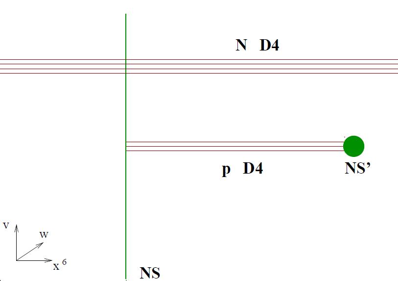
Figure 1: The brane system.

$$ds^{2} = H^{-1/3}\left(dx_{\mu}^{2}+dx_{6}^{2}+dx_{11}^{2}\right)+H^{2/3}\left(|dv|^{2}+|dw|^{2}+dx_{7}^{2}\right),$$

$$C_{6} = H^{-1}d^{4}x\wedge dx_{6}\wedge dx_{11},\qquad H=1+\frac{\pi\lambda_{N}l_{s}^{2}}{|\vec{r}-\vec{r}_{0}|^{3}}\,,$$ (146)

where $\lambda_{N}=g_{YM}^{2}N$ is the $4+1$ dimensional ‘t Hooft coupling. $\mu=0,1,2,3$, $\vec{r}=(v,w,x^{7})$ labels position in ${\rm I\kern-1.79993ptR}^{5}$, and $\vec{r}_{0}\in{\rm I\kern-1.79993ptR}^{5}$ is the position of the $N$ D4-branes in figure 1.

The shape of the curved fivebrane we are interested in is obtained by plugging in the ansatz

$$v=u(x_{6})e^{i\phi(x_{11})}\sin\alpha(x_{6}),\qquad w=u(x_{6})e^{-i\phi(x_{11})}\cos\alpha(x_{6}),$$ (147)

into the M5-brane worldvolume action. The induced metric on the fivebrane corresponding to (147) is

$$ds_{ind}^{2}=H^{-1/3}\left\{dx_{\mu}^{2}+\left[1+H\left((u\alpha^{\prime})^{2}+(u^{\prime})^{2}\right)\right]dx_{6}^{2}+\left(1+H(u{\dot{\phi}})^{2}\right)dx_{11}^{2}\right\},$$ (148)

where $u^{\prime}\equiv\partial_{x_{6}}u$, $\alpha^{\prime}\equiv\partial_{x_{6}}\alpha$ and $\dot{\phi}=\partial_{x_{11}}\phi$. The Lagrangian is

$$L=-H^{-1}\sqrt{1+H(u{\dot{\phi}})^{2}}\sqrt{1+H((u\alpha^{\prime})^{2}+(u^{\prime})^{2})}+H^{-1}.$$ (149)

The equations of motion imply that ${\dot{\phi}}$ must be constant; thus $\phi=x_{11}/pR=x_{11}/\lambda_{p}$. The Noether charges $J,P_{6}$ associated with the invariance under the shift of $\alpha$ and $x_{6}$, respectively, are then given by

$$J = \frac{u^{2}\alpha^{\prime}\sqrt{1+Hu^{2}/\lambda_{p}^{2}}}{\sqrt{1+H\left[(u\alpha^{\prime})^{2}+(u^{\prime})^{2}\right]}},$$

$$P_{6} = H^{-1}-\frac{H^{-1}\sqrt{1+Hu^{2}/\lambda_{p}^{2}}}{\sqrt{1+H\left[(u\alpha^{\prime})^{2}+(u^{\prime})^{2}\right]}}.$$ (150)

The profile of the probe M5 brane is described by the $v$ and $w$, which are expressed in terms of $u$ and $\alpha$ given in (147). The latter are determined by the effective 1+1 dimensional action $S=\int dtdx_{6}L$. The corresponding energy for a static configuration is $E=-S$.

Applying a uniform scaling deformation, and minimizing $E(\lambda)$, we get

$$\left.\frac{dE(\lambda)}{d\lambda}\right|_{\lambda=1}=\int dx\ H^{-1}\left\{1-\frac{\sqrt{1+Hu^{2}/\lambda_{p}^{2}}}{\sqrt{1+H\left[(u\alpha^{\prime})^{2}+(u^{\prime})^{2}\right]}}\right\}=0$$ (151)

The integrand is in fact the Noether charge density associated with the invariance under the shift $x_{6}\rightarrow x_{6}+a$ where $a$ is a constant. Stated differently, had we taken the action to be $0+1$ dimensional with $x_{6}$ as the time direction, the integrand would have been the energy density – as it is termed in [17]. The solution for the profile in [17] was taken to be the so-called supersymmetric profile where this “energy density” vanishes. The corresponding profile takes the form

$$u=\sqrt{\frac{J\lambda_{p}}{2}}\sqrt{2\cosh\frac{2x_{6}}{\lambda_{p}}},\qquad\tan\alpha=\exp\left(2x_{6}/\lambda_{p}\right),$$ (152)

which fulfills a Derrick-type condition. Requiring that the “energy density” associated with the shift invariance of a space coordinate should vanish, is equivalent to the Hamiltonian constraint. This occurs also in the applications to gravitational backgrounds discussed below. It is also easy to see that this holds in a more general setup. The reason Derrick’s condition coincides with the zero “energy” condition is that an infinitesimal dilatation is equivalent to an infinitesimal translation with a space-dependent parameter, so the term appearing in the variation of the energy is proportional to the generator of translations along $x$. Consider the following 1+1 dimensional Lagrangian density for $N$ degrees of freedom

$${\cal L}=-\sqrt{g_{0}(x)-\sum_{i=1}^{N}g_{i}[(\partial_{t}\phi_{i})^{2}-(\phi_{i}^{\prime})^{2}]}-V(\phi_{i})$$ (153)

For a static configuration, the energy density is ${\cal H}=-{\cal L}$ and Derrick’s condition reads

$$\left.\frac{dE(\lambda)}{d\lambda}\right|_{\lambda=1} = \int dx\ \left\{-\sqrt{g_{0}(\phi_{i})+\sum_{i=1}^{N}g_{i}[(\phi_{i}^{\prime})^{2}]}-V(\phi_{i})+\frac{\sum_{i=1}^{N}g_{i}[(\phi_{i}^{\prime})^{2}]}{\sqrt{g_{0}(x)+\sum_{i=1}^{N}g_{i}[(\phi_{i}^{\prime})^{2}]}}\right\}$$

$$= -\int dx\ \left\{V(\phi_{i})+\frac{g_{0}(\phi_{i})}{\sqrt{g_{0}(x)+\sum_{i=1}^{N}g_{i}[(\phi_{i}^{\prime})^{2}]}}\right\}=0\leavevmode\nobreak\ .$$

The expression in brackets is identical to the “energy” of the $0+1$ action where we have taken $x$ to be “time.”

5.2 Application to gravitational backgrounds

The DC on D-brane soliton solutions of super-gravity (SUGRA) actions are also interesting. The bosonic part of the SUGRA action in $D$ dimensions takes the form

$$S = \int d^{D}x\sqrt{G}e^{-2\phi}\left(R+4(\partial\phi)^{2}+\frac{c}{\alpha^{\prime}}\right)$$ (155)

$$-\frac{e^{-2\phi}}{2}\int H_{(3)}\wedge\star H_{(3)}-\sum_{p}\frac{1}{2}\int F_{(p+2)}\wedge\star F_{(p+2)},$$

where $\phi$ is the dilaton, $F_{p+2}$ is a RR form that corresponds to a Dp-brane with $n=p+1$ dimensional world volume, $H_{(3)}$ is the NS three form and $\frac{c}{\alpha^{\prime}}=\frac{10-D}{\alpha^{\prime}}$ is the non-criticality central charge term.

Let’s assume now that the metric in the string frame depends only on the radial coordinate $\tau$. It takes the form

$$l_{s}^{-2}ds^{2}=d\tau^{2}+e^{2\lambda(\tau)}dx_{\|}^{2}+e^{2\nu(\tau)}d\Omega_{k}^{2}$$ (156)

where $D=n+k+1$, $dx^{2}_{\|}$ is $n$ dimensional flat metric, and $d\Omega_{k}^{2}$ is a $k$ dimensional sphere.

Upon substituting the metric (156) into the action and performing the integration one finds[26]

$$S = l_{s}^{-2}\int d\rho\left(\left[-n(\lambda^{\prime})^{2}-k(\nu^{\prime})^{2}+(\varphi^{\prime})^{2}+ce^{-2\varphi}+(k-1)ke^{-2\nu-2\varphi}\right]\right)+S_{RR}+S_{NS}$$

$$S = l_{s}^{-2}\int d\rho\left(\left[-n(\lambda^{\prime})^{2}-k(\nu^{\prime})^{2}+(\varphi^{\prime})^{2}+ce^{-2\varphi}+(k-1)ke^{-2\nu-2\varphi}\right]\right.$$ (157)

$$\left.-Q_{RR}^{2}\rho e^{n\lambda-k\nu-\varphi}-Q_{NS}^{2}e^{-2k\nu-2\varphi}\right)$$

where $d\tau=-e^{-\varphi}d\rho$, $(A)^{\prime}=\partial_{\rho}A$ and $\varphi=2\phi-n\lambda-k\nu$ and the NS term is relevant only for $k=3$.

The action (5.2) can be viewed as a 1+1 dimensional action for three static scalar fields $\lambda,\nu$ and $\varphi$, subject to the potential

$$V=-(c+(k-1)ke^{-2\nu})e^{-2\varphi}+{Q_{RR}^{2}}e^{n\lambda-k\nu-\varphi}+Q_{NS}^{2}e^{-2k\nu-2\varphi}.$$ (158)

In fact the dimensionally reduced system is characterized not only by the action (5.2) but also by the so called “Hamiltonian constraint”, which is the Gauss’ law associated with fixing $g_{\tau\tau}=1$ and takes the following form

$${\cal H}=n(\partial_{\tau}\lambda)^{2}+k(\partial_{\tau}\nu)^{2}-(\partial_{\tau}\varphi)^{2}+c+(k-1)ke^{-2\nu}-Q_{RR}^{2}e^{n\lambda-k\nu+\varphi}-Q_{NS}^{2}e^{-2k\nu}=0.$$ (159)

Treating the system as that of 1+1 dimensional system of three scalar fields $\lambda,\nu,\varphi$ subjected to a potential , we are led to Derrick’s condition (33) that takes the form

$$\left.\frac{dE(\lambda)}{d\lambda}\right|_{\lambda=1} = \int d\tau\left[n(\partial_{\tau}\lambda)^{2}+k(\partial_{\tau}\nu)^{2}-(\partial_{\tau}\varphi)^{2}+c+(k-1)ke^{-2\nu}\right.$$ (160)

$$\left.-Q_{RR}^{2}e^{n\lambda-k\nu+\varphi}-Q_{NS}^{2}e^{-2k\nu}\right]$$

It is now straightforward to realize that the integrand of this integral is precisely the Hamiltonian constraint ${\cal H}=0$ and hence by construction static solutions of the system (5.2) is in accordance with Derrick’s theorem. These include the D-brane solitons of the critical theory as well as the D-brane solutions of non-critical dimensions[26].

5.3 Wilson lines

We noted above that finite-size spaces involve some subtleties in the DC language. We now describe how to study Wilson lines of finite length in this scheme, that we assume can be described using the Nambu-Goto action either in flat space or in a holographic setup. In principle the analysis can also be extended to probe branes with boundaries. In these cases, equation (9) may be modified by boundary terms.

Using the conservation of the energy-momentum tensor, $\partial_{i}\Pi^{i}_{\phantom{i}j}=0$ for some vector $\xi^{j}$,

$$\int_{\mathcal{M}}d^{d}x\ \partial_{i}(\xi^{j}\Pi^{i}_{\phantom{i}j})=\int_{\partial{\mathcal{M}}}d^{d-1}x\ \xi^{j}\hat{n}_{i}\Pi^{i}_{\phantom{j}j}\leavevmode\nobreak\ ,$$ (161)

where $\hat{n}$ is the normal to the spatial boundary of the manifold $\mathcal{M}$. Using $\xi^{j}=\lambda^{j}_{\phantom{j}k}x^{k}$ for arbitrary constant $\lambda^{j}_{\phantom{j}k}x^{k}$, this gives the conditions

$$\int_{\mathcal{M}}d^{d}x\ \Pi^{i}_{\phantom{i}j}=\int_{\partial{\mathcal{M}}}d^{d-1}x\ x^{i}\hat{n}_{k}\Pi^{k}_{\phantom{j}j}\leavevmode\nobreak\ .$$ (162)

The above expression holds for bounded spaces of arbitrary dimension. For the simple case of a Wilson line, there is only a single component in the stress tensor $\Pi^{1}_{\ 1}\equiv\Pi$. If the background metric does not depend explicitly on $x$, then the conservation (and lack of time dependence) for $\Pi$ implies that it is constant along the spatial direction $\partial_{x}\Pi=0$. We will assume that the coordinate $x$ is restricted to the interval $x\in[x_{1},x_{2}]$, and that there is a soliton solution with profile $Y^{a}(x)$, satisfying some fixed boundary conditions at the endpoints of the interval

$$F_{n}\left[Y^{a}(x_{n}),\partial_{x}Y^{a}(x_{n})\right]=0,\ \ n=1,2.$$ (163)

We now consider the deformed configuration $\tilde{Y}^{a}(x)=Y^{a}(\lambda x)$, in the interval with boundary at $\tilde{x}_{n}=x_{n}/\lambda$. Clearly, the new configuration will satisfy the following boundary conditions

$$F_{n}\left[\tilde{Y}^{a}(\tilde{x}_{n}),\frac{1}{\lambda}\partial_{x}\tilde{Y}^{a}(\tilde{x}_{n})\right]=0,\ \ n=1,2.$$ (164)

For both Dirichlet $F_{n}[Y,\partial Y]=Y-Y_{n}$ and Neumann $F_{n}[Y,\partial Y]=\partial Y$, the form of the boundary conditions is preserved. In the first case, the position of the endpoints in the ‘transverse’ directions remains fixed. Let us focus on this case in what follows.

It is convenient to write the energy of the soliton solution as an integral over the full real line

$$E[Y^{a}]=\int_{-\infty}^{\infty}d\sigma{\cal E}[Y^{a},\partial_{\sigma}Y^{a}]G[\sigma],$$ (165)

where ${\cal E}$ is the energy density and

$$G[\sigma]=\Theta(\sigma-x_{1})-\Theta(x_{2}-\sigma).$$ (166)

The deformed configuration preserving the Dirichlet boundary condition is $\tilde{Y}^{a}(\sigma)=Y^{a}(\lambda\sigma)$ and $\tilde{G}(\sigma)=G(\lambda\sigma)$. The energy is

$$E[\tilde{Y}^{a}]=\int_{-\infty}^{\infty}d\sigma{\cal E}[\tilde{Y}^{a},\partial_{\sigma}\tilde{Y}^{a}]\tilde{G}(\sigma).$$ (167)

We now rescale the spatial coordinate $\sigma\to\sigma/\lambda$, then

$$E[\tilde{Y}^{a}]=\int_{-\infty}^{\infty}d\sigma\frac{1}{\lambda}{\cal E}[Y^{a},\lambda\partial_{\sigma}Y^{a}]G(\sigma)=\int_{x_{1}}^{x_{2}}dx\frac{1}{\lambda}{\cal E}[Y^{a},\lambda\partial_{x}Y^{a}].$$ (168)

This leads to the usual result where the variation of the energy is proportional to the integral of the stress tensor

$$\delta E\sim\int_{x_{1}}^{x_{2}}dx\ \Pi=(x_{2}-x_{1})\Pi\equiv\Delta x\Pi\leavevmode\nobreak\ ,$$ (169)

where we have used the fact that $\Pi$ is constant. The variation is thus proportional to the length of the interval. This happens even for the ground state configuration because we are allowing the size of the interval to vary. For instance, if we think about the holographic calculation of a quark-antiquark potential, the deformed configuration still corresponds to a string ending at the AdS boundary, but the position of the endpoints along the spatial directions of the field theory is allowed to change. Clearly the energy is extremized when the two endpoints coincide and the string shrinks to zero size. This does not reflect a dynamical instability because the conserved quantity $\Pi$ is different for different sizes of the interval.

One should keep in mind that for the interesting case of Wilson lines in AdS backgrounds (as discussed at length in [27]), the bare energy derived from the action is not finite and must be renormalized. A Wilson line with its two endpoints on the AdS boundary will tend to dip down into the space. If one simply uses a subtraction scheme in which one subtracts off the energy, $E_{sub}$, of two straight Wilson lines to yield a finite energy, the analysis is completely unaffected.

An interesting extension of this analysis will be to introduce a deformed configuration with fixed boundary conditions in the same interval. However, this is not possible for a Dirichlet condition and the simple re-scaling presented here, where $\lambda$ is constant, since this would require that $\lambda(x_{n})=1$ at the endpoints of the interval.

6 Summary and open questions

The equations of motion of any interacting physical system are generically non-linear. There are only few cases for which exact solutions to these equations are known. It is thus interesting and important to derive constraints on physically realized solutions to these equations, as we have done here.

We have developed, analyzed and applied what we refer to as “deformation constraints” (DC). A special case of these constraints, used to prove Derrick’s theorem [9, 10], has been known for fifty years. Another class of constraints were proposed recently by Manton [11]. We rederived these two types of constraints by considering generalized deformations of energy-minimizing soliton solutions, including also internal symmetries. We have demonstrated the use of the DC in several soliton solutions like the magnetic monopole and the abelian Higgs model, and have obtained some novel results in the analysis of D-brane system solitons. We have applied the DC to a variety of D-brane actions that include the DBI as well as WZ terms. We have also discussed the application to flavor branes in M theory, Wilson lines and general static solutions of gravitational backgrounds. Other special cases that we have considered are non-linear generalizations of electromagnetism (of which the DBI action is a special case).

We have derived the following concrete constraints from the DC applied to branes:

• There can be no solitons of the DBI action (for arbitrary Dp-branes) in which the transverse directions depend only on one worldvolume coordinate.

• While solitons are excluded for Maxwell’s theory in four dimensions (4D), there is no such exclusion of solitons for DBI electromagnetism in 4D. Other non-linear generalizations may even admit magnetic solitons.

• For $D1$ branes with electric field in flat space-time, there are no BPS solutions living on the brane worldvolume.

• For $D2$ branes in flat space time, Abelian BPS vortices completely disappear if a magnetic field is turned on on the $D2$ brane.

The DC may serve as a useful tool for assessing classical static solutions in the context of “ordinary” field theories, D-brane models and gravity and string actions. The application of DC to other areas, and their extension to infinite-energy configurations, remain to be explored. We list some of these interesting directions here:

• We have considered solitons in field theory and D-brane models. There are a variety of other systems, however, in which these DC may find fruitful application.

  Solitonic configurations appear in optical[30] and magnetic systems, hydrodynamics and even in the physics of proteins and DNA. Soliton solutions exist also for equations of motion associated with non-relativistic actions which are not Lorentz invariant. As the DC represent a general framework for constraining finite energy static solutions, they make prove useful for identifying solutions of systems governed by the KDV and non-linear Schröedinger equations. One could also use the constraints to build new Lagrangians that admit (or exclude) solitons by design.

  It may also be interesting to continue the work of section §6, using the DC to search for gravitational solutions in cases where the kinetic terms and the “potential” are positive definite (which is not true of all gravitational systems). Other interesting extensions may include BIon-like solutions [18, 24] which are not fully smooth and have a singularity and an associated charge.

  The DC technique may even facilitate the solution of non-linear differential equations which are not necessarily related to physical systems. Given an equation, assume one can construct a Lagrangian density for which it is an equation of motion. One can then incorporate the time direction by adding a kinetic term to the Lagrangian density. The minimization of the corresponding energy with respect to deformations of the solutions will constitute a DC for this non-differential equation.

• Classical solutions of scalar field theories frequently appear in cosmology. In that case, one is not interested in static solutions but in solutions which are only time dependent. It may be possible to develop constraints similar to the DC for such configurations.

• Another related question is whether one can impose similar conditions by deforming solutions and minimizing energy for quantized solitons[31]. The main difference is that the classical energy can receive corrections from quantum fluctuations around the semiclassical soliton configuration. This configuration is in general different from the classical solution and requires solving the equation derived from the effective action in a self-consistent way.

• It was recently discovered[25, 28] that certain holographic models (both top-down and bottom-up) have ground states which are spatially modulated – that is, translational invariance is spontaneously broken. In these cases the energy is not finite. One must therefore develop new tools to apply the deformation constraints locally[29].

• Perhaps the best-known solitons are those associated with 1+1 dimensional models, such as the sine-Gordon model. This model is integrable. As a consequence, it – and others like it – admit an infinite set of conserved currents and associated charges. It would be interesting to generalize the DC to derive constraints on the spatial components of the infinite tower of conserved currents. It is not obvious a priori whether these higher order constraints will be independent, or whether they will follow automatically from the leading order constraints.

• The DC presented in section §2 include all possible spatial transformations that are linear in the coordinates. Special conformal transformations, which accompany scale transformations of any conformal invariant system, meanwhile, are quadratic in the coordinates at infinitesimal order. The quadratic deformations of the special conformal transformations can be generalized to any quadratic transformation, or as deformations at any order in the coordinates. These may imply the vanishing of integrals of the stress tensor multiplied by higher powers of the coordinates, implying a more rapid decay of the stress tensor at large radial coordinates.

• In section §2 we touched briefly on the relation between BPS configurations and the vanishing of the stress tensor. In these cases the stress tensor (not its integral) vanishes for all components. The interplay between the BPS condition, self-duality of solutions, and the vanishing of the stress tensor deserve further investigation, as do similar relations for global currents.

  For instance, BPS solitons are commonly defined as solutions that saturate the energy-charge bound. In supersymmetric theories this implies that they conserve half of the supersymmetries. One can then use the supersymmetric Ward identity to show that the components of the stress tensor vanish. However, one could define the soliton from the stress tensor, show that it must preserve half of the supersymmetries, and then recover the relation between the charge and the energy.

  In all of the examples we consider, BPS solitons break half of the supersymmetries. It would be interesting to consider whether the same conditions on the stress tensor are satisfied for solitons that break a larger number of supersymmetries.

Appendix A Examples of deformation constraints on branes

A.1 Probe branes in brane backgrounds

Particular examples where the brane action is finite for infinitely extended configurations happen when the DBI action is supplemented by a contribution from the RR fluxes that cancels out for trivial configurations. This is the case when we have a Dp-brane background, and compute the action for a Dp-probe in the background (extended along all of the same directions as the background branes). The near-horizon metric for the Dp background takes the form

$$ds^{2}=\left(\frac{R}{r}\right)^{(7-p)/2}dr^{2}+\left(\frac{r}{R}\right)^{(7-p)/2}\eta_{\mu\nu}dx^{\mu}dx^{\nu}+R^{2}\left(\frac{r}{R}\right)^{(p-3)/2}d\Omega_{8-p}^{2}.$$ (170)

Here $d\Omega_{8-p}^{2}$ is the metric of a unit $(8-p)$-sphere, $S^{8-p}$. The “conformal boundary” is at $r\to\infty$. The dilaton has the form

$$e^{\phi}=e^{\phi_{0}}\left(\frac{R}{r}\right)^{(7-p)(3-p)/4}.$$ (171)

The potential for $F_{p+2}=dC_{p+1}$ takes the form

$$C_{p+1}=\frac{1}{g_{s}}\left(\frac{r}{R}\right)^{7-p}dx^{0}\wedge\cdots\wedge dx^{p}.$$ (172)

The action on the probe $Dp$-branes, adding both DBI and WZ terms is

$$S =-T_{p}\int d^{p+1}x\left[e^{-\phi}\sqrt{-g}-C_{p+1}\right]=-\frac{T_{p}}{g_{s}}\int d^{p+1}x\left[\sqrt{-g}-\left(\frac{r}{R}\right)^{7-p}\right].$$ (173)

We will restrict now to the simplest case where we assume that the soliton is determined by a function $r(x^{1})$ describing the change in the radial position of the brane along a single spatial direction. The embedding is

$$X^{\mu}=x^{\mu},\ \ Y^{p+1}=r(x^{1}),\ \ Y^{a>p+1}=0.$$ (174)

The action becomes (with $R=1$ for simplicity)

$$S=-\int d^{p+1}xL=-\int d^{p+1}xr^{7-p}\left[\sqrt{1+r^{p-7}{r^{\prime}}^{2}}-1\right].$$ (175)

The energy density is simply minus the Lagrangian density

$$E=\int d^{p}xr^{7-p}\left[\sqrt{1+r^{p-7}{r^{\prime}}^{2}}-1\right].$$ (176)

We now follow Derrick’s procedure and evaluate the energy for the rescaled configuration $r(\lambda x^{1})$, where we assume that $r(x)$ is a solution to the equations of motion. After we change coordinates $x^{1}\to x^{1}/\lambda$ the energy becomes

$$E(\lambda)=\int d^{p}x\lambda^{-p}r^{7-p}\left[\sqrt{1+\lambda^{2}r^{p-7}{r^{\prime}}^{2}}-1\right].$$ (177)

Then, Derrick’s condition is

$$0=\left.\frac{dE}{d\lambda}\right|_{\lambda=1}=\int d^{p}x\left(-pL+\frac{{r^{\prime}}^{2}}{\sqrt{1+r^{p-7}{r^{\prime}}^{2}}}\right).$$ (178)

Note that for $r^{\prime}=0$ we have that $L=0$, so this is satisfied for the trivial solution, but as we saw in the general analysis soliton solutions are not discarded in principle. However, we will show that they are actually not allowed by showing that if Derrick’s condition was satisfied, the solution would not be a minimum of the energy, but rather a maximum. First note that if there is a solitonic solution it must be true that

$$L=\frac{1}{p}\frac{{r^{\prime}}^{2}}{\sqrt{1+r^{p-7}{r^{\prime}}^{2}}}.$$ (179)

We now take the second derivative of the energy

$$\left.\frac{d^{2}E}{d\lambda^{2}}\right|_{\lambda=1}=\int d^{p}x\left(p(p+1)L-(2p-1)\frac{{r^{\prime}}^{2}}{\sqrt{1+r^{p-7}{r^{\prime}}^{2}}}-\frac{{r^{\prime}}^{4}}{(1+r^{p-7}{r^{\prime}}^{2})^{3/2}}\right).$$ (180)

Solving for $L$ using (179) we have that

$$\left.\frac{d^{2}E}{d\lambda^{2}}\right|_{\lambda=1}=\int d^{p}x\left(-(p-2)\frac{{r^{\prime}}^{2}}{\sqrt{1+r^{p-7}{r^{\prime}}^{2}}}-\frac{r^{p-7}{r^{\prime}}^{4}}{(1+r^{p-7}{r^{\prime}}^{2})^{3/2}}\right).$$ (181)

This is negative for $p\geq 2$, which means there are no solitonic configurations of this kind. For $p=1$

$$\left.\frac{d^{2}E}{d\lambda^{2}}\right|_{\lambda=1}=\int dx\frac{{r^{\prime}}^{2}}{\sqrt{1+r^{-6}{r^{\prime}}^{2}}}\left(1-\frac{r^{-6}{r^{\prime}}^{2}}{1+r^{-6}{r^{\prime}}^{2}}\right)=\int dx\frac{{r^{\prime}}^{2}}{(1+r^{-6}{r^{\prime}}^{2})^{3/2}}.$$ (182)

which is manifestly positive, so solitons are in principle allowed for D1 branes even taking into account this more restrictive condition. A question is whether the extremality condition can actually be satisfied once we use the equations of motion. The answer is yes, but for the D1 brane

$$\left.\frac{dE}{d\lambda}\right|_{\lambda=1}\sim-L+\frac{{r^{\prime}}^{2}}{\sqrt{1+r^{-6}{r^{\prime}}^{2}}}=\frac{\delta L}{\delta r^{\prime}}r^{\prime}-L\equiv\pi^{x},$$ (183)

which is just a constant of motion for the D1 brane. The extremality condition requires $\pi^{x}=0$. However this gives as a solution $r^{\prime}=0$, so there are actually no solitons.

Although we have ruled out only a very restricted class of configurations, this shows explicitly that Derrick’s condition can be naturally extended to impose much stronger constraints.

A.2 D3 brane with electric and magnetic fields

Before imposing Derrick’s conditions on the DBI action recall the conditions on the ordinary Maxwell theory. The energy is

$$E=\frac{1}{2}\int d^{d}x[(\vec{B})^{2}+(\vec{E})^{2}].$$ (184)

The scaling of the electric and magnetic field as above, namely, $\vec{E}\rightarrow\lambda\vec{E}$ and $\vec{B}\rightarrow\lambda^{2}\vec{B}$. Thus the scaled energy is

$$E(\lambda)=\frac{1}{2}\int d^{d}x\lambda^{-d}[\lambda^{4}(\vec{B})^{2}+\lambda^{2}(\vec{E})^{2}].$$ (185)

Derrick’s condition is therefore

$$\left.\frac{dE(\lambda)}{d\lambda}\right|_{\lambda=1}=\frac{1}{2}\int d^{d}x[(4-d)(\vec{B})^{2}-(d-2)(\vec{E})^{2}]=0.$$ (186)

For $d=3$ spatial dimensions (anti) self-dual configurations with $\vec{E}=\pm\vec{B}$ obviously fulfill Derrick’s condition but as usual the actual condition is that the integral and not necessarily the integrand will vanish.

We assume as background fields $C_{012}=e^{-\phi}=1$ in order to have finite energy configurations. For simplicity we will assume that the scalar fields are trivial. The corresponding action in flat space takes the form

$$S_{DBI}=T_{3}\int d^{4}x\left[1-\sqrt{1-(\vec{E})^{2}+(\vec{B})^{2}-(\vec{E}\cdot\vec{B})^{2}}\right].$$ (187)

The energy density associated with this action reads

$${\cal E}=\sqrt{1+(\vec{B})^{2}+(\vec{D})^{2}+(\vec{B}\times\vec{D})^{2}}-1,$$ (188)

where $\vec{D}$ is given by $\frac{\partial{\cal L}}{\partial\vec{E}}$. Consider first the case of only magnetic fields turned on. In this case

$${\cal L}=1-\sqrt{1+(\vec{B})^{2}}\qquad{\cal E}=\sqrt{1+(\vec{B})^{2}}-1$$ (189)

The scaled energy is

$$E_{B}=\int d^{3}x\lambda^{-3}(\sqrt{1+\lambda^{4}(\vec{B})^{2}}-1)$$ (190)

The condition for a finite energy static magnetic field thus takes the form

$$\left.\frac{dE_{B}(\lambda)}{d\lambda}\right|_{\lambda=1}=\int d^{3}x\left[3-\frac{3+(\vec{B})^{2}}{\sqrt{1+(\vec{B})^{2}}}\right]=0$$ (191)

Note that whereas for a magnetic field in Maxwell theory we have $E(\lambda)=\int d^{3}x\lambda(\vec{B})^{2}$ and hence Derrick’s condition cannot be fulfilled, for the magnetic field in DBI there is no such an obvious objection. It is easy to check that by expanding the square root to leading order one recovers the result in Maxwell’s theory.

Next we consider the case of an electric field. For such a case we have a scaled energy

$$E_{E}=\int d^{3}x\lambda^{-3}\left[\frac{1}{\sqrt{1-\lambda^{2}(\vec{E})^{2}}}-1\right].$$ (192)

Derrick’s condition now reads

$$\left.\frac{dE_{E}(\lambda)}{d\lambda}\right|_{\lambda=1}=\int d^{3}x\left[3+\frac{-3+2(\vec{E})^{2}}{\sqrt{(1-(\vec{E})^{2})^{3}}}\right]=0.$$ (193)

Again, this condition does not exclude a static finite energy solution as it does for Maxwell theory. Furthermore, one can easily show that the second derivative (for the allowed values of $0\leq E^{2}\leq 1$) is always negative, so any solution satisfying the above will lie at a minimum of the energy.

For the general case of both electric and magnetic field the scaled energy reads

$$E=\int d^{3}x\lambda^{-3}\left[\sqrt{1+\lambda^{4}[\vec{B})^{2}+(\vec{D}(\lambda))^{2}+\lambda^{4}(\vec{B}\times\vec{D}(\lambda))^{2}]}-1\right],$$ (194)

where

$$\vec{D}(\lambda)=\frac{\lambda(\vec{E}+\lambda^{4}(\vec{E}\cdot\vec{B})\vec{B})}{\sqrt{1+\lambda^{2}[\lambda^{2}(\vec{B})^{2}-(\vec{E})^{2}-\lambda^{4}(\vec{B}\cdot\vec{E})^{2}]}}.$$ (195)

Upon substituting $D(\lambda)$ into (194) we find that

$$E=\int d^{3}x\lambda^{-3}\left[\frac{1+\lambda^{4}B^{2}}{\sqrt{1-\lambda^{2}[(\vec{E})-\lambda^{2}(\vec{B})^{2}+\lambda^{4}(\vec{E}\cdot\vec{B})^{2}]}}-1\right],$$ (196)

which reduces to (189) and (192) when the electric and magnetic fields are switched off, respectively. Derrick’s condition thus takes the form

$$\left.\frac{dE(\lambda)}{d\lambda}\right|_{\lambda=1}=\int d^{3}x\left[3-\frac{3+4(\vec{B})^{2}-6(\vec{E}\cdot\vec{B})^{2}-4(\vec{E})^{2}+(\vec{B})^{2}((\vec{B})^{2}-2(\vec{E}\cdot\vec{B})^{2})}{\sqrt{(1-(\vec{E})^{2}+(\vec{B})^{2}-(\vec{E}\cdot\vec{B})^{2})^{3}}}\right].$$ (197)

Though solitons are not excluded, it is interesting to note that one naive ansatz, in which $\vec{E}$ and $\vec{B}$ are orthogonal but have the same magnitude is excluded by this constraint. If we take $|\vec{E}|=|\vec{B}|$ but $\vec{E}\cdot\vec{B}=0$, we find

$$\left.\frac{dE(\lambda)}{d\lambda}\right|_{\lambda=1}=-\int d^{3}xB^{4}<0\leavevmode\nobreak\ ,$$ (198)

so no non-trivial solutions can minimize the energy.

Appendix B Deformation constraints in DBI with scalars

We show more explicitly here that the Derrick or Manton constraints do not exclude the possibility of scalar solitons in the DBI action. Recall equation 76. To simplify it a bit further, it will be useful to write the pullback metric as

$$g_{ij}=G_{ik}N^{k}_{\ j}=G_{ik}\left[\delta^{k}_{\ j}+\hat{G}^{kl}G_{ab}\partial_{l}Y^{a}\partial_{j}Y^{b}\right]=(\hat{G}N)_{ij}.$$ (199)

The hat denotes inversion with respect to only the spatial part of the metric: $\hat{G}^{ik}G_{kj}=\delta^{i}_{\ j}$. Let us also define $\hat{g}^{ik}g_{kj}=\delta^{i}_{\ j}$. The matrix $N$ is the sum of two positive definite matrices,

$$N=I+\hat{G}^{-1}(Y\cdot Y),$$ (200)

so it is possible diagonalize it at any point in space. The eigenvalues are of the form $1+\lambda_{i}$, with $\lambda_{i}\geq 0$. This implies that $\sqrt{-\det g}>\sqrt{-\det G}$, and the sum of the first two terms in the parentheses in (76) is positive. In order to cancel this, the space average of the inverse metric must satisfy

$$T_{p}\sum_{l}\int d^{p}xe^{\epsilon\phi}\sqrt{-\det{g}}g^{il}(g_{il}-G_{il})>0$$ (201)

where we use the inverse of the pullback metric,

$$g^{\mu\nu}=\frac{1}{G_{00}-\hat{g}^{kl}G_{0k}G_{0l}}\left(\begin{array}[]{cc}1&-\hat{g}^{jn}G_{0n}\\ -\hat{g}^{im}G_{0m}&(G_{00}-\hat{g}^{kl}G_{0k}G_{0l})\hat{g}^{ij}+\hat{g}^{ik}\hat{g}^{jl}G_{0k}G_{0l}\end{array}\right).$$ (202)

If we consider the case where we scale all the spatial coordinates with the same factor $\lambda_{i}=\lambda$ (Derrick’s condition), we can see that this is, in principle, possible. We now have

$$g^{ij}(g_{ij}-G_{ij})>0,$$ (203)

where now summation is implied. Then,

$$g^{ij}(g_{ij}-G_{ij})={\rm tr}\,(\hat{g}^{-1}(\hat{g}-\hat{G}))+\delta=p-{\rm tr}\,((N^{-1}\hat{G}^{-1})\hat{G})+\delta=p-{\rm tr}\,(N^{-1})+\delta.$$ (204)

Where we have defined

$$\delta=\frac{\hat{g}^{kl}G_{0k}G_{0l}-G_{ij}\hat{g}^{ik}\hat{g}^{jl}G_{0k}G_{0l}}{G_{00}-\hat{g}^{kl}G_{0k}G_{0l}}.$$ (205)

so the weakest condition we know must be satisfied is

$$p-{\rm tr}\,(N^{-1})+\delta>0.$$ (206)

Since the eigenvalues of $M$ are larger than one, the eigenvalues of $M^{-1}$ are smaller than one, so the condition (206) could be satisfied by a nontrivial configuration, even in the absence of additional fluxes. This does not, therefore, explicitly exclude the possibility of having non-trivial scalar solitons. We reach a similar conclusion if we try to impose Derrick’s condition for $G_{0i}=0$,

$$\sqrt{-\det g}-\sqrt{-\det G}=g^{ij}(g_{ij}-G_{ij}).$$ (207)

This condition can be written in terms of the matrix $N$ as

$$\operatorname{tr\>}(N^{-1})=\frac{p}{\sqrt{\det N}}.$$ (208)

For $p=1$ the only solution is $N=I$. For $p=2$ we already find more possibilities. In terms of the eigenvalues of $N$ we get the condition

$$\frac{1}{1+\lambda_{1}}+\frac{1}{1+\lambda_{2}}=\frac{2}{\sqrt{(1+\lambda_{1})(1+\lambda_{2})}}.$$ (209)

This is automatically satisfied if $\lambda_{1}=\lambda_{2}$. In general for $p>1$ the conditions can be written as a polynomial equation for the eigenvalues, after squaring the original condition

$$\left(\sum_{i=1}^{p}\frac{1}{1+\lambda_{i}}\right)^{2}=\frac{p^{2}}{\prod_{i=1}^{p}(1+\lambda_{i})}.$$ (210)

References

- [1] For a review see for instance: S. Coleman “Aspects of Symmetry” selected Erice lectures of Sindney Coleman Cambridge University Cambridge, U.K R. Rajaraman, “ An Introduction to Solitons and Instantons in Quantum FIeld Theory” (1982) North Holland, Amsterdam.
- [2] H. B. Nielsen and P. Olesen, “Vortex Line Models for Dual Strings,” Nucl. Phys. B 61, 45 (1973).
- [3] H. J. de Vega and F. A. Schaposnik, “A Classical Vortex Solution of the Abelian Higgs Model,” Phys. Rev. D 14 (1976) 1100.
- [4] G. ’t Hooft, “Magnetic Monopoles in Unified Gauge Theories,” Nucl. Phys. B 79 (1974) 276.
- [5] A. M. Polyakov, “Particle Spectrum in the Quantum Field Theory,” JETP Lett. 20 (1974) 194 [Pisma Zh. Eksp. Teor. Fiz. 20 (1974) 430].
- [6] T. H. R. Skyrme, “A Unified Field Theory of Mesons and Baryons,” Nucl. Phys. 31, 556 (1962).
- [7] G. S. Adkins, C. R. Nappi and E. Witten, “Static Properties of Nucleons in the Skyrme Model,” Nucl. Phys. B 228 (1983) 552.
- [8] H. Hata, T. Sakai, S. Sugimoto and S. Yamato, “Baryons from instantons in holographic QCD,” Prog. Theor. Phys. 117, 1157 (2007) [hep-th/0701280 [HEP-TH]].
- [9] G. H. Derrick, “Comments on nonlinear wave equations as models for elementary particles,” J. Math. Phys. 5 (1964) 1252.
- [10] R. H. Hobart, “On the Instability of a Class of Unitary Field Models,” Proc. Phys. Soc. 82 (1963) 201.
- [11] N. S. Manton, “Scaling Identities for Solitons beyond Derrick’s Theorem,” J. Math. Phys. 50 (2009) 032901 [arXiv:0809.2891 [hep-th]].
- [12] R. Jackiw, “Semiclassical Analysis of Quantum Field Theory,” PRINT-76-0982 (MIT).
- [13] L. D. Faddeev, L. Freyhult, A. J. Niemi and P. Rajan, “Shafranov’s virial theorem and magnetic plasma confinement,” J. Phys. A 35 (2002) L133 [physics/0009061].
- [14] D. Harland, M. Speight and P. Sutcliffe, “Hopf solitons and elastic rods,” Phys. Rev. D 83, 065008 (2011) [arXiv:1010.3189 [hep-th]].
- [15] S. Endlich, K. Hinterbichler, L. Hui, A. Nicolis, J. Wang and , “Derrick’s theorem beyond a potential,” JHEP 1105, 073 (2011) [arXiv:1002.4873 [hep-th]].
- [16] A. Padilla, P. M. Saffin, S. -Y. Zhou and , “Multi-galileons, solitons and Derrick’s theorem,” Phys. Rev. D 83, 045009 (2011) [arXiv:1008.0745 [hep-th]].
- [17] O. Aharony, D. Kutasov, O. Lunin, J. Sonnenschein and S. Yankielowicz, “Holographic MQCD,” Phys. Rev. D 82 (2010) 106006 [arXiv:1006.5806 [hep-th]].
- [18] G. W. Gibbons, “Born-Infeld particles and Dirichlet p-branes,” Nucl. Phys. B 514, 603 (1998) [hep-th/9709027].
- [19] E. B. Bogomolny, “Stability of Classical Solutions,” Sov. J. Nucl. Phys. 24, 449 (1976) [Yad. Fiz. 24, 861 (1976)].
- [20] M. K. Prasad and C. M. Sommerfield, “An Exact Classical Solution for the ’t Hooft Monopole and the Julia-Zee Dyon,” Phys. Rev. Lett. 35, 760 (1975).
- [21] E. F. Moreno and F. A. Schaposnik, “BPS Equations and the Stress Tensor,” Phys. Lett. B 673, 72 (2009) [arXiv:0811.2359 [hep-th]].
- [22] For a review of the topological currents see for instance Y. Frishman and J. Sonnenschein, “Non-perturbative field theory: From two-dimensional conformal field theory to QCD in four dimensions,” Cambridge, UK: Univ. Pr. (2010) 436 p
- [23] G. Date, Y. Frishman and J. Sonnenschein, “The Spectrum Of Multiflavor Qcd In Two-dimensions,” Nucl. Phys. B 283 (1987) 365.
- [24] C. G. Callan and J. M. Maldacena, “Brane death and dynamics from the Born-Infeld action,” Nucl. Phys. B 513, 198 (1998) [hep-th/9708147].
- [25] J. P. Gauntlett, J. Gomis and P. K. Townsend, “BPS bounds for world volume branes,” JHEP 9801, 003 (1998) [hep-th/9711205].
- [26] S. Kuperstein and J. Sonnenschein, “Noncritical supergravity () and holography,” JHEP 0407 (2004) 049 [hep-th/0403254].
- [27] U. Kol and J. Sonnenschein, “Can holography reproduce the QCD Wilson line?,” JHEP 1105, 111 (2011) [arXiv:1012.5974 [hep-th]].
- [28] S. Nakamura, H. Ooguri and C. -S. Park, “Gravity Dual of Spatially Modulated Phase,” Phys. Rev. D 81, 044018 (2010) [arXiv:0911.0679 [hep-th]].
- [29] S. K. Domokos, C. Hoyos and J. Sonnenschein in preparation.
- [30] For a review see for instance Y. Kivshara and B. Luther-Daviesb “Dark optical solitons: physics and applications” Physics Reports Volume 298, Issues 2 1 7 1 May 1998, Pages 81 1 77
- [31] R. F. Dashen, B. Hasslacher and A. Neveu, “Nonperturbative Methods and Extended Hadron Models in Field Theory. 2. Two-Dimensional Models and Extended Hadrons,” Phys. Rev. D 10 (1974) 4130.