Abstract

The process of exciting the gas of trapped bosons from an equilibrium initial state to strongly nonequilibrium states is described as a procedure of symmetry restoration caused by external perturbations. Initially, the trapped gas is cooled down to such low temperatures, when practically all atoms are in Bose-Einstein condensed state, which implies the broken global gauge symmetry. Excitations are realized either by imposing external alternating fields, modulating the trapping potential and shaking the cloud of trapped atoms, or it can be done by varying atomic interactions by means of Feshbach resonance techniques. Gradually increasing the amount of energy pumped into the system, which is realized either by strengthening the modulation amplitude or by increasing the excitation time, produces a series of nonequilibrium states, with the growing fraction of atoms for which the gauge symmetry is restored. In this way, the initial equilibrium system, with the broken gauge symmetry and all atoms condensed, can be excited to the state, where all atoms are in the normal state, with completely restored gauge symmetry. In this process, the system, starting from the regular superfluid state, passes through the states of vortex superfluid, turbulent superfluid, heterophase granular fluid, to the state of normal chaotic fluid in turbulent regime. Both theoretical and experimental studies are presented.

1 Introduction

Different thermodynamic phases are usually characterized by different symmetries. At the point of a phase transition, there occurs the change of system symmetry [1, 2, 3]. The observation of phase transitions can be done by slowly varying the system parameters, e.g., temperature, pressure, density, or some stationary external fields, so that the system practically always is in equilibrium

Another possibility of observing phase transitions is to prepare a system in a nonequilibrium phase under the values of parameters favoring a different phase. Then the system, starting from one phase with a given symmetry, relaxes to the equilibrium phase with another symmetry, dynamically passing through the phase-transition line [4].

In the present paper, we suggest and study the third way of realizing phase transitions accompanied by symmetry changes. This way is opposite to the relaxation procedure. We can start from an equilibrium phase, with one type of symmetry, and then pump into the system energy by means of external alternating fields, so that to transfer the system into another state, with another symmetry type. We illustrate this idea by considering the system of trapped bosons. This system can be cooled down to very low temperatures below the Bose-Einstein condensation point, when all atoms pile down to the condensed state. The properties of these condensed atoms have been intensively studied both theoretically and experimentally, as can be inferred from the books [5, 6, 7, 8] and reviews [9, 10, 11, 12, 13, 14, 15, 16, 17, 18, 19, 20].

The Bose-condensed state is characterized by the global gauge symmetry breaking. Moreover, the latter is the necessary and sufficient condition for Bose-Einstein condensation [6, 15]. Acting on the system of trapped atoms by external alternating fields increases the system energy, which is similar to increasing the system temperature. The energy, pumped into the system, destroys the condensate, transferring atoms into uncondensed states. When the injected energy is very large, one should expect that the state can be reached where all condensate has been depleted, and the whole system is in the normal phase, with the restored gauge symmetry. This latter state will, of course, be nonequilibrium, being reached by subjecting the system with time-dependent alternating fields. The investigation of such a procedure of nonequilibrium transitions, going through several stages, is the aim of the present paper. We shall describe both theoretical as well as experimental peculiarities of this method. The main part of the paper summarizes the results of previous publications, while some experimental results, related to the granular state, are new.

2 Broken Gauge Symmetry

We consider a system of spinless bosons characterized by the field operators $\hat{\psi}({\bf r},t)$ satisfying Bose commutation relations. Here ${\bf r}$ is spatial variable and $t$ is time. In the equations below, for the compactness of notation, we often omit the time variable, assuming it but writing the field operator as $\hat{\psi}({\bf r})$, when this does not lead to confusion. We keep in mind dilute Bose gas confined in a trap modelled by an external trapping potential $U=U({\bf r},t)$. Atomic interactions are described by the local potential

$$\Phi({\bf r})=\Phi_{0}\delta({\bf r})\;,\qquad\Phi_{0}\equiv 4\pi\;\frac{a_{s}}{m}\;,$$ (1)

where $a_{s}$ is scattering length and $m$, atomic mass. The scattering length, for concreteness, is assumed to be positive. Generally, it could be negative, but then the number of atoms should be such that to avoid the collapse occurring for atoms with attractive interactions.

Here and in what follows, we shall use in the majority of equations, the system of units with the Planck and Boltzmann constants set to one $(\hbar=1,k_{B}=1)$.

The external potential consists of two terms,

$$U({\bf r},t)=U({\bf r})+V({\bf r},t)\;,$$ (2)

the first term being the trapping potential and the second term describing additional modulation potential pumping energy into the trap.

The energy operator is given by the standard Hamiltonian

$$\hat{H}=\int\hat{\psi}({\bf r})\left(-\;\frac{\nabla^{2}}{2m}+U\right)\hat{\psi}({\bf r})\;d{\bf r}+\frac{\Phi_{0}}{2}\int\hat{\psi}^{\dagger}({\bf r})\hat{\psi}^{\dagger}({\bf r})\hat{\psi}({\bf r})\hat{\psi}({\bf r})\;d{\bf r}\;,$$ (3)

where $U$ is the total external potential (2). In the presence of Bose-Einstein condensate, the system global gauge symmetry is necessarily broken [6, 15]. The most convenient way of breaking the gauge symmetry is by employing the Bogolubov shift [21, 22] of the field operator:

$$\hat{\psi}({\bf r})=\eta({\bf r})+\psi_{1}({\bf r})\;,$$ (4)

in which $\eta({\bf r})$ is the condensate wave function normalized to the number of condensed atoms

$$N_{0}=\int|\eta({\bf r})|^{2}d{\bf r}\;,$$ (5)

and $\psi_{1}({\bf r})$ is the operator of uncondensed atoms defining their number

$$N_{1}=\langle\hat{N}_{1}\rangle\;,\qquad\hat{N}_{1}\equiv\int\psi_{1}^{\dagger}({\bf r})\psi_{1}({\bf r})\;d{\bf r}\;,$$ (6)

with the angle brackets implying statistical averaging. By this definition, the field operator of uncondensed atoms satisfies the Bose commutation relations.

The condensate function and the field operator of uncondensed atoms characterize different degrees of freedom, orthogonal to each other,

$$\int\eta^{*}({\bf r})\psi_{1}({\bf r})\;d{\bf r}=0\;.$$

The condensate function plays the role of the system order parameter, such that

$$\langle\hat{\psi}({\bf r})\rangle=\eta({\bf r})\;,\qquad\langle\psi_{1}({\bf r})\rangle=0\;.$$ (7)

This definition can also be written in the form of the statistical average

$$\langle\hat{\Lambda}\rangle=0$$ (8)

of the operator

$$\hat{\Lambda}\equiv\int\left[\lambda({\bf r})\psi_{1}^{\dagger}({\bf r})+\lambda^{*}({\bf r})\psi_{1}({\bf r})\right]\;d{\bf r}\;,$$ (9)

in which $\lambda({\bf r})$ is a Lagrange multiplier guaranteeing the validity of condition (7).

The correct description of any statistical system presupposes the use of the representative ensemble uniquely defining the system [20, 23, 24, 25]. This requires to take into account all imposed constraints that, in the present case, are given by Eqs. (5), (6), and (8). In turn, taking account of these constraints makes it necessary to introduce the grand Hamiltonian

$$H=\hat{H}-\mu_{0}N_{0}-\mu_{1}\hat{N}_{1}-\hat{\Lambda}\;,$$ (10)

with the Lagrange multipliers $\mu_{0}$ and $\mu_{1}$. Only employing this grand Hamiltonian allows one to correctly describe the Bose-condensed system. When one uses an ensemble that is not representative, that is, when not all constraints are taken into account, this leads to various inconsistencies in thermodynamic and dynamic characteristics, such as the arising gap in the spectrum of elementary excitations and instability of the system.

3 Nonequilibrium Bose System

In the presence of an external time-dependent potential, we have to study a nonequilibrium Bose system. The equations of motion for the system variables can be written through the variational derivatives, which is equivalent to the Heisenberg equations of motion [20, 26]. The condensate function satisfies the equation

$$i\;\frac{\partial}{\partial t}\;\eta({\bf r},t)=\left\langle\frac{\delta H}{\delta\eta^{*}({\bf r},t)}\right\rangle\;.$$ (11)

While for the field operator of uncondensed atoms, one has

$$i\;\frac{\partial}{\partial t}\;\psi_{1}({\bf r},t)=\frac{\delta H}{\delta\psi_{1}^{\dagger}({\bf r},t)}\;.$$ (12)

To represent the resulting evolution equations in a convenient form, let us introduce several notations. The condensate density is

$$\rho_{0}({\bf r})\equiv|\eta({\bf r})|^{2}\;.$$ (13)

The density of uncondensed atoms reads as

$$\rho_{1}({\bf r})\equiv\langle\psi_{1}^{\dagger}({\bf r})\psi_{1}({\bf r})\rangle\;.$$ (14)

When the gauge symmetry is broken, there appear the anomalous averages, such as the pair anomalous average

$$\sigma_{1}({\bf r})\equiv\langle\psi_{1}({\bf r})\psi_{1}({\bf r})\rangle$$ (15)

and the triple anomalous averages

$$\xi({\bf r})\equiv\langle\psi_{1}^{\dagger}({\bf r})\psi_{1}({\bf r})\psi_{1}({\bf r})\rangle\;,\qquad\xi_{1}({\bf r})\equiv\langle\psi_{1}({\bf r})\psi_{1}({\bf r})\psi_{1}({\bf r})\rangle\;.$$ (16)

The total atomic density is the sum

$$\rho({\bf r})=\rho_{0}({\bf r})+\rho_{1}({\bf r})\;.$$ (17)

Equation (11) yields the equation for the condensate function

$$i\;\frac{\partial}{\partial t}\;\eta({\bf r})=\left(-\;\frac{\nabla^{2}}{2m}+U-\mu_{0}\right)\eta({\bf r})+\Phi_{0}\left[\rho_{0}({\bf r})\eta({\bf r})+2\rho_{1}({\bf r})\eta({\bf r})+\sigma_{1}({\bf r})\eta^{*}({\bf r})+\xi({\bf r})\right]\;.$$ (18)

And using Eq. (12), we find the continuity equation for the density of uncondensed atoms,

$$\frac{\partial}{\partial t}\;\rho_{1}({\bf r})+{\bf\nabla}\cdot{\bf j}_{1}({\bf r})=-\Gamma({\bf r})\;,$$ (19)

with the atomic current

$${\bf j}_{1}({\bf r})\equiv-\;\frac{i}{2m}\left\langle\psi_{1}^{\dagger}({\bf r}){\bf\nabla}\psi_{1}({\bf r})-\left[{\bf\nabla}\psi_{1}^{\dagger}({\bf r})\right]\psi_{1}({\bf r})\right\rangle$$ (20)

and the source term given by the expression

$$\Gamma({\bf r})=i\Phi_{0}\left[\Xi^{*}({\bf r})-\Xi({\bf r})\right]\;,$$ (21)

in which

$$\Xi({\bf r})\equiv\eta^{*}({\bf r})\left[\eta^{*}({\bf r})\sigma_{1}({\bf r})+\xi({\bf r})\right]\;.$$ (22)

In addition, it is necessary to consider the equations for the anomalous averages. Writing down the equation for the pair average (15), we can use the Hartree-Fock-Bogolubov approximation for the four-operator correlator

$$\langle\psi_{1}^{\dagger}({\bf r})\psi_{1}({\bf r})\psi_{1}({\bf r})\psi_{1}({\bf r})\rangle=3\rho_{1}({\bf r})\sigma_{1}({\bf r})\;.$$ (23)

Also, we define the anomalous kinetic term

$$K({\bf r})\equiv-\;\frac{1}{2}\left\langle\frac{\nabla^{2}\psi_{1}({\bf r})}{2m}\;\psi_{1}({\bf r})+\psi_{1}({\bf r})\;\frac{\nabla^{2}\psi_{1}({\bf r})}{2m}\right\rangle\;=$$

$$=\;\frac{1}{2m}\left\{\left\langle[\nabla\psi_{1}({\bf r})^{2}]\right\rangle-\;\frac{1}{2}\;\nabla^{2}\sigma_{1}({\bf r})\right\}\;.$$ (24)

Then the evolution equation for the anomalous average (15) is

$$i\;\frac{\partial}{\partial t}\;\sigma_{1}({\bf r})=2K({\bf r})+2(U-\mu_{1})\sigma_{1}({\bf r})\;+$$

$$+\;2\Phi_{0}\left[\eta^{2}({\bf r})\rho_{1}({\bf r})+2\rho_{0}({\bf r})\sigma_{1}({\bf r})+3\rho_{1}({\bf r})\sigma_{1}({\bf r})+2\eta({\bf r})\xi({\bf r})+\eta^{*}({\bf r})\xi_{1}({\bf r})\right]\;.$$ (25)

Equations (18) to (25) describe the nonequilibrium system with Bose-Einstein condensate [20].

4 Topological Coherent Modes

Strongly nonlinear time-dependent equations, such as the condensate-function equation (18), can display different nonequilibrium solutions. One usually considers a particular case of this equation corresponding to asymptotically weak interactions, when one can neglect the terms containing $\rho_{1}$ and $\sigma_{1}$. In that case, Eq. (18) reduces to the nonlinear Schrödinger equation, also called the Gross-Pitaevskii equation [27, 28, 29, 30, 31]. Such a nonlinear equation possesses a variety of soliton solutions [32, 33]. Here we shall consider a special class of nonequilibrium solutions that can exist being supported by the action of external alternating fields.

First, let us define the set of stationary solutions to the condensate-function equation (18). These solutions are obtained by considering the situation without the time-dependent perturbation $V({\bf r},t)$ and substituting into Eq. (18) the form

$$\eta_{n}({\bf r},t)=\eta_{n}({\bf r})e^{-i\omega_{n}t}\;,$$ (26)

which results in the eigenvalue problem

$$\left[-\;\frac{\nabla^{2}}{2m}+U({\bf r})\right]\eta_{n}({\bf r})\;+$$

$$+\;\Phi_{0}\left[|\eta_{n}({\bf r})|^{2}\eta_{n}({\bf r})+2\rho_{1}({\bf r})\eta_{n}({\bf r})+\sigma_{1}({\bf r})\eta_{n}^{*}({\bf r})+\xi({\bf r})\right]=E_{n}\eta_{n}({\bf r})\;,$$ (27)

where $n$ is a multi-index labelling the eigenstates and

$$E_{n}\equiv\omega_{n}+\mu_{0}\;.$$ (28)

The related stationary solutions for $\rho_{1}$ and $\sigma_{1}$ are assumed to enter Eq. (27), or they are neglected in the simple case of the Gross-Pitaevskii equation. The lowest eigenvalue $E_{n}$ corresponds to the equilibrium case, when

$$\mu_{0}=\min_{n}E_{n}\qquad(\min_{n}\omega_{n}=0)\;.$$ (29)

The solutions to Eq. (27) are termed coherent topological modes. They are coherent, since the condensate function corresponds to the coherent state, in agreement with the general definition of such states [34]. And they are called topological because the solutions with different indices $n$ possess different spatial topology, having different number of zeroes. Respectively, the related densities of condensed atoms $|\eta_{n}({\bf r})|^{2}$, with differing indices $n$, have different spatial shapes. The coherent topological modes for the Gross-Pitaevskii equation were introduced in Ref. [35]; and their properties were studied in many articles [36, 37, 38, 39, 40, 41, 42, 43, 44, 45, 46, 47, 48, 49, 50, 51, 52, 53, 54, 55, 56, 57, 58, 59, 60, 61]. A dipole topological mode was excited in experiment [62]. The general case of Eq. (27) has also been considered [20, 63].

As an illustration of typical solutions, representing such coherent modes, let us consider the case of zero temperature and weak atomic interactions, when the Gross-Pitaevskii equation is applicable. The atoms are trapped in a harmonic cylindrical trapping potential. The corresponding solution can be represented [9, 35, 36, 43, 46] in the form

$$\psi_{nmj}(r,\varphi,z)=\left[\frac{2n!u^{|m|+1}}{(n+|m|)!}\right]^{1/2}r^{|m|}\exp\left(-\;\frac{u}{2}\;r^{2}\right)L_{n}^{|m|}\left(ur^{2}\right)\times$$

$$\times\;\frac{e^{im\varphi}}{\sqrt{2\pi}}\;\left(\frac{v}{\pi}\right)^{1/4}\frac{1}{\sqrt{2^{j}j!}}\;\exp\left(-\;\frac{v}{2}\;z^{2}\right)H_{j}(\sqrt{v}\;z)\;,$$

in which $L_{n}^{m}$ is a Laguerre polynomial, $H_{j}$, a Hermite polynomial, $n=0,1,2,\ldots$ is the radial quantum number, $m=0,\pm 1,\pm 2,\ldots$ is the azimuthal quantum number, and $j=0,1,2,\ldots$ is the axial quantum number. The variables $r,\varphi,z$ are cylindrical coordinates. And the quantities $u,v$ are the so-called control functions, depending on all system parameters and defined so that to guarantee the convergence of optimized perturbation theory [64, 65, 66, 67]. As is clear, the solutions with nonzero azimuthal quantum number $m$ correspond to vortices.

When there is no external perturbation, the system tends to its equilibrium state corresponding to the lowest energy level (29). But if the system is subject to an external time-dependent perturbation, then we have to consider the evolution equation (18). It is admissible to look for the solution of this equation in the form of the expansion over the coherent modes:

$$\eta({\bf r},t)=\sum_{n}c_{n}(t)\eta_{n}({\bf r})e^{-i\omega_{n}t}\;.$$ (30)

Defining the number of condensed atoms at the initial time,

$$N_{0}\equiv\int|\eta({\bf r},0)|^{2}d{\bf r}\;,$$ (31)

we use the notation

$$\eta_{n}({\bf r})=\sqrt{N_{0}}\;\varphi_{n}({\bf r})\;,$$ (32)

introducing the functions $\varphi_{n}$ normalized to one:

$$\int|\varphi_{n}({\bf r})|^{2}d{\bf r}=1\;.$$

Note that these functions $\varphi_{n}$, being defined by a nonlinear equation, are not necessarily orthogonal.

We impose, in addition to the stationary trapping potential $U({\bf r})$, the external potential modulating the trapping potential in the form

$$V({\bf r},t)=V_{1}({\bf r})\cos(\omega t)+V_{2}({\bf r})\sin(\omega t)\;,$$ (33)

with the total potential given by Eq. (2). Also, we require that this alternating potential be in resonance with one of the transition frequencies $\omega_{n}$, so that the resonance condition

$$\left|\frac{\Delta\omega}{\omega}\right|\ll 1\qquad(\Delta\omega\equiv\omega-\omega_{n})$$ (34)

be valid for the fixed $n$. Substituting expansion (30) into Eq. (18) and employing the averaging techniques [68, 69, 70], we come to the equations

$$i\;\frac{dc_{0}}{dt}=\alpha_{0n}|c_{n}|^{2}c_{0}+\frac{1}{2}\;\beta_{0n}c_{n}e^{i\Delta\omega\cdot t}\;,$$

$$i\;\frac{dc_{n}}{dt}=\alpha_{n0}|c_{0}|^{2}c_{n}+\frac{1}{2}\;\beta^{*}_{0n}c_{0}e^{-i\Delta\omega\cdot t}\;,$$ (35)

in which

$$\alpha_{mn}\equiv\Phi_{0}N_{0}\int|\varphi_{m}({\bf r})|^{2}\left[2|\varphi_{n}({\bf r})|^{2}-|\varphi_{m}({\bf r})|^{2}\right]\;d{\bf r}\;,$$

$$\beta_{mn}\equiv\int\varphi^{*}_{m}({\bf r})\left[V_{1}({\bf r})-iV_{2}({\bf r})\right]\varphi_{n}({\bf r})\;d{\bf r}\;.$$

Solving these equations gives us the fractional mode populations

$$p_{n}(t)=|c_{n}(t)|^{2}\;,\qquad\sum_{n}p_{n}(t)=1\;.$$ (36)

It is worth noting that the mathematical structure of these equations is the same as that of equations describing atomic motion in a double-well potential. Therefore solutions to these equations exhibit many properties that are analogous to the properties of solutions in the case of a double-well potential. For instance, the effect of mode locking [35, 46], occurring for Eqs. (35), is mathematically identical to the effect of self-trapping for the double well potential [71].

Among other interesting effects, exhibited by the system with the generated coherent topological modes, we can mention the interference patterns and interference current [42, 43, 46], dynamical phase transitions and critical phenomena [39, 42, 43, 46], chaotic motion under the action of several alternating fields [53, 54], atomic squeezing [46, 48, 49], Ramsey fringes [57, 58, 59], and entanglement production [72, 73, 74, 75].

The coherent topological modes can also be generated by modulating the atomic scattering length by means of the Feshbach resonance techniques [20, 60, 61], so that the interaction strength be varying in time as

$$\Phi(t)=\Phi_{0}+\Phi_{1}\cos(\omega t)+\Phi_{2}\sin(\omega t)\;,$$ (37)

provided that the alternating frequency $\omega$ is tuned close to one of the transition frequencies $\omega_{n}$.

In the case of resonance $\omega=\omega_{n}$, coherent modes can be generated by an external modulation of rather weak strength. But increasing the amplitude of the pumping field simplifies this generation, making the strict resonance $\omega=\omega_{n}$ not necessary [53, 54]. Then several other conditions come into play allowing for the mode generation. Thus, the modes can be created when the external frequency is close to the condition of harmonic generation

$$k\omega=\omega_{n}\qquad(k=1,2,\ldots)\;.$$ (38)

If there are two alternating fields, with the frequencies $\omega_{1}$ and $\omega_{2}$, then the modes can be produced [53, 54] by parametric conversion, when the frequencies satisfy (at least approximately) the relation

$$\omega_{1}\pm\omega_{2}=\omega_{n}\;.$$ (39)

This effect is similar to parametric resonance [76].

Generally, for several alternating fields, with frequencies $\omega_{i}$, the condition of the generalized resonance

$$\sum_{i}k_{i}\omega_{i}=\omega_{n}\qquad(k_{i}=\pm 1,\pm 2,\ldots)$$ (40)

is sufficient for generating coherent modes.

In this way, increasing the amplitude of the pumping field produces in the trapped Bose gas a variety of different topological coherent modes. The same multiple mode creation happens when the action of the alternating perturbing potential lasts sufficiently long, during the time after which the effect of power broadening comes into play [35, 46, 54, 63].

5 Creation of Trapped Vortices

One type of the coherent topological modes is of special interest. These are the quantum vortices. Such vortices have been observed in superfluid helium [77] and in trapped Bose-Einstein condensate [78, 79, 80]. In the dynamical picture, the appearance of vortices is caused by a dynamical instability arising in a nonequilibrium moving fluid [81, 82, 83, 84, 85, 86, 87, 88].

The first vortex appears, when the atomic cloud is rotated with the frequency reaching the critical value $\omega_{vor}$. Let us consider a cloud of Bose-condensed atoms in a cylindrical trap with a transverse, $\omega_{\perp}$, and longitudinal, $\omega_{z}$, trap frequencies, and with the aspect ratio

$$\alpha\equiv\frac{\omega_{z}}{\omega_{\perp}}=\left(\frac{l_{\perp}}{l_{z}}\right)^{2}\;,$$ (41)

in which the effective trap lengths are

$$l_{\perp}\equiv\frac{1}{\sqrt{m\omega_{\perp}}}\;,\qquad l_{z}\equiv\frac{1}{\sqrt{m\omega_{z}}}\;.$$

The critical rotation frequency for this trap [8] can be written as

$$\omega_{vor}=\frac{5}{2mR_{TF}^{2}}\;\ln\left(0.7\;\frac{R_{TF}}{\xi}\right)\;,$$ (42)

where the notations are used for the Thomas-Fermi radius

$$R_{TF}=l_{\perp}\left(\frac{15}{4\pi}\;\alpha g\right)^{1/5}\;,$$ (43)

dimensionless coupling parameter

$$g\equiv 4\pi N\;\frac{a_{s}}{l_{\perp}}\;,$$ (44)

and the healing length

$$\xi\equiv\frac{1}{\sqrt{2m\rho(0)\Phi_{0}}}\;.$$ (45)

The vortex with vorticity one is energetically more stable than the vortices with higher vorticities. Because of this, the latter decay into several basic vortices with vorticity one. Moreover, for large coupling parameter (44) the basic vortex is the most stable among all coherent modes [9, 20]. This follows from the fact that the basic vortex energy, that can be represented by Eq. (42), can be rewritten as

$$\omega_{vor}=\frac{0.9\omega_{\perp}}{(\alpha g)^{2/5}}\;\ln(0.8\alpha g)\;,$$ (46)

which shows that this energy diminishes with $g$. While the energies of other coherent modes increase with $g$ as

$$\omega_{n}\propto(\alpha g)^{2/5}\qquad(g\gg 1)\;.$$ (47)

Increasing the velocity of rotation produces many basic vortices that form arrays arranged into Abrikosov lattices [79, 89].

However, if we modulate the trapping potential by alternating fields without a fixed rotation axis, as is described above for generating coherent modes, then we shall generate vortices and antivortices. Such a type of vortex creation was demonstrated in experiments [90, 91], where the harmonic trapping potential

$$U({\bf r})=\frac{m}{2}\;\omega_{\perp}^{2}\left(x^{2}+y^{2}\right)+\frac{m}{2}\;\omega_{z}^{2}z^{2}\;,$$ (48)

with $\omega_{\perp}=2\pi\times 210$ Hz and $\omega_{z}=2\pi\times 23$ Hz, was modulated with the alternating potential

$$V({\bf r},t)=\frac{m}{2}\;\Omega_{x}^{2}(t)(x-x_{0})^{2}+\frac{m}{2}\;\Omega_{y}^{2}(t)(y^{\prime}-y^{\prime}_{0})^{2}+\frac{m}{2}\Omega_{z}^{2}(t)(z^{\prime}-z_{0}^{\prime})^{2}\;.$$ (49)

Here the oscillation centers are defined by the equation

$$\left[\begin{array}[]{c}y^{\prime}-y_{0}^{\prime}\\ z^{\prime}-z_{0}^{\prime}\end{array}\right]=\left[\begin{array}[]{cc}\sin\vartheta_{0}&\cos\vartheta_{0}\\ \cos\vartheta_{0}&-\sin\vartheta_{0}\end{array}\right]\left[\begin{array}[]{c}y-y_{0}\\ z-z_{0}\end{array}\right]\;,$$

and the oscillation frequencies are

$$\Omega_{\alpha}(t)=\omega_{\alpha}\delta_{\alpha}[1-1\cos(\omega t)]\;,$$ (50)

with $\alpha=x,y,z$, and $x_{0},y_{0},z_{0},\vartheta_{0},\delta_{\alpha},\omega$ being fixed parameters [92].

6 Trapped Turbulent Superfluid

Strong rotation creates a vortex lattice [8]. But when the trapped atomic cloud is subject to the action of an alternating modulation potential without a fixed rotation axis and this pumping injects into the system the amount of energy sufficient for creating many vortices and antivortices, then the latter are randomly distributed inside the trap, forming a chaotic tangle. Such a random tangle of vortices is associated with turbulence, similar to the spatially tangled vortices in superfluid helium [93].

Turbulence is a phenomenon that has been studied for classical liquids for many years [94]. Vortices in a classical fluid can be of different vorticities, while the vortex circulation in a quantum fluid is quantized, which distinguishes the classical turbulence from the quantum turbulence [95].

One of important characteristics of turbulent motion is the mean kinetic energy that can be represented as the integral

$$K=\int_{0}^{\infty}E(k)\;dk$$ (51)

over the wave-number values $k$. In classical fluids, there exists a diapason of wave numbers, called inertial range, where the spectrum $E(k)$, is given by the Kolmogorov [96, 97] law for isotropic turbulence

$$E(k)=C\varepsilon^{2/3}k^{-5/3}\;,$$ (52)

with $C\approx 1.5$ and $\epsilon$ being energy transfer rate. The Kolmogorov law is universal for classical fluids [98]

Quantum turbulence was, first, studied for superfluid helium [99, 100]. It was found in experiments [101, 102] that there also exists an inertial range of wave numbers, where the Kolmogorov law (52) is valid, independently of temperature. In superfluids, the energy is dissipated through the interaction of the normal and superfluid components and, at low temperature, through vortex reconnection, Kelvin wave excitations, and phonon emission [103, 104]. More details can be found in Refs. [105, 106, 107, 108].

Numerical simulation of quantum turbulence in Bose-Einstein condensate is usually done by solving the Gross-Pitaevskii equation. Atoms are assumed to be trapped in a stationary trap and subject to the action of an external alternating perturbation with more than one rotation axes. The kinetic energy, when all atoms are condensed, is given by the integral

$$K=\int\eta^{*}({\bf r},t)\left(-\;\frac{\nabla^{2}}{2m}\right)\eta({\bf r},t)\;d{\bf r}\;.$$ (53)

It was found [109, 110] that there again exists an inertial range, where the Kolmogorov law is applied. Thus, for atoms in a harmonic trap, the inertial range is

$$\frac{2\pi}{R_{TF}}\;<k\;<\frac{2\pi}{\xi}\qquad(C\approx 0.25)\;,$$ (54)

where $R_{TF}$ is the Thomas-Fermi radius and $\xi$, healing length. For atoms in a box of linear size $L$, the inertial range is

$$\frac{2\pi}{L}\;<k\;<\frac{2\pi}{\xi}\qquad(C\approx 0.55)\;.$$ (55)

Experimental generation of trapped quantum turbulence was realized [111, 112, 113, 114] for ⁸⁷Rb Bose-Einstein condensate. It was trapped in the harmonic potential (48) and subject to the action of the alternating potential (49).

7 Heterophase Granular Fluid

If we continue pumping energy into the system, turbulence is getting stronger and stronger. The core of each vortex can be treated as a nucleus of normal (uncondensed) phase. Producing more and more vortices increases the amount of the uncondensed component. What then happens, when the number of vortices in the strongly turbulent liquid is so large that the amount of the uncondensed fraction becomes comparable or greater than the fraction of condensed atoms? The answer to this question cannot be done being based solely on the Gross-Pitaevskii equation that describes only the condensed fraction. To take into account both the condensed as well as uncondensed fractions, it is necessary to consider the full evolution equations (18) to (25).

A simple way of understanding what happens in a strongly nonequilibrium system under the action of a time-dependent perturbation is as follows. It is possible to prove [20, 107, 115] that the system with the time-dependent perturbation can be mapped onto the system subject to the action of a random spatial potential, provided that the modulation period is larger than the local equilibration time. The behavior of the weakly interacting Bose-condensed system in a weak spatially random potential has been studied in several articles (see, e.g., [116, 117]). A theory for Bose systems with arbitrarily strong interactions and random potentials of arbitrary strength has also been developed [115, 118, 119].

Using the analogy between the spatially random and temporally perturbed Bose gas [20, 115] we can evaluate the localization length defining the scale at which Bose gas can be condensed. This length for a trapped Bose gas is

$$l_{loc}=\frac{1}{m^{2}E_{inj}^{2}l_{0}^{3}}=\left(\frac{\omega_{0}}{E_{inj}}\right)^{2}l_{0}\;,$$ (56)

where the effective trap size and effective frequency are

$$l_{0}\equiv\left(l_{\perp}^{2}l_{z}\right)^{1/3}=\frac{1}{\sqrt{m\omega_{0}}}\;,\qquad\omega_{0}\equiv\left(\omega_{\perp}^{2}\omega_{z}\right)^{1/3}=\frac{1}{ml_{0}^{2}}\;,$$ (57)

and the energy per atom, injected into the trap, can be evaluated as

$$E_{inj}\approx\frac{1}{N}\int\rho({\bf r},t)\left|\frac{\partial V({\bf r},t)}{\partial t}\right|\;d{\bf r}dt\;.$$ (58)

If the pumping potential is alternating, as is usual, with an amplitude $A$ and frequency $\omega$, then the energy, injected in the time interval $[t,t^{\prime}]$, is approximately

$$E_{inj}\approx A\omega(t-t^{\prime})\;.$$ (59)

This expression for the injected energy is certainly approximate, since a part of the pumped energy is dispersed, but not transferred to atoms.

If the localization length (56) is larger or of order of the trap size, given in Eq. (57), then all atoms in the trap are in the Bose-condensed state. But when this length becomes shorter than the trap size, though yet larger than the mean interatomic distance $a$, then the atomic cloud breaks into pieces. Then the system consists of grains, composed of Bose-condensed phase, immersed into the cloud, consisting of normal phase, without gauge symmetry breaking. The sizes of the condensate grains are of order of the localization length. Thus, the condition for the occurrence of this heterophase granular state is

$$a<l_{loc}<l_{0}\;.$$ (60)

Such a heterophase state is similar to heterophase states arising in many condensed-matter systems [23, 120] and that can happen in optical lattices [18, 121].

The state of the heterophase granular fluid has been observed in experiment [114] with a cloud of strongly modulated ⁸⁷Rb atoms.

8 Normal Chaotic Fluid

What happens, if we continue pumping energy into the trapped atomic cloud? Again, following the analogy with other heterophase systems [18, 23, 120, 121], we should expect that the fraction of the Bose-condensed phase, concentrated in the grains, will diminish, and, finally, the whole system will be transferred into the normal state, with the restored gauge symmetry. Being subject to strong external perturbation, the system will, of course, be essentially nonequilibrium, experiencing chaotic fluctuations. So, this will be a normal chaotic fluid, with completely restored global gauge symmetry, without any remnants of Bose-Einstein condensate,

The normal chaotic fluid could, probably, be characterized by the approach called weak-turbulence theory, or wave-turbulence theory [122, 123, 124, 125, 126, 127]. In this approach one assumes that turbulence in a weakly nonlinear system can be represented by an ensemble of weakly interacting waves. However, the nonlinearity in the system can be rather strong. And the normal chaotic state, with no condensate, cannot be described by the Gross-Pitaevskii equation appropriate only for pure condensate. More probably, the normal chaotic state is just a strongly turbulent state of a normal fluid and could be described as classical turbulence.

This state has not yet been reached in experiments [113, 114] and remains to be investigated.

9 Amplitude-Time Phase Diagram

The whole procedure of exciting the system of trapped atoms by applying an external alternating perturbation potential passes through several stages. We start with an almost completely Bose-condensed gas, where the global gauge symmetry is broken. Very weak perturbation can do not more than to produce elementary collective excitations that do not change the overall system properties. This state can be called the regular superfluid.

When the energy, injected into the trap, becomes comparable with the energy of a vortex, a single vortex is created. This happens when $E_{inj}\sim\omega_{vor}$. With equality (59), this gives the relation

$$A_{vor}\sim\frac{\omega_{vor}}{\omega(t-t_{0})}$$ (61)

between the amplitude $A$ of the alternating perturbing potential and the time $t$ of its action, describing the effective transition line of vortex creation. Above this line, we have the state of vortex superfluid. Of course, the transition from the regular superfluid to vortex superfluid is not a sharp phase transition, but it is a crossover. However, the crossover line (61) serves as an approximate separation line between these two qualitatively different regimes. Similarly, the dividing lines between other qualitatively different regions are also crossover lines.

Increasing the injected energy, pumped into the trap, by either a stronger alternating field or by its longer action, leads to the generation of a variety of coherent topological modes that decay into basic vortices and antivortices. To create $N_{vor}$ vortices (and antivortices), it is necessary to inject the energy $E_{inj}\sim N_{vor}\omega_{vor}$. When the number of vortices becomes large, of order

$$N_{vor}\sim\frac{l_{0}}{\xi}\;,$$ (62)

they form a random tangle, which signifies the appearance of turbulent state. Hence, the crossover line between the vortex superfluid and the turbulent superfluid is given by

$$A_{tur}\sim\frac{l_{0}\omega_{vor}}{\xi\omega(t-t_{1})}\;.$$ (63)

The random vortex tangle is formed due to the property of the imposed perturbing potential that does not prescribe a single rotation axis.

As soon as the injected energy reaches the value $E_{inj}\sim\omega_{0}$, the condensate localization length (56) becomes of order of the trap size $l_{0}$. As is explained in Sec. 7, in the region of the localization lengths (60), the heterophase granular state arises. This granular fluid consists of the grains of Bose-condensed gas immersed into the cloud of normal fluid without gauge symmetry breaking. The corresponding crossover line writes as

$$A_{het}\sim\frac{\omega_{0}}{\omega(t-t_{2})}\;.$$ (64)

The cloud of normal atoms, surrounding the Bose-condensed droplets, is characterized by the restored gauge symmetry.

When the localization length (56) becomes as small as the mean interatomic distance, no condensed droplets can be formed. That is, on the boundary, where

$$l_{loc}\sim a\;,\qquad E_{inj}\sim\omega_{0}\sqrt{\frac{l_{0}}{a}}\;,$$

all condensate is completely destroyed. This defines the crossover line

$$A_{nor}\sim\frac{\omega_{0}}{\omega(t-t_{3})}\sqrt{\frac{l_{0}}{a}}\;$$ (65)

between the granular fluid and the normal fluid with no gauge symmetry breaking. Since the latter is in a strongly nonequilibrium state with chaotic motion, it can be termed chaotic fluid. This regime, presumably, can be characterized by classical turbulent state.

Summarizing the sequence of these crossover transitions, we have:

$$\begin{array}[]{rl}0<A<A_{vor}&~{}~{}(regular\;superfluid)\\ A_{vor}<A<A_{tur}&~{}~{}(vortex\;superfluid)\\ A_{tur}<A<A_{het}&~{}~{}(turbulent\;superfluid)\\ A_{het}<A<A_{nor}&~{}~{}(granular\;fluid)\\ A>A_{nor}&~{}~{}(chaotic\;fluid)\end{array}\;.$$

The first four of these regimes have been observed in experiments, as described above. The last state of chaotic fluid has not yet been reached for trapped atoms.

10 Experiments with Strongly Nonequilibrium Trapped Bose gas

While classical turbulence can be observed quite easily with visualization techniques, for traditional superfluids that is not the case. The high density in superfluid liquid-He makes the vortex line core of order of atomic scale dimensions, and therefore, turning the visualization techniques hard to be applied. On the other hand, in trapped atomic superfluids the low density makes possible the observation of vortex arrangement with unaided eye. We therefore use the observations of irregular arrangement of vortices as one of the macroscopic indications of Quantum Turbulence (QT). After the regime of QT is reached, the studies of many aspects, revealing the similarities and differences with the classical counterpart, become of great interest.

The first important aspect on the experimental observation of QT is the production of vortex lines. The standard way of producing quantized vortices in a trapped condensate is by stirring [129, 128]. Laser beams or rotation of an asymmetric trapping potential are the alternatives to achieve a rotating cloud of atoms. In these cases, the nucleation of vortices takes place in a specific direction (along the rotation axis), and therefore the final result is a lattice of vortices instead of a tangle configuration. To achieve a tangle configuration, we have developed a new technique [90], where a combination of oscillations in the cloud results in the nucleation of vortices in many directions, which is a necessary ingredient for the final production of a tangle configuration of vortices.

In brief, we start with a BEC of Rb atoms confined in a harmonic trapping potential with the frequencies $\omega_{x}=\omega_{y}=9\,\omega_{z}$ and $\omega_{z}=2\pi\,\times 23\,Hz$. The typically produced BEC contains $2\times 10^{5}$ atoms. A pair of coils (as in Fig. 1) forms a magnetic field that mechanically excites the trapped condensate. The notation of axes in this figure corresponds to that used in the text with the interchange of $x$ and $z$. The excitation is achieved by applying an oscillatory current in the extra coils. The produced distortions of the trapping potential cause a combination of translations and rotations of the cloud. The result of such an excitation is a combination of the effects, going from a simple bending of the symmetry axis of the cloud up to the generation of vortices in many directions with a final granulation of the cloud. We have characterized the overall behavior of the system in a diagram presenting the regions of observations in Fig. 2 [114].

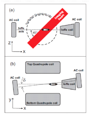
Figure 1: Scheme of the main components composing the magnetic trap and the additional extra coils producing the necessary oscillatory fields generating trapped quantum turbulence.

Small amplitudes of oscillation can only produce a bending mode intrinsically connected to the scissor mode [130] present in atomic trapped superfluids. Larger amplitudes of oscillation, combined with longer excitation times, can produce vortices with a characteristic array of QT. As is shown in Fig. 2, in a range of the excitation parameters, there arise vortices directed along the cloud axis, but still not yet showing a fully tangled configuration. Quantum turbulence takes place in the region of parameters with a clear separation of behavior between the regions.

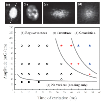
Figure 2: Diagram, on the excitation amplitude-time plane, showing the observed characteristic regions of four different identifiable structures, from the simple bending of the superfluid axis, to the creation of vortices, vortex tangle, and to granulation.

The generation of vortices takes place because the oscillation of the atomic superfluid cloud produces collective modes [112] leading to the generation of coherent modes [35]. In a more recent observation, it has been verified [131] that the excitation, through a combination of oscillations produces, together with collective modes, the excitation of the second sound mode coupled to the dipole mode. This excitation corresponds to the counterflow between condensate and thermal cloud, with the possible generation of vortices in the regions of the maximal relative motion. At low temperatures, when the normal fraction is negligible, dynamic instability appears due to the counterflow between different parts of the condensate [81, 82, 83, 84, 85, 86, 87, 88].

Being generated, vortices can be distributed in many directions, first, without actually forming a tangled configuration. When the finite size of the cloud is saturated with the vortices, any further pumped energy forces a fast evolution of the vortices, promoting their reactions by reconnections [132], eventually yielding a turbulent cloud. At this stage, not only the distribution of the vortices is an indication for the occurrence of turbulence, but also a change in the hydrodynamic behavior, during the free expansion of the cloud, works as the indicator of turbulence. While a non-turbulent cloud of an atomic superfluid demonstrates the inversion of aspect ratio during free expansion, the turbulent cloud preserves the original aspect ratio [111, 133].

It has been observed that the existence of a boundary, between the regular and turbulent superfluids, on the amplitude-time diagram of Fig. 2 is the consequence of the finite size of the cloud, as explained in Ref. [113].

For the extreme case of excitation (high amplitude and longer excitation times), the turbulent condensate evolves into a granulated state, when the original condensate cloud breaks into many grains. The transition from the turbulent to fragmented cloud is presented by the density profile of Fig. 3.

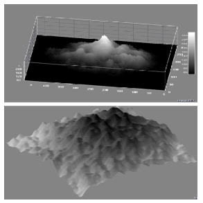
Figure 3: The difference between a turbulent and a granulated cloud. While in the first case the landscape is made of vortex filaments distributed in space, the granulated state corresponds to a collection of grains characterizing strong density fluctuations.

The experimental observation of the atomic cloud inside the trap is not easy. This is because the produced condensate has the size of just a few microns. To perform an absorption measurement in situ, we would be severely limited by diffraction. We therefore, first, allow a free expansion of the cloud, and then perform absorption measurements. For the observed states, discussed above, the time of flight before absorption was of 15 ms. In this case, the size of the cloud is many times larger than the actual size in situ. As far as, during the time of flight, the density is greatly reduced, the interactions are also reduced, freezing the existent structure, that now evolves much slower in time. It is a general consensus that the free expansion preserves the in situ structure of the atomic cloud.

Figure 4 demonstrates the absorption image of the granulated cloud and the details showing the domains of the grains after free expansion of 15 ms. We observe an isotropic expansion and the details of the figure allow us to identify the grains arising in the originally homogeneous superfluid. Applying the reversibility analysis, we find that, in situ, the grains have the average size of about 0.25 microns. They are clearly not regular either in shape or in size and do not form any structure that could be observed through the absorption.

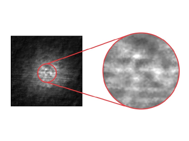
Figure 4: Absorption by the granulated cloud showing the domains of the grains

For convenience, let us summarize the data characteristic of our experiments with ⁸⁷Rb atoms. The mass of a Rb atom is $m=1.445\times 10^{-22}$ g. The scattering length is $a_{s}=0.577\times 10^{-6}$ cm. The radial frequency is $\omega_{\perp}=1.32\times 10^{3}$ s^-1 and longitudinal frequency is $\omega_{z}=1.445\times 10^{2}$ s^-1. The corresponding oscillator lengths are $l_{\perp}=0.744\times 10^{-4}$ cm and $l_{z}=2.248\times 10^{-4}$ cm. The average oscillator frequency and length are $\omega_{0}=0.631\times 10^{3}$ s^-1 and $l_{0}=1.076\times 10^{-4}$ cm. The effective condensate volume is $V_{eff}=0.783\times 10^{-11}$ cm³. The average condensate density is $\rho\sim 2.554\times 10^{15}$ cm^-3. The mean interatomic distance is $a=0.732\times 10^{-5}$ cm, which is much larger than the scattering length. Hence, the gas is rarified. The gas parameters are small, $\rho a_{s}^{3}=0.491\times 10^{-3}$ and $\rho^{1/3}a_{s}=0.079$. This implies that atomic interactions are weak. However, the effective coupling parameter (44) is large, $g=1.95\times 10^{4}$. Therefore the corresponding nonlinearity is very large.

The trap is subject to an external field modulation during the time $t_{ext}=0.02-0.06$ s, with an alternating potential of frequency $\omega=1.257\times 10^{3}$ s^-1. The related modulation period is $t_{mod}\equiv 2\pi/\omega=5\times 10^{-3}$ s. The local equilibration time is $t_{loc}=m/(\hbar\rho a_{s})=0.929\times 10^{-4}$ s. This is much shorter than the modulation period, because of which the system is always in local equilibrium.

With the average grain size $l_{g}\sim 2.5\times 10^{-5}$ cm, the number of atoms inside a grain is $(l_{g}/a)^{3}\sim 40$. And the number of grains in the trap is of order $(l_{0}/l_{g})^{3}\sim 400$.

The majority of experimental observations can be explained by the models of Secs. 4 to 7. But, certainly, other experiments for cross-checking the measured and theoretical dependencies are needed. Recent measurements of the momentum distribution of a turbulent cloud show the existence of a power-law type dependence $n(k)\propto k^{-\delta}$, which also requires confirmation and analysis with respect to its relation to the Kolmogorov-type behavior.

11 Conclusion

We have described the procedure of exciting a system of trapped Bose-condensed atoms by an external alternating potential, forcing the system to pass through several qualitatively different stages. Initially, the system is almost completely condensed, which is characterized by the broken global gauge symmetry. Applying sufficiently strong external perturbation transfers the system into a nonequilibrium state. First, there appear separate vortices and antivortices, which marks the transfer from the regular superfluid to vortex superfluid. Increasing perturbations is realized by either strengthening the amplitude of the applied alternating field or by its longer action on the system. Sufficiently strong perturbation generates a variety of coherent topological modes that decay into basic vortices with vorticity one. Thus, a multiplicity of vortices and antivortices is effectively generated. The location of these vortices inside the trap and their directions are random, which is caused by the absence of a unique rotation axis of the applied alternating potential. Because of this, the increasing perturbation creates not a vortex lattice, as it would be in the case of a uniaxial rotation, but forms en ensemble of randomly directed vortices. When the number of vortices becomes large, they form a random vortex tangle typical of quantum turbulence. Increasing further the amount of energy, injected into the trap, breaks the system into pieces. Then Bose-condensed grains, or droplets, are surrounded by uncondensed gas in the normal state. Pumping more energy into the trap reduces the fraction of condensed atoms. Finally, the system should transfer into the normal state, where the global gauge symmetry is restored.

Thus, starting with a regular superfluid, we pass through the states of vortex superfluid, turbulent superfluid, granular fluid, and should finish with chaotic fluid that is in a state of classical turbulence. In that way, the initial state with global gauge symmetry breaking is transformed, through a sequence of qualitatively different regimes, to a state with the restored global gauge symmetry. Transitions between different regimes are classified as crossovers, though they are sufficiently sharp for allowing us to define the corresponding crossover lines. All these transitions, except that to chaotic fluid, are illustrated by experiments with trapped ⁸⁷Rb atoms.

Acknowledgement

We are grateful to all our co-authors for collaboration. One of the authors (V.I.Y.) acknowledges financial support from the Russian Foundation for Basic Research.

References

- [1] L.D. Landau and E.M. Lifshitz, Statistical Physics (Pergamon, Oxford, 1980).
- [2] V.I. Yukalov and A.S. Shumovsky, Lectures on Phase Transitions (World Scientific, Singapore, 1990).
- [3] D. Sornette, Critical Phenomena in Natural Sciences (Springer, Berlin, 2006).
- [4] A. Polkovnikov, K. Sengupta, A. Silva, and M. Vengalatore, Rev. Mod. Phys. 83, 863 (2011).
- [5] L. Pitaevskii and S. Stringari, Bose-Einstein Condensation (Clarendon, Oxford, 2003).
- [6] E.H. Lieb, R. Seiringer, J.P. Solovej, and J. Yngvason, The Mathematics of the Bose Gas and Its Condensation (Birkhauser, Basel, 2005).
- [7] V. Letokhov, Laser Control of Atoms and Molecules (Oxford University, New York, 2007).
- [8] C.J. Pethik and H. Smith, Bose-Einstein Condensation in Dilute Gases (Cambridge University, Cambridge, 2008).
- [9] P.W. Courteille, V.S. Bagnato, and V.I. Yukalov, Laser Phys. 11, 659 (2001).
- [10] J.O. Andersen, Rev. Mod. Phys. 76, 599 (2004).
- [11] V.I. Yukalov, Laser Phys. Lett. 1, 435 (2004).
- [12] K. Bongs and K. Sengstock, Rep. Prog. Phys. 67, 907 (2004).
- [13] V.I. Yukalov and M.D. Girardeau, Laser Phys. Lett. 2, 375 (2005).
- [14] A. Posazhennikova, Rev. Mod. Phys. 78, 1111 (2006).
- [15] V.I. Yukalov, Laser Phys. Lett. 4, 632 (2007).
- [16] N.P. Proukakis and B. Jackson, J. Phys. B 41, 203002 (2008).
- [17] V.A. Yurovsky, M. Olshanii, and D.S. Weiss, Adv. At. Mol. Opt. Phys. 55, 61 (2008).
- [18] V.I. Yukalov, Laser Phys. 19, 1 (2009).
- [19] A.L. Fetter, Rev. Mod. Phys. 81, 647 (2009).
- [20] V.I. Yukalov, Phys. Part. Nucl. 42, 460 (2011).
- [21] N.N. Bogolubov, Lectures on Quantum Statistics (Gordon and Breach, New York, 1967), Vol. 1.
- [22] N.N. Bogolubov, Lectures on Quantum Statistics (Gordon and Breach, New York, 1970), Vol. 2.
- [23] V.I. Yukalov, Phys. Rep. 208, 395 (1991).
- [24] V.I. Yukalov, Int. J. Mod. Phys. 21, 69 (2007).
- [25] V.I. Yukalov, Ann. Phys. (N.Y.) 323, 461 (2008).
- [26] V.I. Yukalov, Phys. Lett. A 375, 2797 (2011).
- [27] E.P. Gross, Phys. Rev. 106, 161 (1957).
- [28] E.P. Gross, Ann. Phys. (N.Y.) 4, 57 (1958).
- [29] V.L. Ginzburg and L.P. Pitaevskii, J. Exp. Theor. Phys. 7, 858 (1958).
- [30] E.P. Gross, Nuovo Cimento 20, 454 (1961).
- [31] L.P. Pitaevskii, J. Exp. Theor. Phys. 13, 451 (1961).
- [32] B.A. Malomed, Soliton Management in Periodic Systems (Springer, New York, 2006).
- [33] Y.V. Kartashov, B.A. Malomed, and L. Torner, Rev. Mod. Phys. 83, 247 (2011).
- [34] J.R. Klauder and B.S. Skagerstam, Coherent States (World Scientific, Singapore, 1985).
- [35] V.I. Yukalov, E.P. Yukalova, and V.S. Bagnato, Phys. Rev. A 56, 4845 (1997).
- [36] V.I. Yukalov, E.P. Yukalova, and V.S. Bagnato, Laser Phys. 10, 26 (2000).
- [37] E.A. Ostrovskaya, Y.S. Kivshar, M. Lisak, B. Hall, F. Cattani, and D. Anderson, Phys. Rev. A 61, 031601 (2000).
- [38] D.L. Feder, M.S. Pindzola, L.A. Collins, B.I. Schneider, and C.W. Clark, Phys. Rev. A 62, 053606 (2000).
- [39] V.I. Yukalov, E.P. Yukalova, and V.S. Bagnato, Laser Phys. 11, 455 (2001).
- [40] Y.S. Kivshar, T.J. Alexander, and S.K. Turitsin, Phys. Lett. A 278, 225 (2001).
- [41] R. D’Agosta, B.A. Malomed, and C. Presilla, Laser Phys. 12, 37 (2002).
- [42] V.I. Yukalov, E.P. Yukalova, and V.S. Bagnato, Laser Phys. 12, 231 (2002).
- [43] V.I. Yukalov, E.P. Yukalova, and V.S. Bagnato, Laser Phys. 12, 1325 (2002).
- [44] B. Damski, Z.P. Karkuszewski, K. Sasha, and J. Zakrzewski, Phys. Rev. A 65, 013604 (2002).
- [45] R. D’Agosta and C. Presilla, Phys. Rev. A 65, 043609 (2002).
- [46] V.I. Yukalov, E.P. Yukalova, and V.S. Bagnato, Phys. Rev. A 66, 043602 (2002).
- [47] N.P. Proukakis and P. Lambropoulos, Eur. Phys. J. D 19, 355 (2002).
- [48] V.I. Yukalov, E.P. Yukalova, and V.S. Bagnato, Laser Phys. 13, 551 (2003).
- [49] V.I. Yukalov, E.P. Yukalova, and V.S. Bagnato, Laser Phys. 13, 861 (2003).
- [50] S.K. Adhikari, Phys. Lett. A 308, 302 (2003).
- [51] S.K. Adhikari, J. Phys. B 36, 1109 (2003).
- [52] P. Muruganandam and S.K. Adhikari, J. Phys. B 36, 2501 (2003).
- [53] V.I. Yukalov, K.P. Marzlin, and E.P. Yukalova, Laser Phys. 14, 565 (2004).
- [54] V.I. Yukalov, K.P. Marzlin, and E.P. Yukalova, Phys. Rev. A 69, 023620 (2004).
- [55] S.K. Adhikari, Phys. Rev. A 69, 063613 (2004).
- [56] V.S. Filho, L. Tomio, A. Gammal, and T. Frederico, Phys. Lett. A 325, 420 (2004).
- [57] E.R. Ramos, L. Sanz, V.I. Yukalov, and V.S. Bagnato, Phys. Lett. A 365, 126 (2007).
- [58] E.R. Ramos, L. Sanz, V.I. Yukalov, and V.S. Bagnato, Phys. Rev. A 76, 033608 (2007).
- [59] E.R. Ramos, L. Sanz, V.I. Yukalov, and V.S. Bagnato, Nucl. Phys. 790, 776 (2007).
- [60] E.R. Ramos, E.A. Henn, J.A. Seman, M.A. Caracanhas, K.M. Magalhães, K. Helmerson, V.I. Yukalov, and V.S. Bagnato, Phys. Rev. A 78, 063412 (2008).
- [61] V.I. Yukalov and V.S. Bagnato, Laser Phys. Lett. 6, 399 (2009).
- [62] J. Williams, R. Walser, J. Cooper, E.A. Cornell, and M. Holland, Phys. Rev. A 61, 063612 (2000).
- [63] V.I. Yukalov, Laser Phys. Lett. 3, 406 (2006).
- [64] V.I. Yukalov, Moscow Univ. Phys. Bull. 31, 10 (1976).
- [65] V.I. Yukalov, J. Math. Phys. 32, 1235 (1991).
- [66] V.I. Yukalov and E.P. Yukalova, Ann. Phys. (N.Y.) 277, 219 (1999).
- [67] V.I. Yukalov and E.P. Yukalova, Chaos. Solit. Fract. 14, 839 (2002).
- [68] N.N. Bogolubov and Y.A. Mitroposlky, Asymptotic Methods in the Theory of Nonlinear Oscillations (Gordon and Breach, New York, 1961).
- [69] V.I. Yukalov and E.P. Yukalova, Phys. Part. Nucl. 31, 561 (2000).
- [70] V.I. Yukalov and E.P. Yukalova, Phys. Part. Nucl. 35, 348 (2004).
- [71] A. Smerzi, S. Fantoni, S. Giovanazzi, and S.R. Shenoy, Phys. Rev. Lett. 79, 4950 (1997).
- [72] V.I. Yukalov, Mod. Phys. Lett. B 17, 95 (2003).
- [73] V.I. Yukalov and E.P. Yukalova, Laser Phys. 16, 354 (2006).
- [74] V.I. Yukalov and E.P. Yukalova, Phys. Rev. A 73, 022335 (2006).
- [75] V.I. Yukalov and E.P. Yukalova, J. Phys. Conf. Ser. 104, 012003 (2008).
- [76] B. Baizakov, G. Filatrella, B. Malomed, and M. Salerno, Phys. Rev. E 71, 036619 (2005).
- [77] E.J. Yarmchuk, M.J. Gordon, and R.E. Packard, Phys. Rev. Lett. 43, 214 (1979).
- [78] M.R. Matthews, B.P. Anderson, P.C. Haljan, D.S. Hall, C.E. Wieman, and E.A. Cornell, Phys. Rev. Lett. 83, 2498 (1999).
- [79] K.W. Madison, F. Chevy, W. Wohlleben, and J. Dalibard, Phys. Rev. Lett. 84, 806 (2000).
- [80] P. Rosenbusch, V. Bretin, and J. Dalibard, Phys. Rev. Lett. 89, 200403 (2002).
- [81] V.I. Yukalov, Acta Phys. Pol. A 57, 295 (1980).
- [82] Z. Dutton, M. Budde, C. Slowe, and L.V. Hau, Science 293, 663 (2001).
- [83] V.I. Yukalov and E.P. Yukalova, Laser Phys. Lett. 1, 50 (2004).
- [84] J. Ruostekoski and Z. Dutton, Phys. Rev. A 72, 063626 (2005).
- [85] I. Shomroni, E. Lahoud, S. Levy, and J. Steinhauer, Nature Phys. 5, 193 (2009).
- [86] M. Ma, R. Carretero-Gonzalez, P.G. Kevrekidis, D.J. Frantzeskakis, and B.A. Malomed, Phys. Rev. A 82, 023621 (2010).
- [87] S. Ishiro, M. Tsubota, and H. Takeuchi, Phys. Rev. A 83, 063602 (2011).
- [88] T.P. Simula, Phys. Rev. A 84, 021603 (2011).
- [89] J.R. Abo-Shaeer, C. Raman, J.M. Vogels, and W. Ketterle, Science 292, 476 (2001).
- [90] E.A.L. Henn, J.A. Seman, E.R.F. Ramos, M. Caracanhas, P. Castilho, E.P. Olimpio, G. Roati, D.V. Magalhães, K.M.F. Magalhães, and V.S. Bagnato, Phys. Rev. A 79, 043618 (2009).
- [91] J.A. Seman, E.A.L. Henn, M. Haque, R.F. Shiozaki1, E.R.F. Ramos, M. Caracanhas, P. Castilho, C. Castelo Branco, P.E.S. Tavares, F.J. Poveda-Cuevas, G. Roati, K.M.F. Magalhães, and V.S. Bagnato, Phys. Rev. A 82, 033616 (2010).
- [92] J.A. Seman, Thesis (University of São Paulo, São Carlos, 2011).
- [93] R.P. Feynman, Prog. Low Temp. Phys. 1, 17 (1955).
- [94] P.A. Davidson, Turbulence: Introduction for Scientists and Engineers (Oxford University, Oxford, 2004).
- [95] R. Donnelly and C. Swanson, J. Fluid Mech. 173, 387 (1986).
- [96] A.N. Kolmogorov, Proc. USSR Acad Sci. 30, 299 (1941).
- [97] A.N. Kolmogorov, Proc. USSR Acad Sci. 32, 16 (1941).
- [98] K. Sreenivasan, Phys. Fluids 7, 2778 (1995).
- [99] H.E. Hall and W.F. Vinen, Proc. Roy. Soc. London A 238, 204 (1956).
- [100] W.F. Vinen, Proc. Roy. Soc. London A 243, 400 (1958).
- [101] J. Maurer and P. Tabeling, Eur. Phys. Lett. 43, 29 (1998).
- [102] S.R. Stalp, L. Skrbek, and R.J. Donnelly, Phys. Rev. Lett. 82, 4831 (1999).
- [103] B.V. Svistunov, Phys. Rev. B 52, 3647 (1995).
- [104] M. Kobayashi and M. Tsubota, J. Phys. Soc. Jpn. 74, 3248 (2005).
- [105] C.F. Barenghi, R.J. Donnelly, and W.F. Vinen, Quantized Vortex Dynamics and Superfluid Turbulence (Springer, New York, 2001).
- [106] W.F. Vinen and J.J. Niemela, J. Low Temp. Phys. 128, 167 (2002).
- [107] V.I. Yukalov, Laser Phys. Lett. 7, 467 (2010).
- [108] B. Nowak, J. Schole, D. Sexty, and T. Gasenzer, Phys. Rev. A 85, 043627 (2012).
- [109] M. Kobayashi and M. Tsubota, Phys. Rev. A 76, 045603 (2007)
- [110] M. Tsubota, J. Phys. Condens. Matt. 21, 164207 (2009).
- [111] E.A.L. Henn, J.A. Seman, G. Roati, K.M.F. Magalhães, and V.S. Bagnato, Phys. Rev. Lett. 103, 045301 (2009).
- [112] J.A. Seman, R.F. Shiozaki, F.J. Poveda-Cuevas, E.A.L. Henn, K.M.F. Magalhães, G. Roati, G.D. Telles, and V.S. Bagnato, J. Phys. Conf. Ser. 264, 012004 (2011).
- [113] R.F. Shiozaki, G.D. Telles, V.I. Yukalov, and V.S. Bagnato, Laser Phys. Lett. 8, 393 (2011).
- [114] J.A. Seman, E.A.L. Henn, R.F. Shiozaki, G. Roati, F.J. Poveda-Cuevas, K.M.F. Magalhães, V.I. Yukalov, M. Tsubota, M. Kobayashi, K. Kasamatsu, and V.S. Bagnato, Laser Phys. Lett. 8, 691 (2011).
- [115] V.I. Yukalov, E.P. Yukalova, and V.S. Bagnato, Laser Phys. 19, 686 (2009).
- [116] R. Graham and A. Pelster, Int. J. Bifurc. Chaos. 19, 2745 (2009).
- [117] C. Gaul and C.A. Müller, Phys. Rev. A 83, 063629 (2011).
- [118] V.I. Yukalov and R. Graham, Phys. Rev. A 75, 023619 (2007).
- [119] V.I. Yukalov, E.P. Yukalova, K.V. Krutitsky, and R. Graham, Phys. Rev. A 76, 053623 (2007).
- [120] V.I. Yukalov, Int. J. Mod. Phys. 17, 2333 (2003).
- [121] V.I. Yukalov and E.P. Yukalova, Laser Phys. 21, 1448 (2011).
- [122] V.N. Tsytovich, Theory of Turbulent Plasma (Consultant Bureau, New York, 1977).
- [123] S. Dyachenko, A.C. Newell, A. Pushkarev, and V.E. Zakharov, Physica D 57, 96 (1992).
- [124] S. Galtier, S.N. Nazarenko, A.C. Newell, and A. Pouquet, J. Plasma Phys. 63, 447 (2000).
- [125] N.G. Berloff and B.V. Svistunov, Phys. Rev. A 66, 013603 (2002).
- [126] Y. Lvov, S. Nazarenko, and R. West, Physica D 184, 333 (2003).
- [127] V. Zakharov, F. Dias, and A. Pushkarev, Phys. Rep. 398,1 (2004).
- [128] C. Raman, Phys. Rev. Lett. 87, 210402 (2001).
- [129] K.W. Madison, F. Chevy, W. Wohlleben, and J. Dalibard, J. Mod. Opt. 47, 2715 (2000).
- [130] O.M. Marago, S.A. Hopkins, J. Arlt, E. Hodby, G. Hechenblaikner, and C.J. Foot, Phys. Rev. Lett. 84, 2056 (2000).
- [131] P.E.S. Tavares, Thesis (University of São Paulo, São Carlos, 2011).
- [132] M. Tsubota, S.I. Ogawa, and Y. Hattori, J. Low Temp. Phys. 121, 435 (2000).
- [133] M. Caracanhas, A.L. Fetter, S.R. Muniz, K.M.F. Magalhães, G. Roati, G. Bagnato, and V.S. Bagnato, J. Low Temp. Phys. 166, 49 (2012).