Yangian symmetric correlators

D. Chicherin^ab and R. Kirschner^c

• St. Petersburg Department of Steklov Mathematical Institute of Russian Academy of Sciences, Fontanka 27, 191023 St. Petersburg, Russia

• Chebyshev Laboratory, St.-Petersburg State University,
  14th Line, 29b, Saint-Petersburg, 199178 Russia

• Institut für Theoretische Physik, Universität Leipzig,
  PF 100 920, D-04009 Leipzig, Germany

Similarity transformations and eigenvalue relations of monodromy operators composed of Jordan-Schwinger type $\mathrm{L}$ matrices are considered and used to define Yangian symmetric correlators of $n$-dimensional theories. Explicit expressions are obtained and relations are formulated. In this way basic notions of the Quantum inverse scattering method provide a convenient formulation for high symmetry and integrability not only in lower dimensions.

1 Construction scheme and motivations

We consider $N$-point correlators in $n$ dimensions, i.e. functions of $nN$ variables interpreted as $N$ points $\mathbf{x}_{i}$ with coordinates $\left(x_{a,i}\right)_{a=1}^{n}=\left(x_{1,i},x_{2,i},\cdots,x_{n,i}\right)$. Associated with these coordinates we shall work with $nN$ Heisenberg canonical pairs $\mathbf{p}_{i}=\left(p_{a,i}\right)_{a=1}^{n}=\left(p_{1,i},p_{2,i},\cdots,p_{n,i}\right)$ and $\mathbf{x}_{i}=\left(x_{a,i}\right)_{a=1}^{n}=\left(x_{1,i},x_{2,i},\cdots,x_{n,i}\right)$, $[p_{a,i},x_{b,j}]=\delta_{a,b}\delta_{i,j}$. We consider the partition of the index set $N=\{1,2,\cdots,N\}$ labeling these points in two non-overlapping subsets $I$ and $J$, $I\cup J=N,\,I\cap J=\varnothing$. The partition of the set of $N$ sites into the subsets $I,J$ can also be denoted as signature, i.e. by a sequence of symbols ${}^{\prime\prime}+^{\prime\prime},\,^{\prime\prime}-^{\prime\prime}$ where the symbol ${}^{\prime\prime}+^{\prime\prime}$ is put for a site in $I$ and ${}^{\prime\prime}-^{\prime\prime}$ for a site in $J$.

We define the action of $g\ell_{n}$ on the points in dependence of their signature as

$$\delta x_{c,i}=\left[\left[\mathrm{L}^{+}_{i}\right]_{a,b},\ x_{c,i}\right],\ i\in I,\ \ \ \delta x_{c,j}=\left[\left[\mathrm{L}^{-}_{j}\right]_{a,b},x_{c,j}\right],\ j\in J$$

$$\left[\mathrm{L}^{+}_{i}\right]_{a,b}=p_{a,i}x_{b,i}\;,\;\;\;\left[\mathrm{L}^{-}_{j}\right]_{a,b}=-x_{a,j}p_{b,j}\,.$$ (1.1)

We denote the inner product by $(\,\cdot\,)$,

$$(ji)\equiv(ij)\equiv(\mathbf{x}_{i}\cdot\mathbf{x}_{j})\equiv x_{a,i}x_{a,j}\,.$$ (1.2)

and notice that for $i\in I,j\in J$ it is $g\ell_{n}$ invariant in the sense

$$[\mathrm{L}^{+}_{i}+\mathrm{L}^{-}_{j},(\mathbf{x}_{i}\cdot\mathbf{x}_{j})]=0\,.$$

Monomials of the form

$$\Phi_{I,J}=\prod_{i\in I,j\in J}(\mathbf{x}_{i}\cdot\mathbf{x}_{j})^{\lambda_{ij}}$$ (1.3)

are $g\ell_{n}$ invariant and general $g\ell_{n}$ invariant correlators are superpositions of such monomials with varying exponents which can take complex values. In general the coordinates are complex valued.

Note that the the inner product results in an invariant if the coordinates of the involved points $\mathbf{x}_{i},\mathbf{x}_{j}$ transform differently, one by $\mathrm{L}^{+}$ the other by $\mathrm{L}^{-}$. This is the formal reason for considering the two actions on coordinates and for introducing the signature for distinction. In applications to scattering amplitudes this is related to gluon helicity.

We add the remark that the case $n=2$ is special because there is the additional invariance relation involving the symplectic form

$$x_{1,k}x_{2,l}-x_{2,k}x_{1,l}=(\mathbf{x}_{k}\mathbf{\cdot\varepsilon}\mathbf{x}_{l}),$$ (1.4)

$$[\mathrm{L}^{\pm}_{k}+\mathrm{L}^{\pm}_{l},(\mathbf{x}_{k}\mathbf{\cdot\varepsilon}\mathbf{x}_{l})]=\pm(\mathbf{x}_{k}\mathbf{\cdot\varepsilon}\mathbf{x}_{l})\ \mathrm{I}.$$

This implies that in this case the invariant correlators depend in general both on the inner products (1.2) and on the symplectic products (1.4).

The trace of the matrix $\mathrm{L}^{\pm}_{k}$ is $(\mathbf{x}_{k}\cdot\mathbf{p}_{k})+n$ or $-(\mathbf{x}_{k}\cdot\mathbf{p}_{k})$. It commutes with all the matrix elements and generates the $u(1)$ subalgebra in $g\ell_{n}$ acting as infinitesimal dilatations on the coordinates. Let us restrict the discussion to correlators of definite weights, i.e. eigenfunctions of all the $N$ dilatation operators $(\mathbf{x}_{k}\cdot\mathbf{p}_{k})$, $k=1,\cdots,N$. The monomial (1.3) has dilatation weights $\sum_{j\in J}\lambda_{ij}$ for $i\in I$ and $\sum_{i\in I}\lambda_{ij}$ for $j\in J$ and a generic $g\ell_{n}$ invariant correlator with these weights is given by this monomial multiplied with a function of the cross ratios

$$X_{ij,kl}=\frac{(ij)(kl)}{(il)(kj)}\,,\,\,\,\,i,k\in I\,,\,\,\,\,j,l\in J\,.$$

By the restriction to correlators of definite weights at all points the $n$ dimensional space reduces to the corresponding projective space.

Along with the $N$ point correlator we consider the quantum spin chain of $N$ sites with the states at site $k$ forming a representation of $g\ell_{n}$ of Jordan-Schwinger type [1, 2, 3, 4, 5, 6, 7, 8, 15, 14]. This representation is spanned by monomials in the coordinates of the point $\mathbf{x}_{k}$ with the eigenvalue of the action of $(\mathbf{x}_{k}\cdot\mathbf{p}_{k})$ coinciding with the weight of the correlator at this point. $(\mathrm{L}^{\pm}_{k})_{a,b}$ are the generators of this representation in dependence on the signature. The weight characterizes the representation which is irreducible for generic values.

The $\mathrm{L}$ matrices are defined in terms these generator matrices by adding a spectral parameter being a complex number,

$$\mathrm{L}^{+}_{k}(u_{k})=u_{k}+\mathbf{p}_{k}\mathbf{x}_{k}\;,\;\;\;\mathrm{L}^{-}_{k}(u_{k})=u_{k}-\mathbf{x}_{k}\mathbf{p}_{k}\,,$$ (1.5)

or in component form

$$\left[\mathrm{L}^{+}_{k}(u_{k})\right]_{a,b}=u_{k}\delta_{a,b}+p_{a,k}x_{b,k}\;,\;\;\;\left[\mathrm{L}^{-}_{k}(u_{k})\right]_{a,b}=u_{k}\delta_{a,b}-x_{a,k}p_{b,k}\,.$$ (1.6)

In our notations (1.5) we omit a symbol of tensor product $\otimes$ for short. Notations like $\mathbf{x}_{i}\mathbf{x}_{j}$ (for example in the definition (1.5)) are not to be confused with the inner product (1.2).

Both operators $\mathrm{L}^{\pm}(u)$ respect the $\mathcal{R}\mathrm{LL}$-relation with Yang’s $\mathcal{R}$-matrix,

$$\mathcal{R}_{ab,ef}(u-v)\,\mathrm{L}_{ec}(u)\,\mathrm{L}_{fd}(v)=\mathrm{L}_{bf}(v)\,\mathrm{L}_{ae}(u)\,\mathcal{R}_{ef,cd}(u-v),$$ (1.7)

where $a,b,\cdots=1,\cdots,n$ and $\mathcal{R}_{ab,cd}(u)=u\,\delta_{ac}\,\delta_{bd}+\delta_{ad}\,\delta_{bc}.$ This equation also referred to as the fundamental commutation relation contains in a compact form all relations of the underlying Yangian symmetry algebra $Y(g\ell_{n})$. The $\mathrm{L}$ matrices are well known as the basic tool of treating the spin chain by the Quantum Inverse Scattering Method (QISM) [24, 25, 28, 29].

In the present paper we are going to study symmetry conditions on correlators going beyond the mentioned $g\ell_{n}$ invariance to be formulated in terms of the $\mathrm{L}$ matrices. For this aim we write down the monodromy matrix related to the chain as the ordered product of $\mathrm{L}^{\pm}$-operators (1.5) each refering to one of the sites,

$$\mathrm{T}^{\alpha_{1}\cdots\alpha_{N}}_{1\cdots N}(u_{1},\cdots,u_{N})=\mathrm{L}^{\alpha_{1}}_{1}(u_{1})\mathrm{L}^{\alpha_{2}}_{2}(u_{2})\cdots\mathrm{L}^{\alpha_{N}}_{N}(u_{N})\,,$$ (1.8)

where $\alpha_{1}\alpha_{2}\cdots\alpha_{N}$ denotes the signature, i.e. $\alpha_{k}=\pm$ at $k=1,\cdots,N$. The lower indices refer to the chains site with the representation (the quantum space) where the operators act nontrivially. We will omit supplementary indices when it does not lead to misunderstandings.

We intend to study the similarity transformation of the monodromy matrix (1.8) by invariant correlators like (1.3). We shall write the result of the similarity transformation by (1.3) in terms of the monodromy matrix with changed spectral parameters plus a remainder

$$\Phi\circ\mathrm{T}(u_{1},\cdots,u_{N})\equiv\Phi^{-1}\mathrm{T}(u_{1},\cdots,u_{N})\,\Phi=\mathrm{T}(u_{1}^{\prime},\cdots,u_{N}^{\prime})+\hat{r}\,.$$ (1.9)

Some remainder terms vanish at special values of the exponents $\lambda_{ij}$ (1.3). Here we adopt the notation $\Phi\circ\mathrm{T}\equiv\Phi^{-1}\mathrm{T}\,\Phi$.

Solutions of the following eigenvalue relations for the monodromy matrix can be obtained from such similarity relations,

$$\mathrm{T}(u_{1},\cdots,u_{N})\cdot\Phi(u_{1},\cdots,u_{N})=E(u_{1},\cdots,u_{N})\,\Phi(u_{1},\cdots,u_{N})\,.$$ (1.10)

Here the matrix $\mathrm{T}$ with operator elements acts on the correlator function resulting in the r.h.s proportional to the unit matrix.

Indeed, by acting with both sides of (1.9) on the basic state which is represented by a constant function of the variables $\mathbf{x}_{1},\cdots,\mathbf{x}_{N}$ and by requiring the vanishing of the remainder up to a constant,

$$\hat{r}\cdot 1=\eta$$

by choice of parameters $\lambda_{ij}$ we arrive at the above eigenvalue relation with

$$E(u_{1},\cdots,u_{N})=\mathrm{T}(u_{1}^{\prime},\cdots,u_{N}^{\prime})\cdot 1+\eta=\prod_{I,J}(u_{i}^{\prime}+1)u_{j}^{\prime}+\eta$$ (1.11)

where we take into account that $\mathrm{L}^{+}(u)\cdot 1=u+1$ and $\mathrm{L}^{-}(u)\cdot 1=u$ (1.5).

The eigenvalue relation (1.10) provides the formulation of the extended symmetry condition on the correlators to be studied here. A Yangian symmetric correlator is defined as a $g\ell_{n}$ invariant correlator of definite dilatation weights being a solution of (1.10).

In the present paper we focus on regular correlators not involving distributions. The symmetric correlator can be represented graphically by drawing the chain with its sites $k$, marked by the corresponding spectral parameter $u_{k}$, dilatation weight $2\ell_{k}$ and signature $\pm$, and with lines (links) connecting sites $i,j$ of different signature, provided the dependence on the corresponding $g\ell_{n}$ invariant $(\mathbf{x}_{i}\cdot\mathbf{x}_{j})$ is non-trivial. Otherwise the corresponding line is omitted. In this way we distinguish symmetric correlators corresponding to more or less connected or even disconnected graphs.

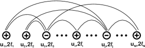
Figure 1: Graph representing a symmetric correlator

According to the above remark in the special case $n=2$ another type of links between sites of the same signature exist. The special features of this case will not be considered here.

Actually this case is well known because here the reduction to $s\ell(2)$ can be done in such a way that the inner products $(\mathbf{x}_{i}\cdot\mathbf{x}_{j})$ and also the symplectic products $(\mathbf{x}_{k}\mathbf{\varepsilon}\cdot\mathbf{x}_{l})$ turn into differences in coordinate ratios and that the Möbius transformations of those ratios are generated. Symmetric correlators appear e.g. in QCD as (holomorphic part of) kernels of BFKL equations [21] of perturbative Regge asymptotics or of DGLAP/ERBL equations [19, 20] of Bjorken asymptotics. In the latter case they also generate the anomalous dimensions of composite operators built of light-cone components of fields and their derivatives.

The solution of Yang-Baxter $\mathrm{RLL}$ relations by solving the Yangian conditions on the corresponding kernel (4-point correlator) has been discussed in [22].

The case $n=4$ is related to conformal symmetry in 4 dimensional field theory. The supersymmetric extension $n=4|4$ can be formulated in a straightforward way. Symmetric correlators appear here as kernels of the renormalization scale dilatation operator or as perturbative scattering amplitudes in twistor representation.

The observation of the dual conformal and Yangian symmetry of super Yang-Mills amplitudes attracted great attention [9, 11, 10]. The extended symmetries became new ingredients of the modern tools of amplitude calculations and provide new insight into the intrinsic structure of gauge theories and their relation to strings.

The relation of Yang-Mills amplitudes to kernels of Yang-Baxter operators has been observed in [12] indicating also the potential role of spectral parameters for regularization of IR divergent loop integrals. The present approach to Yangian symmetric correlators has been applied to super Yang-Mills scattering amplitudes in [13].

The notion of Yangian algebra was introduced by Drinfeld [23] in general form. The case related to $g\ell_{n}$ was worked out earlier by L. Faddeev and collaborators [24, 25, 26] in the QISM formulation. The relation of the latter formulation to the one in algebra generators by Drinfeld is well explained in [27]. In the papers discussing the Yangian symmetry of SYM amplitudes, e.g. [9] the algebra generator form is preferred. We use here the advantages of the QISM form.

The plan of the paper is as follows. In Section 2 we apply the general scheme outlined above to construct all $2$- and $3$-point symmetric correlators, the $4$-point correlator for the alternating configuration $+-+-$ and the $N+1$-point correlator with the configuration of all signs but one coinciding. By a canonical transformation the $2$-point correlators are mapped to $\mathrm{R}$-operators. In Section 3 we proceed to more involved examples and rewrite the eigenvalue relation for monodromy in the equivalent crossing form that allows to simplify essentially the treatment of the Yangian conditions. We consider the signature configurations $-++-$ and $++--$ and express the corresponding correlators in terms of the hypergeometric series and in link form. Further, a generalization of the Yang-Baxter relation is introduced that is intimately related to the crossing version of the monodromy eigenvalue relation. In this case the symmetric correlators play the role of kernels of Yang-Baxter operators. In Section 4 several discrete transformations of the signature configurations are introduced relating symmetric correlators of equal length. We consider the reflection of the signature configuration, the mirror transposition, the cyclic permutation and the transposition of a pair ${}^{\prime\prime}+^{\prime\prime}$ and ${}^{\prime\prime}-^{\prime\prime}$. Then we propose a recurrent procedure that enables one to construct higher-point symmetric correlators sewing lower-point ones with each other as well as to increase the connectivity. In Section 5 we summarize.

2 Monodromy eigenfunctions

In this Section we shall show how the general scheme outlined above works in the cases of $N=2,3,4$ sites constructing eigenfunctions of the monodromy matrices (1.8) according to the recipe (1.10).

The action of the similarity transformation on a single $\mathrm{L}$-operator depends on whether its label falls into the sets $i\in I$ or $j\in J$,

$$\begin{array}[]{c}(\mathbf{x}_{i}\cdot\mathbf{x}_{j})^{-\lambda_{ij}}\mathrm{L}^{+}_{i}(u_{i})(\mathbf{x}_{i}\cdot\mathbf{x}_{j})^{\lambda_{ij}}=\mathrm{L}^{+}_{i}(u_{i})+\lambda_{ij}\mathrm{l}_{j\,i}\\[5.69046pt] (\mathbf{x}_{i}\cdot\mathbf{x}_{j})^{-\lambda_{ij}}\mathrm{L}^{-}_{j}(u_{j})(\mathbf{x}_{i}\cdot\mathbf{x}_{j})^{\lambda_{ij}}=\mathrm{L}^{-}_{j}(u_{j})-\lambda_{ij}\mathrm{l}_{j\,i}\end{array}$$ (2.1)

where we use the abbreviation $\mathrm{l}_{ij}\equiv\frac{\mathbf{x}_{i}\mathbf{x}_{j}}{\left(\mathbf{x}_{i}\cdot\mathbf{x}_{j}\right)}$.

Let us note some relations useful in our calculations.

$$\mathbf{x}_{j}\,\mathrm{l}_{ij}=\mathbf{x}_{j}\;,\;\;\;\mathrm{l}_{ij}\,\mathbf{x}_{i}=\mathbf{x}_{i}\;,$$ (2.2)

$$\mathrm{l}_{ij}\,\mathrm{l}_{kj}=\mathrm{l}_{ij}\;,\;\;\;\mathrm{l}_{ij}\,\mathrm{l}_{ik}=\mathrm{l}_{ik}\;,\;\;\;\mathrm{l}_{ij}\,\mathrm{l}_{ij}=\mathrm{l}_{ij}\;,\;\;\;\mathrm{l}_{ij}\,\mathrm{l}_{km}=\frac{(jk)(im)}{(ij)(km)}\,\mathrm{l}_{im}$$

Remark. The elementary canonical transformation $\mathtt{C}$ preserving canonical commutation relations is defined as follows

$$\mathtt{C}^{-1}\,\mathbf{x}\,\mathtt{C}=-\mathbf{p}\;,\;\;\;\mathtt{C}^{-1}\,\mathbf{p}\,\mathtt{C}=\mathbf{x}$$ (2.3)

It relates both $\mathrm{L}$-operators to each other

$$\mathtt{C}^{-1}\,\mathrm{L}^{\pm}(u)\,\mathtt{C}=\mathrm{L}^{\mp}(u)$$ (2.4)

The square of canonical transformation changes the signs of coordinate and momentum

$$\mathtt{C}^{-2}\,\mathbf{x}\,\mathtt{C^{2}}=-\mathbf{x}\;,\;\;\;\mathtt{C}^{-2}\,\mathbf{p}\,\mathtt{C^{2}}=-\mathbf{p}$$

It may be useful to perform the canonical transformation $\mathtt{C}_{J}$ of the previous formulae, where $\mathtt{C}_{J}=\prod_{j\in J}\mathtt{C}_{j}$ and $\mathtt{C}_{j}$ is the canonical transformation in the $j$-th site defined by (2.3). In this case the monodromy matrix (1.8) has to be substituted by the one constructed out of $\mathrm{L}^{+}$ (see (2.4)) only,

$$\mathrm{T}^{\alpha_{1}\cdots\alpha_{N}}(u_{1},\cdots,u_{N})\to\mathrm{L}^{+}_{1}(u_{1})\cdots\mathrm{L}^{+}_{N}(u_{N})$$ (2.5)

The monomial ansatz (1.3) transforms to the operator

$$\hat{\Phi}_{I,J}=\prod(\mathbf{x}_{i}\cdot\mathbf{p}_{j})^{\lambda_{ij}}\,.$$ (2.6)

The distinction between sites of different signature is shifted now to the form of the representation at the sites. The one at a negative signature site $j$ can be described by monomials of $(p_{a,j})$ acting as derivatives on the distribution $\delta(\mathbf{x}_{j})$ representing now the lowest weight state.

This means the action of the canonical transformation on the basic state can be defined as

$$\mathtt{C}\cdot\delta=1\;,\;\;\;\mathtt{C}\cdot 1=-\delta\;,\;\;\;\mathtt{C}^{-1}\cdot\delta=-1\;,\;\;\;\mathtt{C}^{-1}\cdot 1=\delta\,.$$ (2.7)

2.1 Two sites

Let us demonstrate the construction of the eigenfunctions of the monodromy matrix on the simplest example of two sites. It is easy to perform the similarity transformation of the monodromy matrix, $\mathrm{T}^{+-}(u_{1},u_{2})$ (1.8), using (2.1)

$$(\mathbf{x}_{1}\cdot\mathbf{x}_{2})^{\lambda_{12}}\circ\mathrm{L}^{+}_{1}(u_{1})\,\mathrm{L}^{-}_{2}(u_{2})=\left(\mathrm{L}^{+}_{1}(u_{1}+\lambda_{12})+\lambda_{12}(\mathrm{l}_{21}-1)\right)\left(\mathrm{L}^{-}_{2}(u_{2}-\lambda_{12})+\lambda_{12}(1-\mathrm{l}_{21})\right).$$

Then taking into account the relations $\mathbf{x}_{1}\mathrm{l}_{21}=\mathbf{x}_{1}$, $\mathrm{l}_{21}\mathbf{x}_{2}=\mathbf{x}_{2}$, $\mathrm{l}_{21}(\mathrm{l}_{21}-1)=0$ (compare (2.2)) we obtain

$$(\mathbf{x}_{1}\cdot\mathbf{x}_{2})^{\lambda_{12}}\circ\mathrm{T}^{+-}(u_{1},u_{2})=\mathrm{T}^{+-}(u_{1}+\lambda_{12},u_{2}-\lambda_{12})+\lambda_{12}\left(u_{1}-u_{2}+\lambda_{12}\right)(1-\mathrm{l}_{21})\,.$$ (2.8)

At the special value $\lambda_{12}=u_{2}-u_{1}$ the remainder in the previous formula vanishes

$$(\mathbf{x}_{1}\cdot\mathbf{x}_{2})^{u_{2}-u_{1}}\circ\mathrm{T}^{+-}(u_{1},u_{2})=\mathrm{T}^{+-}(u_{2},u_{1})\,.$$ (2.9)

Such similarity transformation leads to the permutation of the two spectral parameters $u_{1}\leftrightarrow u_{2}$. Then applying both sides of (2.8) to the vacuum state $1$ one gets the eigenvalue relation for the monodromy matrix (see (1.10))

$$\mathrm{T}^{+-}(u_{1},u_{2})\cdot\Phi^{+-}=u_{1}(u_{2}+1)\,\Phi^{+-}\;,\;\;\;\Phi^{+-}=(\mathbf{x}_{1}\cdot\mathbf{x}_{2})^{u_{2}-u_{1}}\,.$$ (2.10)

Next we turn to the second possible configuration $-+$ considering the similarity transformation of the monodromy matrix $\mathrm{T}^{-+}(u_{1},u_{2})$. Similar to the previous calculation one obtains easily

$$(\mathbf{x}_{1}\cdot\mathbf{x}_{2})^{\lambda_{21}}\circ\mathrm{T}^{-+}(u_{1},u_{2})=\mathrm{T}^{-+}(u_{1},u_{2})+\lambda_{21}\,\mathrm{l}_{12}\left(u_{1}-u_{2}-\lambda_{21}-(\mathbf{p}_{1}\cdot\mathbf{x}_{1})-(\mathbf{x}_{2}\cdot\mathbf{p}_{2})\right).$$ (2.11)

Contrary to (2.9) the spectral parameters stay untouched and the operator remainder term does not turn to zero for any nonzero $\lambda_{21}$. Taking $\lambda_{21}=u_{1}-u_{2}-n$ and acting with both sides of the latter equation on the basic state $1$ we find the eigenvalue relation

$$\mathrm{T}^{-+}(u_{1},u_{2})\cdot\Phi^{-+}=u_{1}(u_{2}+1)\,\Phi^{-+}\;,\;\;\;\Phi^{-+}=(\mathbf{x}_{1}\cdot\mathbf{x}_{2})^{u_{1}-u_{2}-n}\,.$$ (2.12)

We shall see further that the relations (2.9) and (2.11) are crucial in our discussion. The first one implies parameter permutation while in the second the parameters are untouched.

Remark. Performing the canonical transformation (2.3) at the second site in (2.8) we obtain a Yang-Baxter $\mathrm{RLL}$-relation

$$\mathrm{R}_{12}(u_{1}-u_{2})\,\mathrm{L}^{+}_{1}(u_{1})\,\mathrm{L}^{+}_{2}(u_{2})=\mathrm{L}^{+}_{1}(u_{2})\,\mathrm{L}^{+}_{2}(u_{1})\,\mathrm{R}_{12}(u_{1}-u_{2})\;,\;\;\;\mathrm{R}_{12}(u)=(\mathbf{x}_{1}\cdot\mathbf{p}_{2})^{u}$$ (2.13)

where $\mathrm{R}_{12}(u)$ is $\mathrm{R}$-operator acting in the tensor product of two infinite-dimensional representations of $g\ell_{n}$.

After the canonical transformation at the first site the relation (2.11) can be also interpreted as a Yang-Baxter $\mathrm{RLL}$-relation. However in this case one needs to perform the reduction $g\ell_{n}\to s\ell_{n}$ to cancel the remainder term in (2.11),

$$\mathrm{R}^{\prime}_{12}(u_{1}-u_{2})\,\mathrm{L}^{+}_{1}(u_{1}|\ell_{1})\,\mathrm{L}^{+}_{2}(u_{2}|\ell_{2})=\mathrm{L}^{+}_{1}(u_{1}|\ell_{2}-\textstyle{\frac{u_{1}-u_{2}}{2}})\,\mathrm{L}^{+}_{2}(u_{2}|\ell_{1}+\textstyle{\frac{u_{1}-u_{2}}{2}})\,\mathrm{R}^{\prime}_{12}(u_{1}-u_{2})\,,$$ (2.14)

$$\mathrm{R}^{\prime}_{12}(u)=(\mathbf{p}_{1}\cdot\mathbf{x}_{2})^{u+2\ell_{1}-2\ell_{2}}$$

In the latter formula $\mathrm{L}^{+}(u|\ell)$ stands for $\mathrm{L}$-operator (1.5) restricted to the space of homogeneous functions of degree $2\ell$. The operator $\mathrm{R}^{\prime}_{12}$ (2.14) acting on the tensor product of two irreducible $s\ell_{n}$ representations $\mathbb{V}_{\ell_{1}}\otimes\mathbb{V}_{\ell_{2}}$ parameterized by two complex spins $\ell_{1}$, $\ell_{2}$ maps it into the space $\mathbb{V}_{\ell_{2}-\frac{u_{1}-u_{2}}{2}}\otimes\mathbb{V}_{\ell_{1}+\frac{u_{1}-u_{2}}{2}}$. For more details see [14].

Remark. Here we assume that coordinates take complex values, spectral parameters of the monodromy matrix (1.8) are independent and exponents $\lambda_{ij}$ in the ansatz (1.3) are generic complex numbers. However if the coordinate variables are restricted to real values then taking appropriate limits we can find $\Phi$ (1.3) in the form of distribution. Indeed after appropriate regularization a weak limit [30] gives

$$x^{\lambda}\to\delta^{(m)}(x)\;\;\;\;\text{at}\;\;\lambda\to-m-1$$

where $\delta^{(m)}(x)$ is a $m$-th order derivative of Dirac $\delta$-function at $m=0,1,2,\cdots$ and $x^{-m-1}\mathop{\mathrm{sign}}\nolimits(x)$ at $m=-1,-2,\cdots$. Note that the limit respects the dilatation weight. Thus the $2$-point eigenfunctions (2.10) and (2.12) turn to

$$\begin{array}[]{c}\Phi^{+-}=\delta^{(m)}(\mathbf{x}_{1}\cdot\mathbf{x}_{2})\;,\;\;\;E^{+-}=u_{1}(u_{2}+1)\;,\;\;\;u_{2}=u_{1}-m-1\,,\\[5.69046pt] \Phi^{-+}=\delta^{(m)}(\mathbf{x}_{1}\cdot\mathbf{x}_{2})\;,\;\;\;E^{-+}=u_{1}(u_{2}+1)\;,\;\;\;u_{2}=u_{1}-n+m+1\,.\end{array}$$

The symmetry condition for $\mathrm{L}^{+}_{2}\mathrm{L}^{+}_{2}$ has non-trivial solutions only with delta distributions. This holds for all monodromy operators with all signs coinciding. We do not consider singular solutions further here. Their role has been discussed in the context of super Yang-Mills amplitudes [13].

2.2 Three sites

In order to demonstrate calculations with three sites we quote here the results for the configurations $+-+$, $++-$, $-+-$. We will show that corresponding $3$-point eigenfunctions and eigenvalues in (1.9) take the form

$$\begin{array}[]{ll}E^{+-+}=u_{1}(u_{2}+1)(u_{3}+1)\;,&\Phi^{+-+}=(12)^{u_{2}-u_{1}}(23)^{u_{1}-u_{3}-n}\\[5.69046pt] E^{++-}=u_{1}(u_{2}+1)(u_{3}+1)\;,&\Phi^{++-}=(13)^{u_{2}-u_{1}}(23)^{u_{3}-u_{2}}\\[5.69046pt] E^{-+-}=u_{1}u_{2}(u_{3}+1)\;,&\Phi^{-+-}=(23)^{u_{3}-u_{2}}(12)^{u_{1}-u_{3}-n}\end{array}$$ (2.15)

In Subsection 4.1 we shall explain that all possible $3$-point configurations can be deduced from one another by means of discrete symmetry transformations.

2.2.1 Configuration $+-+$

We perform the similarity transformation (1.9) of the monodromy matrix $\mathrm{T}^{+-+}(u_{1},u_{2},u_{3})$ by $\Phi^{+-+}=(\mathbf{x}_{1}\cdot\mathbf{x}_{2})^{\lambda_{12}}(\mathbf{x}_{2}\cdot\mathbf{x}_{3})^{\lambda_{32}}$ in two steps. On the first step due to (2.8) we permute $u_{1}\leftrightarrow u_{2}$,

$$(\mathbf{x}_{1}\cdot\mathbf{x}_{2})^{\lambda_{12}}\circ\mathrm{T}^{+-+}(u_{1},u_{2},u_{3})=\mathrm{T}^{+-+}(u_{2},u_{1},u_{3})\;,\;\;\;\lambda_{12}=u_{2}-u_{1}\,.$$

Before doing the second similarity transformation we are free to act with the monodromy matrix on a constant function in first space $1_{1}$,

$$\mathrm{T}^{+-+}(u_{2},u_{1},u_{3})\cdot 1_{1}=(u_{2}+1)\,\mathrm{T}^{-+}_{23}(u_{1},u_{3})$$

where lower indices $2,3$ of the monodromy matrix on the right-hand side of the latter relation refer to quantum spaces of the spin chain where it acts nontrivially. Thus we have reduced the problem to a 2-point configuration $-+$ considered above. Applying the second similarity transformation by means of (2.11) and acting on $1_{2}1_{3}$ we obtain finally (2.15).

2.2.2 Configuration $++-$

The calculation is analogous to the previous one. The similarity transformation of the monodromy matrix $\mathrm{T}^{++-}(u_{1},u_{2},u_{3})$ by $\Phi^{++-}=(\mathbf{x}_{1}\cdot\mathbf{x}_{3})^{\lambda_{13}}(\mathbf{x}_{2}\cdot\mathbf{x}_{3})^{\lambda_{23}}$ is performed in two steps again. At first we permute $u_{2}\leftrightarrow u_{3}$ (2.8),

$$(\mathbf{x}_{2}\cdot\mathbf{x}_{3})^{\lambda_{23}}\circ\mathrm{T}^{++-}(u_{1},u_{2},u_{3})=\mathrm{T}^{++-}(u_{1},u_{3},u_{2})\;,\;\;\;\lambda_{23}=u_{3}-u_{2}\,.$$

Then we act on a constant function in second space $1_{2}$,

$$\mathrm{T}^{++-}(u_{1},u_{3},u_{2})\cdot 1_{2}=(u_{3}+1)\,\mathrm{T}^{+-}_{13}(u_{1},u_{2})$$

reducing the number of spin chain site by one and apply the second similarity transformation by means of (2.8) obtaining (2.15).

The case $-+-$ is trated by analogous steps.

2.3 Four sites in configuration $+-+-$

The pattern to implement the similarity transformation of $\mathrm{T}^{+-+-}$ by

$$\Phi^{+-+-}=(\mathbf{x}_{1}\cdot\mathbf{x}_{2})^{\lambda_{12}}(\mathbf{x}_{1}\cdot\mathbf{x}_{4})^{\lambda_{14}}(\mathbf{x}_{2}\cdot\mathbf{x}_{3})^{\lambda_{32}}(\mathbf{x}_{3}\cdot\mathbf{x}_{4})^{\lambda_{34}}$$ (2.16)

is analogous to the above calculations of $3$-point correlation functions. At first the transpositions $u_{1}\leftrightarrow u_{2}$ and $u_{3}\leftrightarrow u_{4}$ are performed due to (2.8)

$$(\mathbf{x}_{1}\cdot\mathbf{x}_{2})^{\lambda_{12}}(\mathbf{x}_{3}\cdot\mathbf{x}_{4})^{\lambda_{34}}\circ\mathrm{T}^{+-+-}(u_{1},u_{2},u_{3},u_{4})=\mathrm{T}^{+-+-}(u_{2},u_{1},u_{4},u_{3})$$

at $\lambda_{12}=u_{2}-u_{1}$, $\lambda_{34}=u_{4}-u_{3}$. Then we apply (2.11)

$$(\mathbf{x}_{2}\cdot\mathbf{x}_{3})^{\lambda_{32}}\circ\mathrm{T}^{+-+-}(u_{2},u_{1},u_{4},u_{3})=\mathrm{T}^{+-+-}(u_{2},u_{1},u_{4},u_{3})+\hat{r}$$

and notice that at $\lambda_{32}=u_{1}-u_{4}-n$ the remainder $\hat{r}$ vanishes after acting on a basic state in the second and the third spaces $1_{2}1_{3}$

$$\mathrm{T}^{+-+-}(u_{2},u_{1},u_{4},u_{3})\cdot 1_{2}1_{3}=u_{1}(u_{4}+1)\,\mathrm{T}^{+-}_{14}(u_{2},u_{3})\,.$$

Finally we permute $u_{2}\leftrightarrow u_{3}$ (2.8),

$$(\mathbf{x}_{1}\cdot\mathbf{x}_{4})^{\lambda_{14}}\circ\mathrm{T}^{+-}_{14}(u_{2},u_{3})=\mathrm{T}^{+-}_{14}(u_{3},u_{2})$$

at $\lambda_{14}=u_{3}-u_{2}$. Thus we have shown that (1.10) takes place with

$$E^{+-+-}=u_{1}u_{2}(u_{3}+1)(u_{4}+1)\;,\;\;\;\Phi^{+-+-}=(12)^{u_{2}-u_{1}}(14)^{u_{3}-u_{2}}(23)^{u_{1}-u_{4}-n}(34)^{u_{4}-u_{3}}\,.$$ (2.17)

We notice that the $4$-point correlator depends on the difference of the spectral parameters. Therefore the eigenvalue relation (1.10) can be decomposed in five independent relations by introducing a shift $u_{i}\to u_{i}+v$. At equal powers of $v$ we find: the trivial identity at $v^{4}$, the $g\ell_{n}$ symmetry condition on $\Phi$ at $v^{3}$, which is fulfilled for arbitrary exponents $\lambda_{ij}$ in $\Phi$ (2.16), and the bilinear in the $g\ell_{n}$ generators condition at $v^{2}$ is to fix these exponents. From the examples we expect that no freedom is left. Then the two remaining higher order in generators conditions arising at $v^{1}$ and $v^{0}$ are fulfilled, which appears as a miracle if regarded without reference to our result.

Examples of 4-point correlators with other signatures will be considered in next section after having introduced a convenient transformation of the eigenvalue condition.

2.4 One-minus and one-plus configurations

We consider the monodromy matrix $\mathrm{T}^{+\cdots+-}_{N\cdots 10}$ out of $N+1$ elementary $\mathrm{L}$-operators with the signature $+\cdots+-$. It is a generalization of the configuration $++-$ considered above. The similarity transformation (1.9) is analyzed and optimized iteratively similar to $++-$. Firstly we note that due to

$$\prod_{1}^{N}(\mathbf{x}_{0}\cdot\mathbf{x}_{i})^{\lambda_{i0}}\circ\mathrm{T}^{+\cdots+-}_{N\cdots 10}(u_{N},\cdots,u_{1},u_{0})=$$ (2.18)

$$=\prod_{2}^{N}(\mathbf{x}_{0}\cdot\mathbf{x}_{i})^{\lambda_{i0}}\circ\mathrm{T}^{+\cdots+}_{N\cdots 2}(u_{N},\cdots,u_{2})\underline{(\mathbf{x}_{0}\cdot\mathbf{x}_{1})^{\lambda_{10}}\circ\mathrm{L}^{+}_{1}(u_{1})\mathrm{L}^{-}_{0}(u_{0})}$$

one of the similarity transformation can be easily implemented and the underlined term is equal to $\mathrm{L}^{+}_{1}(u_{0})\,\mathrm{L}^{-}_{0}(u_{1})$ at $\lambda_{10}=u_{0}-u_{1}$ in view of (2.8). Further acting on a vacuum state $1_{1}$ one obtains

$$(u_{0}+1)\prod_{2}^{N}(\mathbf{x}_{0}\cdot\mathbf{x}_{i})^{\lambda_{i0}}\circ\mathrm{T}^{+\cdots+-}_{N\cdots 20}(u_{N},\cdots,u_{2},u_{1})\,$$

which has the form of (2.18) one site less. Continuing the procedure after $N$ steps one obtains eigenvalue relation

$$\mathrm{T}^{+\cdots+-}_{N\cdots 10}(u_{N},\cdots,u_{1},u_{0})\,\Phi^{+\cdots+-}=(u_{0}+1)\cdots(u_{1}+1)u_{N}\,\Phi^{+\cdots+-}$$ (2.19)

for the $(N+1)$-point correlator $\Phi^{+\cdots+-}=\prod_{1}^{N}(\mathbf{x}_{0}\cdot\mathbf{x}_{i})^{u_{0}-u_{i}}\,.$

In Subsection 4.1 we shall show that the correlator $\Phi^{-\alpha_{1}\cdots-\alpha_{N}}$ with the reflected signature configuration and the correlators $\Phi^{\alpha^{\prime}_{1}\cdots\alpha^{\prime}_{N}}$, where $\alpha^{\prime}_{1}\cdots\alpha^{\prime}_{N}$ is a cyclic permutations of $\alpha_{1}\cdots\alpha_{N}$, are obtained from $\Phi^{\alpha_{1}\cdots\alpha_{N}}$. Thus knowing (2.19) we can deduce immediately the symmetric correlators of arbitrary signature configurations with only one plus or only one minus.

3 Related symmetry conditions

3.1 Yangian algebra generators

If the solution $\Phi$ of the eigenvalue relation for monodromy matrix (1.10) for the signatures configuration $\alpha_{1}\cdots\alpha_{N}$ depends on the difference of spectral parameters only then the related shift symmetry $u_{k}\to u_{k}+v$ leads naturally to a decomposition of the eigenvalue relation (1.10) in powers of the shift parameter $v$. The pattern reminds the one of perturbative expansion. Since monodromy matrix and corresponding eigenvalue decompose as follows

$$\mathrm{T}(u_{1}+v,\cdots,u_{N}+v)=v^{N}\hbox{{1}\kern-2.5pt\hbox{l}}+\sum_{k=1}^{N}v^{N-k}\mathrm{F}^{[k]}\;,\;\;\;E(u_{1}+v,\cdots,u_{N}+v)=v^{N}+\sum^{N}_{k=1}v^{N-k}E^{[k]}\,,$$

where $\mathrm{F}^{[k]}$ is of degree $k$ in generators of the $g\ell_{n}$ algebra,

$$\mathrm{F}^{[1]}=\sum_{k}\mathrm{L}^{\alpha_{k}}_{k}(u_{k})\;;\;\;\;\mathrm{F}^{[2]}=\sum_{k<m}\mathrm{F}_{k,m}^{[2]}\;,\;\;\;\mathrm{F}_{k,m}^{[2]}\equiv\mathrm{L}^{\alpha_{k}}_{k}(u_{k})\mathrm{L}^{\alpha_{m}}_{m}(u_{m})\;;\;\;\;\cdots\,,$$

the eigenvalue condition (1.10) transforms into the sequence of conditions

$$\mathrm{F}^{[k]}\,\Phi=E^{[k]}\,\Phi\;,\;\;\;k=1,\cdots,N\,.$$ (3.1)

The partial condition of the first level $k=1$ in (3.1) is fulfilled by the ansatz (1.3) since

$$(\mathrm{L}^{+}_{i}+\mathrm{L}^{-}_{j})(\mathbf{x}_{i}\cdot\mathbf{x}_{j})^{\lambda_{ij}}=(\mathbf{x}_{i}\cdot\mathbf{x}_{j})^{\lambda_{ij}}\,.$$

In the generic case the second level $k=2$ condition in (3.1) fixes the exponents and thus the function $\Phi$. Then the remaining conditions of higher levels $k=3,\cdots,N$ are automatically fulfilled, although their explicit form is complex with increasing $k$.

Further we shall rewrite the eigenvalue problem (1.10) in the equivalent form (3.4) on the space of functions of definite homogeneity degree. The corresponding Yangian conditions of the second level $k=2$ are equivalent however they contain different number of terms $\mathrm{F}^{[2]}_{k,m}$. In particular the conditions (3.4) are easier to analyze as it will be demonstrated in Subsection 3.3.1.

The set $\mathrm{F}^{[1]}_{a,b},\,\mathrm{F}^{[2]}_{a,b}$ is a particular representation of the Yangian algebra generators, which will reflect the full algebra in the limit of a infinitely long chain, $N\to\infty$.

3.2 Related monodromy conditions

Here we are going to transform the monodromy eigenvalue relation (1.10) in a way that is useful in deriving solutions and is connected to the Yang-Baxter $\mathrm{RLL}$-relation typical for QISM. We rewrite (1.10) by factorizing the monodromy operator in two factors, the first involving the first $K$ $\mathrm{L}$-matrix factors and the second involving the remaining ones. Multiplying with the inverse of this first factor we obtain

$$\mathrm{T}_{K+1\cdots N}(u_{K+1},\cdots,u_{N})\cdot\Phi_{I,J}=E\,\left(\mathrm{T}_{1\cdots K}(u_{1},\cdots,u_{K})\right)^{-1}\cdot\Phi_{I,J}\,.$$ (3.2)

The inverse of the monodromy matrix can be calculated by the inversion of the $\mathrm{L}$-matrices using

$$\begin{array}[]{c}\mathrm{L}^{+}(u)\,\mathrm{L}^{+}(-u-1-(\mathbf{x}\cdot\mathbf{p}))=u(-u-1-(\mathbf{x}\cdot\mathbf{p}))\,,\\[5.69046pt] \mathrm{L}^{-}(u)\,\mathrm{L}^{-}(-u-1+(\mathbf{p}\cdot\mathbf{x}))=u(-u-1+(\mathbf{p}\cdot\mathbf{x}))\end{array}$$ (3.3)

which is checked easily. We take into account that $(\mathbf{p}\cdot\mathbf{x})=(\mathbf{x}\cdot\mathbf{p})+n$ corresponds to the one-dimensional subalgebra in the decomposition $g\ell_{n}=s\ell_{n}\oplus u(1)$, and thus commutes with $\mathrm{L}^{\pm}$. Therefore the inverses $\left(\mathrm{L}^{\pm}(u)\right)^{-1}$ are obtained immediately from (3.3).

In case of the expression (1.3) for $\Phi_{I,J}$ we have

$$\mathrm{T}^{\alpha_{K+1}\cdots\alpha_{N}}_{K+1\cdots N}(u_{K+1},\cdots,u_{N})\cdot\Phi_{I,J}=E^{\prime}\,\mathrm{T}^{\alpha_{K}\cdots\alpha_{1}}_{K\cdots 1}(u_{K}^{\prime},\cdots,u_{1}^{\prime})\cdot\Phi_{I,J}\,,$$ (3.4)

$$u_{k}^{\prime}=-u_{k}-1-\sum_{J}\lambda_{kj}\;\;\;\text{at}\;\;k\in I\;,\;\;\;u_{k}^{\prime}=-u_{k}-1+n+\sum_{I}\lambda_{ik}\;\;\;\text{at}\;\;k\in J\;,\;\;\;E=E^{\prime}\prod_{1}^{K}u_{k}u_{k}^{\prime}$$ (3.5)

We emphasize that the equivalence of (3.2) and (3.4) holds not only for the monomial ansatz $\Phi$ (1.3) but also if $\Phi$ is a sum of such monomials with the same degree of homogeneity in each coordinate $\mathbf{x}_{1},\cdots,\mathbf{x}_{N}$.

The extension of the monomial ansatz can be written in terms of sums or in link integral form like in [11, 10]

$$\Phi_{I,J}=\int\phi(c)\exp\left(-\sum c_{ij}\,(\mathbf{x}_{i}\cdot\mathbf{x}_{j})\right)\prod\mathrm{d}c_{ij}\,.$$ (3.6)

In particular, using the integral formula for the Gamma function

$$y^{\lambda}=\frac{\Gamma(1+\lambda)}{2\pi i}\int_{\mathcal{C}}\mathrm{d}c\,(-c)^{-\lambda-1}e^{-cy},$$ (3.7)

where the contour $\mathcal{C}$ encircles clockwise the positive real semi-axis starting at $+\infty-i\epsilon$, surrounding $0$, and ending at $+\infty+i\epsilon$, the monomial ansatz acquires the link form with $\phi(c)=\prod c_{ij}^{-1-\lambda_{ij}}$.

Symmetric correlators being solutions of the monodromy eigenvalue condition (3.4) can be related to kernels of integral operators obeying generalized Yang-Baxter relations of the type

$$\mathrm{L}^{\alpha_{K+1}}_{K+1}(v_{K+1})\cdots\mathrm{L}^{\alpha_{N}}_{N}(v_{N})\,\hat{\mathrm{R}}=E_{R}\,\hat{\mathrm{R}}\,\mathrm{L}^{\alpha_{K}}_{K}(v_{K})\cdots\mathrm{L}^{\alpha_{1}}_{1}(v_{1})\,.$$ (3.8)

Let the operator $\hat{\mathrm{R}}$, mapping a function of $\mathbf{x}_{1},\cdots,\mathbf{x}_{K}$ to a function of $\mathbf{x}_{K+1},\cdots,\mathbf{x}_{N}$, be represented in integral form with the kernel $\mathrm{R}$,

$$\left[\hat{\mathrm{R}}\cdot\psi\right](\mathbf{x}_{K+1},\cdots,\mathbf{x}_{N})=\int\mathrm{d}\mathbf{x}_{1}\cdots\mathrm{d}\mathbf{x}_{K}\,\mathrm{R}(\mathbf{x}_{1},\cdots,\mathbf{x}_{K},\mathbf{x}_{K+1},\cdots,\mathbf{x}_{N})\,\psi(\mathbf{x}_{1},\cdots,\mathbf{x}_{K})\,.$$ (3.9)

We will not specify the integration and impose the only condition that the integrating by parts by means of

$$\int\mathrm{d}\mathbf{x}\,\phi(\mathbf{x})\mathrm{L}^{\pm}(u)\psi(\mathbf{x})=\int\mathrm{d}\mathbf{x}\,\psi(\mathbf{x})\mathrm{L}^{\pm T}(u)\phi(\mathbf{x})$$ (3.10)

follows the simple transposition rule

$$\left[\mathrm{L}^{\pm T}(u)\right]_{ab}=\ -\left[\mathrm{L}^{\pm}(-u-1)\right]_{ab}\,.$$ (3.11)

We rewrite (3.8) as

$$\mathrm{L}^{\alpha_{K+1}}_{K+1}(v_{K+1})\cdots\mathrm{L}^{\alpha_{N}}_{N}(v_{N})\cdot\mathrm{R}=E_{R}^{\prime}\,\mathrm{L}^{\alpha_{K}}_{K}(v_{K}^{\prime})\cdots\mathrm{L}^{\alpha_{1}}_{1}(v_{1}^{\prime})\cdot\mathrm{R}\,,$$ (3.12)

where $E_{R}^{\prime}=(-1)^{K}E_{R},\,v_{k}^{\prime}=-v_{k}-1,\,k=1,\cdots,K$. The previous relation can be identified with (3.4).

Thus we have shown that the eigenvalue relation for the monodromy matrix (1.10) can be casted in the form (3.4) which is the integral kernel condition equivalent to the operator relation (3.8) being a generalization of the Yang-Baxter equation.

We shall apply (3.4) to derive more 4-point correlators. Then we consider thoroughly the example of (3.8) at $N=4$, $K=2$ and $E_{R}=1$ that corresponds to the Yang-Baxter relation. We will solve this operator equation for different signature configurations and show that the solutions are related to the corresponding correlator calculated.

3.3 More examples

3.3.1 Four site configuration $-++-$

Here we are going to solve the eigenvalue problem (1.10) for the configuration $-++-$. For simplicity we start with the monomial ansatz

$$\Phi=(12)^{\lambda_{21}}(13)^{\lambda_{31}}(24)^{\lambda_{24}}(34)^{\lambda_{34}}$$

and rewrite the problem in the form (3.4),

$$\mathrm{L}^{+}_{3}(u_{3})\,\mathrm{L}^{-}_{4}(u_{4})\cdot\Phi=E^{\prime}\,\mathrm{L}^{+}_{2}(u_{2}^{\prime})\,\mathrm{L}^{-}_{1}(u_{1}^{\prime})\cdot\Phi$$ (3.13)

where $E=u_{1}u_{2}u_{1}^{\prime}u_{2}^{\prime}E^{\prime}$, $u_{1}^{\prime}=-u_{1}-1+n+\lambda_{21}+\lambda_{31}$, $u_{2}^{\prime}=-u_{2}-1-\lambda_{21}-\lambda_{24}$. It turns out that conditions on $\Phi$ implied by (3.13) are easier to analyze in comparison with initial form of the problem.

The left-hand side of (3.13) is

$$\Phi\circ\mathrm{L}^{+}_{3}(u_{3})\,\mathrm{L}^{-}_{4}(u_{4})\cdot 1=(u_{3}+1+\lambda_{34}\mathrm{l}_{43}+\lambda_{31}\mathrm{l}_{13})(u_{4}-\lambda_{24}\mathrm{l}_{42}-\lambda_{34}\mathrm{l}_{43})-\lambda_{34}(1-\mathrm{l}_{43})=$$

$$=(u_{3}+1)u_{4}-\lambda_{34}-\lambda_{24}\lambda_{31}z\,\mathrm{l}_{12}+\lambda_{31}(u_{4}-\lambda_{34})\,\mathrm{l}_{13}-\lambda_{24}(u_{3}+1+\lambda_{34})\,\mathrm{l}_{42}+\lambda_{34}(u_{4}-u_{3}-\lambda_{34})\,\mathrm{l}_{43}\,,$$

and the right-hand side of (3.13) is

$$\Phi\circ\mathrm{L}^{+}_{2}(u_{2}^{\prime})\,\mathrm{L}^{-}_{1}(u_{1}^{\prime})\cdot 1=(u_{2}^{\prime}+1+\lambda_{21}\mathrm{l}_{12}+\lambda_{24}\mathrm{l}_{42})(u_{1}^{\prime}-\lambda_{21}\mathrm{l}_{12}-\lambda_{31}\mathrm{l}_{13})-\lambda_{21}(1-\mathrm{l}_{12})=$$

$$=u_{1}^{\prime}(u_{2}^{\prime}+1)-\lambda_{21}-\lambda_{24}\lambda_{31}z\,\mathrm{l}_{43}-\lambda_{31}(u_{2}^{\prime}+1+\lambda_{21})\,\mathrm{l}_{13}+\lambda_{24}(u_{1}^{\prime}-\lambda_{21})\,\mathrm{l}_{42}+\lambda_{21}(u_{1}^{\prime}-u_{2}^{\prime}-\lambda_{21})\,\mathrm{l}_{12}\,.$$

In our calculation we use (2.2): $\mathrm{l}_{13}\mathrm{l}_{42}=z\,\mathrm{l}_{12}$, $\mathrm{l}_{42}\mathrm{l}_{13}=z\,\mathrm{l}_{43}$, $z\equiv\frac{(12)(34)}{(13)(24)}$, $\mathrm{l}_{12}\mathrm{l}_{13}=\mathrm{l}_{13}$, etc. Since in the previous formulae the cross-ratio $z$ appears and the structures $1,\,\mathrm{l}_{12},\,\mathrm{l}_{13},\,\mathrm{l}_{42},\,\mathrm{l}_{43}$ are linear independent the monomial ansatz $\Phi$ can produce only degenerate solutions, i.e. less connected ones where some exponents $\lambda_{ij}$ vanish. The ansatz has to be generalized to

$$\Phi=(12)^{\lambda_{21}}(13)^{\lambda_{31}}(24)^{\lambda_{24}}(34)^{\lambda_{34}}\sum_{m}b_{m}z^{m}\;,\;\;\;z\equiv\frac{(12)(34)}{(13)(24)}\,,$$ (3.14)

which has a definite homogeneity degree in each of the four points as it has been stated above. Then (3.13) leads to

$$(u_{3}+1)u_{4}-\lambda_{34}=E^{\prime}\left(u_{1}^{\prime}(u_{2}^{\prime}+1)-\lambda_{21}\right)\,,\,\,\,\lambda_{34}-u_{4}=E^{\prime}\left(u_{2}^{\prime}+1+\lambda_{21}\right)\,,\,\,\,u_{3}+1+\lambda_{34}=E^{\prime}\left(\lambda_{21}-u_{1}^{\prime}\right)\,,$$

$$(-\lambda_{31}+m-1)(-\lambda_{24}+m-1)\,b_{m-1}=E^{\prime}(\lambda_{21}+m)(u_{2}^{\prime}-u_{1}^{\prime}+\lambda_{21}+m)\,b_{m}\,,$$

$$E^{\prime}(-\lambda_{31}+m-1)(-\lambda_{24}+m-1)\,b_{m-1}=(\lambda_{34}+m)(u_{3}-u_{4}+\lambda_{34}+m)\,b_{m}\,.$$

The two previous relations are consistent if $E^{\prime}=\pm 1$; $\lambda_{21}=\lambda_{34}$ and $u_{1}^{\prime}-u_{2}^{\prime}=u_{4}-u_{3}$ or $\lambda_{21}=u_{3}-u_{4}+\lambda_{34}$ and $\lambda_{34}=u_{2}^{\prime}-u_{1}^{\prime}+\lambda_{21}$. All these possibilities can be analyzed and produce essentially the same solutions.

We take $E^{\prime}=1$, $\lambda_{21}=\lambda_{34}$ and $u_{1}^{\prime}-u_{2}^{\prime}=u_{4}-u_{3}$. Then $\lambda_{24}=u_{4}-u_{2}-\lambda_{21}$, $\lambda_{31}=u_{1}-u_{3}-n-\lambda_{21}$, $E=u_{1}u_{2}(u_{3}+1)(u_{4}+1)$ and coefficients $b_{m}$ in the correlator $\Phi$ (up to irrelevant multiplier)

$$b_{m}=\frac{\Gamma(m+u_{3}-u_{1}+n+\lambda_{21})\Gamma(m+u_{2}-u_{4}+\lambda_{21})}{\Gamma(m+\lambda_{21}+1)\Gamma(m+u_{3}-u_{4}+\lambda_{21}+1)}\,.$$

Now we impose the additional restriction $\lambda_{21}=u_{4}-u_{3}$ that leads to $b_{m}=0,\,m<0$ and $\Phi$ (3.14) takes the form of a hypergeometric series ${}_{2}F_{1}$. Convergence of the series (3.14) is guaranteed in the region $|z|<1$. Using the formula (3.7) we obtain the link integral representation up to irrelevant constant factors,

$$\Phi=\int\prod\mathrm{d}c\,e^{-c_{ij}(\mathbf{x}_{i}\cdot\mathbf{x}_{j})}(c_{12}c_{34})^{-1-\lambda_{21}}(-c_{13})^{-1-\lambda_{31}}(-c_{24})^{-1-\lambda_{24}}\sum_{m\geq 0}\frac{\Gamma(1+\lambda_{21}+m)}{m!}\left(\frac{c_{13}c_{24}}{c_{12}c_{34}}\right)^{m}\,.$$

The series in the latter formula sums up straightforwardly leading to

$$\Phi=\int\prod\mathrm{d}c\,\frac{e^{-c_{ij}(\mathbf{x}_{i}\cdot\mathbf{x}_{j})}}{(-c_{13})^{1+\lambda_{31}}(-c_{24})^{1+\lambda_{24}}(c_{12}c_{34}-c_{13}c_{24})^{1+\lambda_{21}}}\,,$$ (3.15)

where $\lambda_{21}=u_{4}-u_{3}$, $\lambda_{24}=u_{3}-u_{2}$, $\lambda_{31}=u_{1}-u_{4}-n$.

The results of the link integral representations (3.15) are close to the YM amplitude results [11] and are to be compared with the results of [12].

3.3.2 Four site configuration $++--$

The eigenvalue problem (1.10) for the configuration $-++-$ can be resolved in a similar manner by rewriting it in the form

$$\mathrm{L}^{-}_{3}(u_{3})\,\mathrm{L}^{-}_{4}(u_{4})\,\Phi=E^{\prime}\,\mathrm{L}^{+}_{2}(u_{2}^{\prime})\,\mathrm{L}^{+}_{1}(u_{1}^{\prime})\,\Phi\,.$$ (3.16)

Here $E=u_{1}u_{2}u_{1}^{\prime}u_{2}^{\prime}E^{\prime}$, $u_{1}^{\prime}=-u_{1}-1-\lambda_{13}-\lambda_{14}$, $u_{2}^{\prime}=-u_{2}-1-\lambda_{23}-\lambda_{24}$.

We find a solution in the form

$$\Phi=(13)^{\lambda_{13}}(14)^{\lambda_{14}}(23)^{\lambda_{23}}(24)^{\lambda_{24}}\sum_{m}b_{m}z^{m}\;,\;\;\;z\equiv\frac{(14)(23)}{(13)(24)}\;,\;\;\;$$ (3.17)

where $\lambda_{14}=\lambda_{23}$, $\lambda_{13}=u_{3}-u_{1}-\lambda_{14}$, $\lambda_{24}=u_{4}-u_{2}-\lambda_{14}$, $b_{m}=\frac{\Gamma(m+u_{2}-u_{4}+\lambda_{14})\Gamma(m+u_{1}-u_{3}+\lambda_{14})}{\Gamma(m+1+\lambda_{14})\Gamma(m+1+u_{2}-u_{3}+\lambda_{14})}$ and $E=u_{1}u_{2}(u_{3}+1)(u_{4}+1)$.

Imposing the additional restriction $\lambda_{14}=u_{3}-u_{2}$ leads to $b_{m}=0,\,m<0$ and $\Phi$ (3.17) in the form

$$\Phi=\int\prod\mathrm{d}c\,\frac{e^{-c_{ij}(\mathbf{x}_{i}\cdot\mathbf{x}_{j})}}{(-c_{13})^{1+\lambda_{13}}(-c_{24})^{1+\lambda_{24}}(c_{14}c_{23}-c_{13}c_{24})^{1+\lambda_{14}}}\,,$$ (3.18)

where $\lambda_{13}=u_{2}-u_{1}$, $\lambda_{14}=u_{3}-u_{2}$, $\lambda_{24}=u_{4}-u_{3}$.

The latter expression can be obtained immediately from the configuration $-++-$ using the discrete symmetry explained below in Section 4.1.

3.3.3 Yang-Baxter relation $+-\to-+$

Let us consider the $\mathrm{RLL}$-relation of the form

$$\hat{\mathrm{R}}_{12}(u-v)\,\mathrm{L}^{+}_{1}(u)\,\mathrm{L}^{-}_{2}(v)=\mathrm{L}^{-}_{2}(v)\,\mathrm{L}^{+}_{1}(u)\,\hat{\mathrm{R}}_{12}(u-v)\,.$$ (3.19)

where $\mathrm{L}$-operators are defined in (1.5). Lower indices refer to quantum spaces where operators act nontrivially. We look for the $\hat{\mathrm{R}}$-operator in the integral form

$$\left[\hat{\mathrm{R}}\cdot\psi\right](\mathbf{x}_{1},\mathbf{x}_{2})=\int\mathrm{d}\mathbf{x}_{3}\mathrm{d}\mathbf{x}_{4}\,\mathrm{R}(u-v|\mathbf{x}_{1},\mathbf{x}_{2};\mathbf{x}_{3},\mathbf{x}_{4})\,\psi(\mathbf{x}_{3},\mathbf{x}_{4})\,.$$ (3.20)

After integration by parts in (3.19) using (3.10), (3.11) the condition on the kernel arises

$$\left[\mathrm{L}^{+}_{3}(-u-1)\mathrm{L}^{-}_{4}(-v-1)-\mathrm{L}^{-}_{2}(v)\mathrm{L}^{+}_{1}(u)\right]\mathrm{R}(u-v)=0\,.$$ (3.21)

Since the kernel $\mathrm{R}$ depends on the difference of spectral parameters we can easily separate $u+v$ and $u-v$ in (3.21) producing two independent conditions. Thus the defining condition decomposes into the $g\ell_{n}$ symmetry condition from the terms proportional to $u+v$

$$\left[\mathrm{L}^{+}_{1}+\mathrm{L}^{-}_{2}+\mathrm{L}^{+}_{3}+\mathrm{L}^{-}_{4}-2\right]\mathrm{R}(u)=0$$

where $\mathrm{L}^{\pm}\equiv\mathrm{L}^{\pm}(u=0)$ (1.1), and the Yangian condition

$$\left[\mathrm{Y}^{+-}_{34}(u)-\mathrm{Y}^{-+}_{21}(u)\right]\mathrm{R}(u)=0$$ (3.22)

from the terms proportional to $u-v$. Here we use the short-hand notation

$$\mathrm{Y}^{\alpha\beta}_{ij}(u)\equiv\mathrm{L}^{\alpha}_{i}\mathrm{L}^{\beta}_{j}+\frac{u-1}{2}\,\mathrm{L}^{\alpha}_{i}-\frac{u+1}{2}\,\mathrm{L}^{\beta}_{j}\,.$$ (3.23)

The former condition is satisfied by our ansatz

$$\mathrm{R}(u)=(12)^{\lambda}(14)^{\bar{\mu}}(23)^{\mu}(34)^{\bar{\lambda}}$$ (3.24)

with four arbitrary parameters $\lambda,\bar{\lambda},\mu,\bar{\mu}$ to be fixed by the Yangian condition quadratic in generators $\mathrm{L}^{\pm}$.

Substituting our ansatz (3.24) in (3.22) we get

$$(u-\bar{\lambda})+\lambda(n+u+\lambda+\mu+\bar{\mu})\,\mathrm{l}_{21}+\mu(u-\bar{\lambda})\,\mathrm{l}_{23}+\bar{\mu}(u-\bar{\lambda})\,\mathrm{l}_{41}+\bar{\lambda}(u-\bar{\lambda})\,\mathrm{l}_{43}=0\,.$$

Since the structures $1,\,\mathrm{l}_{21},\,\mathrm{l}_{23},\,\mathrm{l}_{41}\,,\mathrm{l}_{43}$ are linear independent we conclude that the nondegenerate solution, i.e. where none of the exponents vanish, is (here we have made the substitution $u\to u-v$)

$$\bar{\lambda}=u-v\;,\;\;\;\lambda+\bar{\lambda}+\mu+\bar{\mu}=-n\,.$$

Let us note that in the above calculation the cross-ratio $\frac{(12)(34)}{(14)(23)}$ appearing by the structure $\mathrm{l}_{21}$ due to differentiations is safely canceled that makes the ansatz (3.24) valid.

In order to establish the connection between the obtained solution of the Yang-Baxter equation (3.19) and the $4$-point correlator (2.17) for signature configuration $+-+-$ we invert $\mathrm{L}_{1}$ and $\mathrm{L}_{2}$ in (3.19) by means of (3.3),

$$\mathrm{L}^{+}_{1}\left(-u-1-(\mathbf{x}_{1}\cdot\mathbf{p}_{1})\right)\mathrm{L}^{-}_{2}\left(-v-1+(\mathbf{p}_{2}\cdot\mathbf{x}_{2})\right)\mathrm{L}^{+}_{3}(-u-1)\,\mathrm{L}^{-}_{4}(-v-1)\,\mathrm{R}(u-v)=$$

$$=uv\left(-u-1-(\mathbf{x}_{1}\cdot\mathbf{p}_{1})\right)\left(-v-1+(\mathbf{p}_{2}\cdot\mathbf{x}_{2})\right)\mathrm{R}(u-v)\,.$$

The latter formula is equivalent to (2.17) with $u_{1}=\mu+n-v-1,\,u_{2}=\lambda+\mu+n-v-1,\,u_{3}=-u-1,\,u_{4}=-v-1$.

3.3.4 Yang-Baxter relation $--\to++$

Next we consider the $\mathrm{RLL}$-relation

$$\hat{\mathrm{R}}_{12}(u-v)\,\mathrm{L}^{-}_{1}(u)\,\mathrm{L}^{-}_{2}(v)=\mathrm{L}^{+}_{2}(v)\,\mathrm{L}^{+}_{1}(u)\,\hat{\mathrm{R}}_{12}(u-v)\,,$$ (3.25)

with $\hat{\mathrm{R}}$-operator in the integral form (3.20). Integrating by parts in (3.25) one obtains condition on the kernel

$$\left[\mathrm{L}^{-}_{3}(-u-1)\mathrm{L}^{-}_{4}(-v-1)-\mathrm{L}^{+}_{2}(v)\mathrm{L}^{+}_{1}(u)\right]\mathrm{R}(u-v)=0\,.$$ (3.26)

The latter relation is a particular case of (3.16) at $E^{\prime}=1$, $u_{3}=-u-1$, $u_{4}=-v-1$ and arbitrary $u_{1},u_{2}$. Consequently the kernel $\mathrm{R}(u)$ has the form (3.17) (or (3.18)).

Equation (3.26) can also be solved separating the dependence on $u+v$ and $u-v$ and getting the $g\ell_{n}$ symmetry condition and the Yangian condition (see (3.23))

$$\left[\mathrm{L}^{+}_{1}+\mathrm{L}^{+}_{2}+\mathrm{L}^{-}_{3}+\mathrm{L}^{-}_{4}-2\right]\mathrm{R}(u)=0\;,\;\;\;\left[\mathrm{Y}^{--}_{34}(u)-\mathrm{Y}^{++}_{21}(u)\right]\mathrm{R}(u)=0\,.$$

4 Relations between symmetric correlators

In this Section we discuss several ways to generate symmetric correlators from given ones. The first methods rely on transformations of the involved monodromy operators by matrix transposition and inversion based on the corresponding relations for the $\mathrm{L}$ matrices. The second involves the elementary canonical transformation related to Fourier integral. The third way takes the correlators as integral operator kernels assuming an integration prescription. Here the transposition of the $\mathrm{L}$ operators induced by integration by parts matters.

4.1 Discrete symmetry transformations

Given a symmetric correlator by a solution of the eigenvalue relation (1.10) for the signature configuration $\alpha_{1}\cdots\alpha_{N}$ one can easily obtain symmetric correlators for other signature configurations related with the initial one by a discrete symmetry transformation.

Indeed applying matrix transposition of the $\mathrm{L}$-operators (see (1.6))

$$\left[\mathrm{L}^{\pm}(u)\right]_{ba}=-\left[\mathrm{L}^{\mp}(-u-1)\right]_{ab}\,,$$ (4.1)

in (1.10) we have

$$\mathrm{T}^{-\alpha_{N}\cdots-\alpha_{1}}_{N\cdots 1}(-u_{N}-1,\cdots,-u_{1}-1)\cdot\Phi^{\alpha_{1}\cdots\alpha_{N}}=(-)^{N}E^{\alpha_{1}\cdots\alpha_{N}}\,\Phi^{\alpha_{1}\cdots\alpha_{N}}\,.$$ (4.2)

We obtain that the solution of the eigenvalue relation for the monodromy matrix $\mathrm{T}_{1\cdots N}(u_{1},\cdots,u_{N})$ with the signature configuration $-\alpha_{N}\cdots-\alpha_{1}$ (mirror transposition and flipping of the signs) is

$$\Phi^{-\alpha_{N}\cdots-\alpha_{1}}(u_{1},\cdots,u_{N})=\left.\Phi^{\alpha_{1}\cdots\alpha_{N}}(-u_{N}-1,\cdots,-u_{1}-1)\right|_{\mathbf{x}_{k}\to\mathbf{x}_{N+1-k}}\,,$$ (4.3)

$$E^{-\alpha_{N}\cdots-\alpha_{1}}(u_{1},\cdots,u_{N})=(-)^{N}E^{\alpha_{1}\cdots\alpha_{N}}(-u_{N}-1,\cdots,-u_{1}-1)\,.$$ (4.4)

As a simple exercise one can check that the previous relations do hold for $3$-point correlators $\Phi^{+-+}$ and $\Phi^{-+-}$ (2.15).

Due to results obtained in Section 3 relying on the inversion relation of the $\mathrm{L}$ matrices (3.3) we find the correlator with the mirror permutation $\alpha_{N}\cdots\alpha_{1}$. Indeed taking in (3.4) $K=N$ we have

$$\mathrm{T}^{\alpha_{N}\cdots\alpha_{1}}_{N\cdots 1}(u_{N}^{\prime},\cdots,u_{1}^{\prime})\cdot\Phi^{\alpha_{1}\cdots\alpha_{N}}=E^{\alpha_{N}\cdots\alpha_{1}}(u_{N}^{\prime},\cdots,u_{1}^{\prime})\,\Phi^{\alpha_{1}\cdots\alpha_{N}}\,,$$ (4.5)

where $u_{k}^{\prime}$ is defined in (3.5) and

$$E^{\alpha_{N}\cdots\alpha_{1}}(u_{N}^{\prime},\cdots,u_{1}^{\prime})=\left.\prod_{1}^{N}u_{k}u_{k}^{\prime}\right/E^{\alpha_{1}\cdots\alpha_{N}}(u_{1},\cdots,u_{N})\,.$$

Combining both previous transformations (4.3) and (4.5) we obtain the correlator for the monodromy matrix $\mathrm{T}_{1\cdots N}(u_{1}^{\prime\prime},\cdots,u_{N}^{\prime\prime})$ with the signature configuration $-\alpha_{1}\cdots-\alpha_{N}$ (flipped signs)

$$\Phi^{-\alpha_{1}\cdots-\alpha_{N}}(u_{1}^{\prime\prime},\cdots,u_{N}^{\prime\prime})=\Phi^{\alpha_{1}\cdots\alpha_{N}}(u_{1},\cdots,u_{N})\,,$$ (4.6)

$$E^{-\alpha_{1}\cdots-\alpha_{N}}(u_{1}^{\prime\prime},\cdots,u_{N}^{\prime\prime})=\left.\prod_{1}^{N}(u_{k}+1)u_{k}^{\prime\prime}\right/E^{\alpha_{1}\cdots\alpha_{N}}(u_{1},\cdots,u_{N})\,,$$ (4.7)

where

$$u_{k}^{\prime\prime}=u_{k}+n+\sum_{J}\lambda_{kj}\;\;\;\text{at}\;\;k\in I\;,\;\;\;u_{k}^{\prime\prime}=u_{k}-\sum_{I}\lambda_{ik}\;\;\;\text{at}\;\;k\in J\,.$$

Further we demonstrate the cyclicity property assuming that $\alpha_{1}=+$. We do this in four steps. First we multiply (1.10) by the inverse of the $\mathrm{L}$-operator in the first space using (3.3)

$$\mathrm{T}^{\alpha_{2}\cdots\alpha_{N}}_{2\cdots N}(u_{2},\cdots,u_{N})\cdot\Phi=\frac{E}{u_{1}u_{1}^{\prime}}\,\mathrm{L}^{+}_{1}(u_{1}^{\prime})\cdot\Phi$$

where $u_{1}^{\prime}$ is the same as introduced in (3.5). Then we perform the matrix transposition (4.1)

$$\mathrm{T}^{-\alpha_{N}\cdots-\alpha_{2}}_{N\cdots 2}(-u_{N}-1,\cdots,-u_{2}-1)\cdot\Phi=\frac{(-)^{N}E}{u_{1}u_{1}^{\prime}}\,\mathrm{L}^{-}_{1}(-u_{1}^{\prime}-1)\cdot\Phi\,,$$

We multiply from the left by the the inverse of $\mathrm{L}^{-}_{1}(-u_{1}^{\prime}-1)$ in order to remove this matrix operator from r.h.s.

$$\mathrm{T}^{-\,-\alpha_{N}\cdots-\alpha_{2}}_{1N\cdots 2}(-u_{1}-1+n,-u_{N}-1,\cdots,-u_{2}-1)\cdot\Phi=(-)^{N}\frac{(u_{1}+1-n)(u_{1}^{\prime}+1)}{u_{1}u_{1}^{\prime}}\,E\cdot\Phi\,,$$

and apply matrix transposition (3.11) once more,

$$\mathrm{T}^{\alpha_{2}\cdots\alpha_{N}+}_{2\cdots N1}(u_{2},\cdots,u_{N},u_{1}-n)\cdot\Phi=E_{0}\cdot\Phi\;,\;\;\;E_{0}=\frac{(u_{1}+1-n)(u_{1}^{\prime}+1)}{u_{1}u_{1}^{\prime}}\,E(u_{1},\cdots,u_{N})\,.$$ (4.8)

As a result we observe the cyclicity property of the symmetric correlators: another symmetric correlator is obtained by cyclic permutation of the points together with signatures and spectral parameters, where the flip from the first site to the last one is accompanied by a shift in the spectral parameter. We see similarities to the crossing relations for scattering amplitudes, in particular to relations formulated for the exact S-matrix approach to scattering in 1+1 dimensions [16, 17, 18].

The relation (4.8), where $\alpha_{1}=+$, can be rewritten in operator form

$$\mathrm{T}^{\alpha_{2}\cdots\alpha_{N}+}_{2\cdots N1}(u_{2},\cdots,u_{N},u_{1}-n)\cdot\Phi=\frac{(u_{1}+1-n)\left(u_{1}+(\mathbf{x}_{1}\cdot\mathbf{p}_{1})\right)}{u_{1}\left(u_{1}+1+(\mathbf{x}_{1}\cdot\mathbf{p}_{1})\right)}\,E(u_{1},\cdots,u_{N})\cdot\Phi\,.$$ (4.9)

At $\alpha_{1}=-$ we have instead,

$$\mathrm{T}^{\alpha_{2}\cdots\alpha_{N}-}_{2\cdots N1}(u_{2},\cdots,u_{N},u_{1}-n)\cdot\Phi=\frac{(u_{1}+1-n)\left(u_{1}-(\mathbf{p}_{1}\cdot\mathbf{x}_{1})\right)}{u_{1}\left(u_{1}+1-(\mathbf{p}_{1}\cdot\mathbf{x}_{1})\right)}\,E(u_{1},\cdots,u_{N})\cdot\Phi\,.$$ (4.10)

4.2 Signature transpositions

The operation of elementary canonical transformation $\mathtt{C_{i}}$ (2.3) at site $i$ interchanges $\mathrm{L_{i}}^{\pm}(u)$ with $\mathrm{L_{i}}^{\mp}(u)$ and $\Phi(\cdots,\mathbf{x}_{i},\cdots)\cdot 1$ by $\Phi(\cdots,\mathbf{p}_{i},\cdots)\cdot\delta(\mathbf{x}_{i})$ (2.7). In the discussion of this operation we restrict the related coordinate variables to real values. Applying this operation at one site $i$ leads from a regular to a singular correlator. Let us apply the operation to the sites $i,j$ of different signature. The symmetric correlator with $+$ at $i$ and $-$ at $j$ is transformed into a symmetric correlator with the transposed signature, $-$ at $i$ and $+$ at $j$. The result is a regular correlator again, a singular one appears only intermediately.

To perform the transposition we write the original correlator in link integral form and $\delta(\mathbf{x}_{i})\delta(\mathbf{x}_{j})$ in Fourier integrals.

$$\Phi\to\mathtt{C}_{i,j}\,\Phi=\int\mathrm{d}c\,\mathrm{d}\mathbf{p}_{i}\mathrm{d}\mathbf{p}_{j}\,\phi(c)e^{-Q}=\int\mathrm{d}c\,\phi(c)e^{-Q^{\prime}}\,,$$

$$Q\equiv c_{i_{1}j_{1}}(\mathbf{x}_{i_{1}}\cdot\mathbf{x}_{j_{1}})-c_{ij}(\mathbf{p}_{i}\cdot\mathbf{p}_{j})+ic_{ij_{1}}(\mathbf{p}_{i}\cdot\mathbf{x}_{j_{1}})+ic_{i_{1}j}(\mathbf{x}_{i_{1}}\cdot\mathbf{p}_{j})-i(\mathbf{p}_{i}\cdot\mathbf{x}_{i})-i(\mathbf{p}_{j}\cdot\mathbf{x}_{j})\,.$$

Here $i_{1},j_{1}$ is summed over the ranges $I,J$ respectively avoiding the fixed values $i,j$. Performing the integrals over $\mathbf{p}_{i},\mathbf{p}_{j}$ we obtain link integral of the above form with the quadratic form in the exponential replaced by

$$Q^{\prime}=c_{i^{\prime}j^{\prime}}^{\prime}(\mathbf{x}_{i^{\prime}}\cdot\mathbf{x}_{j^{\prime}})\,,\,\,\,c_{i_{1}j_{1}}^{\prime}=c_{i_{1}j_{1}}-\frac{c_{ij_{1}}c_{i_{1}j}}{c_{ij}}\,,\,\,\,c_{i_{1}i}^{\prime}=\frac{c_{i_{1}j}}{c_{ij}}\,,\,\,\,c_{jj_{1}}^{\prime}=\frac{c_{ij_{1}}}{c_{ij}}\,,\,\,\,c_{ji}^{\prime}=-\frac{1}{c_{ij}}\,.$$

The last step of the transposition operation is the change of integration variables $c_{i^{\prime}j^{\prime}}\to c_{i^{\prime}j^{\prime}}^{\prime}$, where $i^{\prime}$ run over $I$ and $j^{\prime}$ run over $J$. In particular one can check that the 4-point correlators with the signatures $+-+-$ and $++--$ are related in this way. In relation to amplitudes this transposition has been pointed out in [11] presenting also the 4-gluon example.

4.3 Recurrent construction by convolution

Correlation functions can be regarded as kernels of integral operators (3.9) provided the integration can be defined. Corresponding examples of the Yang-Baxter operators have been considered in Section 3. The subsequent action of these operators is then also defined. This means that the convolution of kernels by the given integration prescription results in further correlation functions. We assume that the integration allows for a simple integration by parts defining the transposition rule (3.10), (3.11).

We impose the condition that the dilatation weight of an integrated point plus the weight $n$ of the measure adds up to zero. By this restriction on the dilatation weights the integration becomes compatible with the symmetry, i.e. the reduction to the projective space carrying the $s\ell_{n}$ irreducible representations should be always defined. With the transposition relation (3.11) this results in the compatibility of the symmetry conditions with the convolution; the result of convolution is a symmetric correlator.

Let us consider two spin chains of the lengths $N$, $\overline{N}$. The sites of the first one are enumerated by $1,2,\cdots,N$ and of the second one by $\overline{1},\overline{2},\cdots,\overline{N}$. Let $\Phi$ and $\overline{\Phi}$ obey corresponding monodromy eigenvalue relations

$$\mathrm{T}_{1\cdots N}(u_{1},\cdots,u_{N})\cdot\Phi=E\,\Phi\;,\;\;\;\mathrm{T}_{\overline{1}\cdots\overline{N}}(u_{\overline{1}},\cdots,u_{\overline{N}})\cdot\overline{\Phi}=\overline{E}\,\overline{\Phi}\,.$$ (4.11)

Their product is a disconnected symmetric $(N+\overline{N})$-point correlator related to the spin chain of $N+\overline{N}$ sites

$$\mathrm{T}_{1\cdots N,\overline{1}\cdots\overline{N}}(u_{1},\cdots,u_{N},u_{\overline{1}},\cdots,u_{\overline{N}})\cdot\Phi\overline{\Phi}=E\overline{E}\,\Phi\overline{\Phi}\,.$$ (4.12)

We would like to produce a connected correlator by constructing the symmetric $(N+\overline{N}-K-\overline{K}+\overline{\overline{M}})$-point correlator which obeys the eigenvalue relation

$$\mathrm{T}_{\overline{\overline{1}}\cdots\overline{\overline{M}},K+1\cdots N,\overline{K+1}\cdots\overline{N}}(u_{\overline{\overline{1}}},\cdots,u_{\overline{\overline{M}}},u_{K+1},\cdots,u_{N},u_{\overline{K+1}},\cdots,u_{\overline{N}})\cdot\Psi=E_{0}\,\Psi\,.$$ (4.13)

First we write the involved monodromy operators in two factors, the first factor involving $K$ (respective $\overline{K}$) factors. We rewrite both eigenvalue problems (4.11) in the form like in (3.2) by multiplication with the inverse of the first factors on both sides. Then we multiply the resulting equations and obtain

$$\mathrm{T}_{K+1\cdots N}(u_{K+1},\cdots,u_{N})\ \mathrm{T}_{\overline{K+1}\cdots\overline{N}}(u_{\overline{K+1}},\cdots,u_{\overline{N}})\cdot\Phi\overline{\Phi}=$$ (4.14)

$$=E\overline{E}\,\Bigl{(}\mathrm{T}^{-1}_{1\cdots K}(u_{1},\cdots,u_{K})\cdot\Phi\Bigr{)}\Bigl{(}\mathrm{T}^{-1}_{\overline{1}\cdots\overline{K}}(u_{\overline{1}},\cdots,u_{\overline{K}})\cdot\overline{\Phi}\Bigr{)}.$$

Let $\overline{\overline{\Phi}}$ be a $(K+\overline{K}+\overline{\overline{M}})$-point correlator. We multiply both sides of (4.14) by

$$\overline{\overline{\Phi}}(\mathbf{x}_{1},\cdots,\mathbf{x}_{K},\mathbf{x}_{\overline{1}},\cdots,\mathbf{x}_{\overline{K}},\mathbf{x}_{\overline{\overline{1}}},\cdots,\mathbf{x}_{\overline{\overline{M}}})$$

where the first $K+\overline{K}$ points coincide with the corresponding ones of $\Phi$ and $\overline{\Phi}$ and integrate over these points under the restriction

$$[(\mathbf{x}_{l}\cdot\mathbf{p}_{l})+n]\ \Phi\,\overline{\Phi}\,\overline{\overline{\Phi}}=0\,,\,\,\,l=1,\cdots,K,\,\overline{1},\cdots,\overline{K}.$$ (4.15)

The resulting correlator

$$\Psi=\int\mathrm{d}\mathbf{x}_{1}\cdots\mathrm{d}\mathbf{x}_{K}\mathrm{d}\mathbf{x}_{\overline{1}}\cdots\mathrm{d}\mathbf{x}_{\overline{K}}\,\Phi(\mathbf{x}_{1},\cdots,\mathbf{x}_{K},\cdots)\,\overline{\Phi}(\mathbf{x}_{\overline{1}},\cdots,\mathbf{x}_{\overline{K}},\cdots)\,\overline{\overline{\Phi}}(\mathbf{x}_{1},\cdots,\mathbf{x}_{K},\mathbf{x}_{\overline{1}},\cdots,\mathbf{x}_{\overline{K}},\cdots)$$ (4.16)

obeys

$$\mathrm{T}_{K+1\cdots N}(u_{K+1},\cdots,u_{N})\,\mathrm{T}_{\overline{K+1}\cdots\overline{N}}(u_{\overline{K+1}},\cdots,u_{\overline{N}})\cdot\Psi=E\,\overline{E}\int\mathrm{d}\mathbf{x}_{1}\cdots\mathrm{d}\mathbf{x}_{K}\mathrm{d}\mathbf{x}_{\overline{1}}\cdots\mathrm{d}\mathbf{x}_{\overline{K}}\,$$

$$\Bigl{(}\mathrm{T}^{-1T}_{1\cdots K}(u_{1},\cdots,u_{K})\,\mathrm{T}^{-1T}_{\overline{1}\cdots\overline{K}}(u_{\overline{1}},\cdots,u_{\overline{K}})\cdot\overline{\overline{\Phi}}(\mathbf{x}_{1},\cdots,\mathbf{x}_{K},\mathbf{x}_{\overline{1}},\cdots,\mathbf{x}_{\overline{K}},\cdots)\Bigr{)}\Phi(\mathbf{x}_{1},\cdots,\mathbf{x}_{N})\overline{\Phi}(\mathbf{x}_{\overline{1}},\cdots,\mathbf{x}_{\overline{N}})\,.$$

This is an intermediate step towards (4.13). Indeed, we act now with the monodromy operator $\mathrm{T}_{\overline{\overline{1}}\cdots\overline{\overline{M}}}(u_{\overline{\overline{1}}},\cdots,u_{\overline{\overline{M}}})$ on the unintegrated points of $\overline{\overline{\Phi}}$ and impose the condition on the latter correlator to satisfy the eigenvalue relation

$$\mathrm{T}_{\overline{\overline{1}}\cdots\overline{\overline{M}}}(u_{\overline{\overline{1}}},\cdots,u_{\overline{\overline{M}}})\,\mathrm{T}^{-1T}_{1\cdots K}(u_{1},\cdots,u_{K})\,\mathrm{T}^{-1T}_{\overline{1}\cdots\overline{K}}(u_{\overline{1}},\cdots,u_{\overline{K}})\cdot\overline{\overline{\Phi}}=\overline{\overline{E}}\ \overline{\overline{\Phi}}\,.$$ (4.17)

Then the intermediate relation turns into (4.13) with the eigenvalue $E_{0}=E\,\overline{E}\,\overline{\overline{E}}\,.$ The monodromy operator is composed of three factors

$$\mathrm{T}_{\overline{\overline{1}}\cdots\overline{\overline{M}}}(u_{\overline{\overline{1}}},\cdots,u_{\overline{\overline{M}}})\,\mathrm{T}_{K+1\cdots N}(v_{K+1},\cdots,v_{N})\,\mathrm{T}_{\overline{K+1}\cdots\overline{N}}(v_{\overline{K+1}},\cdots,v_{\overline{N}})$$

where the relation between the spectral parameters $v_{m}$ and $u_{m}$ can be easily established by means of (3.3) and (3.11).

Let us consider an example. We glue $N$- and $\overline{N}$-point correlators by means of the $4$-point correlator with signature configuration $+-+-$, i.e. in the previous formulae $K=1$, $\overline{K}=\overline{1}$, $\overline{\overline{M}}=\overline{\overline{2}}$. We also assume that ${}^{\prime\prime}+^{\prime\prime}$ is assigned to sites $1$, $\overline{\overline{1}}$ and ${}^{\prime\prime}-^{\prime\prime}$ is assigned to sites $\overline{1}$, $\overline{\overline{2}}$. Applying the crossing relation (4.8) several times we can shift the selected points to the corresponding first position in (4.11), $\mathbf{x}_{1},\,\mathbf{x}_{\overline{1}}$. Let us assume that the crossing is already done and we start from the above form. Integration by parts leads to

$$\bigl{[}\mathrm{L}^{+}_{1}(u_{1})\bigr{]}^{-1T}\bigl{[}\mathrm{L}^{-}_{\overline{1}}(u_{\overline{1}})\bigr{]}^{-1T}=\frac{\mathrm{L}^{+}_{1}\left(u_{1}-(\mathbf{p}_{1}\cdot\mathbf{x}_{1})\right)\mathrm{L}^{-}_{\overline{1}}\left(u_{\overline{1}}+(\mathbf{x}_{\overline{1}}\cdot\mathbf{p}_{\overline{1}})\right)}{u_{1}\left(-u_{1}-1+(\mathbf{p}_{1}\cdot\mathbf{x}_{1})\right)u_{\overline{1}}\left(-u_{\overline{1}}-1-(\mathbf{x}_{\overline{1}}\cdot\mathbf{p}_{\overline{1}})\right)}$$

and the auxiliary eigenvalue problem (4.17) takes the form

$$\mathrm{L}^{+}_{\overline{\overline{1}}}(u_{1})\mathrm{L}^{-}_{\overline{\overline{2}}}(u_{\overline{1}})\mathrm{L}^{+}_{1}(u)\mathrm{L}^{-}_{\overline{1}}(v)\cdot\overline{\overline{\Phi}}=u_{1}u_{\overline{1}}(u+1)(v+1)\,\overline{\overline{\Phi}}$$

where the symmetric $4$-point correlator is according to (2.17)

$$\overline{\overline{\Phi}}=(\overline{\overline{1}}\,\overline{\overline{2}})^{u_{\overline{1}}\,-u_{1}}(\overline{\overline{1}}\,\overline{1})^{u-u_{\overline{1}}}(\overline{\overline{2}}\,1)^{u_{1}-v-n}(1\,\overline{1})^{v-u}\,.$$

The spectral parameters $u$ and $v$ should be fixed to assure (4.15) for the degrees of homogeneity of $\Phi\,\overline{\Phi}\,\overline{\overline{\Phi}}$. Thus we obtain a symmetric correlator with eigenvalue $E_{0}=E\overline{E}$ by fusing $\Phi$ and $\overline{\Phi}$ with the help of the 4-point correlator,

$$\Psi=\int\mathrm{d}\mathbf{x}_{1}\mathrm{d}\mathbf{x}_{\overline{1}}\,(\overline{\overline{1}}\,\overline{\overline{2}})^{u_{\overline{1}}\,-u_{1}}(\overline{\overline{1}}\,\overline{1})^{u-u_{\overline{1}}}(\overline{\overline{2}}\,1)^{u_{1}-v-n}(1\,\overline{1})^{v-u}\,\Phi(\mathbf{x}_{1},\cdots)\,\overline{\Phi}(\mathbf{x}_{\overline{1}},\cdots)\,.$$

Figure 2: Example of correlator convolution

This procedure of connecting solutions has reminiscence to the BCFW [31] prescription for super YM amplitudes in the formulation by integral [11].

The procedure can be reformulated starting instead of the product of two correlators from a single not necessarily disconnected $\Phi$ involving all the considered $N+\overline{N}$ points. The convolution with $\overline{\overline{\Phi}}$ may increase the connectivity and is reminiscent to the loop integration of amplitudes.

5 Discussion

Yangian symmetric correlators have been introduced for the aim of generalizing the known cases of kernels Yang-Baxter operator kernels and for allowing a general view on the features of Yangian symmetry found in the case of super Yang-Mills scattering amplitudes. Indeed, we have encountered here a number of relations known from this case.

Yangian symmetric correlators are the solutions of the eigenvalue relations monodromy operators restricted to definite dilatation weights at the points. To each of the $n$-dimensional points a dilatation weight, a spectral parameter and a signature is associated. These features have their natural origin in the symmetry context, without any reference to the example of amplitudes. The individual spectral parameters are useful ingredients; their role is not restricted to the one of expansion parameter in the monodromy operators as being generating functions of the Yangian algebra generators.

Comparing to the properties of amplitudes it is clear that fixing the dilatation weight corresponds to imposing the helicity constraint and that the signature is related to the gluon helicity. The potential advantage in amplitude calculations of allowing for a spectral parameter dependence has been pointed out in [12].

The Jordan-Schwinger type representations of $g\ell_{n}$ is a simple basic case of higher rank ($A_{n-1}$) symmetry. Generic irreducible representations of this type are characterized by just one parameter (related to the dilatation weight). Such representation are the building units by which general representations can be constructed iteratively. The simplicity is manifest in the simple form of the $\mathrm{L}$-matrices, leading by elementary steps to relations for similarity transformations, inversion, matrix transposition and operator conjugation. These transformations result in relations for monodromy operators and consequently for symmetric correlators.

The $n$ degrees of freedom associated with any chain site can be related to a $n$ dimensional position space. In this way of the applications of the corresponding integrable dynamical system are not necessarily restricted to one or two (discrete) dimensions. The one-dimensional structure of the associated spin chain is reflected in the cyclicity property of the correlators.