On convergence of numerical algorithm of a class of the spatial segregation of reaction-diffusion system with two population densities

Abstract.

Recently, much interest has gained the numerical approximation of equations of the spatial segregation of Reaction-diffusion systems with $m$ population densities. These problems are governed by a minimization problem subject to the closed but non-convex set. In the present work we deal with the numerical approximation of equations of stationary states for a certain class of the spatial segregation of Reaction-diffusion system with two population densities having disjoint support. We prove the convergence of the numerical algorithm for two competing populations with non-negative internal dynamics $f_{i}(x)\geq 0.$ At the end of the paper we present computational tests.

1. Introduction

1.1. The statement of the problem

In recent years there have been intense studies of spatial segregation for reaction-diffusion systems. The existence of spatially inhomogeneous solutions for competition models of Lotka-Volterra type in the case of two and more competing densities have been considered [7, 8, 9, 10, 15, 17]. The aim of this paper is to study the numerical solutions for a certain class of the Spatial Segregation of Reaction-diffusion System with two population densities. The problem is related with an arbitrary number of competing densities, which are governed by a minimization problem over closed but non-convex set.

Let $\Omega\subset\mathbb{R}^{n},(n\geq 2)$ be a connected and bounded domain with smooth boundary and $m$ be a fixed integer. We consider the steady-states of $m$ competing species coexisting in the same area $\Omega$. Let $u_{i}(x)$ denotes the population density of the $i^{\textrm{th}}$ component with the internal dynamic prescribed by $f_{i}(x)$. Here we assume that $f_{i}$ is uniformly continuous and $f_{i}(x)\geq 0.$

We call the $m$-tuple $U=(u_{1},\cdots,u_{m})\in(H^{1}(\Omega))^{m},$ segregated state if

$$u_{i}(x)\cdot u_{j}(x)=0,\ \text{a.e. }\text{ for }\quad i\neq j,\ x\in\Omega.$$

The problem amounts to

(1) $$\text{ Minimize }E(u_{1},\cdots,u_{m})=\int_{\Omega}\sum_{i=1}^{m}\left(\frac{1}{2}|\nabla u_{i}|^{2}+f_{i}u_{i}\right)dx,$$

over the set

$$S={\{(u_{1},\dots,u_{m})\in(H^{1}(\Omega))^{m}:u_{i}\geq 0,u_{i}\cdot u_{j}=0,u_{i}=\phi_{i}\quad\text{on}\quad\partial\Omega}\},$$

where $\phi_{i}\in H^{\frac{1}{2}}(\partial\Omega),$  $\phi_{i}\cdot\phi_{j}=0,$ for $i\neq j$ and $\phi_{i}\geq 0$ on the boundary $\partial\Omega.$

Throughout the paper we will work with the case $m=2.$ The minimization problem will be reduced to:

(2) $$\text{ Minimize }E(u_{1},u_{2})=\int_{\Omega}\sum_{i=1}^{2}\left(\frac{1}{2}|\nabla u_{i}|^{2}+f_{i}u_{i}\right)dx,$$

over the set

$$S={\{(u_{1},u_{2})\in(H^{1}(\Omega))^{2}:u_{i}\geq 0,u_{1}\cdot u_{2}=0,u_{i}=\phi_{i}\quad\text{on}\quad\partial\Omega}\}.$$

Here $\phi_{i}\in H^{\frac{1}{2}}(\partial\Omega)$ with property $\phi_{1}\cdot\phi_{2}=0,\,\phi_{i}\geq 0$ on the boundary $\partial\Omega.$

Unfortunately, due to the non-convexity of the set $S,$ the general framework of variational methods cannot be applied to the convergence analysis of the numerical scheme. Therefore we need to find another approach to overcome this issue.

1.2. Two-phase membrane (obstacle) problem

In this section we briefly explain the Two-Phase Membrane problem and show how it can be connected with the segregation problem with two competing densities (details can be found in [6]). This connection is playing a key role in proving the convergence of proposed algorithm.

Let $f_{i}:\Omega\rightarrow\mathbb{R},i=1,2,$ be non-negative Lipschitz continuous functions, where $\Omega$ is a bounded open subset of $\mathbb{R}^{n}$ with smooth boundary. Let

$$K=\{v\in W^{1,2}(\Omega):v-g\in W^{1,2}_{0}(\Omega)\},$$

where $g$ changes the sign on the boundary. Consider the functional

(3) $$I(v)=\int_{\Omega}\left(\frac{1}{2}|\nabla v|^{2}+f_{1}\text{max}(v,0)-f_{2}\text{min}(v,0)\right)dx,$$

which is convex, weakly lower semi-continuous and hence attains its infimum at some point $u\in K$. Define

$$v\vee 0=\max(v,0),\quad v\wedge 0=\min(v,0).$$

In the functional (3) we set

$$u_{1} =v\vee 0,\quad u_{2}=-v\wedge 0,$$

$$g_{1} =g\vee 0,\quad g_{2}=-g\wedge 0.$$

Then the functional $I(v)$ in (3) can be rewritten as

(4) $$I(u_{1},\,u_{2})=\int_{\Omega}\left(\frac{|\nabla u_{1}|^{2}}{2}+\frac{|\nabla u_{2}|^{2}}{2}+f_{1}u_{1}+f_{2}u_{2}\right)dx,$$

where minimization is over the set

$$S={\{(u_{1},\,u_{2})\in(H^{1}(\Omega))^{2}:u_{1}\cdot u_{2}=0,\,u_{i}\geq 0\quad u_{i}=g_{i}\quad\text{on}\quad\partial\Omega,\,i=1,2}\}.$$

The Euler-Lagrange equation corresponding to the minimizer $u$ is given in [19], which is called the Two-phase obstacle problem:

(5) $$\left\{\begin{array}[]{ll}\Delta u=f_{1}\chi_{\{u>0\}}-f_{2}\chi_{\{u<0\}}&\text{in}\ \Omega,\\ u=g&\text{on}\ \partial\Omega,\end{array}\right.$$

where $\Gamma(u)=\partial\{x\in\Omega:u(x)>0\}\cup\partial\{x\in\Omega:u(x)<0\}\cap\Omega$ is called the free boundary. If we set $u=u_{1}-u_{2}$ in the system (5) we arrive at:

(6) $$\left\{\begin{array}[]{ll}\Delta(u_{1}-u_{2})=f_{1}\chi_{\{u_{1}-u_{2}>0\}}-f_{2}\chi_{\{u_{1}-u_{2}<0\}}&\text{in}\ \Omega,\\ u_{1}-u_{2}=g_{1}-g_{2}&\text{on}\ \partial\Omega.\end{array}\right.$$

Thus, we see that the solution to our minimization problem (2) satisfies the Two-phase obstacle problem in the distributional sense written in (6). In the case of three and more competing densities, this property is fulfilled only locally.

For more information about The Two-phase membrane (obstacle) problem the interested reader is referred to the book [16] and the references therein. For numerical analysis we refer [3, 2, 5] and for parabolic version of this problem we address to [1].

1.3. Known results

In last years there has been much interest given to study the numerical approximation of reaction-diffusion type equations. For instance the equations arising in the study of population ecology, when high competitive interactions between different species occurs.

We refer the reader to [8, 11, 12, 13, 14, 15] and in particular to [14] for models involving Dirichlet boundary data. A complete analysis of the stationary case has been studied in [8]. Also numerical simulation for the spatial segregation limit of two diffusive Lotka-Volterra models in presence of strong competition and inhomogeneous Dirichlet boundary conditions is provided in [18]. The authors in [18] solve the problem for small $\varepsilon$ and then let $\varepsilon\longrightarrow 0.$

In the work [4] Bozorgnia proposed two numerical algorithms for the problem (1) with lack of internal dynamics ($f_{i}=0$). The finite element approximation is based on the local properties of the solution. In this case the author was able to provide the convergence of the method. Unfortunately, this nice idea cannot be generalized for the case with non-negative internal dynamics. The second approach is a finite difference method, but lack of analysis of the scheme. This finite difference method has been generalized in [6] for the case of non-negative $f_{i}$. In [6] the authors give a numerical consistent variational system with strong interaction, and provide disjointness condition of populations during the iteration of the scheme.

In this case the proposed algorithm is lack of convergence result for the general case. The present work deals with the analysis of the convergence of the algorithm for two competing populations with non-negative internal dynamics $f_{i}.$

1.4. Notations

We will make the notations for the one-dimensional and two-dimensional cases parallely, but the proof will be given only for the one-dimensional case.

For the sake of simplicity, we will assume that $\Omega=(-1,1)$ in one-dimensional case and $\Omega=(-1,1)\times(-1,1)$ in two-dimensional case in the rest of the paper, keeping in mind that the method works also for more complicated domains.

Let $N\in\mathbb{N}$ be a positive integer, $h=2/N$ and

$$x_{i}=-1+ih,\,y_{i}=-1+ih,\quad i=0,1,...,N.$$

We use the notation $u_{i}$ and $u_{i,j}$ (or simply $u_{\alpha}$, where $\alpha$ is one- or two-dimensional index) for finite-difference scheme approximation to $u(x_{i})$ and $u(x_{i},y_{j})$,

$$f_{1}(i)=f_{1}(x_{i}),\;\;f_{2}(i)=f_{2}(x_{i}),$$

$$f_{1}(i,j)=f_{1}(x_{i},y_{j}),\;\;f_{2}(i,j)=f_{2}(x_{i},y_{j}),$$

$$g_{i}=\phi_{1}(i)-\phi_{2}(i)=\phi_{1}(x_{i})-\phi_{2}(x_{i})$$

and

$$g_{i,j}=\phi_{1}(i,j)-\phi_{2}(i,j)=\phi_{1}(x_{i},y_{j})-\phi_{2}(x_{i},y_{j}),$$

in one- and two-dimensional cases, respectively, assuming that the functions $\phi_{1}-\phi_{2}$ and $f_{1},f_{2}$ are extended to be zero everywhere outside the boundary $\partial\Omega$ and outside $\Omega$, respectively.

In this paper we will use also notations $u=(u_{\alpha})$, $g=(g_{\alpha})$ (not to be confused with functions $u,g$).

Denote

$$\mathcal{N}=\{i:\ 0\leq i\leq N\}\quad\mbox{or}\quad\mathcal{N}=\{(i,j):\ 0\leq i,j\leq N\},$$

$$\mathcal{N}^{o}=\{i:\ 1\leq i\leq N-1\}\quad\mbox{or}\quad\mathcal{N}^{o}=\{(i,j):\ 1\leq i,j\leq N-1\},$$

in one- and two- dimensional cases, respectively, and

$$\partial\mathcal{N}=\mathcal{N}\setminus\mathcal{N}^{o}.$$

In one-dimensional case we consider the following approximation for Laplace operator: for any $i\in\mathcal{N}^{o}$,

$$\Delta_{h}u_{i}\equiv L_{h}u_{i}=\frac{u_{i-1}-2u_{i}+u_{i+1}}{h^{2}},$$

and for two-dimensional case we introduce the following 5-point stencil approximation for Laplacian:

$$\Delta_{h}u_{i,j}\equiv L_{h}u_{i,j}=\frac{u_{i-1,j}+u_{i+1,j}-4u_{i,j}+u_{i,j-1}+u_{i,j+1}}{h^{2}}$$

for any $(i,j)\in\mathcal{N}^{o}$.

2. Numerical algorithm and its properties

In this section we consider an algorithm, which is basically the generalization of the numerical algorithm developed in [6], for the case $f_{i}(x,s)=f_{i}(x).$
$\bullet$Initialization:

$$u_{1}^{0}(x_{i},y_{j})=\left\{\begin{array}[]{ll}0&(x_{i},y_{j})\in\mathcal{N}^{o},\\ \phi_{1}(x_{i},y_{j})&(x_{i},y_{j})\in\partial\mathcal{N}.\end{array}\right.$$

$$u_{2}^{0}(x_{i},y_{j})=\left\{\begin{array}[]{ll}0&(x_{i},y_{j})\in\mathcal{N}^{o},\\ \phi_{2}(x_{i},y_{j})&(x_{i},y_{j})\in\partial\mathcal{N}.\end{array}\right.$$

$\bullet$ Step $k+1$, $k\geq 0:$

We iterate over all interior points by setting:

(7) $$\begin{cases}u_{1}^{k+1}(x_{i},y_{j})=\max\left(\frac{-f_{1}(x_{i},y_{j})h^{2}}{4}+\overline{u}_{1}^{k}(x_{i},y_{j})-\overline{u}_{2}^{k}(x_{i},y_{j}),\quad 0\right),\\ u_{2}^{k+1}(x_{i},y_{j})=\max\left(\frac{-f_{2}(x_{i},y_{j})h^{2}}{4}+\overline{u}_{2}^{k}(x_{i},y_{j})-\overline{u}_{1}^{k}(x_{i},y_{j}),\quad 0\right).\end{cases}$$

Here for a given uniform mesh on $\Omega\subset\mathbb{R}^{2},$ we define $\overline{u}^{k}(x_{i},y_{j})$ for $k=1,2,$ to be the average of $u^{k}$ for all neighbor points of $(x_{i},y_{j}):$

$$\overline{u}^{k}(x_{i},y_{j})=\frac{1}{4}[u^{k}(x_{i-1},y_{j})+u^{k}(x_{i+1},y_{j})+u^{k}(x_{i},y_{j-1})+u^{k}(x_{i},y_{j+1})].$$

The proof of the disjoint property of the densities for the numerical scheme, in general case, can be found in [6]. Here we give a proof for two densities case.

Lemma 1.

The iterative method (7) satisfies

$$u_{1}^{k}(x_{i},y_{j})\cdot u_{2}^{k}(x_{i},y_{j})=0,$$

for all $k\in\mathbb{N}.$

Proof.

Observe that from (7) it follows that

$$u_{l}^{k}(x_{i},y_{j})\geq 0,$$

for all $k\in\mathbb{N}$ and $l\in\{1,2\}.$ Assume $u_{1}^{k}(x_{i},y_{j})>0$ then by (7) we have

$$u_{1}^{k}(x_{i},y_{j})=\frac{-f_{1}h^{2}}{4}+\overline{u}_{1}^{k-1}(x_{i},y_{j})-\overline{u}_{2}^{k-1}(x_{i},y_{j})>0.$$

Thus

$$\overline{u}_{2}^{k-1}(x_{i},y_{j})-\overline{u}_{1}^{k-1}(x_{i},y_{j})<0,$$

which leads to

$$\frac{-f_{2}h^{2}}{4}+\overline{u}_{2}^{k-1}(x_{i},y_{j})-\overline{u}_{1}^{k-1}(x_{i},y_{j})<\frac{-f_{2}h^{2}}{4}\leq 0.$$

Therefore

$$u_{2}^{k}(x_{i},y_{j})=\max\left(\frac{-f_{2}h^{2}}{4}+\overline{u}_{2}^{k-1}(x_{i},y_{j})-\overline{u}_{1}^{k-1}(x_{i},y_{j}),0\right)=0.$$

Thus

$$u_{1}^{k}(x_{i},y_{j})\cdot u_{2}^{k}(x_{i},y_{j})=0.$$

∎

Lemma 2.

The numerical algorithm (7) is stable and consistent.

Proof.

Here we will prove the stability of the method, for the proof of the consistency we again refer the reader to the above mentioned work [6].

Due to the non-negative $f_{i}\geq 0,$ we can write the following inequalities:

$$u_{1}^{k+1}(x_{i},y_{j})=\max\left(\frac{-f_{1}(x_{i},y_{j})h^{2}}{4}+\overline{u}_{1}^{k}(x_{i},y_{j})-\overline{u}_{2}^{k}(x_{i},y_{j}),\quad 0\right)\leq\overline{u}_{1}^{k}(x_{i},y_{j}),$$

and

$$u_{2}^{k+1}(x_{i},y_{j})=\max\left(\frac{-f_{2}(x_{i},y_{j})h^{2}}{4}+\overline{u}_{2}^{k}(x_{i},y_{j})-\overline{u}_{1}^{k}(x_{i},y_{j}),\quad 0\right)\leq\overline{u}_{2}^{k}(x_{i},y_{j}).$$

Therefore

$$u_{2}^{k+1}(x_{i},y_{j})\leq\overline{u}_{2}^{k}(x_{i},y_{j}),\;\;\text{and}\;\;u_{2}^{k+1}(x_{i},y_{j})\leq\overline{u}_{2}^{(k)}(x_{i},y_{j}),$$

respectively. Thus

$$\Delta_{h}u_{1}^{k+1}\geq 0,\;\;\text{and}\;\;\Delta_{h}u_{2}^{k+1}\geq 0,$$

where $\Delta_{h}$ is the usual discrete Laplace operator. After applying the discrete maximum principle we obtain

$$0\leq u_{1}^{k+1}(x_{i},y_{j})\leq\max_{i,j}\phi_{1}(x_{i},y_{j}),$$

and

$$0\leq u_{2}^{k+1}(x_{i},y_{j})\leq\max_{i,j}\phi_{2}(x_{i},y_{j}).$$

Hence, $u_{1}^{k}$ and $u_{2}^{k}$ are uniformly bounded for every $k\in\mathbb{N}.$ This completes the proof of stability.

∎

3. Algorithm convergence

3.1. Algorithm for one-dimensional case

For the sake of simplicity, we consider here only the one-dimensional case. Let $u=(u_{0},u_{1},...,u_{N})$ be the solution of (7) in one-dimensional case. In this case the algorithm reads:

$\bullet$ Initialization:

$$u_{1}^{0}(x_{i})=\left\{\begin{array}[]{ll}0&x_{i}\in\mathcal{N}^{o},\\ \phi_{1}(x_{i})&x_{i}\in\partial\mathcal{N}.\end{array}\right.$$

$$u_{2}^{0}(x_{i})=\left\{\begin{array}[]{ll}0&x_{i}\in\mathcal{N}^{o},\\ \phi_{2}(x_{i})&x_{i}\in\partial\mathcal{N}.\end{array}\right.$$

$\quad\bullet$ Step $k+1$, $k\geq 0:$

We iterate over all interior points by setting

(8) $$\begin{cases}u_{1}^{k+1}(x_{i})=\max\left(\frac{-f_{1}(x_{i})h^{2}}{2}+\overline{u}_{1}^{k}(x_{i})-\overline{u}_{2}^{k}(x_{i}),\quad 0\right),\\ u_{2}^{k+1}(x_{i})=\max\left(\frac{-f_{2}(x_{i})h^{2}}{2}+\overline{u}_{2}^{k}(x_{i})-\overline{u}_{1}^{k}(x_{i}),\quad 0\right).\end{cases}$$

Here for a given uniform mesh on $\Omega\subset\mathbb{R},$ we define $\overline{u}^{k}(x_{i})$ for $k=1,2,$ to be the average of $u^{k}$ for all neighbor points of $x_{i},$

$$\overline{u}^{k}(x_{i})=\frac{1}{2}[u^{k}(x_{i-1})+u^{k}(x_{i+1})].$$

Define $g(x)=\phi_{1}(x)-\phi_{2}(x),$ and $v_{i}\equiv{v}(x_{i})={u_{1}}(x_{i})-{u_{2}}(x_{i}).$ We consider the following discrete functional:

$$J_{h}(v)=-\frac{1}{2}\Big{(}L_{h}v,v\Big{)}+\Big{(}f_{1},v\vee 0\Big{)}-\Big{(}f_{2},v\wedge 0\Big{)}-\Big{(}L_{h}g,v\Big{)},$$

defined on the finite dimensional space

$$\mathcal{K}=\{v\in\mathcal{H}:\ v_{\alpha}=0,\ \alpha\in\partial\mathcal{N}\},\quad{\rm where}\quad\mathcal{H}=\{v=(v_{\alpha}):v_{\alpha}\in\mathbb{R},\ \alpha\in\mathcal{N}\}.$$

Here $v\vee 0=\max(v,0)$, $v\wedge 0=\min(v,0)$ and for $w=(w_{\alpha})$ and $v=(v_{\alpha})$, $\alpha\in\mathcal{N}$, the inner product $(\cdot,\cdot)$ is defined by:

$$(w,v)=\sum_{\alpha\in\mathcal{N}}w_{\alpha}\cdot v_{\alpha}.$$

In particular, $v_{0}=g_{0}$ and $v_{N}=g_{N}$. We will use the notation $\tilde{v}=(v_{1},v_{2},...,v_{N-1})$. This is the unknown part in $v$ that needs to be calculated. We introduce also the following $N-1$ dimensional vectors:

$$\tilde{f_{1}}=\left(f_{1}(1)-\frac{g_{0}}{h^{2}},\ f_{1}(2),\ ...,\ f_{1}(N-2),\ f_{1}(N-1)-\frac{g_{N}}{h^{2}}\right),$$

and

$$\tilde{f_{2}}=\left(f_{2}(1)-\frac{g_{0}}{h^{2}},\ f_{2}(2),\ ...,\ f_{2}(N-2),\ f_{2}(N-1)-\frac{g_{N}}{h^{2}}\right).$$

In the next section we will prove the convergence of $\tilde{v}^{k}=(v_{1}^{k},v_{2}^{k},...,v_{N-1}^{k}),$ and then the disjointness condition for competing densities will lead to the convergence of $u_{1}^{k}$ and $u_{2}^{k}$ separately.

3.2. Convergence result

Proposition 1.

The sequence $\tilde{v}^{k}$ converges and $\lim_{k\to\infty}\tilde{v}^{k}=\tilde{v}$.

Proof.

Denote

$$\tilde{v}^{k,i}=\left(\tilde{v}^{k}_{1},\tilde{v}^{k}_{2},...,\tilde{v}^{k}_{i},\tilde{v}^{k-1}_{i+1},...,\tilde{v}^{k-1}_{N-1}\right),\quad i=1,...,N-1,\quad k\in\mathbb{N},$$

$$v^{k,i}=\left(0,\tilde{v}^{k}_{1},\tilde{v}^{k}_{2},...,\tilde{v}^{k}_{i},\tilde{v}^{k-1}_{i+1},...,\tilde{v}^{k-1}_{N-1},0\right)\in\mathcal{K},\quad i=1,...,N-1,\quad k\in\mathbb{N}$$

and $\mathcal{J}_{p}=J_{h}\left(v^{k,i}\right)$ for $p=(N-1)(k-1)+i$ with $i=\overline{1,N-1}.$

The main idea is to prove that $\mathcal{J}_{p}$ decreases.

First let $p\not\in\{q(N-1):q\in\mathbb{N}\}$, i.e. $i\neq N-1$. Then

$$\mathcal{J}_{p}-\mathcal{J}_{p+1}=J_{h}\left(v^{k,i}\right)-J_{h}\left(v^{k,i+1}\right)=-\frac{1}{2}\left(L_{h}\left(v^{k,i}-v^{k,i+1}\right),v^{k,i}-v^{k,i+1}\right)-$$

$$\left(L_{h}v^{k,i+1},v^{k,i}-v^{k,i+1}\right)+\left(f_{1},v^{k,i}\vee 0-v^{k,i+1}\vee 0\right)-\left(f_{2},v^{k,i}\wedge 0-v^{k,i+1}\wedge 0\right)-\left(L_{h}g,v^{k,i}-v^{k,i+1}\right)$$

$$=\frac{1}{h^{2}}\left(\tilde{v}^{k-1}_{i+1}-\tilde{v}^{k}_{i+1}\right)^{2}-\frac{\tilde{v}^{k-1}_{i}-2\tilde{v}^{k}_{i+1}+\tilde{v}^{k-1}_{i+2}}{h^{2}}\cdot\left(\tilde{v}^{k-1}_{i+1}-\tilde{v}^{k}_{i+1}\right)+f_{1}(i+1)\cdot\left[\tilde{v}^{k-1}_{i+1}\vee 0-\tilde{v}^{k}_{i+1}\vee 0\right]-$$

$$-f_{2}(i+1)\cdot\left[\tilde{v}^{k-1}_{i+1}\wedge 0-\tilde{v}^{k}_{i+1}\wedge 0\right]-(L_{h}g)_{i+1}\cdot\left(\tilde{v}^{k-1}_{i+1}-\tilde{v}^{k}_{i+1}\right).$$

We continue by considering three cases:

Case 1: $\tilde{v}^{k}_{i+1}>0$

Due to $u_{1}^{k}(x_{i+1})\cdot u_{2}^{k}(x_{i+1})=0,$ we have $\tilde{v}^{k}_{i+1}=u_{1}^{k}(x_{i+1})>0,$ and $u_{2}^{k}(x_{i+1})=0.$ It follows from (8) that

$$\frac{\tilde{v}^{k-1}_{i}-2\tilde{v}^{k}_{i+1}+\tilde{v}^{k-1}_{i+2}}{h^{2}}=\frac{2}{h^{2}}(\overline{u}_{1}^{k-1}(x_{i+1})-\overline{u}_{2}^{k-1}(x_{i+1})-u_{1}^{k}(x_{i+1}))=\tilde{f}_{1}(i+1).$$

Hence,

$$\mathcal{J}_{p}-\mathcal{J}_{p+1}=\frac{1}{h^{2}}\left(\tilde{v}^{k-1}_{i+1}-\tilde{v}^{k}_{i+1}\right)^{2}-\tilde{f}_{1}(i+1)\cdot\left(\tilde{v}^{k-1}_{i+1}-\tilde{v}^{k}_{i+1}\right)+f_{1}(i+1)\cdot\left[\tilde{v}^{k-1}_{i+1}\vee 0-\tilde{v}^{k}_{i+1}\right]-$$

$$-f_{2}(i+1)\cdot\tilde{v}^{k-1}_{i+1}\wedge 0-(L_{h}g)_{i+1}\cdot\left(\tilde{v}^{k-1}_{i+1}-\tilde{v}^{k}_{i+1}\right).$$

Now, if $1\leq i<N-1$, then $\tilde{f}_{1}(i+1)=f_{1}(i+1)$ and $(L_{h}g)_{i+1}=0$, so

$$\mathcal{J}_{p}-\mathcal{J}_{p+1}=\frac{1}{h^{2}}\left(\tilde{v}^{k-1}_{i+1}-\tilde{v}^{k}_{i+1}\right)^{2}-(f_{1}(i+1)+f_{2}(i+1))\cdot\left(\tilde{v}^{k-1}_{i+1}\wedge 0\right)\geq\frac{1}{h^{2}}\left(\tilde{v}^{k-1}_{i+1}-\tilde{v}^{k}_{i+1}\right)^{2}$$

If $i=N-1$, then $\tilde{f}_{1}(i+1)=f_{1}(i+1)-\frac{g_{N}}{h^{2}}$ and $(L_{h}g)_{i+1}=\frac{g_{N}}{h^{2}}$, so

$$\mathcal{J}_{p}-\mathcal{J}_{p+1}=\frac{1}{h^{2}}\left(\tilde{v}^{k-1}_{i+1}-\tilde{v}^{k}_{i+1}\right)^{2}-(f_{1}(i+1)+f_{2}(i+1))\cdot\left(\tilde{v}^{k-1}_{i+1}\wedge 0\right)+\frac{g_{N}}{h^{2}}\tilde{v}^{k}_{i+1}\geq\frac{1}{h^{2}}\left(\tilde{v}^{k-1}_{i+1}-\tilde{v}^{k}_{i+1}\right)^{2}.$$

Hence, in this case we have

(9) $$\mathcal{J}_{p}-\mathcal{J}_{p+1}\geq\frac{1}{h^{2}}\left(\tilde{v}^{k-1}_{i+1}-\tilde{v}^{k}_{i+1}\right)^{2}.$$

Case 2: $\tilde{v}^{k}_{i+1}<0$

In this case again due to $u_{1}^{k}(x_{i+1})\cdot u_{2}^{k}(x_{i+1})=0,$ we have $\tilde{v}^{k}_{i+1}=-u_{2}^{k}(x_{i+1})<0,$ and $u_{1}^{k}(x_{i+1})=0.$ Analogously to the previous case we can prove that (9) holds also in this case.

Case 3: $\tilde{v}^{k}_{i+1}=0$

Since $\tilde{v}^{k}_{i+1}=u_{1}^{k}(x_{i+1})-u_{2}^{k}(x_{i+1})=0,$ then $u_{1}^{k}(x_{i+1})\cdot u_{2}^{k}(x_{i+1})=0$ implies $u_{1}^{k}(x_{i+1})=u_{2}^{k}(x_{i+1})=0.$ Thus, according to (8) we have

$$\frac{2}{h^{2}}(\overline{u}_{1}^{k-1}(x_{i+1})-\overline{u}_{2}^{k-1}(x_{i+1}))-\tilde{f}_{1}(i+1)\leq 0\leq\frac{2}{h^{2}}(\overline{u}_{1}^{k-1}(x_{i+1})-\overline{u}_{2}^{k-1}(x_{i+1}))+\tilde{f}_{2}(i+1).$$

Recalling that

$$\frac{\tilde{v}^{k-1}_{i}+\tilde{v}^{k-1}_{i+1}}{h^{2}}=\frac{2}{h^{2}}(\overline{u}_{1}^{k-1}(x_{i+1})-\overline{u}_{2}^{k-1}(x_{i+1})),$$

we arrive at

$$\frac{\tilde{v}^{k-1}_{i}+\tilde{v}^{k-1}_{i+1}}{h^{2}}-\tilde{f}_{1}(i+1)\leq 0\leq\frac{\tilde{v}^{k-1}_{i}+\tilde{v}^{k-1}_{i+1}}{h^{2}}+\tilde{f}_{2}(i+1).$$

Therefore

$$\mathcal{J}_{p}-\mathcal{J}_{p+1}=\frac{1}{h^{2}}\left(\tilde{v}^{k-1}_{i+1}-\tilde{v}^{k}_{i+1}\right)^{2}-\left(\tilde{v}^{k-1}_{i+1}\vee 0\right)\cdot\left(\frac{\tilde{v}^{k}_{i}+\tilde{v}^{k-1}_{i+1}}{h^{2}}-\tilde{f}_{1}(i+1)\right)-$$

$$-\left(\tilde{v}^{k-1}_{i+1}\wedge 0\right)\cdot\left(\frac{\tilde{v}^{k}_{i}+\tilde{v}^{k-1}_{i+1}}{h^{2}}+\tilde{f}_{2}(i+1)\right)-(L_{h}g)_{i+1}\cdot\tilde{v}^{k-1}_{i+1}.$$

Treating, as above, the cases $1\leq i<N-1$ and $i=N-1$ separately we will obtain that (9) holds also in this case.

So far we have considered the case $p\not\in\{q(N-1):q\in\mathbb{N}\}$. Now assume that $p\in\{q(N-1):q\in\mathbb{N}\}$. In that case we have

(10) $$\mathcal{J}_{p}-\mathcal{J}_{p+1}\geq\frac{1}{h^{2}}\left(\tilde{v}^{k}_{i+1}-\tilde{v}^{k-1}_{i+1}\right)^{2}.$$

Summarizing, we deduce that $\mathcal{J}_{p}$ decreases, and, since it is also bounded from below, we conclude that the sequence $\mathcal{J}_{p}$ converges. In view of (9) and (10) we conclude that $\tilde{v}^{k}_{i}$ is a Cauchy sequence, hence also converges for every fixed $i=1,...,N-1$. ∎

Thus we have proved that the sequence $\tilde{v}^{k}_{i}=u_{1}^{k}(x_{i})-u_{2}^{k}(x_{i})$ is converging to $\tilde{v}$ for every fixed $i=1,...,N-1.$ Observe that due to Lemma 1 we have

(11) $$u_{1}^{k}(x_{i})=\max(u_{1}^{k}(x_{i})-u_{2}^{k}(x_{i}),0)\;\;\mbox{and}\;\;u_{2}^{k}(x_{i})=\max(u_{2}^{k}(x_{i})-u_{1}^{k}(x_{i}),0).$$

Now, in view of (11) we will obtain the convergence of $u_{1}^{k}(x_{i})$ and $u_{2}^{k}(x_{i})$ separately. This completes the proof of Proposition.

4. Numerical examples

In this section we will present simulations for two competing densities with different internal dynamics $f_{i}.$ We consider the following minimization problem:

(12) $$\text{Minimize}\int_{\Omega}\sum_{i=1}^{2}\left(\frac{1}{2}|\nabla u_{i}|^{2}+f_{i}u_{i}\right)dx,$$

over the set

$$S={\{(u_{1},u_{2})\in(H^{1}(\Omega))^{2}:u_{i}\geq 0,u_{1}\cdot u_{2}=0,u_{i}=\phi_{i}\quad\text{on}\quad\partial\Omega}\}.$$

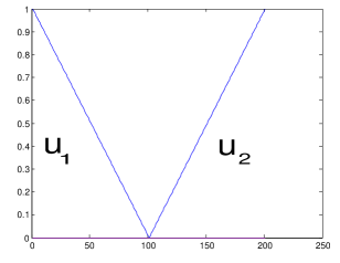
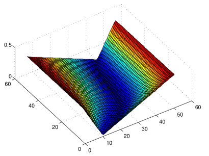
In Figure 1 we consider the set $\Omega=[-1,1],$ and $f_{1}$ and $f_{2}$ taken to be constant. The free boundaries are clearly visible. It is easy to see that the smaller dynamics $f_{i}$ provides $u_{i}$ more captured place.

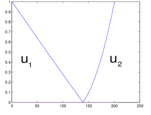
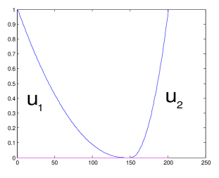
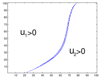
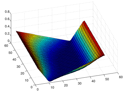
Next we present numerical examples in $2D.$ In Figures 2 and 3 we take $\Omega=[0,1]\times[0,1],$ with the boundaries $\phi_{1}(x,y)$ and $\phi_{2}(x,y)$ defined by:

$$\phi_{1}(x,0)=\left\{\begin{array}[]{ll}0.5-2.5x&0\leq x\leq 0.2,\\ 0&0.2\leq x\leq 1,\end{array}\right.\hskip 7.22743pt\phi_{1}(x,1)=\left\{\begin{array}[]{ll}0.5-\frac{5}{8}x&0\leq x\leq 0.2,\\ 0&0.8\leq x\leq 1,\\ \end{array}\right.$$

$$\phi_{1}(0,y)=0.5,\quad\quad\phi_{1}(1,y)=0,$$

and

$$\phi_{2}(x,0)=\left\{\begin{array}[]{ll}0&0\leq x\leq 0.2,\\ \frac{-1}{8}+\frac{5}{8}x&0.2\leq x\leq 1,\end{array}\right.\hskip 7.22743pt\phi_{2}(x,1)=\left\{\begin{array}[]{ll}0&0\leq x\leq 0.8,\\ -2+2.5x&0.8\leq x\leq 1,\\ \end{array}\right.$$

$$\phi_{2}(0,y)=0,\quad\quad\phi_{2}(1,y)=0.5,$$

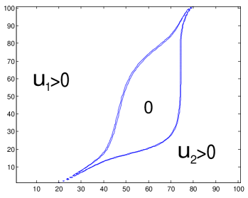
In Figure 2 we clearly see that the zero set does not appear and competing densities $u_{1}$ and $u_{2}$ meet each other along the whole free boundary, while in Figure 3 there is a zero set between the densities due to the big internal dynamics $f_{i}.$

(a) $f_{1}=f_{2}=0$

(b) $f_{1}=0$ and $f_{2}=3$

(c) $f_{1}=1$ and $f_{2}=8$

(d) $f_{1}=2$ and $f_{2}=8$

Figure 1. For all cases the boundaries are taken $\phi_{1}(-1)=\phi_{2}(1)=1$ and $\phi_{2}(-1)=\phi_{1}(1)=0.$

(a) $u_{1}+u_{2}$

(b) Free Boundaries

Figure 2. Internal dynamics are taken $f_{1}=0$ and $f_{2}=5.$

(a) $u_{1}+u_{2}$

(b) Free Boundaries

Figure 3. Internal dynamics are taken $f_{1}=4$ and $f_{2}=12.$

References

- [1] Arakelyan, A. A finite difference method for two-phase parabolic obstacle-like problem. Armenian Journal of Mathematics 7, 1 (2015), 32–49.
- [2] Arakelyan, A., Barkhudaryan, R., and Poghosyan, M. Numerical solution of the two-phase obstacle problem by finite difference method. submitted.
- [3] Arakelyan, A. G., Barkhudaryan, R. H., and Poghosyan, M. P. Finite difference scheme for two-phase obstacle problem. Dokl. Nats. Akad. Nauk Armen. 111, 3 (2011), 224–231.
- [4] Bozorgnia, F. Numerical algorithm for spatial segregation of competitive systems. SIAM J. Sci. Comput. 31, 5 (2009), 3946–3958.
- [5] Bozorgnia, F. Numerical solutions of a two-phase membrane problem. Applied Numerical Mathematics 61, 1 (2011), 92–107.
- [6] Bozorgnia, F., and Arakelyan, A. Numerical algorithms for a variational problem of the spatial segregation of reaction–diffusion systems. Applied Mathematics and Computation 219, 17 (2013), 8863–8875.
- [7] Conti, M., Terracini, S., and Verzini, G. Asymptotic estimates for the spatial segregation of competitive systems. Adv. Math. 195, 2 (2005), 524–560.
- [8] Conti, M., Terracini, S., and Verzini, G. A variational problem for the spatial segregation of reaction-diffusion systems. Indiana Univ. Math. J. 54, 3 (2005), 779–815.
- [9] Conti, M., Terracini, S., and Verzini, G. Uniqueness and least energy property for solutions to strongly competing systems. Interfaces Free Bound. 8, 4 (2006), 437–446.
- [10] Crooks, E. C. M., Dancer, E. N., and Hilhorst, D. Fast reaction limit and long time behavior for a competition-diffusion system with Dirichlet boundary conditions. Discrete Contin. Dyn. Syst. Ser. B 8, 1 (2007), 39–44 (electronic).
- [11] Crooks, E. C. M., Dancer, E. N., and Hilhorst, D. On long-time dynamics for competition-diffusion systems with inhomogeneous Dirichlet boundary conditions. Topol. Methods Nonlinear Anal. 30, 1 (2007), 1–36.
- [12] Crooks, E. C. M., Dancer, E. N., Hilhorst, D., Mimura, M., and Ninomiya, H. Spatial segregation limit of a competition-diffusion system with Dirichlet boundary conditions. Nonlinear Anal. Real World Appl. 5, 4 (2004), 645–665.
- [13] Dancer, E. N., and Du, Y. H. Competing species equations with diffusion, large interactions, and jumping nonlinearities. J. Differential Equations 114, 2 (1994), 434–475.
- [14] Dancer, E. N., Hilhorst, D., Mimura, M., and Peletier, L. A. Spatial segregation limit of a competition-diffusion system. European J. Appl. Math. 10, 2 (1999), 97–115.
- [15] Dancer, E. N., and Zhang, Z. Dynamics of Lotka-Volterra competition systems with large interaction. J. Differential Equations 182, 2 (2002), 470–489.
- [16] Petrosyan, A., Shahgholian, H., and Ural’ceva, N. N. Regularity of free boundaries in obstacle-type problems, vol. 136. American Mathematical Soc., 2012.
- [17] Squassina, M. On the long term spatial segregation for a competition-diffusion system. Asymptot. Anal. 57, 1-2 (2008), 83–103.
- [18] Squassina, M., and Zuccher, S. Numerical computations for the spatial segregation limit of some 2D competition-diffusion systems. Adv. Math. Sci. Appl. 18, 1 (2008), 83–104.
- [19] Weiss, G. S. Partial regularity for weak solutions of an elliptic free boundary problem. Comm. Partial Differential Equations 23, 3-4 (1998), 439–455.