The formation of IRIS diagnostics
II. The formation of the MG II H&K lines in the solar atmosphere

Abstract

NASA’s Interface Region Imaging Spectrograph (IRIS) small explorer mission will study how the solar atmosphere is energized. IRIS contains an imaging spectrograph that covers the Mg II  h&k lines as well as a slit-jaw imager centered at Mg II k. Understanding the observations requires forward modeling of Mg II  h&k line formation from 3D radiation-MHD models. This paper is the second in a series where we undertake this modeling. We compute the vertically emergent h&k intensity from a snapshot of a dynamic 3D radiation-MHD model of the solar atmosphere, and investigate which diagnostic information about the atmosphere is contained in the synthetic line profiles.

We find that the Doppler shift of the central line depression correlates strongly with the vertical velocity at optical depth unity, which is typically located less than 200 km below the transition region (TR). By combining the Doppler shifts of the h and the k line we can retrieve the sign of the velocity gradient just below the TR. The intensity in the central line depression is anticorrelated with the formation height, especially in subfields of a few square Mm. This intensity could thus be used to measure the spatial variation of the height of the transition region.

The intensity in the line-core emission peaks correlates with the temperature at its formation height, especially for strong emission peaks. The peaks can thus be exploited as a temperature diagnostic. The wavelength difference between the blue and red peaks provides a diagnostic of the velocity gradients in the upper chromosphere. The intensity ratio of the blue and red peaks correlates strongly with the average velocity in the upper chromosphere.

We conclude that the Mg II  h&k lines are excellent probes of the very upper chromosphere just below the transition region, a height regime that is impossible to probe with other spectral lines. They also provide decent temperature and velocity diagnostics of the middle chromosphere.

1. Introduction

This is the second paper in the series exploring the diagnostic potential of the Mg II  h&k lines in preparation for NASA’s Interface Region Imaging Spectrograph (IRIS) space mission. In paper I we discuss the feasibility of modeling these lines in non-LTE and with partial frequency redistribution (PRD) in increasingly realistic Radiation-Magneto Hydrodynamic (RMHD) simulations. We find that the h&k resonance lines can be modeled reliably with a 4-level plus continuum atomic model of Mg II, comprised of the $3s\,^{2}\!S$ ground state, the two $3p\,^{2}\!P$ levels, an artificial level representing higher energy levels to correctly reproduce the Mg II–Mg III ionization balance, and the Mg III ground state. The calculations presented in paper I also make clear that PRD always needs to be accounted for. For wavelengths in the line wings up to and including the k₂ and h₂ peaks, 1D column-by-column radiative transfer suffices to accurately reproduce profile shapes and their spatial variations. For line-core wavelengths between the emission peaks 3D transfer is required, but complete redistribution (CRD) is sufficient.

Because of its large abundance and the dominance of its singly ionized state the Mg II  h&k lines sample higher layers of the solar chromosphere than other common diagnostics of that region, namely H $\alpha$, the Ca II H&K lines, the Ca II IR triplet lines and the He I 1083 nm subordinate line.

The difference in formation height of several of these diagnostics as expressed by the maximum height where $\tau\!=\!1$ over the line profile at each location and calculated through a $yz$-slice from the 3D RMHD atmosphere employed in Paper I is plotted in Figure 1. The CaII K, Ca II 854.2 nm (as representative of the IR triplet) and H $\alpha$ formation heights (see Leenaarts et al., 2012) were computed in 3D non-LTE using Multi3d. Clearly Mg II k and Ca II K have very similar formation properties, with the main difference between them the higher opacity due to the larger solar abundance of magnesium (7.60 for Mg and 6.34 for Ca, Asplund et al., 2009), which, all else equal, translates to a difference in $\tau\!=\!1$ height of 2.9 scale heights. The larger magnesium opacity leads also to a larger thermalization depth and thus magnesium retains temperature sensitivity in the source function to larger heights. This sensitivity is reflected in the fact that Mg II k shows central reversals in the line core everywhere (Morrill et al., 2001) while Rezaei et al. (2008) report that 25% of the internetwork Ca II H profiles show a reversal-free line core.

Observations in all lines mentioned above show elongated fibrilar structure that most likely are to a large extent aligned with the magnetic field. All lines can thus be used to study morphology. Yet, observations in one single line alone cannot yield a sufficiently complete picture of physical processes in the chromosphere due to the limits in formation height range and the usability of each line to infer all relevant physical parameters: mass density, temperature, velocity and magnetic field.

So far, multi-wavelength studies of the chromosphere have mainly utilized H $\alpha$ and Ca II 854.2 nm (e.g.,, Cauzzi et al., 2009; Sekse et al., 2012; Reardon et al., 2009), which in our model atmosphere form roughly at equal height, approximately the same height as optical depth unity for the Mg II  h&k emission peaks (see Figure 6).

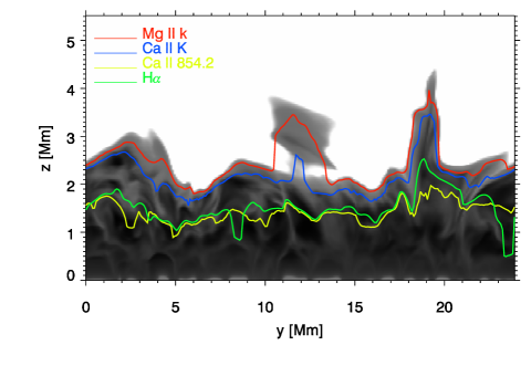
Figure 1.— Differences between $\tau\!=\!1$ heights of Mg II k, Ca II K, Ca II 854.2 nm and H $\alpha$ in an $yz$-slice of the 3D model atmosphere. The image displays the temperature, clipped at 20 kK, with curves of the maximum $\tau\!=\!1$ height of the various lines overplotted.

The two lines are, however, used very differently. The H $\alpha$ line core intensity and width are density and temperature diagnostics (Leenaarts et al., 2012), while the Ca II 854.2 nm line can be used as velocity and temperature diagnostic, and, if observing the full Stokes vector at sufficient sensitivity, magnetic field strength and orientation (de la Cruz Rodríguez et al., 2012). Since, in the weak field limit (Stenflo, 1994, p. 258), the amount of circular polarization due to the Zeeman effect in a spectral line is proportional to the ratio of the line splitting over the Doppler width, and the amount of linear polarization proportional to the square of that ratio, we can expect only very weak polarization signals in any of the other chromospheric lines because the h&k and H&K lines are too far to the blue and H$\alpha$ has a Doppler width that is too large (Uitenbroek, 2011). The only other truly chromospheric spectral line that can be used effectively for magnetometry is the He I 1083 nm line, which can be used to measure strength and orientation of weak and strong magnetic fields because of its sensitivity to both the Zeeman and Hanle effects (Asensio Ramos et al., 2008).

Through its capability of obtaining spectra of the Mg II  h&k lines at high spatial, spectral and temporal resolution the IRIS mission will provide a unique opportunity to extend multi-layer studies of the solar chromosphere to the region just below the transition region, which cannot be probed by other means. In this paper we focus on determining what diagnostic information can be obtained from observation of Mg II  h&k spectra by forward modeling of these lines through the same snapshot of a 3D RMHD simulation used in Leenaarts et al. (2012) and in paper I. Among other findings we show that the magnesium resonance lines provide excellent velocity diagnostics through the Doppler shift of h₃ and k₃ and an indication of the spatial variation of the height of the transition region through the intensity of h₃ and k₃.

The structure of the paper is as follows: In Section 2–3 we describe our 3D model atmosphere and the radiative transfer computations. Section 4 describes the reduction of the synthetic data to the intensity and Doppler-shift of the central emission peaks (k₂ and h₂) and the central minima (k₃ and h₃), the parameters that we use to characterize the line profiles. In Section 5–6 we describe how these parameters correlate with properties of the model atmosphere. In Section 7 we describe the formation of three example profiles in detail to illustrate the correlations that we found. We finish with a discussion of the results and our conclusions in Section 9.

2. Model atmosphere

We study the h&k line formation in a snapshot of a 3D radiation-MHD simulation performed with the Bifrost code (Gudiksen et al., 2011). The same snapshot has been used by Leenaarts et al. (2012) to investigate H $\alpha$ line formation and was also used in Paper I. A 2D slice through this atmosphere was used by Štěpán et al. (2012) to investigate depolarization of scattered light by the Hanle effect in the Lyman-$\alpha$ line.

Bifrost solves the equations of resistive MHD on a staggered Cartesian grid with a selection of modules describing various physical processes. The simulation we use here included radiative transfer in four multi-group opacity bins including coherent scattering affecting the energy balance in the photosphere and low chromosphere (Nordlund, 1982; Skartlien, 2000; Hayek et al., 2010) parametrized radiative losses in the upper chromosphere, transition region and corona (Carlsson & Leenaarts, 2012), thermal conduction along magnetic field lines (Gudiksen et al., 2011) and an equation of state that includes the effects of non-equilibrium ionization of hydrogen (Leenaarts et al., 2007).

The simulation covers a physical extent of $24\times 24\times 16.8$ Mm³, with a grid of $504\times 504\times 496$ cells, extending from 2.4 Mm below the average height of $\tau_{500}=1$ to 14.4 Mm above covering the upper convection zone, photosphere, chromosphere and the lower corona. The horizontal axes have an equidistant grid spacing of 48 km, the vertical grid spacing is non-uniform, with a spacing of 19 km between $z=-1$ and $z=5$ Mm. The spacing increases towards the bottom and top of the computational domain to a maximum of 98 km. The simulation contains a magnetic field with a an average unsigned strength of 50 G in the photosphere, concentrated in the photosphere in two clusters of opposite polarity 8 Mm apart. For further details on this snapshot we refer to Leenaarts et al. (2012).

3. Radiative transfer computations

We perform non-LTE radiative transfer computations using the 4-level-plus-continuum model atom from paper I with two different codes: The first is a version of RH by Uitenbroek (2001), modified to use MPI so it can efficiently solve the radiative transfer in all columns in the 3D model atmosphere assuming each column is a plane-parallel 1D atmosphere, including angle-dependent partial redistribution.

The second code we use is Multi3d (Leenaarts & Carlsson, 2009). This is an MPI-parallelized radiative transfer code that can evaluate the radiation field in full 3D, taking the horizontal structure in the model atmosphere into account. For this 3D computation we reduced the grid size of the model atmosphere to $252\times 252\times 200$ grid cells to reduce the amount of computational work.

The Mg II  h&k lines are influenced by both PRD and 3D effects. We lack the capability to compute both simultaneously, so for the analysis of the line profiles we use the hybrid approach described and motivated in Paper I: we use 1D PRD computations with RH for the line profile up to and including the central emission peaks. The intensity of the central line depression is taken from the 3D CRD computation with Multi3d.

4. Reduction of the synthetic spectra

4.1. Line parameters

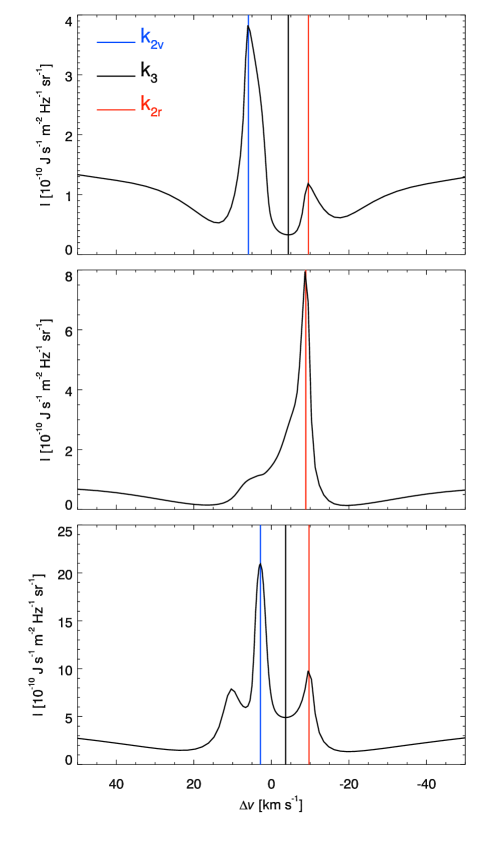
Figure 2.— Example Mg II k line profiles with the identification of the k_2V, k₃ and k_2R features. Top: standard profile with two emission peaks and a central depression. Middle: profile showing only one emission peak on the red side of the rest line-center wavelength. Bottom: profile showing three emission peaks. The vertical blue, black and red lines indicate the wavelength position of k_2V, k₃ and k_2R as determined by our algorithm.

Each of the Mg II  h&k lines, as seen in solar observations, is often characterized by a central absorption core surrounded by two emission peaks that are in turn surrounded by local minima. These features are often refered to as h₃ and k₃ (line cores), h₂ and k₂ (peaks), and h₁ and k₁ (outer minima of peaks). The red and blue sides of the peaks and minima are distinguished with the added subscript of R or V respectively. This simplistic description is at odds with many of the spatially-resolved spectra of our calculations as the synthetic line profiles can show a more complex structure. We find line profiles that have from zero to as many as six emission peaks. Nevertheless, the majority of line profiles shows a more conventional profile with two outer minima, two emission peaks and a central minimum. Out of the 254 016 columns of our 1D computation, 0.1% of the profiles did not have any emission peaks, 1.6% had one peak, 66.6% had two peaks and 31.7% had three or more peaks.

To understand how the spectral properties relate to the physical properties of the atmosphere, we extracted the positions of the line cores and red and blue peaks from the spectra. For each of these features we extracted the intensity and spectral position (here measured in Doppler shift relative to the rest wavelength of the line center, for brevity referred to as ‘velocity shift’). Throughout the paper we use the convention that a positive Doppler shift corresponds to a blueshift, and a positive velocity in the model atmosphere corresponds to an upflow.

Given the large variation of the profile shapes, in some cases some of these features will not be present, or are difficult to identify. Also, given the large number of spectra, we needed to use an automated procedure to extract the quantities. Both the automated detection and the exotic line profiles introduce uncertainties in our analysis, of which the reader should be aware.

In the top panel of Figure 2 we show a ‘standard’ profile, with well-defined features. The middle panel shows a profile with only one emission peak, labeled as k_2R because it has a wavelength larger than the rest line center wavelength. In this case the k_2V and k₃ features are not defined. The bottom panel shows a triple-peaked profile. For profiles with three or more peaks it is not a priori clear which features to select. We detail the assumptions we used in our extraction algorithm below.

4.2. Extraction algorithm

To extract the positions of the line core and peaks we start by using an extremum-finding algorithm on a small spectral region ($-40<\Delta v<40$ km s^-1) around the rest wavelength of each line. This gives us the wavelengths of all maxima and minima in each line-core spectrum.

Then we extract the line center position. Depending on the number of maxima and minima found, we employed a few rules to obtain an initial estimate of the line center velocity shift. Most of the profiles have an odd number of minima (usually two maxima and one minimum) – for these we use the middle minimum. If there are an even number of minima we use the one with the lowest intensity. If no minima are found, we use a default value of $\Delta v$=5 km s^-1. Using the estimate for the line center velocity, a parabolic fit is made to a few spectral points around the estimate. This yields the line center velocity and intensity. If these results are too far from the starting estimate (i.e.,, an erroneous fit), the spectrum will be marked as outlier (see below). To improve the accuracy and purge spurious results, we try to enforce a smooth spatial distribution of the line centre shifts. Using a spatial convolution we identify pixels with a significant difference to the neighboring values. For these ‘outliers’ we redo the line center fit, using as starting estimate a weighted mean of the surrounding pixels.

The next part of the procedure is to extract the coordinates of the red and blue peaks. As for the line center, we use the number of maxima and minima to estimate the peak locations. Maxima whose absolute distance to the line center is larger than 30 km s^-1 are discarded. If there are more than four maxima, only the inner four are used. Whether maxima are assigned as estimates of the red or blue peaks will depend on their position relative to the line core (red-ward or blue-ward). If the profile has two maxima these are used as estimates for the red and blue peaks. If there are three maxima, we take the closest to the line centre and the strongest of the remaining. If there are four maxima, we use the inner maxima unless they are very close together and have low intensities (i.e.,, spurious peaks). Using the estimates for the peaks, the spectra are interpolated with a cubic spline on a high resolution wavelength grid. The velocity shifts and intensities for the peaks are obtained from the interpolated spectral maxima.

We thoroughly tested the algorithm and in the overwhelming majority of the cases it found the same spectral features as what a manual visual inspection would produce. As mentioned before, in certain pixels some of the spectral features are absent and are marked as such.

4.3. Overview of results

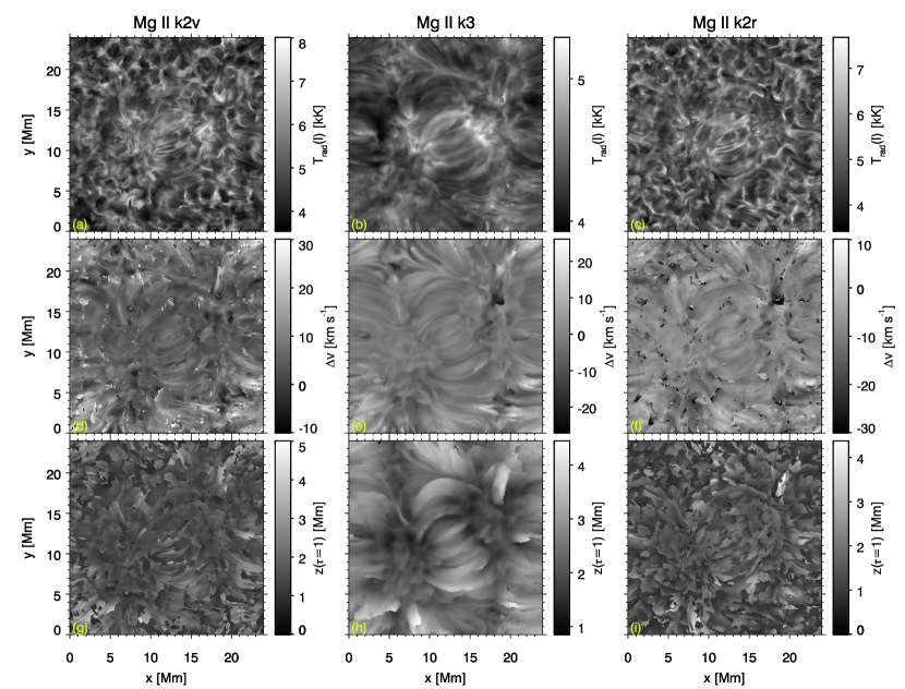
Figure 3.— Intensity (top row), Doppler shift (middle row, positive is blueshift) and height of optical depth unity (bottom row) in the k_2V (left column), k₃ (middle column) and k_2R (right column) features. Absent features and misidentifications show up as small white and black spots and patches, especially visible in panels (d) and (f).

Figure 3 shows images for the intensity and Doppler shift relative to the line-center rest frequency of the features in the k line, together with the height of optical depth unity at the feature. The k_2V and k_2R intensity (panels (a) and (c)) show a pattern reminiscent of chromospheric shocks around the edges of the image, with a weak imprint of elongated, magnetically formed structures in the image center. In contrast, the k₃ image (panel (b)) shows elongated structures that are aligned with the chromospheric magnetic field structure in the whole image.

The second row shows the Doppler shift. Interestingly, the k_2V and k_2R panels (d) and (f) show elongated large-scale structure, with many similarities to the k₃ Doppler shift (panel (e)). In Sections 5–6 we show that the Doppler shift of k_2V, k_2R and k₃ are all determined by the velocity in the upper chromosphere, and thus show a correlation.

The bottom row of Figure 3 shows the height of optical depth unity. Panels (g) and (i) show that the $\tau\!=\!1$ height displays an irregular leaf-like structure for k_2V and k_2R. Panel (h) displays a much smoother structure, again aligned with the magnetic field lines.

4.4. On displaying correlations

In Figures 4–8 we show correlations between synthetic observables and properties of the model atmosphere. Due to the large number of pixels in our snapshot (63,504 for the 3D computation and 254,016 in the 1D computation), a scatter plot where each pixel is represented with a black dot would lead to a completely saturated image.

Another option is to compute the numerical approximation of the joint probability density function (JPDF). This approach has the advantage that saturation does not occur, but the drawback is that the part of parameter space with a low density is hard to see.

A third option is to compute the JPDF, and then scale each column or row to maximum contrast, so that each column is a one-dimensional histogram. This way correlations also show where the JPDF has low density, but the shape of the original JPDF is lost.

No solution is ideal, so as a compromise we plot the JPDF with each column scaled to maximum contrast in order to identify correlations throughout the parameter space, and overplot contours of constant density in the original JPDF containing 50% and 90% of all points to provide an indication of the shape of the JPDF.

5. Diagnostic information in h3 and k3

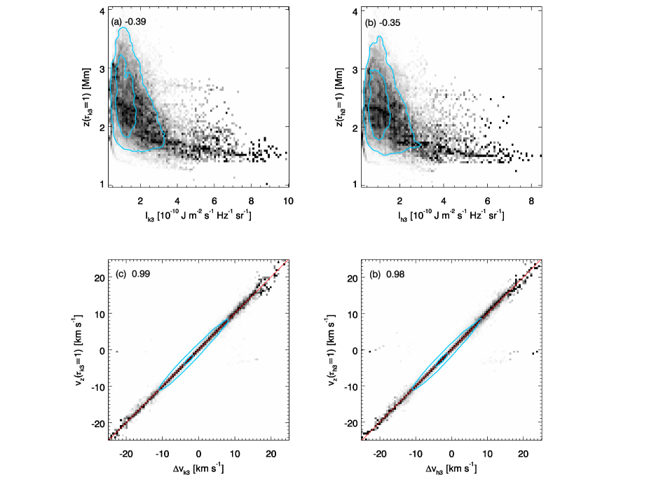
Figure 4.— Scaled joint probability density functions (JPDF) of $\tau\!=\!1$ height versus the intensity (panels a and b) and vertical velocity at the $\tau\!=\!1$ height versus the Doppler shift (panels c and d) of the k₃ and h₃ line centers. The inner blue contour includes 50% of all pixels, the outer contour 90%. Each column in the panels is scaled to maximum contrast to increase visibility. The Pearson correlation coefficient is given in the upper left corner next to the panel label. Left column is for the k line, right column for the h line. (a)-(b) $\tau\!=\!1$ height of line center versus line center intensity; (c)-(d) vertical velocity at the $\tau\!=\!1$ height of line center (positive is upflow) versus the Doppler shift of line center (positive is blueshift), the red line denotes the line $y=x$.

In this section we investigate the diagnostic potential of k₃ and h₃ from their observed quantities: intensities and Doppler shifts. We searched for correlations between these quantities and the properties of the atmosphere.

5.1. Line core velocities

The Doppler shift relative to the rest-frame line center wavelength contains information on the line-of-sight velocity in the atmosphere. In panels (c) and (d) of Figure 4 we show the correlation between the Doppler shift and the vertical velocity at optical depth unity. The correlation is tight, the correlation coefficient is very close to unity, the FWHM of the $v_{z}(\tau\!=\!1)$ velocity distribution at fixed Doppler shift is typically 0.5 km s^-1. This makes k₃ and h₃ excellent velocity diagnostics.

Furthermore, the small difference between the k₃ height of optical depth unity and the height of the transition region in our model suggests that these spectral features can be used to measure the velocity in the very upper chromosphere. This is impossible to do with chromospheric lines observed from the ground as H $\alpha$, Ca II 854.2 nm and Ca II H&K, as these lines have a lower opacity and therefore form further below the transition region (see Section 1).

5.2. Line core intensities

Panels (b) and (h) of Figure 3 suggest some anti-correlation between the intensity and formation height. We confirm this in panels (a) and (b) of Figure 4, which show the JPDF of the intensity and the height of optical depth unity of k₃ and h₃. At locations where the intensity is low, the height of optical depth unity tends to be large. The correlation is weak and the JPDF displays a large spread. The reason for this anti-correlation is the 3D scattering of the radiation in the chromosphere.

The cores of Mg II  h&k form in a low density environment with a large photon mean free path and low photon destruction probability. As a consequence the local radiation field is smoothed horizontally and, on average, decreases with height. The Eddington-Barbier relation is valid, and the emergent intensity is thus approximately equal to the source function at optical depth unity. The latter is equal to the angle-averaged radiation field. The source function is low at large $\tau\!=\!1$ heights, and therefore the emergent intensity is low too. The same mechanism acts in the H $\alpha$ line core, as explained by Leenaarts et al. (2012). The Mg II  h&k anticorrelation of formation height and intensity is weaker than for H $\alpha$ mainly for two reasons. First, the h&k lines are resonance lines and lack the mid-chromospheric opacity gap of H $\alpha$; they thus have less smoothing of the radiation field. Second, the h&k Doppler width is smaller than for H $\alpha$ and the source function at the wavelengths of k₃ and h₃ is therefore more sensitive to the velocity field.

We computed the Pearson correlation coefficient for smaller 2 Mm $\times$ 2 Mm subfields and found much tighter correlation, with correlation coefficients typically between -0.9 and -0.6. This indicates that at such scales the radiation field is smooth enough to use the intensity as a relative height measurement.

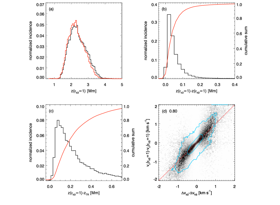
Figure 5.— Formation properties of k₃ and h₃. (a) Histogram of the height of optical depth unity of k₃ (black) and h₃ (red). (b) Histogram of difference of the heights of optical depth unity of k₃ and h₃ (black, left-hand scale). The cumulative sum of the histogram is shown with the red curve and the right-hand scale. (c) Histogram of difference of the height of the transition region in the 3D model and the height of optical depth unity of k₃ (black, left-hand scale). The cumulative sum of the histogram is shown with the red curve and the right-hand scale; (d) Scaled joint probability density function of the difference of the velocity at optical depth unity of k₃ and h₃ versus the difference in Doppler shift of k₃ and h₃. The inner blue contour includes 50% of all pixels, the outer contour 90%. Each column in the panels is scaled to maximum contrast to increase visibility. The Pearson correlation coefficient is given in the upper left corner. The red line denotes the line $y=x$.

5.3. Combining k₃ and h₃

By combining the h and k lines one can extract additional information, namely the difference in velocity in the atmosphere between the slightly different heights of optical depth unity. In panel (a) of Figure 5 we show the histograms of the $\tau\!=\!1$ height of k₃ and h₃. The k₃ distribution is shifted to slightly larger heights. In panel (b) this is shown in more detail, where we plot the histogram of the difference in height of optical depth unity between k₃ and h₃. The k₃ minimum typically forms a few tens of kilometers higher.

In panel (c) we show where in the chromosphere optical depth unity of k₃ is reached. It shows the histogram of the height difference between the transition region and $z(\tau_{\mathrm{k3}}\!=\!1)$. We define the height of the transition region in a column in the atmosphere as the largest height where the temperature drops below 30 kK. The k₃ minimum forms typically less than 200 km below the transition region. Finally, in panel (d) we show the JPDF of the difference in observed Doppler shift of the h and k minima $\Delta v_{\mathrm{k3}}-\Delta v_{\mathrm{h3}}$ and the difference in velocity at optical depth unity $v(\tau_{\mathrm{k3}}\!=\!1)-v(\tau_{\mathrm{h3}}\!=\!1)$. There is a clear correlation between the two, with a correlation coefficient of 0.80. The correlation is good enough to detect the sign and possibly the magnitude of the velocity difference. This opens up the possibility to detect short-wavelength velocity oscillations and measure the vertical acceleration of upper-chromospheric material with an instrument with sufficiently high spatial and spectral resolution.

6. Diagnostic information of h2 and k2

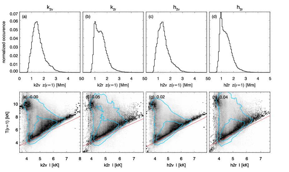
Figure 6.— Formation properties of the Mg II  h&k line-core emission peaks Top row (panels (a)–(d)): histogram of the height of optical depth unity for the spectral feature indicated above the panels. Bottom row (panels (e)–(h)): Scaled joint probability density functions the temperature at the height of optical depth unity versus the intensity of the emission peaks expressed as a radiation temperature. The inner blue contour includes 50% of all pixels, the outer contour 90%. Each column in the panels is scaled to maximum contrast to increase visibility. The red lines denote the line $y=x$. The Pearson correlation coefficient is given in the upper left corner of each panel.

We now turn our attention to the diagnostic information contained in the intensities and Doppler shifts of the k_2V, k_2R, h_2V and h_2R peaks.

6.1. Peak intensities

In Figure 6 we show histograms of the $\tau\!=\!1$ heights for the k_2V, k_2R, h_2V and h_2R peaks, and JPDFs of the peak intensity and the temperature at their $\tau\!=\!1$ height. The distribution of $\tau\!=\!1$ heights peaks between 1 and 2 Mm, with a tail up to beyond 3 Mm. This tail is caused by the large variations of the opacity from velocity variations along the line-of-sight. The contribution function at the wavelength of the intensity peaks can therefore be bimodal, with a contribution from the middle chromosphere and a contribution from higher up in the chromosphere. The $\tau\!=\!1$ height can be in either location (see also Section 7 and Figure 11). The median height of optical depth unity is highest for k_2V (1.46 Mm), and lowest for h_2R (1.29 Mm). The blue peaks form on average 60 km higher than the red peaks.

Panels (e)–(f) show JPDFs of $T(\tau\!=\!1)$ versus the intensity. The distributions have a typical structure. For many of the points there is a very good correlation between intensity and temperature. For these points the gas temperature is about 500 K larger than the radiation temperature. These are the columns whose $\tau\!=\!1$ heights are located in the mid-chromosphere, around 1.5 Mm. Here the source function is only partially decoupled from the local temperature, causing the correlation. This correlation is more tightly constrained for larger intensities. At lower intensities the distribution widens, with a fraction of the pixels having a gas temperature higher than the radiation temperature. In these columns the $\tau\!=\!1$ heights are located mostly in the upper chromosphere, where the source function is completely decoupled from the temperature. Note that the intensity-temperature correlation is stronger for the blue peaks than for the red peaks.

The correlation shows that large peak intensities are a good diagnostic of the temperature at the heigth of optical depth unity. The same holds for a fraction of the pixels with lower peak intensities, but at low peak intensities there is also a fraction for which it is not.

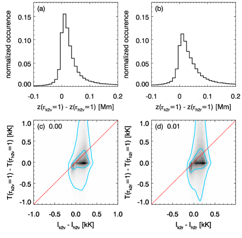
Figure 7.— Formation height differences between the emission peaks and the correlation between peak intensity and temperature at optical depth unity. (a) histogram of the difference of $\tau\!=\!1$ height of k_2V and h_2V; (b) same as (a) but for the red peaks; (c) Joint probability density function of the difference of the temperature at the $\tau\!=\!1$ height of k_2V and h_2V versus the difference of the intensity of k_2Vand h_2V. The inner blue contour includes 50% of all pixels, the outer contour 90%. The red line denotes $y=x$. The Pearson correlation coefficient is given in the upper left corner of the panel; (d) same as (c) but for the red peaks.

We also investigated whether it is possible to measure the sign of the temperature gradient by exploiting the slight difference in $\tau\!=\!1$ heights between the h and the k line. We show the results in Figure 7. Panel (a) shows a histogram of the difference in $\tau\!=\!1$ heights between k_2V and h_2V. Panel (b) shows the same for the red peaks. In the majority of cases the peaks of the k line form between 0 and 100 km higher. Panel (c) shows the JPDF of the intensity difference between k_2V and h_2V, and the difference in temperature at the height of optical depth unity. There is no usable correlation. The same holds for the red peaks, as shown in panel (d). The scattering contribution to the source function adds so much variation that the temperature differences between the formation heights are washed out in the emergent intensity.

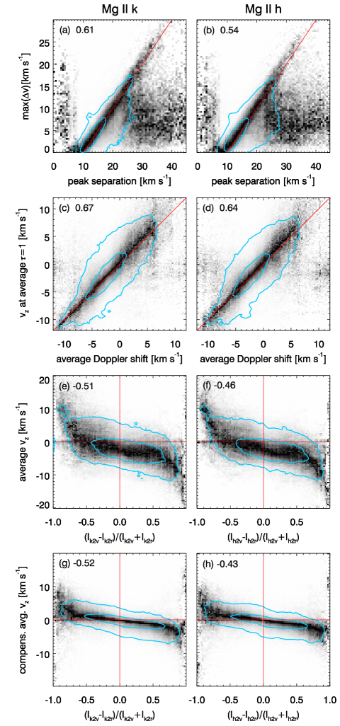
Figure 8.— Velocity information contained in k₂ (left column) and h₂(right column). The correlations are shown as scaled JPDFs. The inner blue contour includes 50% of all pixels, the outer contour 90%. Each column in the panels is scaled to maximum contrast to increase visibility. The Pearson correlation coefficient is given in the upper left corner of each panel. (a)-(b) velocity difference between the blue and red peaks vs. $\max(\Delta v)$ (see text), the red line is $y=x-10$; (c)-(d) Mean Doppler shift of the blue and red peak vs. the vertical velocity at the mean $\tau\!=\!1$ height of the peaks; (e)-(h) normalized difference of the peak intensities vs. the mean vertical velocity in the atmosphere between the mean $\tau\!=\!1$ height of the emission peaks and the line core, the red lines denote $x=0$ and $y=0$; (g)-(h) same as (e)-(h), but now for the compensated mean vertical velocity (see text).

6.2. Peak velocities

The k₂ and h₂ peaks form deeper than the line cores, and thus provide velocity diagnostics for a different height in the chromosphere. To investigate what information about the atmospheric velocity is contained in the peaks, we investigated the following observable quantities: peak separation, average Doppler shifts, and peak intensity ratios. Figure 8 shows the results.

The peak separation is a measure of the width of the extinction profile, and is sensitive to the velocity variations in the upper chromosphere. At typical chromospheric temperatures the thermal width of the extinction profile is relatively small, on the order of 2.5 km s^-1. In an atmosphere without velocity fields this leads to a small peak separation. Velocity gradients in the atmosphere work to widen the peak separation, by causing height-dependent wavelength shifts of the narrow thermal extinction profile. The height-integrated extinction coefficient will then be wider than the extinction profile at any given fixed height.

For each pixel in the synthetic spectra we measured the peak separation between the blue and red peaks in each line. Then we computed $\max(\Delta v)$, the difference between the maximum and minimum atmospheric velocities in the formation region of the inter-peak profile (defined as the range between the average $\tau\!=\!1$ height of the emission peaks and the $\tau\!=\!1$ height of the line core minimum). Panels (a)-(b) show the JPDF of the peak separation and the maximum velocity difference. There is a clear positive correlation between the two quantities: a larger peak separation corresponds to a larger velocity difference in the chromosphere above the formation height of the peaks.

A small quantity of points (less than 10%) does not follow the near-linear relation between peak separation and $\max(\Delta v)$. They have a large peak separation and small $\max(\Delta v)$. These points have two origins. Some points result from a misidentification from our algorithm. This typically happens when one of the peaks is almost non-existent and a smaller spectral feature is mistakenly assumed to be the peak, or when there are multiple clear peaks and our algorithm selects the wrong peak. For the points that have $\max(\Delta v)$ less than the peak separation minus 15 km s^-1, about half of them result from these misidentifications. The other half is caused by a naturally wider extinction profile that happens when there is a temperature maximum in the lower chromosphere ($z\approx 0.6-0.9$ Mm). In these cases the source function has a maximum at heights lower than usual. This results in a larger peak separation due to the atmospheric temperature structure instead of velocities.

We expect the velocity around the formation heights of the peaks to influence the wavelength location of the peaks. To investigate this we computed the average Doppler shift of the k_2V and k_2R peaks ($\Delta v_{\mathrm{Dop,k}}$) as follows:

$$\Delta v_{\mathrm{Dop,k}}=-\frac{1}{2}\frac{c}{\lambda_{\mathrm{k}}}\left[(\lambda_{\mathrm{k2v}}-\lambda_{\mathrm{k}})+(\lambda_{\mathrm{k2r}}-\lambda_{\mathrm{k}})\right],$$ (1)

with $c$, $\lambda_{\mathrm{k}}$, $\lambda_{\mathrm{k2v}}$ and $\lambda_{\mathrm{k2r}}$ respectively the speed of light, the rest-frame line center wavelength, the observed wavelength of k_2V and the observed wavelength of k_2R. With this definition a positive average Doppler shift corresponds to a blue shift. We then computed the atmospheric velocity at the average $\tau\!=\!1$ height of the peaks. The atmospheric velocity is defined such that upflows are positive. In panel (c) of Figure 8 we show the JPDF of these two quantities. There is a clear correlation between the atmospheric velocity and the Doppler shift, but the distribution shows some spread. Panel (d) shows the same for Mg II h.

From Carlsson & Stein (1997) we know that the Ca II H_2v and K_2v bright grains are strongest when the atmosphere above the formation height of the H_2v and K_2v peaks is moving down. The Mg II  h&k lines behave similarly, but exhibit stronger emission peaks because of their shorter wavelength and higher opacity. As line formation is almost symmetrical with respect to the line center wavelength, we expect that an upflow above the emission-peak formation height will lead to red peaks being stronger than blue peaks. The ratio of the blue and red peak intensity might thus be exploited to measure the average velocity in the upper chromosphere. It turns out that this is indeed the case. We computed the intensity ratio of the blue and the red peak as

$$R_{\mathrm{k}}=\frac{I_{\mathrm{k2v}}-I_{\mathrm{k2r}}}{I_{\mathrm{k2v}}+I_{\mathrm{k2r}}},$$ (2)

so that $I_{\mathrm{k2v}}>I_{\mathrm{k2r}}$ yields a positive peak ratio. We also computed the average vertical velocity in the atmosphere between the average $\tau\!=\!1$ height of the peaks and the $\tau\!=\!1$ height of k₃, i.e.,

$$v_{\mathrm{avg,k}}=\frac{\int_{z1}^{z2}v_{z}(z^{\prime})\mathrm{d}z^{\prime}}{z_{2}-z_{1}},$$ (3)

with

$$z_{1}=\frac{z(\tau_{\mathrm{k2v}}\!=\!1)+z(\tau_{\mathrm{k2r}}\!=\!1)}{2}$$ (4)

and

$$z_{2}=z(\tau_{\mathrm{k3}}\!=\!1).$$ (5)

As before, a positive velocity corresponds to upflow. The same procedure was followed for the h line. Panels (e)-(f) of Figure 8 show the JPDF of $R_{\mathrm{k/h}}$ and $v_{\mathrm{avg,k/h}}$. There is a correlation. A stronger blue peak corresponds to downflowing material above the peak formation height, and likewise, a stronger red peak corresponds to upflow. This is especially clear for large intensity ratios ($R>0.7$ and $R<-0.7$). For smaller ratios the correlation is weaker. Note that the majority of the distribution is below the zero line, indicating that there is on average a downward motion. This is partly due to a global oscillation in the simulation box (which at the time of this snapshot is directed downwards) and partly due to a correlation between density and velocity: upward moving waves have higher density in the upward phase than in the downward phase such that zero average mass-flow gives an average downward velocity.

The spread of the peak-intensity ratio versus velocity correlation can be significantly reduced by compensating for the velocity at the peak formation height. This is to be expected, because adding a constant velocity to the whole atmosphere would shift the line, but not change the intensity ratio. In panels (g)-(h) we show the peak ratio–velocity correlation again, but now we subtract the velocity at the average $\tau\!=\!1$ height of the peaks from $v_{\mathrm{avg,k/h}}$. This has two effects: one, the distribution is shifted upward and passes through the origin; two, the distribution at a given peak ratio is much narrower.

6.3. Summary

We summarize our analysis of the intensity and Doppler shift of the emission peaks:

• The emission peaks have optical depth unity at around $z\!=\!1.4$ Mm, but with a wide spread. The blue peaks form higher on average than the red peaks, and the k peaks higher than the h peaks. A fraction of the points has optical depth unity at larger heights (in the upper chromosphere).

• The peak intensity correlates very well with the gas temperature at optical depth unity, for peak radiation temperatures higher than 6 kK. At lower radiation temperatures this correlation has a larger spread, because more points reach an optical depth unity in the upper chromosphere, where the source function is completely decoupled from the local temperature.

• One cannot exploit the difference in optical depth unity between the h and k lines to measure the temperature gradient between these heights. The variation in intensity caused by the scattering part of the source function is larger than the sensitivity to temperature.

• The peak separation correlates well with the difference between maximum and minimum velocity in the chromosphere above above the height where the intensity peaks are formed. The average Doppler shift of the blue and red peaks exhibits a linear correlation with velocity at the average peak formation height.

• The peak intensity ratio can be used to constrain the average atmospheric velocity above the peak formation height: large peak intensity ratios indicate large flow velocities. Modest intensity ratios correlate with the difference in velocity at the peak formation height and the average velocity in the chromosphere above it.

We stress that all correlations have some spread.

7. Analysis of individual profiles

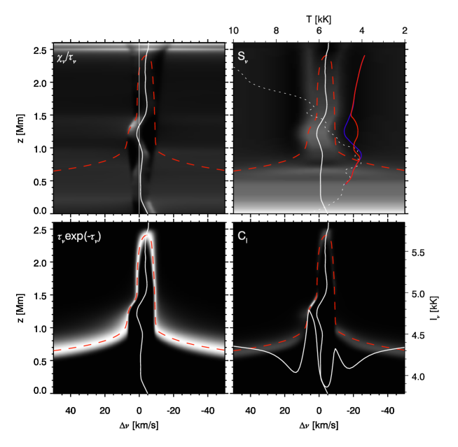
Figure 9.— Intensity formation breakdown figure for the Mg II k line. Each grey-scale image shows the quantity specified in its top-left corner as function of frequency from line center (in Doppler shift units) and simulation height $z$. Multiplication of the first three produces the intensity contribution function in the fourth panel. A $\tau_{\nu}\!=\!1$ curve (red dashed) and the vertical velocity (white solid, positive is upflow) are overplotted in each panel, with a $v_{z}\!=\!0$ line in the first panel for reference. The upper-right panel also contains the Planck function (dotted) and the line source function along the $\tau\!=\!1$ curve in blue for the part of the $\tau$ curve blueward of its maximum value and red for the part on the red side of the maximum $\tau\!=\!1$ height, in temperature units specified along the top. The lower-right panel also contains the emergent intensity profile, as brightness temperature with the scale along the right-hand side. The height scale is cut off where $T=30$ kK, i.e., in the transition region.

Figure 10.— Intensity formation breakdown figure for the Mg II k line. The description of the format is given in the caption of Fig. 9

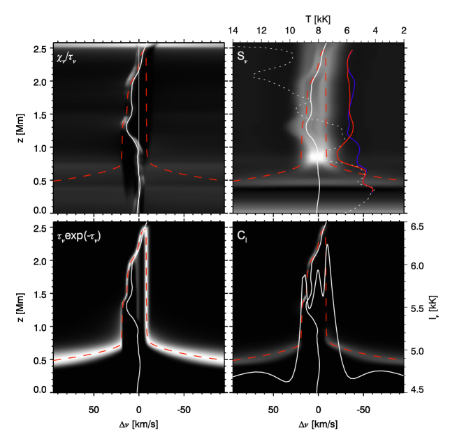
Figure 11.— Intensity formation breakdown figure for the Mg II k line. The description of the format is given in the caption of Fig. 9

So far we have studied the properties of the emergent Mg II  h&k line cores in a statistical manner. In this section we analyze the formation of the emergent line profile at three different locations in our 3D atmosphere, and discuss the physical mechanisms behind the correlations found in Sections 5 and 6. These profiles were computed in 1D with RH.

In Figures 9–11 we analyze the formation of the three different Mg II k profiles in detail using 4-panel formation diagrams introduced by Carlsson & Stein (1994, 1997). In these diagrams the contribution function $C_{I}$ to the vertically emergent intensity $I_{\nu}$ is shown as the product of three terms:

$$C_{I}=\frac{{\rm d}I_{\nu}}{{\rm d}z}=\frac{\chi_{\nu}}{\tau_{\nu}}\cdot S_{\nu}\cdot\tau_{\nu}\,{\rm e}^{-\tau_{\nu}},$$ (6)

with $z$, $\chi_{\nu}$, $\tau_{\nu}$ and $S_{\nu}$ the height in the atmosphere, the total extinction coefficient, the optical depth and the total source function. The latter three are frequency-dependent, indicated with the $\nu$ subscript. This decompositions shows that the contribution function to intensity peaks at locations of high opacity at low optical depth, around optical depth unity and with a high source function. The figures show these three terms and their product $C_{I}$. The large formation height range of the h&k lines, the small thermal line width and the frequency-dependent source function lead to complex formation behavior. To show the frequency-dependent source function behavior we add two curves to the source function panel. They show the source function along the $\tau\!=\!1$ curve in blue for the part of the $\tau$ curve blue ward of its maximum value and red for the part on the red side of the maximum $\tau\!=\!1$ height.

We start with discussing a rather standard line profile, with two clear emission peaks, the blue peak higher than the red peak, and a well defined central depression in Figure 9. This column in the atmosphere has a rather weak velocity field, with a slight upflow at 1.25 Mm and a downflow of 3–5 km s^-1 above that height. The temperature has a minimum at 0.8 Mm and increases upward, with some additional local minima and maxima. The largest height of optical depth unity is 2.4 Mm. Despite the low velocities, the small Doppler width of the absorption profile causes well-defined $\chi_{\nu}/\tau_{\nu}$ structure, with the latter showing a prominent peak on the blue side of line-center around $z\!=\!1.3$ Mm. This peak corresponds to the location of the upflow, and a widening of the $z(\tau_{\nu}\!=\!1)$ profile caused by the shift of the absorption profile at that height towards the blue. Note that on the red side of line-center the $z(\tau_{\nu}\!=\!1)$ height increases very steeply from 0.9 Mm to 2.3 Mm at $\Delta v=-10$ km s^-1.

The source function panel clearly demonstrates the frequency-dependence of the line source function caused by PRD effects. The source function decouples from the Planck function at 0.5 Mm. The blue and red curves are not equal to each other, and show a complex structure that does not correspond to the temperature structure, but instead is caused by the interplay of the temperature, velocity and PRD scattering. The source function on the blue side of the profile has a prominent maximum at the same location of the $\chi_{\nu}/\tau_{\nu}$ peak caused by the shift of the high line-core source function towards the blue side of line center. In contrast, the source function at the same height on the red $S(\tau\!=\!1)$ curve shows a minimum because the $\tau\!=\!1$ curve crosses the low source function just outside the Doppler core of the line. Both source function and $\chi_{\nu}/\tau_{\nu}$ maxima together cause the high k_2V peak in the emergent line profile. This figure illustrates several of the correlations between the line-core features and the structure of the atmosphere. The Doppler shift of k₃ corresponds exactly to the velocity at the k₃ optical depth unity. The blue k_2V peak is higher than the red k_2R peak, and indeed the chromosphere shows a downflow between 1.5 and 2.5 Mm. The red peak is located at the wavelength of the large jump in $\tau\!=\!1$ height, in this case the peak $\tau\!=\!1$ height is located at $z=0.9$ Mm, but might as well have been located above 2 Mm.

In Figure 10 we show the formation breakdown of a profile with a higher k_2R than k_2V peak. This column shows upflows up to 15 km s^-1from 0.7 Mm and upwards. The chromosphere is rather hot between 1 and 2 Mm height, and a prominent shock with a temperature of 14.5 kK at 2.2 Mm is present just below the transition region. The chromosphere is moving up, showing the correlation between average chromospheric velocity and peak intensity ratio. The blue intensity maximum has a doubly-peaked contribution function, one contribution is from $z=1.8$ Mm and another one from 2.4 Mm. The red peak originates from 1.2 Mm height. The Doppler shift of k₃ again is equal to the velocity at optical depth unity. The average Doppler-shift of the k_2V and k_2R peaks is 9.3 km s^-1, and the vertical velocity at the average optical depth unity of the peaks is 10.5 km s^-1.

In Figure 11 we show the formation of a very complex line-core profile that shows five emission peaks. The two outermost small peaks at $\Delta\nu=\pm 70$ km s^-1 are caused by a local maximum in temperature between 0.4 and 0.5 Mm height. Note that even at this low height the source function is already partially decoupled from the local temperature. The highest peak, at $\Delta\nu=-10$ km s^-1, is caused by a local maximum in temperature at 0.9 Mm height. The peak at $\Delta\nu=15$ km s^-1 is caused by a maximum in the $\chi_{\nu}/\tau_{\nu}$ term; the source function along the $\tau\!=\!1$ curve around the peak formation height is rather flat. Following the $\tau\!=\!1$ curve upward the source function goes though a minimum at 1.9 Mm causing the central depression at $\Delta\nu=10$ km s^-1. The source function then reaches a maximum at 2.3 Mm causing the central emission peak at $\Delta\nu=0$ km s^-1. Even higher up the source function decreases again, leading to the intensity depression at $\Delta\nu=-5$ km s^-1. Note that the emission peaks at $\Delta\nu=15$ km s^-1and 0 km s^-1and the depressions at 10 km s^-1 and -5 km s^-1are not caused by the temperature structure at optical depth unity. Instead they are caused by the atmospheric velocity causing modulation of the $\chi_{\nu}/\tau_{\nu}$ term and the frequency-dependence of the source function caused by PRD effects.

The formation of this line profile again illustrates the intricate formation properties of the Mg II  h&k line cores. Realistic model atmospheres with complex velocity and temperature structure can produce profiles that exhibit more than two emission peaks, with peak intensities that do not necessarily correspond to increases in the gas temperature at optical depth unity. The main complicating factor is PRD, which introduces a frequency-dependence to the source function that is very difficult to predict without performing the actual radiative transfer computation.

8. Comparison with observations

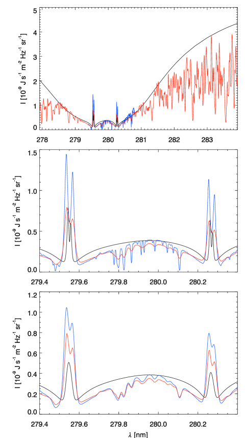
Figure 12.— Comparison of the average spectrum from our 1D computation with RH (black) with observations of solar disk center with the RASOLBA balloon experiment (blue, Staath & Lemaire, 1995) and observations of the quiet sun at disk center during the ninth flight of the HRTS sounding rocket experiment (red, Morrill & Korendyke, 2008). The top panel has a wavelength range including a part of the line wings. The middle and bottom panels show only the h&k line core region. In the bottom panel the RASOLBA and synthetic spectra were convolved to match the spectral resolution of HRTS.

In order to assess whether the synthetic line profiles resemble the Sun we compare them with observations. Observations with spatial resolution comparable to the simulations are not available, so we chose to compare the spatially averaged profile from the simulation to high spectral resolution observations. We emphasize that the goal of this paper is not to reproduce the spatially averaged observed profile, but rather to investigate the sensitivity of spatially resolved Mg II line profiles to variations in the solar atmosphere.

In Figure 12 we show the spatially averaged synthetic Mg II  h&k spectrum from our 1D column-by-column calculation (without microturbulence) with observations of solar disk center with the RASOLBA balloon experiment (Staath & Lemaire, 1995) and quiet sun at disk center with the HRTS9 sounding rocket experiment (Morrill & Korendyke, 2008). The synthetic line profile does not include the blends in the h&k wings, so it is artificially smooth.

Staath & Lemaire (1995) specify that the RASOLBA data were taken at disk center but do not state whether the target region was quiet sun, network, plage or a combination thereof, whereas the HRTS9 observation targeted quiet sun. Because the central emission peaks and the wing intensity in RASOLBA are stronger than in HRTS9, we suspect that the RASOLBA observations included more network or plage than HRTS9.

The synthetic line wings follow the upper envelope of the HRTS9 data quite well up to 283 nm (top panel). For larger wavelengths the synthetic intensity is higher, possibly caused by the neglect of the broad wings of the Mg I line at 285.2 nm in the synthetic spectrum. The middle and lower panels of Figure 12 show the line core region. In the lower panel we smeared the RASOLBA and synthetic spectra to the 20 pm resolution of HRTS9 to make a better comparison. The simulation predicts weaker and narrower emission profiles than observed, but correctly predicts stronger blue peaks and weaker red peaks. The smaller peak separation suggests that the simulation has a weaker velocity field than the Sun. At the resolution of HRTS9, the synthetic red and blue peaks blend into a single peak. The lower peak intensity and integrated emission suggest that the simulation has mid-chromospheric temperature lower than the Sun (see Section 6). Both of these effects may also be related to the magnetic field distribution of the simulation. In Section 9.1 we briefly discuss what is missing in the models. A more extensive investigation of what is missing should await the much higher quality observations that the IRIS mission will provide.

The weaker and narrower mean emission profile from the simulation means that our sample of line profiles most likely cover a more limited range of physical conditions than those that occur in the Sun. Nevertheless, we believe our sample is still extensive enough to cover a good variety of conditions present in at least the quiet Sun.

9. Discussion and conclusions

The Mg II  h&k lines show a complex formation behaviour that spans the entire chromosphere. The variations in temperature, density and velocity in the chromosphere cause a profuse variety of resulting line shapes. Based on statistical-equilibrium non-LTE radiative transfer computations from a snapshot of a 3D radiation-MHD simulation we sought to identify how the Mg II  h&k spectra relate to the underlying atmosphere.

9.1. Limitations of the model atmosphere

We made use of one of the most realistic simulations of the solar chromosphere currently available and modern non-LTE radiative transfer codes that account for partial redistribution effects. Nevertheless, our approach is not without caveats.

The simulation used to compute our model snapshot has some limitations. First, it has a limited spatial resolution. Test computations of simulations with the same domain size but double resolution in each dimension show that higher resolution simulations yield more violent dynamics and significantly more small-scale structure. This is not accounted for in the present paper. Second, we study only one snapshot with one magnetic field configuration. Different field configurations may yield different results. Third, the numerical simulation does not include all physical processes that are important in the chromosphere. Two processes in particular are ignored that have a significant effect on the thermal structure in the chromosphere: non-equilibrium ionization of helium (Leenaarts et al., 2011) and the effect of partial ionization on chromospheric heating by magnetic fields (Khomenko & Collados, 2012; Martínez-Sykora et al., 2012).

A limitation of our radiative transfer calculations is the assumption of statistical equilibrium. This assumption is based on the analysis of the ionization/recombination timescale in Paper I, where we found that in the upper chromosphere this timescale is of the order of 50 s, and much smaller in deeper layers. Our results are therefore not necessarily valid in circumstances where the thermodynamic state of the atmosphere changes over shorter timescales, such as in flares (e.g., Hudson, 2011) and type II spicules (e.g., De Pontieu et al., 2007; Pereira et al., 2012). Computations without the assumption of statistical equilibrium are currently only possible using 1D simulations (Carlsson & Stein, 2002; Rammacher & Ulmschneider, 2003; Kašparová et al., 2009), and therefore lack realism in other areas. Nevertheless it would be interesting to study the response to rapid heating events of the Mg II  h&k lines with time-dependent radiative transfer.

9.2. The k₃ and h₃ intensity minima

The most powerful diagnostic from k₃ and h₃ is their velocity shift. We found it to be tightly correlated with the atmospheric velocity at $z(\tau\!=\!1)$. This correlation could be affected if the temperature in the upper chromosphere is higher in the Sun than in the simulation. The tight correlation depends on the steep optical depth-height gradient, that causes a very narrow height interval with non-zero contribution function. A temperature increase could cause significant ionization to Mg III, and in some cases a corresponding decrease in optical depth-height gradient, and thus a larger formation height range over which the atmospheric velocity is averaged.

The anticorrelation of the k₃ and h₃ intensities and $\tau\!=\!1$ height also offers significant diagnostic potential. The intensity can be used as a measure of the relative height of optical depth unity for locations lying a few Mm or less apart. Combined with the fact that optical depth unity in the intensity minima is typically located less than 200 km below the transition region, they could provide a measure of the local shape of the transition region.

This anticorrelation is likely not qualitatively affected by differences in the upper chromosphere between the Sun and our simulation, because the average radiation field that sets the correlation is not affected by the local temperature. Changes in the temperature around the thermalization depth will change the shape and location in parameter space of the distribution. However, because the intensity can only be used as a relative, and not absolute, height diagnostic this does not affect its usefulness.

9.3. The k₂ and h₂ intensity maxima

The k₂ and h₂ intensities can be used as temperature indicators. Figure 6 illustrates that a strong correlation between peak intensity and temperature at the $\tau\!=\!1$ height exists for radiation temperatures above 6 kK. For radiation temperatures below this value the distributions show a significant amount of scatter, caused by points where the peaks are formed in the upper chromosphere where the source function is decoupled from the local temperature.

For pixels with a good correlation the $\tau\!=\!1$ height cannot be given because of the spread in $\tau\!=\!1$ heights and the presence of multiple-peaked contribution functions (see Figures 9 and 10). Still, we find that a strong emission peak indicates a temperature typically 500 K higher than the peak radiation temperature at some height in the mid-chromosphere. The time variation of the peak intensity can thus be used as an indicator of temperature variations. Note that even the quiet Sun observations show larger average peak intensities than our simulation. It is therefore reasonable to expect that spatially resolved observed spectra will typically have more pixels with high peak intensity for which the intensity-temperature correlation is good than our simulation.

The spatial average of the peak intensity can be used as an observable to test models of the chromosphere. The average peak intensity increases if the temperature in the mid-chromosphere is higher. Large discrepancies between observed and modeled average peak intensity therefore indicate an incorrect temperature structure in the models. They can therefore indicate whether the models include sufficient chromospheric heating and a correct description of the equation of state.

We found that the peak separation is mainly determined by the large-scale velocity gradients in our simulation. The correlation between peak separation and the line-of-sight velocity gradient is good enough that the peak separation can be used both diagnostically as a measure of the velocity structure in the upper chromosphere and as a test of chromospheric models.

The comparison with observations show that the average synthetic peak separation is smaller than observed. We speculate that in the Sun also turbulence at lengths too small to be resolved in our simulation might play a role. An interesting follow-up study would be to investigate peak separation in a series of models with identical parameters but for different spatial resolution, to see how the peak separation changes.

The average Doppler shift of the peaks gives a rough indication of the vertical velocity at the average $\tau\!=\!1$ height of the peaks.

Finally, the intensity peak height ratio is an indication of the average velocity between the peak $\tau\!=\!1$ height and the $\tau\!=\!1$ height of the intensity minimum. This relation is very clear for large intensity ratios: very asymmetric peak heights indicate strong upflows or downflows. This indicates they are suited as a diagnostic of both internetwork acoustic waves, just as Ca II H&K (Carlsson & Stein, 1997), and as diagnostics of compressive waves in more strongly magnetized regions in the solar atmosphere.

9.4. Mg II  h&k and IRIS

So far we studied the Mg II  h&k lines at the native spatial resolution of the simulation and high spectral resolution of the non-LTE radiative transfer computations. IRIS will be equipped with an imaging spectrograph with $<$8 pm spectral resolution and a Mg II k slit-jaw imager with 0.4 nm band pass. Both instruments will have a spatial resolution of $0.\arcsec 4$. The finite resolution of IRIS will influence the diagnostic properties of Mg II  h&k and the correlations derived in the current paper. In forthcoming papers of this series we will quantify these effects and also study the time evolution of synthetic imagery and spectra computed from a time series of 3D radiation-MHD snapshots.

References

- Asensio Ramos et al. (2008) Asensio Ramos, A., Trujillo Bueno, J., & Landi Degl’Innocenti, E. 2008, ApJ, 683, 542
- Asplund et al. (2009) Asplund, M., Grevesse, N., Sauval, A. J., & Scott, P. 2009, ARA&A, 47, 481
- Carlsson & Leenaarts (2012) Carlsson, M. & Leenaarts, J. 2012, A&A, 539, A39
- Carlsson & Stein (1994) Carlsson, M. & Stein, R. F. 1994, in Chromospheric Dynamics, ed. M. Carlsson, 47
- Carlsson & Stein (1997) Carlsson, M. & Stein, R. F. 1997, ApJ, 481, 500
- Carlsson & Stein (2002) Carlsson, M. & Stein, R. F. 2002, ApJ, 572, 626
- Cauzzi et al. (2009) Cauzzi, G., Reardon, K., Rutten, R. J., Tritschler, A., & Uitenbroek, H. 2009, A&A, 503, 577
- de la Cruz Rodríguez et al. (2012) de la Cruz Rodríguez, J., Socas-Navarro, H., Carlsson, M., & Leenaarts, J. 2012, A&A, 543, A34
- De Pontieu et al. (2007) De Pontieu, B., McIntosh, S., Hansteen, V. H., et al. 2007, PASJ, 59, 655
- Gudiksen et al. (2011) Gudiksen, B. V., Carlsson, M., Hansteen, V. H., et al. 2011, A&A, 531, A154
- Hayek et al. (2010) Hayek, W., Asplund, M., Carlsson, M., et al. 2010, A&A, 517, A49
- Hudson (2011) Hudson, H. S. 2011, Space Sci. Rev., 158, 5
- Kašparová et al. (2009) Kašparová, J., Varady, M., Heinzel, P., Karlický, M., & Moravec, Z. 2009, A&A, 499, 923
- Khomenko & Collados (2012) Khomenko, E. & Collados, M. 2012, ApJ, 747, 87
- Leenaarts & Carlsson (2009) Leenaarts, J. & Carlsson, M. 2009, in Astronomical Society of the Pacific Conference Series, Vol. 415, Astronomical Society of the Pacific Conference Series, ed. B. Lites, M. Cheung, T. Magara, J. Mariska, & K. Reeves, 87
- Leenaarts et al. (2011) Leenaarts, J., Carlsson, M., Hansteen, V., & Gudiksen, B. V. 2011, A&A, 530, A124
- Leenaarts et al. (2007) Leenaarts, J., Carlsson, M., Hansteen, V., & Rutten, R. J. 2007, A&A, 473, 625
- Leenaarts et al. (2012) Leenaarts, J., Carlsson, M., & Rouppe van der Voort, L. 2012, ApJ, 749, 136
- Martínez-Sykora et al. (2012) Martínez-Sykora, J., De Pontieu, B., & Hansteen, V. 2012, ApJ, 753, 161
- Morrill et al. (2001) Morrill, J. S., Dere, K. P., & Korendyke, C. M. 2001, ApJ, 557, 854
- Morrill & Korendyke (2008) Morrill, J. S. & Korendyke, C. M. 2008, ApJ, 687, 646
- Nordlund (1982) Nordlund, A. 1982, A&A, 107, 1
- Pereira et al. (2012) Pereira, T. M. D., De Pontieu, B., & Carlsson, M. 2012, ApJ, 759, 18
- Rammacher & Ulmschneider (2003) Rammacher, W. & Ulmschneider, P. 2003, ApJ, 589, 988
- Reardon et al. (2009) Reardon, K. P., Uitenbroek, H., & Cauzzi, G. 2009, A&A, 500, 1239
- Rezaei et al. (2008) Rezaei, R., Bruls, J. H. M. J., Schmidt, W., et al. 2008, A&A, 484, 503
- Sekse et al. (2012) Sekse, D. H., Rouppe van der Voort, L., & De Pontieu, B. 2012, ApJ, 752, 108
- Skartlien (2000) Skartlien, R. 2000, ApJ, 536, 465
- Staath & Lemaire (1995) Staath, E. & Lemaire, P. 1995, A&A, 295, 517
- Stenflo (1994) Stenflo, J. 1994, Solar Magnetic Fields: Polarized Radiation Diagnostics, Astrophysics and Space Science Library (Springer)
- Uitenbroek (2001) Uitenbroek, H. 2001, ApJ, 557, 389
- Uitenbroek (2011) Uitenbroek, H. 2011, in Astronomical Society of the Pacific Conference Series, Vol. 437, Solar Polarization 6, ed. J. R. Kuhn, D. M. Harrington, H. Lin, S. V. Berdyugina, J. Trujillo-Bueno, S. L. Keil, & T. Rimmele, 439
- Štěpán et al. (2012) Štěpán, J., Trujillo Bueno, J., Carlsson, M., & Leenaarts, J. 2012, ApJ, 758, L43