The formation of IRIS diagnostics
I. A quintessential model atom of MG II and general formation properties of the MG II H&K lines

Abstract

NASA’s Interface Region Imaging Spectrograph (IRIS) space mission will study how the solar atmosphere is energized. IRIS contains an imaging spectrograph that covers the Mg II  h&k lines as well as a slit-jaw imager centered at Mg II k. Understanding the observations will require forward modeling of Mg II  h&k line formation from 3D radiation-MHD models. This paper is the first in a series where we undertake this forward modeling. We discuss the atomic physics pertinent to h&k line formation, present a quintessential model atom that can be used in radiative transfer computations and discuss the effect of partial redistribution (PRD) and 3D radiative transfer on the emergent line profiles. We conclude that Mg II  h&k can be modeled accurately with a 4-level plus continuum Mg II model atom. Ideally radiative transfer computations should be done in 3D including PRD effects. In practice this is currently not possible. A reasonable compromise is to use 1D PRD computations to model the line profile up to and including the central emission peaks, and use 3D transfer assuming complete redistribution to model the central depression.

1. Introduction

Magnesium is one of the most abundant elements in the solar atmosphere and as such its neutral and singly ionized state give rise to a number of spectral lines with significant diagnostic potential in the photosphere as well as in the chromosphere. Well-known examples are the Mg I 457.1 nm forbidden line, which is a photospheric temperature diagnostic, the Mg I b lines around 517 nm, which serve as upper photospheric/lower chromospheric magnetic field diagnostics, the Mg I 12 $\mu$m infrared lines, which exhibit very peculiar Non-LTE radiative transfer behavior (Chang et al., 1991; Carlsson et al., 1992), the 285.2 nm Mg I resonance line, which shows effects of partial frequency redistribution (PRD, Uitenbroek & Briand, 1995), and finally the Mg II  h&k resonance doublet at 280.27 and 279.55 nm, respectively. The latter two lines are among the strongest, and therefore potentially most valuable diagnostically, in the solar spectrum, but have rarely been observed because of their wavelength in the middle of the UV range, precluding ground based observation.

This situation will change drastically with the NASA Interface Region Imaging Spectrograph (IRIS) spacecraft, which will be equipped with a high resolution UV imaging spectrograph ($<$80 mÅ spectral resolution) and Mg II k slit-jaw imager (4 Å filter width) with $0\arcsec.4$ spatial resolution.

Previously, disk center calibrated intensities have been obtained with the Hawaii (Allen & McAllister, 1978) and Harvard (Kohl & Parkinson, 1976) sounding rocket experiments. Low temporal and spatial resolution ($2\arcsec$), but high spectral resolution (20 mÅ) spectra have been obtained with the Ultraviolet Spectrometer and Polarimeter (UVSP, Woodgate et al., 1980) instrument on board the Solar Maximum Mission (SMM, Vial, 1984). The lines have been observed simultaneously with other chromospheric spectral lines in the UV (Lyman $\alpha$ and $\beta$, and the Ca II H&K lines) by the LPSP instrument on board the OSO 8 mission (Bonnet et al., 1978; Artzner et al., 1978; Vial et al., 1979; Kneer et al., 1981; Vial et al., 1981) Spatially resolved spectra of the Mg I 285.2 nm (Uitenbroek & Briand, 1995) and Mg II  h&k lines were obtained with the French balloon experiment RASOLBA (Staath & Lemaire, 1995) , and the sounding rocket experiment HRTS on its ninth flight (Morrill & Korendyke, 2008), both on photographic film. Polarimetric observations in the h&k lines were obtained with two flights of the Solar Ultra-violet Magnetograph Investigation (SUMI, West et al., 2011) sounding rocket experiment.

Because magnesium is about 18 times more abundant than calcium (Asplund et al., 2009) the h&k lines form correspondingly higher in the solar atmosphere than the homologous Ca II H&K lines. From the sparse observations described above it is clear that the magnesium resonance lines sample a different regime of the solar atmosphere than the H&K lines, which regularly lack emission reversals altogether, or exhibit singly-peaked profiles (Rezaei et al., 2008), whereas the former lines always have doubly-peaked emission reversals, except in sunspots (Morrill et al., 2001). In addition, the strong red-blue asymmetry of the Ca II H&K lines that is thought to be the result of acoustic waves steepening into shocks (Carlsson & Stein, 1997) is much less pronounced in the h&k lines (Gouttebroze, 1989). Since the magnetic network gives rise to more symmetric and less intermittent Ca II H&K line profiles, the question arises if the magnetic field also gives rise to the omnipresent emission reversals in the h&k lines, or whether the different morphology of the emission in the latter lines can be explained by the same dynamic effects that cause the intermittent Ca II behavior, given that the magnesium lines sample a different height due to their larger opacity.

Slight differences in atomic structure between singly ionized calcium and magnesium create an interesting opportunity for simultaneous temperature and velocity diagnostics in the spectral window sampled by the IRIS spectrograph. Whereas the Ca II $3d\,^{2}\!D$ levels have a lower energy by about 1.3 eV than the $4p\,^{2}\!P$ upper levels of the H&K lines, and thus allow for the $4d\,^{2}\!D$ – $4p\,^{2}\!P$ triplet to form in the infrared, the Mg II $3d\,^{2}\!D$ levels lie at about the same energy difference above the $3p\,^{2}\!P$ levels as these levels lie above the Mg II $3s\,^{2}\!S$ ground state. As a result the $3d\,^{2}\!D$ – $3p\,^{2}\!P$ triplet forms in the UV, very close to the h&k resonance lines, overlapping with them in wavelength.

Because of their high opacity (magnesium is almost exclusively in its singly ionized state as shown in Sec. 6.2) radiation in the Mg II resonance and $3d\,^{2}\!D$ – $3p\,^{2}\!P$ triplet emanates from in the low-density chromosphere, where non-LTE radiative transfer and effects of PRD are crucial to line formation. Previously, the Mg II lines had been modeled with PRD in one-dimensional fashion and compared with observations by Milkey & Mihalas (1974), Uitenbroek (1997), and Gouttebroze (1989), among others. Inversion of the spectra that the IRIS mission will provide into physical quantities is therefore a complicated endeavor and is best achieved by comparing forward modeling of spectra through numerical simulations of a radiation magneto-hydrodynamics (RMHD) with observations, and using such simulations to extract what observable quantities mean in terms of physical quantities of the underlying atmosphere. In this paper we therefore present a new updated study of the line formation properties of the Mg II  h&k lines incorporating the latest advances in numerical modeling of the solar chromosphere and non-LTE radiative transfer to help interpretation of IRIS data. To do so we use the same snapshot of a radiation-MHD simulation as Leenaarts et al. (2012a), who studied the formation of the H $\alpha$ line. The reader is encouraged to compare their results with the results for Mg II  h&k in the current paper.

In Section 2 we describe the atomic data that we use to construct our Mg II model atom. Section 3 describes the model atmospheres we use, Section 4 describes the employed radiative transfer codes. In Section 5 we investigate the importance of non-equilibrium ionisation of magnesium, in Section 6 we describe the construction of our quintessential model atom, i.e., the smallest model atom that accurately reproduces the h&k line, in Sections 7–11 we describe the basic h&k line formation properties in some detail, and we finish with our discussion and conclusions in Section 12.

2. Atomic data

We use the magnesium abundance of $A_{\mathrm{Mg}}=7.60\pm 0.04$ on the standard logarithmic scale for abundances where $A_{\mathrm{H}}=12$ from Asplund et al. (2009). These authors remark that there is no agreement between abundance determinations from different lines, and the stated abundance is a straight mean of the abundance determinations for many lines computed of Mg I and Mg II in non-LTE using 1D model atmospheres (Zhao et al., 1998; Abia & Mashonkina, 2004).

The atomic energy levels are taken from the NIST database (Ralchenko et al., 2011).

The oscillator strengths and photo-ionization cross sections are taken from from the TOPbase database (Cunto et al., 1993). Note that some of the photo-ionization cross-sections provided by TOPbase extend below the ionization threshold energy. These data points are added for the purpose of average opacity computations, but should be discarded for non-LTE radiative transfer computations as in this paper (Mendoza, 2012, private communication).

Excitation by collisions with electrons is treated with data from Sigut & Pradhan (1995). Collisional excitation and de-excitation between the h&k upper levels by collisions with neutral hydrogen is included according to Monteiro et al. (1988). These authors give tabulated values up to 5000 K, we use a linear extrapolation above this temperature.

Auto-ionization, collisional ionization from the ground state by electrons and charge exchange with protons and neutral hydrogen are done using the recipes by Arnaud & Rothenflug (1985).

Dielectronic recombination is treated according to Shull & van Steenberg (1982) and collisional ionization from excited states is computed using the procedure of Burgess & Chidichimo (1983).

Broadening of the Mg II  h&k lines by collisions with neutral hydrogen is treated with the formalism of Anstee & O’Mara (1995) using the pertinent coefficients from Barklem & O’Mara (1998).

When we discuss the effect of inclusion of Mg I in the atomic model on the emergent intensity from the Mg II  h&k lines, we use a model atom including Mg I, Mg II and the ground state of Mg III. This atom is created by adding the Mg I model atom of Carlsson et al. (1992) to our Mg II model.

3. Model atmospheres

In this paper we use a number of different model atmospheres. One is the semi-empirical model C from Fontenla et al. (1993). This is a one-dimensional time-independent atmosphere, constructed to match spatially and temporally averaged observed spectra in the UV. This atmosphere is used as a starting point in understanding h&k line formation in a simple, static case. This understanding can then be used in the analysis of more complicated model atmospheres. We henceforth refer to this model as FALC.

The second model is a snapshot of a 3D RMHD simulation performed with the Bifrost code (Gudiksen et al., 2011). The same snapshot has been used by Leenaarts et al. (2012a) to investigate H $\alpha$ line formation.

Bifrost solves the equations of resistive MHD on a staggered Cartesian grid including a variety of physical processes. The simulation we use here included optically thick radiative transfer in the photosphere and low chromosphere (Nordlund, 1982; Skartlien, 2000; Hayek et al., 2010), parametrized radiative losses in the upper chromosphere, transition region and corona (Carlsson & Leenaarts, 2012), thermal conduction along magnetic field lines (Gudiksen et al., 2011) and an equation of state that includes the effects of non-equilibrium ionization of hydrogen (Leenaarts et al., 2007).

The simulation covers a physical extent of $24\times 24\times 16.8$ Mm, with a grid of $504\times 504\times 496$ cells, covering the upper convection zone, photosphere, chromosphere and the lower corona. The horizontal grid spacing is 48 km, the vertical grid spacing is non-uniform, with a spacing of 19 km between $z=-1$ and $z=5$ Mm, and increasing towards the bottom and top of the computational domain. The simulation contains a magnetic field with a an average unsigned strength of 50 G in the photosphere, concentrated in the photosphere in two clusters of opposite polarity. We shall refer to the snapshot from this simulation as 3DMHD.

We also use a snapshot from a 2D simulation performed with Bifrost by Leenaarts et al. (2011). This simulation was performed with the same physics as 3DMHD, but had a very weak magnetic field (0.3 G average unsigned flux in the photosphere). It has a grid size of $325\times 512$ points, with a horizontal grid spacing of 32.5 km spanning 16.6 Mm and a non-uniform vertical grid with a spacing of 28 km between the bottom of the computational domain and $z=5$ Mm, and increasing towards the top of the computational domain to 150 km.

Characteristic of this 2D simulation is that it contains large bubbles of low temperature ($<2000$ K) gas in the chromosphere, which do not occur in 3DMHD. At these low temperatures we expect a significant amount of magnesium in the form of Mg I, so we use the 2D simulation to extend the range of physical circumstances under which we study Mg II  h&k line formation. We call this snapshot 2DMHD.

4. Radiative transfer

We perform non-LTE radiative transfer computations with two different codes. The first is a modified version of RH by Uitenbroek (2001). This version was parallelized using MPI so it can efficiently solve the radiative transfer in all columns in a 3D model atmosphere assuming each column is a plane-parallel 1D atmosphere. It can treat the effects of angle-dependent partial frequency redistribution (PRD) using the fast approximation by Leenaarts et al. (2012b). We employ a non-constant coherency fraction $\gamma$, given by

$$\gamma=\frac{P_{j}}{P_{j}+Q^{\mathrm{E}}_{j}},$$ (1)

where $P_{j}$ is the total (collisional and radiative) rate out of the upper level of the transition $j$ and $Q^{\mathrm{E}}_{j}$ is the rate of elastic collisions for the upper level. For further details on the treatment of PRD we refer to Uitenbroek (2001).

The second code we use is Multi3d (Leenaarts & Carlsson, 2009). This is an MPI-parallelized radiative transfer code that can evaluate the radiation field in full 3D, taking the horizontal structure in the model atmosphere into account. The current iterative solution methods for non-LTE radiative transfer with PRD effects are not stable enough to include in 3D. Our computations with Multi3d are done assuming complete redistribution (CRD). This assumption gives wrong line intensities from the wings up to and including the line core emission peaks (k₂ and h₂). However, we show in Section 10 that the central line depressions (k₃ and h₃) are only weakly affected by PRD.

For the FALC model we add additional spectral line broadening using the height-dependent microturbulent velocity given in Fontenla et al. (1991). Computations using the 3DMHD and 2DMHD atmospheres do not use microturbulence.

Summarizing, we model the h and k lines in 1D including PRD with the RH code, and in 3D assuming CRD with Multi3d. Ideally one should perform 3D computations including PRD, but this is currently beyond our capabilities.

5. Non-equilibrium ionization

Hydrogen ionization is out of equilibrium in the dynamic solar chromosphere due to long ionization/recombination time-scales compared with dynamical timescales (Carlsson & Stein, 2002; Leenaarts et al., 2007). If the same is true for magnesium, it would be necessary to take into account the history of the atmosphere when interpreting Mg II spectra.

We here investigate the timescales of ionization/recombination of Mg II-Mg III using the same methodology as in Carlsson & Stein (2002). We use a time-series of 1D hydrodynamical snapshots computed with RADYN (e.g., Carlsson & Stein, 1992, 1997). This code self-consistently solves the equations of conservation of mass, momentum, energy and charge together with the non-LTE rate equations for hydrogen, helium and calcium. The equations are formulated on an adaptive grid (Dorfi & Drury, 1987) that ensures high numerical resolution where the gradients are large (e.g., in shock fronts). We use the same time-series as in Carlsson & Stein (2002) and refer the reader to that paper for details on the numerical implementation.

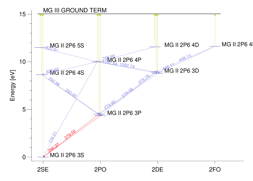
Figure 1.— Term diagram of the 10-level plus continuum Mg II atomic model. The Mg II  h&k lines are indicated by red lines, all other bound-bound transitions are blue, the bound-free transitions are yellow. All lines indicating bound-bound transitions are annotated with the line-center wavelength in nm.

For each snapshot in the time-series we perturb the atmosphere by increasing the temperature by 1% and calculate the time evolution of the population densities. We use a 10-level plus continuum model atom for Mg II. Its term diagram is given in Fig. 1. We determine the timescale for ionization/recombination by fitting the time evolution of the Mg III population density with the analytic solution for a two-level atom:

$$n(t)=n(\infty)+(n(0)-n(\infty)){\rm e}^{-t/t_{\rm relax}},$$

where $n(t)$ is the population density at time $t$, $n(\infty)$ is the equilibrium population density of the perturbed atmosphere, $n(0)$ is the population density of the initial atmosphere and $t_{\rm relax}$ is the timescale for relaxation to the final state.

Figure 2 shows the relaxation time and the temperature as function of column mass. The relaxation time increases from milliseconds in the photosphere to about 50 seconds at the top of the chromosphere. Note, however, that this dynamic simulation starts from a radiative equilibrium atmosphere and it thus has a low temperature in the chromosphere apart from when shocks travel through. In the shocks, the relaxation time is lowered by one order of magnitude compared with the pre-shock, low temperature state (e.g.,  at $t=1760$s when there is a shock at $\lg(m_{c})=-3.7$). In the transition region, the relaxation timescale drops to fractions of a second. We conclude that whenever the temperature is high enough to give a significant fraction of Mg III, the relaxation time is short and statistical equilbrium is a good approximation for magnesium.

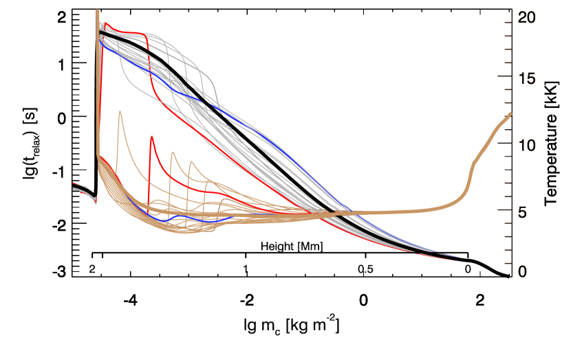
Figure 2.— Relaxation timescale (grey/black, left axis) and gas temperature (brown, right axis) as function of column mass and time in the dynamic simulation at 10s intervals from $t=1600$s to $t=1780$s. The thickest lines represent the relaxation timescale and the temperature averaged in time over all time steps between $t=1120$s and $t=3590$s. Two individual time steps are drawn as thick lines: $t=1640$s (red) and $t=1760$s (blue). The height scale of the initial state is given as reference.

6. Quintessential model atom

In this section we investigate the effect of the size of the model atom on the emergent Mg II  h&k line profiles.

6.1. Starting atom

As a starting atomic model for Mg II we use the same 10-level plus continuum model atom as in Section 5. Its term diagram is given in Fig. 1. The h&k lines at 279.55 nm and 280.27 nm are lines from the $3s\,^{2}\!S$ ground state to the $3p\,^{2}\!P$ excited states. There is a triplet of lines between the $3p\,^{2}\!P$ and $3d\,^{2}\!D$ states with wavelengths close to the h&k lines. One has a wavelength of 279.08 nm and is located on the blue side of the k core, The other two are overlapping lines at 279.79 nm and 279.80 nm and are located in between the h&k line cores. This triplet can potentially be used as an upper-photospheric/low-chromospheric velocity indicator. We plan to investigate the diagnostic value of the triplet in a future paper. The 4d, 4p and 4f terms are merged into single levels. Their energy is computed as an average of the energy of the levels in the term, weighted with their statistical weight.

6.2. Importance of Mg I

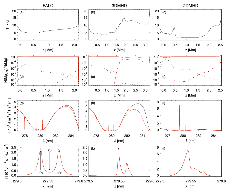
Figure 3.— Comparison between the Mg II model atoms with Mg I treated consistenlty in non-LTE and treated as an LTE source of background opacity in three different plane parallel atmospheres (FALC, left-hand column, 3DMHD, middle column and 2DMHD, right-hand column). Black curves always show quantities for the atom including non-LTE Mg I, red curves when Mg I is included as LTE background opacity. Panels (a)–(c) show the temperature structure as function of height in the atmosphere. Panels (d)–(f) display the fraction of all Mg atoms in the form of Mg I (dotted), Mg II (solid) and Mg III(dashed). Dashed: upper level of the k line. Dotted: upper level of the h line. Panels (g)–(i) show the vertically emergent intensity in the entire profile. Panels (j)–(l) show the vertically emergent intensity in the core of the k line. In panel (j) we show the commonly used names of the features in the line core profile. The central depression is called k₃, the emission peak on the short-wavelength (blue) side of the depression is called k_2V, the peak on the red side is called k_2R.

A fraction of all magnesium atoms in the solar atmosphere is in the form of Mg I. The ionization balance is sensitive to the temperature and electron density, through the Saha-equation in LTE and the ionization and recombination rate coefficients in non-LTE (cf. Mihalas, 1978; Rutten, 2003). It is thus expected that the fraction of magnesium in its neutral form is highest in cool gas at a high density.

The addition of Mg I levels to our Mg II model atom causes a large performance penalty due to the large increase in the number of levels and transitions. This penalty is so large that it would hamper computation of the h&k lines from time-series of large 3D radiation-MHD simulations.

We therefore investigated whether Mg I should be included in non-LTE for accurate computation of the h&k line profiles. We created a model atom including neutral, singly ionized and twice ionized magnesium by adding the 65-level Mg I atom of Carlsson et al. (1992) to the Mg II model, including all pertinent transitions.

We then compared the non-LTE radiative transfer problem between this large model atom, and our small 10-level plus continuum Mg II atom where we only included the 65-level Mg I atom as a source of background opacity assuming LTE. Including Mg I in LTE in the background does not significantly increase the amount of computational work.

We used RH to solve the radiative transfer problem for both model atoms in three plane-parallel atmospheres: FALC, a column of 3DMHD and a column of 2DMHD. From the latter model we specifically chose a column with a low temperature throughout most of the chromosphere and photosphere, thus representing a case with a large influence of Mg I on the h&k profiles.

The results are shown in Fig. 3. Panels (a)–(c) show the temperature structure in the models, panels (d)–(f) show the fraction of all magnesium in the various ionization states. As expected, the fraction of Mg I is largest in cool areas in the photosphere, but only in the extremely cool 2DMHD case it exceeds 10%. Above 1 Mm height at most 1% of magnesium is in the form of neutral atoms.

Panels (g)–(o) show the effect on the emergent line profiles. If Mg I is treated as an LTE background element, then the opacity in the wavelength range of the h&k lines is increased owing to the larger fraction of Mg I in LTE compared to non-LTE. In the h&k line cores the Mg I opacity is insignificant. In the outer line wings however, Mg I opacity is important, especially in the red wing of Mg II h because of the presence of the Mg I resonance line at 285.2 nm.

Treating Mg I in LTE leads to higher wing opacity. With a source function that decreases with height this results in a lower h&k wing intensity. The cores of the lines are, however, completely unaffected.

We therefore conclude that it is safe to ignore Mg I if one is interested mainly in the chromosphere where the h&k line cores are formed. If one is interested in precise computation of the outer line wing intensity, then Mg I should be included in non-LTE. Note that the line wings are blended with many lines, mainly from iron, which then also should be included. We focus here mainly on the properties of h&k line formation relevant for the IRIS mission, so we ignore Mg I for the remainder of this paper.

6.3. Influence of number of levels in the Mg II atom

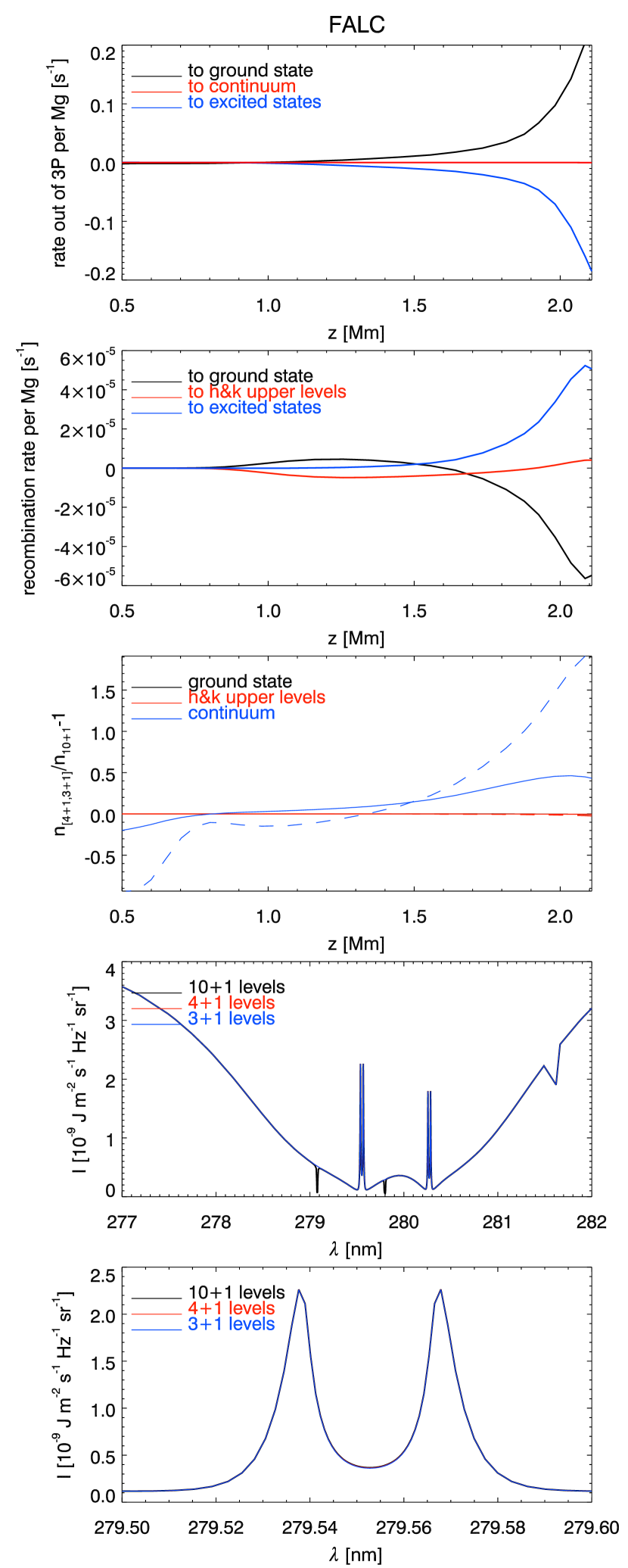
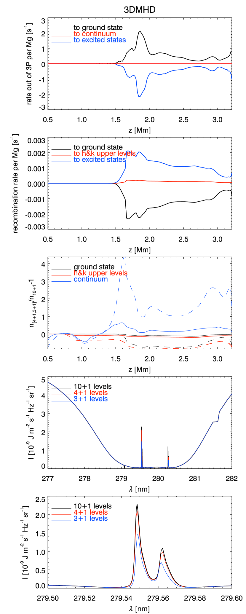
Figure 4.— Analysis of the transition rates between levels in the 10+1 level Mg II model atom in the FALC model (left) and a column of 3DMHD (right), the same column as in Fig. 3. First row: net transition rate out of the h&k upper level. Second row: net recombination rate to various bound levels. Third row: relative difference in population with respect to the 10+1 level reference atom for the 4+1 level atom (solid) and the 3+1 level atom (dashed). Fourth row: emergent intensity in the h&klines for the various model atoms. Fifth row: emergent intensity in the line core of the k line for the various model atoms.

The 10-level plus continuum Mg II atom contains 15 bound-bound and 10 bound-free radiative transitions. Especially for 3D computations it would be beneficial to construct a model atom with fewer levels and transitions to speed up computations. To do so we investigated the various rates in our 10+1 level magnesium atom and show the results of this analysis in Fig. 4 for the FALC model (left-hand column) and a column of 3DMHD (right-hand column).

The top row shows the net rate $P_{\mathrm{net}}$ out of the h&k upper levels ($3p\,^{2}\!P$ states):

$$P_{\mathrm{net}}=\frac{1}{n_{\mathrm{Mg}}}\sum_{i}\sum_{j}\left(n_{i}P_{ij}-n_{j}P_{ji}\right),$$ (2)

where the $i$ summation is over the two upper levels of h&k, and the summation over $j$ is over the target states, $n_{\mathrm{Mg}}$ is the total density of magnesium atoms, $n_{i}$ is the population of level $i$ and $P_{ij}$ is the total (collisional plus radiative) rate from level $i$ to level $j$. In the deepest part of the atmosphere the h&k lines are in detailed balance, but towards the top of the atmosphere the h&k upper levels are populated from the higher-lying excited bound states and depopulated to the ground state. The rate to the continuum is negligible.

The second row shows the net recombination rate to the various bound levels. Here the situation is more complex. In FALC below $z=1.5$ Mm recombination is to the ground state, and ionization is from the h&k upper levels. Above 1.5 Mm the situation is different, there ionization is from the ground state, and recombination is to the higher-lying excited bound states. The same holds for the 3DMHD column.

In conclusion, the h&k lines are effectively in detailed balance from the photosphere up to the mid chromosphere. In the upper chromosphere, where the line core forms, h&k are part of an ionization/recombination loop, where recombination occurs through the highly excited levels, followed by a cascade down through the h&k lines to the ground state after which ionization occurs again.

We then proceeded to study the differences that occur with smaller model atoms.

We created the simplest model atom capable of reproducing the h&k lines, which is a 3-level plus continuum atom, with the ground state and the two $3p\,^{2}\!P$ states. However, this atom cannot support the ionization/recombination loop described above.

The smallest model atom that can support the loop is a 4-level plus continuum atom, the same as the 3+1 level atom, but with an artificial level included that mimics the effect of the excited states above the $3p\,^{2}\!P$ states. This level was created by merging all these excited states so that the total rates in and out of the levels are roughly conserved in the new merged level. Its energy is the average of all the merged levels weighted with their statistical weight.

We then solved the radiative transfer of these 3+1 and 4+1 level atoms for the same two models, and plot the relative population difference with the 10+1 level atom in the third row of Fig. 4. In FALC the h&k upper and lower level populations are unchanged, but the population of the continuum is very different. As expected, the 4+1 level atom does a better job than the 3+1 level atom in reproducing the full atomic model populations. In 3DMHD the situation is very different. The 3+1 level atom has too low h&k upper and lower level populations, leading to a too low opacity, and a different ratio of the upper and lower level populations, leading to a different source function. The 4+1 level atom does a much better job in reproducing the populations from the full atom.

This is further demonstrated in the fourth row of Fig. 4 which shows the emergent intensity for the three different model atoms in the h&k lines, and the fifth row, which shows the core of the k line. The line wings are nearly identical, but the 3+1 level atom fails to reproduce the 10+1 level atom line core in 3DMHD. In contrast, the 4+1 level atom does a very good job, with only a slight difference in the k_2V and k_2R peak intensity.

We compared the absolute value of the relative difference in emergent intensity between the 3+1 and 4+1 level atom and the 10+1 atom for a $yz$-slice through the 3DMHD snapshot. The 4+1 level atom has a maximum average deviation of 3%. Inspection of all individual columns in the slice shows that the difference in any given column is never larger than 11%, whereas the 3+1 level atom shows differences larger than 50%

We conclude that it is possible to accurately model the h&k lines with a 4+1 level model atom. Further simplification to a 3+1 level atom leads to significant errors in the line core intensity.

7. Broadening in the h&k lines

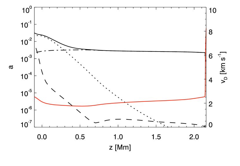
Figure 5.— Voigt $a$ damping parameter and Doppler width $\sqrt{2kT/m}$ for the Mg II k line in the FALC atmosphere. The total damping is shown in solid black (left-hand scale) with the contributions from radiative damping (dash-dotted), Van der Waals broadening (dotted) and the quadratic Stark effect (dashed). The Doppler width is shown in solid red (right-hand scale).

In this section we discuss the various broadening mechanisms of the h&k lines. We investigate only the k line, as the h line behaves nearly identically. Fig. 5 shows the various contributions to the damping and the Doppler width of the k line in the FALC model.

The h&k lines are resonance lines, the radiative damping is the largest contribution to the total damping in the chromosphere ($z>500$ km). Van der Waals broadening is the dominant contribution in the photosphere. Quadratic Stark broadening is only of minor importance. The Voigt $a$ parameter varies from $2.5\times 10^{-3}$ in the chromosphere to $2.5\times 10^{-2}$ in the photosphere. The h&k lines have very broad wings due to their large opacity in the photosphere. In the FALC model, the combined h&k line opacity at $z=200$ km becomes equal to the continuum opacity at 277.25 nm and 282.34 nm, more than 2 nm away from the nearest h&k line-center frequency. However, the theoretical continuum intensity is never reached in a solar spectrum. The haze of overlapping UV lines prevents the intensity of reaching the ‘true’ continuum (Lemaire & Samain, 1989).

Magnesium has an atomic weight of 24.3 u, and a corresponding Doppler width $\sqrt{2kT/m}$ between 2 and 3 km s^-1 for typical chromospheric temperatures.

8. Coupling between h&k upper levels and the relative height of the emission peaks

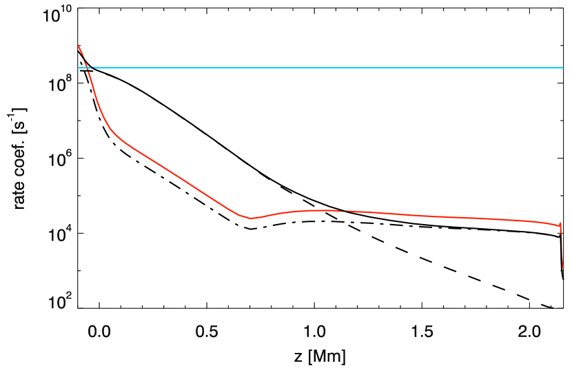
Figure 6.— Transition rate coefficients out of the upper level of the Mg II k line in the FALC atmosphere. Solid black: total collisional rate coefficient to the upper level of the Mg II h  line, with contribution due to collisions with neutral hydrogen (dashed) and electrons (dot-dashed). For comparison the radiative rate coefficient to the ground state (blue) and the collisional rate coefficient to the ground state (red) are also shown.

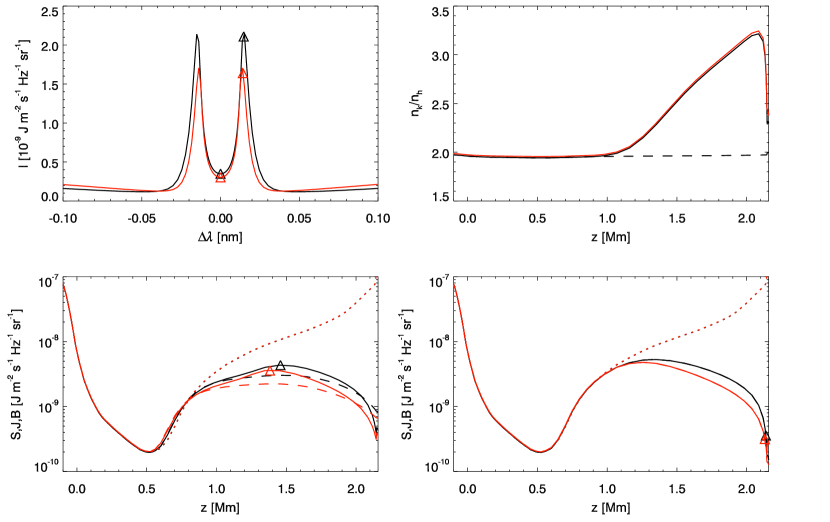
Figure 7.— Difference in emission peak height between the h&k lines in the FALC model atmosphere. The triangles indicate wavelengths analyzed in the lower panels. Upper left: h (red) and k (black) line core profiles as function of wavelength shift away from line center. Upper-right: ratio of the h&k upper level populations $n_{\mathrm{k}}/n_{\mathrm{h}}$ in non-LTE (solid black) and LTE (dashed black). The ratio of the upward radiative rates $R_{\mathrm{k}}/R_{\mathrm{h}}$ is overplotted in red. Lower-left: source function (solid), angle-averaged radiation field (dashed) and Planck function (dotted) at the red emission peak (indicated by the triangles in the upper-left panel) for the k line (black) and the h line (red). The triangles indicate optical depth unity at this wavelength. Lower-right: same as lower left, but now for line-center.

Because of the small energy difference between the h&k upper levels, inelastic collisions with neutral hydrogen are important for the transition rates between these levels, in addition to collisions with electrons. In the photosphere and lower chromosphere the collisions with neutral hydrogen are more important than collisions with electrons due to the low ionization degree of hydrogen there. This is demonstrated in Fig. 6, which compares various rate coefficients out of the upper level of the Mg II k line in the FALC atmosphere. Collisional de-excitation to the Mg II h upper level by neutral hydrogen is dominant between 0 Mm and 1.1 Mm height, above 1.1 Mm de-excitation by electrons dominates. For comparison we show the collisional de-excitation to the ground state (red), which is comparable to the de-excitation to the Mg II h upper level. In addition we show the radiative de-excitation to the ground state (blue), which is orders of magnitude larger than the collisional rates, illustrating that Mg II k is strongly scattering. The fact that the collisional rates between the levels are much smaller than the spontaneous radiative de-excitation rate to the ground state means that the h&k upper levels are only weakly coupled with each other and significant differences in the source function can be expected. This is indeed the case, the k line typically has stronger emission peaks than the h line in both observations (e.g., Tousey, 1967) and theoretical calculations. Interestingly the observations also show a larger peak height ratio in plage than in quiet sun, indication a sensitivity to the temperature structure in the atmosphere.

The Ca II H&K lines show a similar effect, which was explained by Linsky (1970). In short, the Ca II K has twice the opacity as the H line, and hence its source function thermalizes at a slightly larger height than the source function of the H line. This means that in a chromosphere with an outwardly increasing temperature the K source function follows the temperature rise more strongly than the H line, and hence the K emission peaks are higher.

Linsky & Avrett (1970) argued that the Mg II  h&k lines should behave qualitatively the same as Ca II H&K. We confirm this by analyzing the formation difference between h&k in the FALC atmosphere in Fig. 7. The upper-left panel shows the h&k line profiles, with a higher emission-peak intensity for the k line. The upper right panel shows the ratio of the non-LTE upper level populations, indicating that the k line has a higher source function $S$ because (neglecting PRD effects) $S_{k}/S_{h}\approx{1\over 2}n_{k}/n_{h}$ as the lines share a common lower level and the ratio of the statistical weights of the upper levels is 2 (Rutten, 2003, Sect 2.6.2). The near equality of the population ratio with the ratio of the radiative rates in the h&k lines shows that the populations are set completely by the line radiation. The lower panels finally show a comparison of the source function and height of optical depth unity. Because the k opacity is twice as high as the h opacity, optical depth unity in the emission peaks in the k line is reached already at larger heights, and the source function is larger (lower-left panel). This leads to the larger emission peak height. The k-line source function is also higher around optical depth unity at line center, leading to a larger line-center intensity.

9. Effect of optical pumping by H I Ly $\beta$

The Mg II atom has two radiative transitions between the $5p\,^{2}\!P$ states and the $3s\,^{2}\!S$ ground state, at wavelengths close to 102.6 nm, which is in the red wing of the H I Ly $\beta$ line. Optical pumping in these transitions from the ground state through the large radiation field caused by the Lyman line could influence the formation of the h&k lines by creating a pathway for population of the h&k upper levels.

We investigated this effect by computing the simultaneous non-LTE solution of a five level plus continuum H I and a 21-level plus continuum Mg II atom with and without these two transitions in the FALC atmosphere and one column from the 3DMHD snapshot. In both cases neglecting the $3s\,^{2}\!S$ – $5p\,^{2}\!P$ transitions has a negligible effect on the h&k lines.

10. Importance of 3D radiative transfer

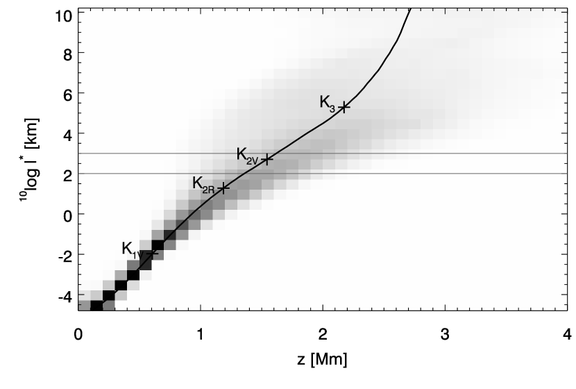
Figure 8.— Distribution of photon mean free paths as function of height in the 3DMHD model atmosphere at Mg II k line center. The median of the mean free path as function of height is shown in solid black. The crosses indicate the average $\tau=1$ heights at wavelengths for various spectral features in the average profile: the minimum on the blue side of the central emission peaks (k_1V), the red (k_2R) and blue (k_2V) emission peaks and the line-center depression (k₃). The grey lines indicate a free path of 100 km and 1000 km to guide the eye.

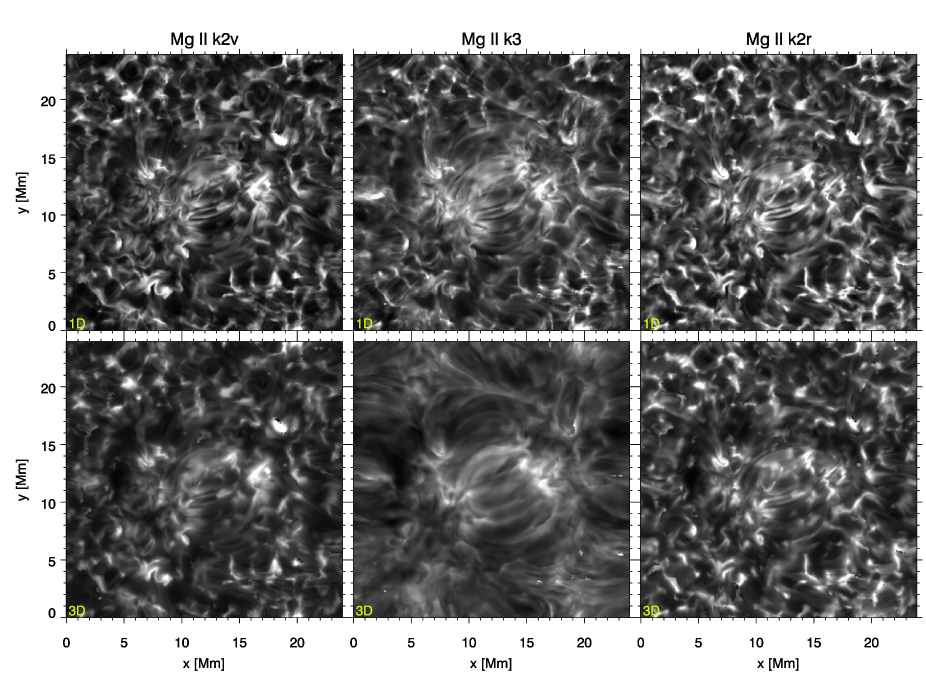
Figure 9.— Comparison of the vertically emergent intensity in the Mg II k line core between a 1D (top row) and 3D (bottom row) computation, performed assuming CRD. The columns show the intensity for various spectral features indicated above the top panels. The top and bottom panels in each column have the same brightness scale so the 1D and 3D intensity can be compared directly.

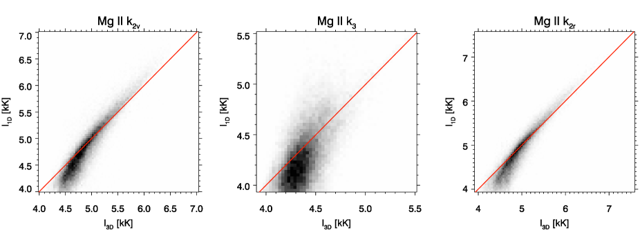
Figure 10.— Joint probability density functions of the vertically emergent intensity computed in 3D and in 1D. Left: k_2V; middle: k₃; right: k_2R. The red line is the line $I_{\mathrm{1D}}=I_{\mathrm{3D}}$.

The Mg II  h&k lines are strongly scattering as illustrated by Fig. 6, which shows that the probability for radiative de-excitation from the upper levels is 4 orders of magnitude larger than the probability for collisional de-excitation. This means that the source function is largely set by the radiation field, which in turn depends on the atmospheric structure. If the typical effective photon mean free path is comparable to or larger than the scale of the horizontal inhomogeneities in the atmosphere then effects of horizontal radiation transport are important. Typically, this leads to a smoothing of the radiation field and a corresponding smoothing of the source function.

We estimate the 3D effects by using the expression for an infinitely sharp-lined, two-level atom with isotropic scattering. In that case the effective photon mean free path can be expressed in terms of the opacity $\alpha$ and the photon destruction probability $\epsilon$:

$$l^{\star}=\frac{1}{\alpha_{\nu}\sqrt{\epsilon}}.$$ (3)

The photon destruction probability is given by

$$\epsilon=\frac{C_{{\rm u}{\rm l}}}{C_{{\rm u}{\rm l}}+A_{{\rm u}{\rm l}}+B_{{\rm u}{\rm l}}B_{\nu}},$$ (4)

with $C_{{\rm u}{\rm l}}$, $A_{{\rm u}{\rm l}}$ and $B_{{\rm u}{\rm l}}$ the coefficient for collisional de-excitation, the Einstein coefficients for spontaneous de-excitation and induced de-excitation, and $B_{\nu}$ the Planck function.

We computed $l^{\star}$ for the Mg II k line in the 3DMHD atmosphere, from a 3D non-LTE CRD computation with Multi3d  taking as opacity the line-center absorption coefficient for an outgoing vertical ray. In Fig. 8 we compare it with the average height of formation of the k₁, k_2R, k_2V and k₃ spectral features. Based on this rough estimate we expect that the k₁ and k_2R intensities are not affected by 3D effects. The k_2V peak is marginally affected at the horizontal resolution of the radiative transfer computation (96 km, compared to a median photon mean free path of $\approx 300$ km), while k₃ is strongly affected.

We confirm this in Figure 9, where we compare the vertically emergent intensity in k_2V, k₃ and k_2R computed in 3D and 1D, but assuming CRD. For each pixel in the image we determined the wavelength of the spectral features using an automated algorithm. Because of the very complex, multiple-peaked profiles, this algorithm does not correctly identify the spectral locations of the features for all pixels. These pixel locations show up as noise (dark pixels in k_2V and k_2R, bright pixels in k₃).

The k_2V and k_2R spectral features are weakly affected by 3D effects. Typically, the dark areas are brighter in 3D than in 1D, and the 3D image is slightly fuzzier. The k₃ image is strongly affected by 3D effects. The 3D image is much fuzzier, and there is a much more pronounced fibril structure than in 1D. In 1D there are only fibrils visible in the central region, where the chromospheric magnetic field is strongest. Elsewhere the 1D image shows shock waves with a structure very similar to what is seen in the k_2Vimage.

The same information is shown as the joint probability density function (JPDF) of the 3D and 1D intensities in Figure 10. It confirms the impression from the images in Figure 9: 3D effects are strong for k₃, and much weaker for k_2Vand k_2R.

For the two emission peaks the largest 3D effects occur at low intensities, where the 3D intensity is larger than the 1D intensity. This is caused by the sideways illumination of cool parts of the atmosphere by hotter neighboring locations. This illumination leads to a higher angle-averaged radiation field in 3D, and thus to a higher source function and emergent intensity. The reverse happens for locations with a high k_2Vand k_2R intensity; there the 3D radiation field is lower than in 1D owing to the lateral averaging. The k_2R peak intensity is slightly less influenced by 3D effects than k_2V, in agreement with the lower formation height of k_2R(see Figure 8).

The k₃ intensity minimum shows only a weak correlation between 1D and 3D intensity, as expected based on the different appearance of the 1D and 3D images in Figure 9.

We performed the same analysis for the h line and reached the same conclusions.

11. Effect of partial redistribution

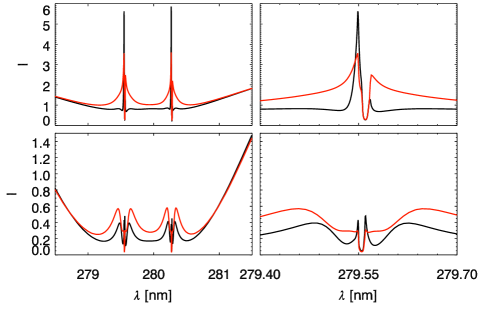
Figure 11.— Comparison of the emergent Mg II  h&k line profiles in two locations of the 3DMHD atmosphere (top and bottom row). The left-hand column shows both h&k lines, the right-hand column shows a zoom of the line core of the k line. The black curve is the PRD profile, the red curve the CRD profile. The intensity is given in units of 10^-9 J m^-2 s^-1 Hz^-1 sr^-1.

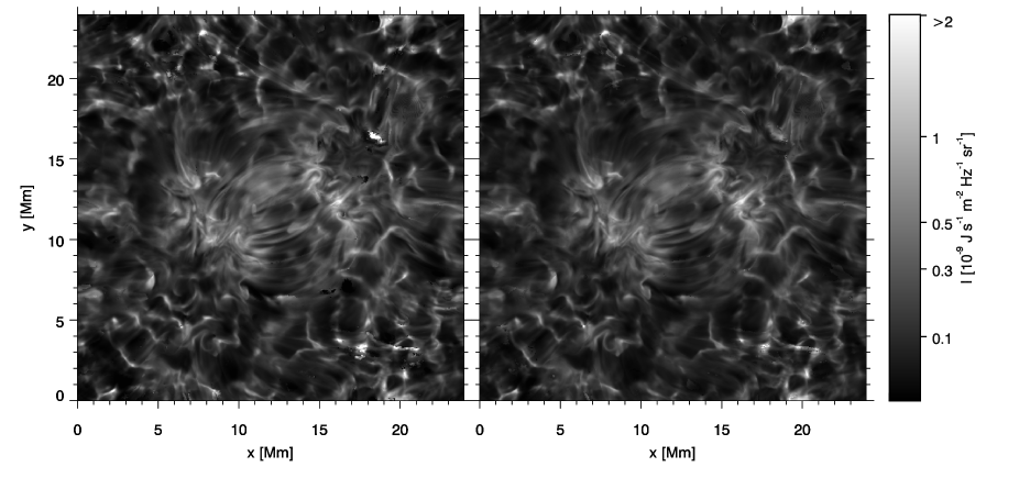
Figure 12.— Comparison of the k₃ intensity computed in 1D with PRD (left-hand panel) and CRD (right-hand panel). Both images have the same brightness scale, given on the right. Columns where the wavelength of k₃ is misidentified appear as white pixels.

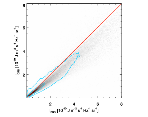
Figure 13.— Joint probability density function of the intensity in Mg II k₃ computed in PRD (horizontal axis) and CRD (vertical axis). Darker color indicates a higher number of pixels in the bin. The image has been clipped and scaled to bring out the distribution at high intensities. The red line indicates $I_{\mathrm{PRD}}=I_{\mathrm{CRD}}$. The inner blue contour encloses 50% of all pixels, the outer blue contour encloses 90% of all pixels.

We now turn our attention to the effect of PRD on the emergent line profiles. The Mg II  h&k lines are strongly affected by the effect of partial redistribution. Owing to the low particle density in the chromosphere, the average time between collisions is large compared to the lifetime of a Mg II ion in the upper levels of the lines. Therefore, the frequency of the absorbed and emitted photon in a scattering process are correlated and the assumption of complete redistribution is invalid. We demonstrate this effect in Fig. 11, which displays a comparison of vertically emergent line profiles computed with RH in PRD and CRD for two different columns in the 3DMHD atmosphere. These computations were done assuming the 1D plane-parallel approximation.

Inclusion of PRD has the strongest effect in the inner wing of the line profile. Typically the PRD computations yield a lower inner-wing intensity (around the k₁ minima) and a higher intensity in the emission peaks (k_2V and k_2R). The intensity in the k₃ minimum is only weakly influenced by PRD effects. Images of the k₃ intensity computed in PRD and CRD from the 3DMHD atmosphere appear nearly identical as shown in Fig. 12.

A more quantitative comparison is given in Fig. 13, which shows the JPDF of the intensity in Mg II k₃ computed in PRD and CRD. At low intensities there is a very tight correlation between the PRD and CRD computations, at higher intensities the correlation becomes somewhat weaker and the PRD intensity tends to be higher than the CRD intensity. In general, assuming CRD for the k₃ minimum is a very good approximation.

12. Discussion and conclusions

We studied the basic formation properties of the Mg II  h&k lines in models of the solar atmosphere.

We first investigated the time dependent, non-equilibrium ionization balance of Mg II/Mg III and found that whenever the temperature is high enough to give a significant fraction of Mg III, the relaxation time is short. We therefore conclude that statistical equilbrium is a good approximation for the formation of the Mg II  h&k lines.

We then investigated the influence of Mg I on the line formation and found that treating neutral magnesium in LTE as a source of background opacity leads to lower intensity in the outer line wings. The h&k line cores are unaffected. If one is interested in the outer wing intensities, one should include Mg I in the non-LTE model atom. We used a model with 65 bound levels of Mg I. It is possible that a smaller number of Mg I levels is sufficient to model the effect on the h&k lines. If so, this would reduce the required computational effort significantly.

We then constructed a minimal model atom that models the h&k lines. This model atom contains four bound levels and a continuum. The bound levels are the Mg II ground state, the 2p⁶3p doublet which are the upper levels of the lines, and a higher-lying artificial level that is required to correctly recover the Mg II–Mg III ionization balance. This aritificial level acts as a target level for recombination of Mg III. Omitting this level leads to an incorrect ionization balance in the upper chromosphere and too low emission peaks.

Our investigation of the difference between the h line and the k line confirm the conjecture by Linsky & Avrett (1970), that the stronger emission in the k line is because the k line has twice the opacity of the h line. This larger opacity causes a larger formation height, and a stronger coupling of the source function to the gas temperature at the locations in the atmosphere where the emission peaks form.

The Mg II  h&k lines are scattering lines, and the emergent intensity is influenced by 3D effects in the line core. The intensity in the emission peaks are only mildly affected: in 3D contrast is decreased compared to 1D computations, but the overall appearance of the images computed from the 3DMHD model remains the same. The k₃ and h₃ intensity minima are strongly affected by 3D effects: 3D images are fuzzier and show long extended fibrils. Intensity minimum images computed in 1D show only a very weak imprint of fibrils and instead exhibit a shock wave pattern similar to images of the intensity in the emission peaks.

The assumption of complete redistribution is not valid for Mg II  h&k. The line profiles must be computed assuming partial redistribution, otherwise the line-wing intensity up to and including the emission peaks will be wrong. However, the intensity in the k₃ and h₃ minima computed in CRD is very similar to the correct intensity computed in PRD.

Based on this analysis we can now answer the question how best to model the Mg II  h&k lines in time-series of snapshots from large 3D radiation-MHD models:

The current state-of-the-art in unpolarized non-LTE radiative transfer modeling allows for quick computation of line profiles including PRD treating each column in the snapshot as an independent 1D plane-parallel atmosphere. Radiative transfer computations taking the full 3D structure into account are also possible, but only assuming CRD. Non-LTE computations including both PRD and 3D simultaneously are currently not possible: inclusion of PRD in the non-LTE computations occasionally leads to instabilities in the Lambda-iteration. In 1D this would only lead to a non-converged column, but in 3D the whole computation would fail. This is a problem for modeling the h&k lines, which are influenced both by 3D and PRD effects. Our results show, however, that by combining 1D PRD and 3D CRD computations one can capture the essentials of the true profile. The profile up to and including the emission peaks are well approximated by 1D PRD. The central depression can be modelled reasonably well with 3D CRD computations. We stress that a 1D CRD approach is not realistic and should not be used.

While this combined approach is not truly satisfactory, it nevertheless opens up the possibility of modeling the Mg II  h&k lines with enough realism to study their formation in 3D numerical models of the solar atmosphere and determine their potential as atmospheric diagnostics. We report on the results of such a study in paper II of this series.

References

- Abia & Mashonkina (2004) Abia, C. & Mashonkina, L. 2004, MNRAS, 350, 1127
- Allen & McAllister (1978) Allen, M. S. & McAllister, H. C. 1978, Sol. Phys., 60, 251
- Anstee & O’Mara (1995) Anstee, S. D. & O’Mara, B. J. 1995, MNRAS, 276, 859
- Arnaud & Rothenflug (1985) Arnaud, M. & Rothenflug, R. 1985, A&AS, 60, 425
- Artzner et al. (1978) Artzner, G., Vial, J. C., Lemaire, P., Gouttebroze, P., & Leibacher, J. 1978, ApJ, 224, L83
- Asplund et al. (2009) Asplund, M., Grevesse, N., Sauval, A. J., & Scott, P. 2009, ARA&A, 47, 481
- Barklem & O’Mara (1998) Barklem, P. S. & O’Mara, B. J. 1998, MNRAS, 300, 863
- Bonnet et al. (1978) Bonnet, R. M., Lemaire, P., Vial, J. C., et al. 1978, ApJ, 221, 1032
- Burgess & Chidichimo (1983) Burgess, A. & Chidichimo, M. C. 1983, MNRAS, 203, 1269
- Carlsson & Leenaarts (2012) Carlsson, M. & Leenaarts, J. 2012, A&A, 539, A39
- Carlsson et al. (1992) Carlsson, M., Rutten, R. J., & Shchukina, N. G. 1992, A&A, 253, 567
- Carlsson & Stein (1992) Carlsson, M. & Stein, R. F. 1992, ApJ, 397, L59
- Carlsson & Stein (1997) Carlsson, M. & Stein, R. F. 1997, ApJ, 481, 500
- Carlsson & Stein (2002) Carlsson, M. & Stein, R. F. 2002, ApJ, 572, 626
- Chang et al. (1991) Chang, E. S., Avrett, E. H., Noyes, R. W., Loeser, R., & Mauas, P. J. 1991, ApJ, 379, L79
- Cunto et al. (1993) Cunto, W., Mendoza, C., Ochsenbein, F., & Zeippen, C. J. 1993, A&A, 275, L5
- Dorfi & Drury (1987) Dorfi, E. A. & Drury, L. O. 1987, Journal of Computational Physics, 69, 175
- Fontenla et al. (1991) Fontenla, J. M., Avrett, E. H., & Loeser, R. 1991, ApJ, 377, 712
- Fontenla et al. (1993) Fontenla, J. M., Avrett, E. H., & Loeser, R. 1993, ApJ, 406, 319
- Gouttebroze (1989) Gouttebroze, P. 1989, ApJ, 337, 536
- Gudiksen et al. (2011) Gudiksen, B. V., Carlsson, M., Hansteen, V. H., et al. 2011, A&A, 531, A154
- Hayek et al. (2010) Hayek, W., Asplund, M., Carlsson, M., et al. 2010, A&A, 517, A49
- Kneer et al. (1981) Kneer, F., Mattig, W., Scharmer, G., et al. 1981, Sol. Phys., 69, 289
- Kohl & Parkinson (1976) Kohl, J. L. & Parkinson, W. H. 1976, ApJ, 205, 599
- Leenaarts & Carlsson (2009) Leenaarts, J. & Carlsson, M. 2009, in Astronomical Society of the Pacific Conference Series, Vol. 415, Astronomical Society of the Pacific Conference Series, ed. B. Lites, M. Cheung, T. Magara, J. Mariska, & K. Reeves, 87
- Leenaarts et al. (2011) Leenaarts, J., Carlsson, M., Hansteen, V., & Gudiksen, B. V. 2011, A&A, 530, A124
- Leenaarts et al. (2007) Leenaarts, J., Carlsson, M., Hansteen, V., & Rutten, R. J. 2007, A&A, 473, 625
- Leenaarts et al. (2012a) Leenaarts, J., Carlsson, M., & Rouppe van der Voort, L. 2012a, ApJ, 749, 136
- Leenaarts et al. (2012b) Leenaarts, J., Pereira, T., & Uitenbroek, H. 2012b, A&A, 543, A109
- Lemaire & Samain (1989) Lemaire, P. & Samain, D. 1989, in High spatial resolution solar observations, 551
- Linsky (1970) Linsky, J. L. 1970, Sol. Phys., 11, 355
- Linsky & Avrett (1970) Linsky, J. L. & Avrett, E. H. 1970, PASP, 82, 169
- Mihalas (1978) Mihalas, D. 1978, Stellar atmospheres /2nd edition/ (San Francisco, W. H. Freeman and Co., 1978. 650 p.)
- Milkey & Mihalas (1974) Milkey, R. W. & Mihalas, D. 1974, ApJ, 192, 769
- Monteiro et al. (1988) Monteiro, T. S., Danby, G., Cooper, I. L., Dickinson, A. S., & Lewis, E. L. 1988, Journal of Physics B Atomic Molecular Physics, 21, 4165
- Morrill et al. (2001) Morrill, J. S., Dere, K. P., & Korendyke, C. M. 2001, ApJ, 557, 854
- Morrill & Korendyke (2008) Morrill, J. S. & Korendyke, C. M. 2008, ApJ, 687, 646
- Nordlund (1982) Nordlund, A. 1982, A&A, 107, 1
- Ralchenko et al. (2011) Ralchenko, Y., Kramida, A., Reader, J., & NIST ASD Team. 2011, in http://physics.nist.gov/asd
- Rezaei et al. (2008) Rezaei, R., Bruls, J. H. M. J., Schmidt, W., et al. 2008, A&A, 484, 503
- Rutten (2003) Rutten, R. J. 2003, Radiative Transfer in Stellar Atmospheres, ed. Rutten, R. J.
- Shull & van Steenberg (1982) Shull, J. M. & van Steenberg, M. 1982, ApJS, 49, 351
- Sigut & Pradhan (1995) Sigut, T. A. A. & Pradhan, A. K. 1995, Journal of Physics B Atomic Molecular Physics, 28, 4879
- Skartlien (2000) Skartlien, R. 2000, ApJ, 536, 465
- Staath & Lemaire (1995) Staath, E. & Lemaire, P. 1995, A&A, 295, 517
- Tousey (1967) Tousey, R. 1967, ApJ, 149, 239
- Uitenbroek (1997) Uitenbroek, H. 1997, Sol. Phys., 172, 109
- Uitenbroek (2001) Uitenbroek, H. 2001, ApJ, 557, 389
- Uitenbroek & Briand (1995) Uitenbroek, H. & Briand, C. 1995, ApJ, 447, 453
- Vial (1984) Vial, J.-C. 1984, L’Astronomie, 98, 211
- Vial et al. (1979) Vial, J. C., Gouttebroze, P., Artzner, G., & Lemaire, P. 1979, Sol. Phys., 61, 39
- Vial et al. (1981) Vial, J. C., Salm-Platzer, J., & Martres, M. J. 1981, Sol. Phys., 70, 325
- West et al. (2011) West, E., Cirtain, J., Kobayashi, K., et al. 2011, in Society of Photo-Optical Instrumentation Engineers (SPIE) Conference Series, Vol. 8160, Society of Photo-Optical Instrumentation Engineers (SPIE) Conference Series
- Woodgate et al. (1980) Woodgate, B. E., Brandt, J. C., Kalet, M. W., et al. 1980, Sol. Phys., 65, 73
- Zhao et al. (1998) Zhao, G., Butler, K., & Gehren, T. 1998, A&A, 333, 219