Dephasing-assisted parameter estimation in the presence of dynamical decoupling

Abstract

We study the dephasing-assisted precision of parameter estimation (PPE) enhancement in atom interferometer under dynamical decoupling (DD) pulses. Through calculating spin squeezing (SS) and quantum Fisher information (QFI), we find that dephasing noise can improve PPE by inducing SS, and the DD pulses can maximize the improvement. It is indicated that in the presence of DD pulses, the dephasing-induced SS can reach the limit of “one-axis twisting” model, $\xi^{2}\simeq N^{-2/3}$ with $\xi^{2}$ being the SS parameter and $N$ the number of atoms. In particular, we find that the DD pulses can amplify the dephasing-induced QFI by a factor of $\simeq N/2$ compared with the noise-free case, which means that under the control of DD pulses, the dephasing noise can enhance the PPE to the scale of $\sqrt{2}/N$, the same order of magnitude of Heisenberg limit ($1/N$).

I Introduction

Atom interferometry has attracted much attention because of its potential applications in quantum metrology gus ; fix ; cro ; gros ; bar ; rie ; gro ; mj . Atomic Bose-Einstein condensates (BECs) due to their unique coherence properties and the possibility to yield controlled nonlinearity are viewed as the ideal sources for an atom interferometer bou ; kas . The nonlinearity of BECs caused by interatomic interactions can create squeezed states ore ; wine ; ueda ; jgr ; pezz ; YCL , which can improve the precision of parameter estimation (PPE).

The ability of BECs to create highly squeezed states and serve as nonlinear interferometers, whose precision exceeds the standard quantum limit (SQL) achieved with coherent spin states (CSS), has been demonstrated in two recent experiments gros ; rie . However, the atom-atom nonlinear interaction strength caused by s-wave scattering is usually very small when the modes of the BEC have a spatial overlap mj ; gros ; rie . Such nonlinearity enhancement currently resorts to the use of Feshbach resonances gros or spatially separating the components of BEC rie , but the price of these methods is significantly increased atom losses, limiting the achievable squeezing. In Ref. bar , the authors proposed an approach to drastically enhance the nonlinear dynamics of the BEC based on collisions of the BEC with a thermal reservoir and attained a strongly squeezing. This enhanced squeezing stems from the decoherence noise which implies that the reservoir noise can also be regarded as a resource to improve the parameter estimation sensitivity. However, it is well known that the decoherence typically play a coherence-destructive role which is one of the main obstacles to produce certain spin-squeezed states (SSS). Much research showed that the decoherence may prevent the production of certain SSS and limit the precision of quantum metrology sim ; and ; sto ; li ; sin ; wata ; wang . Thus, it is important to suppress the coherence-destructive role but at the same time maintain the decoherence-induced nonlinearity interaction if one wants to obtain a strong squeezing and improve PPE.

Dynamical decoupling (DD) technique vio ; kho ; gord ; uhr ; yang ; du ; DJF ; GJB ; pan ; tan , which has been widely employed in the area of quantum information, provides an active way to fight against decoherence. Recently, this technique has also been introduced into the field of magnetometers to improve the sensitivity of oscillating magnetic fields based on nitrogen-vacancy centers tay ; lan ; G.G ; hall . Combining the DD technique with quantum metrology can preserve PPE in noisy system by suppressing the decoherence effect tan . Thus a natural question rises, is it possible to realize decoherence-enhanced PPE under the DD pulses?

In this paper, we give a positive answer to the above question by investigating the influence of the DD pulses on the dephasing-induced SS and dephasing-amplified quantum Fisher information (QFI) pezz ; brau ; hels ; giova ; sunz ; ferr ; maj ; huang , which are two important quantities relevant in parameter estimationpezz ; ferr . We compare the effects of two different DD pulse sequence: periodic DD (PDD) sequence vio ; kho and Uhrig DD (UDD) sequence uhr ; yang . Our finding shows that both these sequences can effectively suppress the coherence-destructive role and maintain the decoherence-induced nonlinearity interaction. It is also found that the UDD sequence can work more efficiently, which can enhance the decoherence-induced SS to the limit of $\xi^{2}\simeq N^{-2/3}$ ueda ; jgr more easily, where $\xi^{2}$ is the SS parameter and $N$ is the number of atoms. In particular, we find that it is possible for the UDD sequence to amplify the QFI by a factor of $\simeq N/2$ compared with the initial CSS in the case of pure dephasing. It means that the dephasing-assisted sensitivity of the estimated parameter can be enhanced from the SQL $1/\sqrt{N}$ to $\sqrt{2}/N$, which approaches nearly Heisenberg-limited precision $(1/N)$ gio ; hue .

This paper is organized as follows. In Sec. II, we introduce our physical model and Hamiltonian in the presence of control pulses. We then investigate the dynamical evolution of the BEC system in the dephasing environment with two different DD-pulse sequences. It is indicated that the DD-pulse sequences can effectively suppress the coherence-destructive role while maintaining the decoherence-induced nonlinearity interaction. In Sec. III, we study the effects of DD pulses on enhancing the dephasing-induced spin squeezing. We show that the magnitude of SS in the limit of $\xi^{2}\simeq N^{-2/3}$ can be induced by the dephasing noise in the presence of DD pulses. Section IV discusses the dephasing-assisted QFI amplification under the DD pulses. It is found that the DD pulses can greatly amplify the QFI and enhance the PPE to the scale of Heisenberg limit. Finally, we conclude this work in Sec. V.

II Dephasing in two-component Bose-Einstein condensate system with DD pulse sequences

In this section, we consider a two-component BEC system confined in a harmonic potential, which suffers from dephasing noise.

II.1 Model and Hamiltonian

The total Hamiltonian is supposed to be

$$H=\lambda\epsilon(s)J_{z}+\chi J_{z}^{2}+\sum_{k}\omega_{k}b_{k}^{{\dagger}}b_{k}+\epsilon(s)J_{z}\sum_{k}g_{k}\left(b_{k}^{{\dagger}}+b_{k}\right),$$ (1)

which is the “one-axis twisting” (OAT) model in the presence of environment noise as well as DD control. Angular momentum operators $J_{+}=(J_{-})^{{\dagger}}=b^{{\dagger}}a$ and $J_{z}=(b^{{\dagger}}b-a^{{\dagger}}a)/2$ satisfy SU(2) algebra, with $a$ and $b$ being the annihilation operators for two internal hyperfine states $\left|a\right\rangle$ and $\left|b\right\rangle$ of the condensed atoms. The nonlinear interaction strengthen $\chi$ can be controlled by using a Feshbach resonancegros . $\epsilon(s)$ is the time-dependent modulation filed induced by $n$ DD $\pi$ pulses gord , which reverse the sign of $J_{z}$ at time $t_{j}$, and is given by

$$\epsilon(s)=\sum_{j=0}^{n}(-1)^{j}\theta(s-t_{j})\theta(t_{j+1}-s),$$ (2)

with $s\in[0,t].$ Here the total time interval $0\rightarrow t$ is split into $n+1$ small intervals $t_{j}$ which satisfy $t_{0}=0$ and $t_{n+1}=t.$ In the above equation the step function $\theta(x)$ is equal to 1 if $x>0$ and 0 if $x<0$.

In the interaction picture with respect to the reservoir operator $\sum_{k}\omega_{k}b_{k}^{{\dagger}}b_{k}$, the time evolution operator can be obtained by using Magnus expansion bar ; bla

$$U(t)=\mathrm{T}_{+}\exp\left[-i\int_{0}^{t}H_{I}(t^{\prime})dt^{\prime}\right]=\exp\left[iJ_{z}^{2}\Omega(t)\right]V(t),$$ (3)

where the noise-induced nonlinear interaction strength can be recasted as

$$\Omega(t)=\sum_{k}g_{k}^{2}\int_{0}^{t}ds\int_{0}^{s}ds^{\prime}\epsilon(s)\epsilon(s^{\prime})\sin\omega_{k}(s-s^{\prime}).$$ (4)

In Eq. (3), the unitary operator $V(t)$ is defined by

$$V(t)=e^{-i\int_{0}^{t}[\lambda\epsilon(s)J_{z}+\chi J_{z}^{2}]ds}e^{J_{z}\sum_{k}(\alpha_{k}b_{k}^{{\dagger}}-\alpha_{k}^{\ast}b_{k})},$$ (5)

with the amplitudes $\alpha_{k}=-ig_{k}\int_{0}^{t}e^{i\omega_{k}s}\epsilon(s)ds$. Furthermore, according to the experiment gros , the nonlinear interaction strength $\chi$ is very small, $\chi\simeq 0$, if without the Feshbach resonance. Thus we further have

$$U(t)=e^{-i\phi}\exp[i\Omega(t)J_{z}^{2}]\exp\left[J_{z}\sum_{k}(\alpha_{k}b_{k}^{{\dagger}}-\alpha_{k}^{\ast}b_{k})\right],$$ (6)

with $\phi=J_{z}\int_{0}^{t}\lambda\epsilon(s)ds$  which can be removed when appropriate DD pulses sequences are applied, such as the UDD pulses sequence and the odd number of PDD pulses sequence.

II.2 System dynamical evolution under DD-pulse sequences

In what follows, we investigate the dynamical evolution of the BEC system in the dephasing environment with DD-pulse sequences. Let us assume that the initial state of the total system is given by

$$\rho(0)=\left|\Psi(0)\right\rangle\left\langle\Psi(0)\right|\otimes\rho_{B},$$ (7)

where

$$\left|\Psi(0)\right\rangle=\sum_{m}c_{m}(0)\left|j,m\right\rangle$$

is the CSS, with the probability amplitudes $c_{m}=2^{-j}\left(C_{2j}^{j+m}\right)^{1/2}$ and   total spin $j=N/2$ for a system consisting of $N$ atoms. Such a state is the optimal initial state to obtain the strongest squeezingueda ; jgr . In Eq. (7), $\rho_{B}$ is the thermal equilibrium state of reservoir, defined by

$$\rho_{B}=\Pi_{k}[1-\exp(-\beta\omega_{k})]\exp(-\beta\omega_{k}b_{k}^{{\dagger}}b_{k}),$$

with $\beta$ the inverse temperature ($\beta=1/T$).

Based on Eq. (5), the matrix elements of the system’s density matrix can be determined from the relation

$$\rho_{jm,jn}(t) = \mathrm{Tr}_{B}\left[\left\langle j,m\right|U(t)\rho(0)U^{-1}(t)\left|j,n\right\rangle\right]$$

$$= e^{-i(\phi_{m}-\phi_{n})}e^{i(m^{2}-n^{2})\Omega(t)}\exp\left[-(m-n)^{2}R(t)\right]\rho_{jm,jn}(0).$$

In the above equation the decoherence function (see Appendix A for details)

$$R(t)=\int_{0}^{\infty}d\omega\mathrm{F}(\omega,t)G\text{ }(\omega)$$ (9)

is the overlap integral of the temperature-dependent interacting spectrum

$$G(\omega)=J(\omega)[2n(\omega)+1]=J(\omega)\coth(\beta\omega/2),$$

where $n(\omega)=[\exp(\beta\omega)-1]^{-1}$ is the bosonic distribution function of the heat reservoir, $J(\omega)$ is the spectral density. The filter function of an $n$-pulse sequence

$$\mathrm{F}_{n}(\omega,t) \equiv \frac{\left|\epsilon(\omega)\right|^{2}}{2}=\frac{1}{2}\left|\int_{0}^{t}e^{i\omega s}\epsilon(s)ds\right|^{2}$$

$$= \frac{1}{2\omega^{2}}\left|1+(-1)^{n+1}e^{i\omega t}+2\sum_{j=1}^{n}(-1)^{j}e^{i\omega t_{j}}\right|^{\begin{subarray}{c}2\end{subarray}}.$$

Substituting the spectral density $J(\omega)$ into Eq. (4), the noise-induced nonlinear term in Eq. (8) can be recasted as (see Appendix B )

$$\Omega(t)=\int_{0}^{\infty}d\omega J(\omega)f_{n}(\omega,t),$$ (10)

with

$$f_{n}(\omega,t) = \mathrm{\vartheta}(\omega,t)+\mathrm{\mu}(\omega,t)+t/\omega,$$

$$\mathrm{\vartheta}(\omega,t) = \frac{1}{\omega^{2}}\left[(-1)^{n+1}\sin(\omega t)-2\sum_{m=1}^{n}(-1)^{m}\sin(\omega t_{m})\right],$$

$$\mathrm{\mu}(\omega,t) = \frac{2}{\omega^{2}}\left\{\sum_{m=1}^{n}\sum_{j=1}^{m}(-1)^{m+j}\left(\sin[\omega(t_{m}-t_{j})]\right.\right.$$ (11)

$$-\left.\left.\sin[\omega(t_{m+1}-t_{j})]\right)\right\}.$$

Note that the result attained in the above equation is more complex than that in Ref. uhr for single-qubit DD.

For an ohmic bath in the continuum limit,

$$J(\omega)=\alpha\omega e^{-\omega/\omega_{c}}$$

with $\alpha$ the coupling strength between the system and the reservoir and $\omega_{c}$ the cutoff frequency, we find, in the absence of control $(n=0)$ lmk ; hp

$$R(t) = \alpha\int_{0}^{\infty}d\omega\omega e^{-\omega/\omega_{c}}\coth(\beta\omega/2)\frac{1-\cos(\omega t)}{\omega^{2}},$$ (12)

$$\Omega(t) = \alpha\int_{0}^{\infty}d\omega\omega e^{-\omega/\omega_{c}}\frac{\omega t-\sin(\omega t)}{\omega^{2}}$$ (13)

$$= \alpha[\omega_{c}t-\arctan(\omega_{c}t)],$$

where the decoherence function $R(t)$ can be further reduced as

$$R(t)=\alpha\left\{\frac{1}{2}\ln(1+\omega_{c}^{2}t^{2})+\ln\left[\frac{\beta}{\pi t}\sinh({\pi t}/{\beta})\right]\right\}$$

in the low temperature case ($\beta\omega_{c}\ll 1$).

If we consider the PDD sequence, in which sequence the $\pi$-pulse is applied at equidistant intervals

$$t_{j}^{\mathrm{PDD}}=jt/(n+1),$$

then the modulation spectrums $\mathrm{F}_{n}(\omega,t)$ and $f_{n}(\omega,t)$ in Eqs. (9) and (10) can be given by uhr

$$\mathrm{F}_{n}^{\mathrm{PDD}}(\omega,t) = \tan^{2}[\omega t/(2n+2)][1+(-1)^{n}\cos(\omega t)]/\omega^{2},$$

$$f_{n}^{\mathrm{PDD}}(\omega,t) = \frac{2(-1)^{n+1}\sin(\omega t)+\omega t}{\omega^{2}}$$ (14)

$$+2\tan\left(\frac{\omega t}{2n+2}\right)\frac{(-1)^{n}\cos(\omega t)-n}{\omega^{2}}$$

$$+\tan^{2}\left(\frac{\omega t}{2n+2}\right)\frac{(-1)^{n}\sin(\omega t)}{\omega^{2}}.$$

Whereas for the UDD sequence uhr

$$t_{j}^{\mathrm{UDD}}=t\sin^{2}\left[{j\pi}/{(2n+2)}\right],$$

the filter function is

$$\mathrm{F}_{n}^{\mathrm{UDD}}(\omega,t)\approx 8(n+1)^{2}J_{n+1}^{2}(\omega t/2)/\omega^{2},$$ (15)

where $J_{n}(x)$ is the Bessel function. The function $f_{n}^{\mathrm{UDD}}(\omega,t)$ can be got by inserting $t_{j}^{\mathrm{UDD}}$ into Eq. (II.2). The form of the expression is very complex, and we do not give it here.

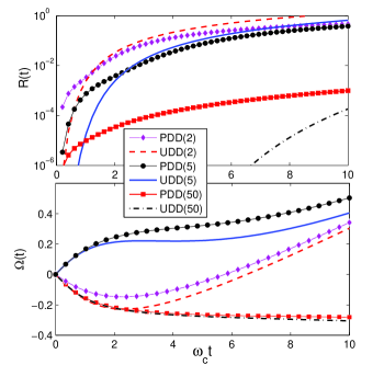
Figure 1: (Color online) Comparison of dynamical behaviors of functions $R(t)$ and $\Omega(t)$ under two different DD-pulse sequences. Relevant parameters are chosen as coupling strength $\alpha=0.1$ and temperature $T=\omega_{c}$.

Although both the functions of $R(t)$ and $\Omega(t)$ stem from environment noise, they play different roles. In other words, $\Omega(t)$ can induce the quantum correlation in the system, while $R(t)$ destroys it. These results imply that if one wants to make full use of the advantage of environment noise to generate the desired quantum correlation, the coherence-destructive process must be suppressed. Fortunately, according to Eqs. (9)-(15) as well as Fig. 1, it is found that the DD-pulse can effectively average the decoherence function $R(t)$ nearly to zero, but do not remove the noise-induced nonlinear term $\Omega(t)$.

In the discussion below, we will investigate how to attain the best squeezing and QFI, which are two quantities relevant in interferometry, in the presence of dephasing by using of DD-pulse sequences.

III Dephasing-induced spin squeezing in the present of DD-pulses sequences

In this section, we shall evaluate the magnitude of the dephasing-induced SS as well as study how to improve it by employing the DD schemes as considered above. To quantify the degree of SS, we introduce the SS parameter given by Kitagawa and Ueda ueda

$$\xi^{2}=\frac{2(\Delta J_{{\vec{n}}_{\bot}})_{\min}^{2}}{j},$$ (16)

where the minimization in the equation is over all directions denoted by $\vec{n}_{\bot}$, perpendicular to the mean spin direction.

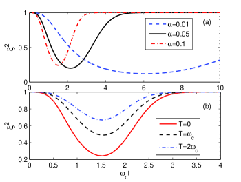
Figure 2: (Color online) Dephasing-induced spin squeezing in the absence of control pulses ($n=0$). (a) Varying with different coupling strengthen $\alpha$ with fixed $T=0$. (b) Varying with different values of temperature with fixed $\alpha=0.1$. The number of atoms is $N=200$.

With the use of Eq. (II.2), we can obtain the degree of dephasing-induced SS for the initial state given in Eq. (7) ueda ; jgr in the case of pure dephasing noise

$$\xi^{2}=1+\frac{2j-1}{4}(A-\sqrt{A^{2}+B^{2}}),$$ (17)

in the optimally squeezed direction $\psi_{\text{opt}}=[\pi+\tan^{-1}({B}/{A})]/2$, where

$$A = 1-\cos^{2j-2}[2\Omega(t)]e^{-4R(t)},$$

$$B = -4\sin[\Omega(t)]\cos^{2j-2}[\Omega(t)]e^{-R(t)}.$$ (18)

Compared with Refs. ueda ; jgr , the controllable decoherence function $R(t)$ is introduced and the scaled time $\chi t$ is replaced by $\Omega(t)$ in the above equations. From the above equations, we can clearly find again that dephasing noise plays two roles: on one hand, it can generate the SS by inducing the nonlinear interaction $\Omega(t)$; on the other hand, it degrade the degree of SS via the decoherence function $R(t)$. And from the Eqs. (9), (14) and (15), it is found that if $t/(n+1)\rightarrow 0$, we have $R(t)\rightarrow 0$, then the coherence-destructive effect is suppressed. Therefore, in the short-time limit ($\Omega(t)\ll 1$) and the large particle number limit ($j\gg 1$), the best squeezing can be approximated as

$$\xi_{\min}^{2}\simeq\frac{3}{4j}(\frac{2j}{3})^{1/3}\simeq N^{-2/3},$$ (19)

which is the well known result appeared in Ref. ueda ; jgr for an ideal noise-free case.

In Fig. 2, we plot the dynamics of dephasing-induced SS in the absence of control pulses. From Fig. 2 we can find that the decoherence not only generate SS but also prevent the production of certain SS; and the stronger coupling strength [Fig. 1(a)] or the higher the temperature [Fig. 1(b)] is, the weaker the squeezing is attained. In all these cases the best squeezing given in Eq. (19) cannot be reached.

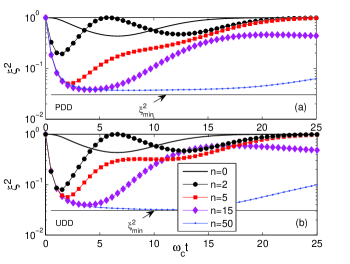
Figure 3: (Color online) Spin squeezing $\xi^{2}$ with respect to scaled time $\omega_{c}t$ for (a) PDD sequence and (b) UDD sequence with different numbers of control pulse $n$. Relevant parameters are chosen as $\alpha=0.01,T=\omega_{c}$, and $N=200$. Here $\xi_{\text{min}}^{2}$ is the approximations given in Eq. (19).

To clearly observe the effects of the DD pulses on SS, a comparison of the consequence of the two different DD schemes on the dynamics of SS is given in Fig. 3. It indicates that both these DD sequences can effectively improve the magnitude of squeezing, and the UDD pulses work more efficiently than the PDD pulses when they are used to enhance the decoherence-induced SS. From Fig. 3(b), we can see that the strongest squeezing $\xi_{\min}^{2}$ for OAT given in Eq. (19) can be obtained if the UDD sequences are applied. This is an interesting phenomenon since this squeezing limit is usually thought can be achieved only in the ideal noise-free OAT case, but Fig. 3 shows that the noise also can induce it in the presence of DD-pulse sequences.

It is well known that SS is an useful resource to improve PPE. Dephasing can induce the squeezing, which means that the dephasing noise also can be regarded as a resource to enhance the PPE sometimes rather than reduce it.

IV Dephasing-Assisted QFI amplification in the presence of DD pulses

To understand well the behaviors of dephasing-assisted enhancement of sensitivity, we evaluate the QFI $\mathcal{F}$, which gives a theoretical-achievable limit on the precision of an unknown parameter $\theta$ via Cramér-Rao bound

$$\Delta\theta\geq\Delta\theta_{\mathrm{QCR}}=\frac{1}{\sqrt{N_{m}\mathcal{F}}},$$

with $N_{m}$ the number of measurements. Below, we set $N_{m}=1\$for simplicity.

According to Refs. mj ; ferr ; sunz ; maj ; huang , the QFI $\mathcal{F}$ with respect to $\theta,$ acquired by an SU(2) rotation, can be explicitly derived as

$$\mathcal{F}[\rho(\theta,t),J_{\vec{n}}]=\mathrm{Tr}[\rho(\theta,t)L_{\theta}^{2}]=\vec{n}\mathbf{C}\vec{n}^{T},$$ (20)

where

$$\rho(\theta,t)=\exp(-i\theta J_{\vec{n}})\rho(t)\exp(i\theta J_{\vec{n}})$$

and the matrix element for the symmetric matrix $\mathbf{C}$ is

$$\mathbf{C}_{kl}=\sum_{i\neq j}\frac{(p_{i}-p_{j})^{2}}{p_{i}+p_{j}}[\left\langle i\right|J_{k}\left|j\right\rangle\left\langle j\right|J_{l}\left|i\right\rangle+\left\langle i\right|J_{l}\left|j\right\rangle\left\langle j\right|J_{k}\left|i\right\rangle],$$ (21)

where $p_{i}$($\left|i\right\rangle$) are the eigenvalues (eigenvectors) of $\rho(\theta,t).$

In particular, if $\rho$ is a pure state, the above matrix can be simplified as ferr ; sunz ; maj ; huang

$$\mathbf{C}_{kl}=2\left\langle J_{k}J_{l}+J_{l}J_{k}\right\rangle-4\left\langle J_{k}\right\rangle\left\langle J_{l}\right\rangle.$$ (22)

From Eq. (20), one finds that to get the highest possible estimation precision $\Delta\theta$, a proper direction $\vec{n}$ should be chosen for a given state, which maximizes the value of the QFI. With the help of the symmetric matrix, the maximal mean QFI can be obtained as

$$\mathcal{F}_{\max}=\lambda_{\max},$$ (23)

where $\lambda_{\max}$ is the maximal eigenvalues of $\mathbf{C}$. And for the initial CCS we have $\mathcal{F}_{\mathrm{CSS}}=N$, then $\Delta\theta_{\min}=1/\sqrt{N}$, which reaches SQL.

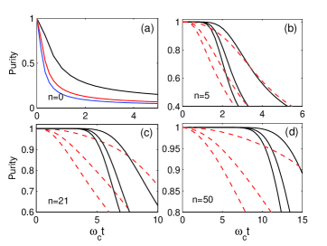
Figure 4: (Color online) Purity defined in Eq. (24) vs time for different number of DD pulse at $T=\omega_{c}$ and $N=200$. Solid lines are for the UDD sequence and dashed lines for the PDD sequence. From the bottom to the top, the curves correspond to $\alpha=0.1,0.05$ and $0.01$.

As discussed in the previous sections, the DD pulses can decouple the state of the system from environment by averaging the decoherence function $R(t)$ to zero. To further check its consequence, here we introduce the purity of a quantum state, which is defined by

$$P(\rho)\equiv\mathrm{Tr}(\rho^{2}).$$ (24)

The quantum state is pure iff its purity takes the maximum value 1, while it is the maximally mixed state $\rho_{m}\equiv\mathbb{I}/D$ iff its purity takes the minimum value $1/D,$ with $D$ the dimensional of quantum system tana .

A comparison of the effects between UDD and PDD sequences for different values of $\alpha$ on protecting the purity of the quantum state is shown in Fig. 4.

Figure 4 indicates the advantage of the UDD sequence in preserving the the purity of quantum state. In contrast to PDD pulses the UDD pulses can preserve the maximum value of purity for a longer time and the behavior for different couplings $\alpha$ do not change as obvious as the case of PDD pulses. This feature of UDD-pulse means it has a long preservation time for maximal purity even with large coupling. Thus, we can obtain a pure state $[P(\rho)=1]$ at certain times if the UDD pulses are applied. It is also indicated that larger number of UDD pulses conduces longer preservation time of pure state.

For a pure state [i.e., $R(t)=0$], based on Eqs. (22) and (23) the maximal QFI can be derived as (see Appendix C)

$$\mathcal{F}_{\max}=N\eta(N,t),$$ (25)

where

$$\eta(N,t) = \max\left\{1+\frac{N-1}{4}\left(A_{+}^{\prime}+\sqrt{A_{+}^{\prime 2}+B^{\prime 2}}\right)\right.,$$ (26)

$$\left.1+\frac{N-1}{2}A_{-}^{\prime}-N\cos^{2N-2}[\Omega(t)]\right\},$$

with

$$A_{\pm}^{\prime} = 1\pm\cos^{N-2}[2\Omega(t)],$$

$$B^{\prime} = -4\sin[\Omega(t)]\cos^{N-2}[\Omega(t)].$$ (27)

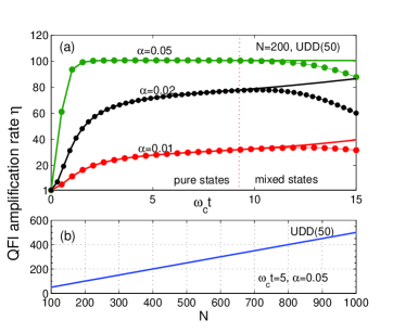
Figure 5: (Color online) (a) QFI amplification rate $\eta$ vs the scaled time $\omega_{c}t$ for different values of coupling strength $\alpha$ with the number of atoms $N=200$. The solid lines are analytical results of pure state, while solid circles line present numerical results of Eq. (20). In the pure states regime they fit well. (b) QFI amplification rate as a function of atom number $N$ at fixed time $\omega_{c}t=5$ with $\alpha=0.05$. The temperature is set as $T=\omega_{c}$ and the number of UDD pulse is $n=50$.

The above equations imply that the maximal QFI can be amplified $\eta$ times compared with CSS in the case of pure states.

In Fig. 5(a), we compare the QFI amplification rate $\eta$ versus scaled time $\omega_{c}t$ between analytical results of pure states and numerical results of actual states with fixed UDD pulse $(n=50)$. It can be seen from Fig. 5(a) that the analytical results are good agreed with the numerical results in the pure states regimes shown in Fig. 4. The amplification is by a factor of 100 for the initial state (CSS) when $\alpha=0.05$ and $N=200$. For $\alpha=0.01$ the amplification is still about a factor of 30. It is indicated that large amplification rate can be easily reached for large $\alpha\$in the presence of UDD pulses. Another interesting behavior is that the large $\alpha$ (such as $\alpha=0.05$) can maintain the QFI unchanged until the quantum state into the mixed states regimes. In the mixed states regimes the amplification rate is reduced, which implies that a larger number of UDD pulses is needed to extend the pure states preservation time, if one wants to maintain the maximal steady amplification rate.

In Fig. 5(b), we plot the QFI amplification rate $\eta$ as a function of atom number $N$ at fixed scaled time $\omega_{c}t=5$. Figure 5(b) shows that the amplification is proportional to the atom number $N$, and the scale factor is $\simeq 1/2$. It indicates that the amplification rate given in Eq. (26) has the maximum value $\eta_{\max}(N)\simeq N/2,$ thus the maximal QFI $\mathcal{F}_{\max}\simeq N^{2}/2$ in this case.

According to the quantum Cramér-Rao theorem, we know that the larger QFI is, the higher precision of estimation is obtained. Thus, the dephasing-induced amplified QFI can greatly improve the the parameter estimation precision; the best result is that it can enhance the phase sensitivity from SQL $\Delta\theta=1/\sqrt{N}$ to $\Delta\theta=\sqrt{2}/N$, which is the same order of magnitude of Heisenberg limit $(1/N)$.

V conclusion

In summary, we have studied the dephasing-assisted PPE enhancement in a two-component BEC system in the presence of DD pulses, through calculating dephasing-induced SS and QFI. It has been found that the dephasing noise can improve PPE by inducing SS. And the DD pulses can maximize the improvement. We have compared the effects between PDD sequence and UDD sequence. Our results showed that the UDD sequence can work more efficiently, which can enhance the decoherence-induced SS to the limit of $\xi^{2}\simeq N^{-2/3}$ more easily and it can amplify the QFI by a factor of $\simeq N/2$ for the initial state of CSS. It implied that the sensitivity $\Delta\theta$ of the estimated parameter $\theta$ can be enhanced from the SQL $1/\sqrt{N}$ to $\sqrt{2}/N$, which achieves nearly Heisenberg-limited precision $(1/N)$.

We would like to mention that, under our consideration, all the $\pi$ control pulses are assumed to execute quickly and perfect, during which the coupling with environment is negligible. Besides, it should be pointed out that, we also have noted that the Heisenberg-limited precision estimation precision have been reached theoretically, via transforming the OAT into “two-axis twisting” YCL ; GJB if some more complex control fields are employed. Finally, we expect that our idea might have promising application in quantum metrology and be realized within current experiments.

Appendix A derivation of the decoherence function $R(t)$

Here, we recap the derivation of the decoherence function $R(t)$ for completeness.

From Eq. (5), the reduced density matrix elements of the system can be read as

$$\rho_{m,n}(t) = \mathrm{Tr}_{B}\left[\left\langle m\right|U(t)\rho(0)U^{-1}(t)\left|n\right\rangle\right]$$

$$= \mathrm{Tr}_{B}\left[\left\langle m\right|e^{-i\phi_{m}}e^{im^{2}\Omega(t)}\exp\left(m\sum_{k}(\alpha_{k}b_{k}^{{\dagger}}-\alpha_{k}^{\ast}b_{k})\right)\right.$$

$$\times \left.\rho(0)e^{i\phi_{n}}e^{-in^{2}\Omega(t)}\exp\left(-n\sum_{k}(\alpha_{k}b_{k}^{{\dagger}}-\alpha_{k}^{\ast}b_{k})\right)\left|n\right\rangle\right]$$

$$= e^{-i(\phi_{m}-\phi_{n})}e^{i(m^{2}-n^{2})\Omega(t)}$$

$$\times \mathrm{Tr}_{B}\left\{\exp\left[(m-n)\sum_{k}(\alpha_{k}b_{k}^{{\dagger}}-\alpha_{k}^{\ast}b_{k})\right]\rho_{B}(0)\right\}\rho_{m,n}(0)$$

with $\alpha_{k}=-ig_{k}\int_{0}^{t}e^{i\omega_{k}s}\epsilon(s)ds.$

To attain the explicit expression of the above equation, the main task becomes to calculate the expectation value of displacement operator

$$\Pi_{k}\mathrm{Tr}_{B}\left[D(z_{k})\rho_{B}\right] = \mathrm{Tr}_{B}\left\{\exp\left[(m-n)\sum_{k}(\alpha_{k}b_{k}^{{\dagger}}-\alpha_{k}^{\ast}b_{k})\right]\rho_{B}\right\}$$

with $z_{k}=(m-n)\alpha_{k}.$

Making use of the following formula hp

$$\mathrm{Tr}_{B}\left[D(z_{k})\rho_{B}\right]=\exp[-(\left\langle n_{k}\right\rangle+1/2)\left|z_{k}\right|^{2}],$$

where $n_{k}=1/(e^{\beta\omega_{k}}-1)$.

Then we arrive at

$$\left\langle D(z_{k})\right\rangle = \mathrm{Tr}_{B}\left[D(z_{k})\rho_{B}\right]$$ (30)

$$= \exp\left[-(m-n)^{2}\left|-ig_{k}\int_{0}^{t}e^{i\omega_{k}s}\epsilon(s)ds\right|^{2}(\left\langle n_{k}\right\rangle+1/2)\right]$$

$$= \exp\left[-(m-n)^{2}\left|g_{k}\right|^{2}\left|\int_{0}^{t}e^{i\omega_{k}s}\epsilon(s)ds\right|^{2}(\left\langle n_{k}\right\rangle+1/2)\right]$$

$$= \exp\left\{-(m-n)^{2}\int_{0}^{\infty}d\omega J(\omega)[2n(\omega)+1]\left|\epsilon(\omega)\right|^{2}/2\right\}$$

$$= \exp\left[-(m-n)^{2}R(t)\right].$$

In the above equation the finite-time Fourier transform $\epsilon(\omega,t)$ of $\epsilon(s)$ can be derived as

$$\epsilon(\omega,t) = \int_{0}^{t}e^{i\omega s}\epsilon(s)ds$$ (31)

$$= \sum_{j=0}^{n}\int_{0}^{t}e^{i\omega s}(-1)^{j}\theta(s-t_{j})\theta(t_{j+1}-s)ds$$

$$= \sum_{j=0}^{n}(-1)^{j}\int_{t_{j}}^{t_{j+1}}e^{i\omega s}ds=\frac{1}{i\omega}\sum_{j=0}^{n}(-1)^{j}[e^{i\omega t_{j+1}}-e^{i\omega t_{j}}]$$

$$= \frac{i}{\omega}\left[1+(-1)^{n+1}e^{i\omega t}+2\sum_{j=1}^{n}(-1)^{j}e^{i\omega t_{j}}\right].$$

Therefore, the decoherence function in Eq. (8) is obtained.

Appendix B derivation of $f(\omega,t)$

In this Appendix, we present details of derivation of Eq. (10). From Eqs. (4) and (10), we have

$$f(\omega,t)=\int_{0}^{t}ds\int_{0}^{s}ds^{\prime}\epsilon(s)\epsilon(s^{\prime})\sin[\omega(s-s^{\prime})]=\frac{1}{2i}[x(\omega,t)-x^{\ast}(\omega,t)]=\mathrm{Im}[x(\omega,t)].$$ (32)

Thus, we obtain

$$x(\omega,t) = \int_{0}^{t}ds\epsilon(s)e^{i\omega s}\int_{0}^{s}ds^{\prime}\epsilon(s^{\prime})e^{-i\omega s^{\prime}}=\sum_{m=0}^{n}\int_{t_{m}}^{t_{m+1}}ds(-1)^{m}e^{i\omega s}\int_{0}^{s}ds^{\prime}\epsilon(s^{\prime})e^{-i\omega s^{\prime}}$$ (33)

$$= \sum_{m=0}^{n}\int_{t_{m}}^{t_{m+1}}ds(-1)^{m}e^{i\omega s}\left[\sum_{j=1}^{m}\int_{t_{j-1}}^{t_{j}}(-1)^{j-1}e^{-i\omega s^{\prime}}ds^{\prime}+(-1)^{m}\int_{t_{m}}^{s}e^{-i\omega s^{\prime}}ds^{\prime}\right]$$

$$= -\frac{i}{\omega}\left\{\sum_{m=0}^{n}\int_{t_{m}}^{t_{m+1}}ds(-1)^{m}e^{i\omega s}\left[1+2\sum_{j=1}^{m}(-1)^{j}e^{-i\omega t_{j}}+(-1)^{m+1}e^{-i\omega s}\right]\right\}$$

$$= -\frac{i}{\omega}\left\{\sum_{m=0}^{n}\int_{t_{m}}^{t_{m+1}}ds(-1)^{m}e^{i\omega s}\left[1+2\sum_{j=1}^{m}(-1)^{j}e^{-i\omega t_{j}}\right]+\sum_{m=0}^{n}\int_{t_{m}}^{t_{m+1}}ds(-1)^{2m+1}\right\}$$

$$= \frac{1}{\omega^{2}}\left[1+(-1)^{n+1}e^{i\omega t}+2\sum_{m=1}^{n}(-1)^{m}e^{-i\omega t_{m}}\right]-\frac{2i}{\omega}\sum_{m=1}^{n}\sum_{j=1}^{m}\int_{t_{m}}^{t_{m+1}}ds(-1)^{m+j}e^{i\omega s}e^{-i\omega t_{j}}+\frac{it}{\omega}$$

$$= \Theta(\omega,t)+\Xi(\omega,t)+\frac{it}{\omega},$$

where

$$\Theta(\omega,t) = \frac{1}{\omega^{2}}\left[1+(-1)^{n+1}e^{i\omega t}+2\sum_{m=1}^{n}(-1)^{m}e^{-i\omega t_{m}}\right],$$

$$\Xi(\omega,t) = -\frac{2}{\omega^{2}}\sum_{m=1}^{n}\sum_{j=1}^{m}(-1)^{m+j}e^{-i\omega t_{j}}(e^{i\omega t_{m+1}}-e^{i\omega t_{m}}).$$ (34)

Then we have

$$f(\omega,t)=\mathrm{Im}[x(\omega,t)]=\mathrm{\vartheta}(\omega,t)+\mathrm{\mu}(\omega,t)+t/\omega,$$ (35)

where

$$\mathrm{\vartheta}(\omega,t)=\mathrm{Im}[\Theta(\omega,t)],\hskip 14.22636pt\mathrm{\mu}(\omega,t)=\mathrm{Im}[\Xi(\omega,t)],$$

which have been given in Eq. (10).

Appendix C QFI of pure states

Based on Eq. (22) of the main text, we have

$$\mathbf{C}=4\left(\begin{array}[]{ccc}(\Delta J_{x})^{2}&\mathrm{Cov}(J_{x},J_{y})&\mathrm{Cov}(J_{x},J_{z})\\ \mathrm{Cov}(J_{x},J_{y})&(\Delta J_{y})^{2}&\mathrm{Cov}(J_{y},J_{z})\\ \mathrm{Cov}(J_{x},J_{z})&\mathrm{Cov}(J_{y},J_{z})&(\Delta J_{z})^{2}\end{array}\right),$$ (36)

with $\mathrm{Cov}(J_{m},J_{n})=\frac{1}{2}\left\langle J_{m}J_{n}+J_{n}J_{m}\right\rangle-\left\langle J_{m}\right\rangle\left\langle J_{n}\right\rangle$.

When the UDD pulses are employed, we have $\phi=J_{z}\int_{0}^{t}\lambda\epsilon(s)ds=0$ in Eq. (7). Following Eq. (7) and Ref. jgr , the expectation values relevant in $\mathrm{Cov}(J_{m},J_{n})$ can be attained as

$$\langle J_{x}J_{y}+J_{y}J_{x}\rangle = \mathrm{Im}\langle J_{+}^{2}\rangle=0,$$

$$\langle J_{x}J_{z}+J_{z}J_{x}\rangle = \mathrm{Re}\langle J_{+}(2J_{z}+1)\rangle=0,$$

$$\langle J_{y}J_{z}+J_{z}J_{y}\rangle = \mathrm{Im}\langle J_{+}(2J_{z}+1)\rangle,$$ (37)

with

$$\langle J_{+}(2J_{z}+1)\rangle=i2j(j-1/2)\cos^{2j-2}(2\Omega)\sin(\Omega),$$

$$\langle J_{+}^{2}\rangle=j(j-1/2)\cos^{2j-2}(2\Omega),\hskip 5.69046pt\langle J_{+}\rangle=j\cos^{2j-1}(\Omega),$$

and

$$\langle J_{x}\rangle = j\cos^{2j-1}(\Omega),\hskip 5.69046pt\langle J_{y}\rangle=\langle J_{z}\rangle=0,\hskip 5.69046pt\langle J_{z}^{2}\rangle=j/2,$$

$$\langle J_{x}^{2}\rangle = \frac{j}{4}(2j+1)+\frac{j}{4}(2j-1)\cos^{2j-2}(2\Omega),$$

$$\langle J_{y}^{2}\rangle = \frac{j}{4}(2j+1)-\frac{j}{4}(2j-1)\cos^{2j-2}(2\Omega).$$ (38)

Hence, the symmetric matrix $\mathbf{C}$ can be rewritten as

$$\mathbf{C}=4\left(\begin{array}[]{ccc}(\Delta J_{x})^{2}&0&0\\ 0&\langle J_{y}^{2}\rangle&\mathrm{Cov}(J_{y},J_{z})\\ 0&\mathrm{Cov}(J_{y},J_{z})&\langle J_{z}^{2}\rangle\end{array}\right)$$ (39)

with the maximal eigenvalue

$$\lambda_{\max}=4\max\{(\Delta J_{x})^{2},\lambda_{\pm}\},$$ (40)

where

$$(\Delta J_{x})^{2} = \frac{N}{4}\left(\frac{N+1}{2}+\frac{N-1}{2}\cos^{2j-2}(2\Omega)-N\cos^{4j-2}(\Omega)\right),$$

$$\lambda_{\pm} = \frac{\left\langle J_{y}^{2}+J_{z}^{2}\right\rangle\pm\sqrt{\left(\left\langle J_{y}^{2}+J_{z}^{2}\right\rangle\right)^{2}+4\mathrm{Cov}(J_{y},J_{z})^{2}}}{2}.$$

References

• (1) T. L. Gustavson, P. Bouyer, and M. A. Kasevich, Phys. Rev. Lett. 78, 2046 (1997).
• (2) J. Fixler, G. Foster, J. McGuirk, and M. Kasevich, Science 315, 74 (2007).
• (3) A. D. Cronin, J. Schmiedmayer, and D. E. Pritchard, Reviews of Modern Physics 81, 1051 (2009).
• (4) C. Gross, T. Zibold, E. Nicklas, J. Estève and M. K. Oberthaler, Nature (London) 464, 1165 (2010).
• (5) M. F. Riedel, P. Böhi, Y. Li, T. W. Hansch, A. Sinatra and P. Treutlein, Nature (London) 464, 1170 (2010).
• (6) N. Bar-Gill, D. D. Bhaktavatsala Rao, and G. Kurizki, Phys. Rev. Lett. 107, 010404 (2011).
• (7) J. Grond, U. Hohenester, I. Mazets, and J. Schmiedmayer, New J. Phys. 12 065036 (2010)
• (8) J. Ma, X. Wang, C. P. Sun, and F. Nori, Phys. Rep. 509, 89 (2011).
• (9) P. Bouyer and M. A. Kasevich, Phys. Rev. A 56, R1083 (1997).
• (10) M. A. Kasevich, Science, 298, 1363 (2002).
• (11) C. Orzel, A. K. Tuchman, M. L. Fenselau, M. Yasuda, M. A. Kasevich, Science 291, 2386 (2001).
• (12) D. J. Wineland, J. J. Bollinger, W. M. Itano, D. J. Heinzen, Phys. Rev. A 50, 67 (1994).
• (13) M. Kitagawa and M. Ueda, Phys. Rev. A 47, 5138 (1993).
• (14) G. R. Jin, Y. C. Liu and W. M. Liu, New J. Phys. 11, 073049 (2009).
• (15) L. Pezze, and A. Smerzi, Phys. Rev. Lett. 102, 100401 (2009).
• (16) Y. C. Liu, Z. F. Xu, G. R. Jin, and L. You, Phys. Rev. Lett. 107, 013601 (2011).
• (17) C. Simon and J. Kempe, Phys. Rev. A 65, 052327 (2002).
• (18) A. Andre and M. D. Lukin, Phys. Rev. A 65, 053819 (2002).
• (19) J. K. Stockton, J. M. Geremia, A. C. Doherty, and H. Mabuchi, Phys. Rev. A 67, 022112 (2003).
• (20) Y. Li, Y. Castin, and A. Sinatra, Phys. Rev. Lett. 100, 210401 (2008).
• (21) A. Sinatra, E.Witkowska, J.-C. Dornstetter, Y. Li, and Y. Castin, Phys. Rev. Lett. 107, 060404 (2011).
• (22) G. Watanabe and H. Makela, Phys. Rev. A 85, 023604 (2012).
• (23) X. Wang, A. Miranowicz, Y. X. Liu, C. P. Sun, F. Nori, Phys. Rev. A 81, 022106 (2010).
• (24) L. Viola and S. Lloyd, Phys. Rev. A 58, 2733 (1998).
• (25) K. Khodjasteh and D. A. Lidar, Phys. Rev. A 75, 062310 (2007).
• (26) G. Gordon and G. Kurizki, Phys. Rev. Lett 97, 110503 (2006); G. Gordon, J. Phys. B: At. Mol. Opt. Phys. 42 223001 (2009).
• (27) G. S. Uhrig, Phys. Rev. Lett. 98, 100504 (2007); New J. Phys. 10, 083024 (2008).
• (28) W. Yang and R. B. Liu, Phys. Rev. Lett. 101, 180403 (2008).
• (29) J. F. Du, X. Rong, N. Zhao, Y. Wang, J. H. Yang, and R. B. Liu, Nature (London) 461, 1265 (2009).
• (30) X. Rong, P. Huang, X. Kong, X. Xu, F. Shi, Y. Wang and J. Du, Europhys. Lett. 95, 60005 (2011).
• (31) A. Z.Chaudhry and J. Gong, Phys. Rev. A 86, 012311 (2012).
• (32) Y. Pan, H. T. Song and Z. R. Xi, J. Phys. B: At. Mol. Opt. Phys. 45 205504 (2012).
• (33) Q. S. Tan, Y. Huang, X. Yin, L. M. Kuang, and X. Wang, Phys. Rev. A 87, 032102 (2013).
• (34) J. M. Taylor, P. Cappellaro, L. Childress, L. Jiang, D. Budker, P. R. Hemmer, A. Yacoby, R.Walsworth and M. D. Lukin, Nature Phys. 4, 810 (2008).
• (35) G. de Lange, D. Ristè, V. V. Dobrovitski, and R. Hanson, Phys. Rev. Lett. 106, 080802 (2011).
• (36) G. Goldstein, P. Cappellaro, J. R. Maze, J. S. Hodges, L. Jiang, A. S. Søensen, and M. D. Lukin, Phys. Rev. Lett. 106, 140502 (2011).
• (37) L. T. Hall, C. D. Hill, J. H. Cole, and L. C. L. Hollenberg, Phys. Rev. B 82, 045208 (2010).
• (38) C. W. Helstrom, Quantum Detection and Estimation Theory (Academic Press, New York, 1976).
• (39) S. L. Braunstein and C. M. Caves, Phys. Rev. Lett. 72, 3439 (1994).
• (40) V. Giovannetti, S. Lloyd, and L.Maccone, Nat. Photonics 5, 222 (2011).
• (41) Z. Sun, J. Ma, X. M. Lu, and X. Wang, Phys. Rev. A 82, 022306 (2010).
• (42) J. Ma, Y. Huang, X. Wang, and C. P. Sun, Phys. Rev. A 84, 022302 (2011).
• (43) G. Ferrini, D. Spehner, A. Minguzzi, and F. W. J. Hekking, Phys. Rev. A 84, 043628 (2011).
• (44) Y. Huang, W. Zhong, Z. Sun, and X. Wang, Rev. A 86, 012320 (2012)
• (45) V. Giovannetti, S. Lloyd, and L. Maccone, Science 306, 1330 (2004); Phys. Rev. Lett 96, 010401 (2006).
• (46) S. F. Huelga, C. Macchiavello, T. Pellizzari, A. K. Ekert, M. B. Plenio, and J. I. Cirac, Phys. Rev. Lett. 79, 3865 (1997). A. W. Chin, S. F. Huelga, and M. B. Plenio, ibid 109, 233601 (2012).
• (47) S.Blanes, F. Casas, J. A. Oteo, and J. Ros, Phys. Rep. 470, 151 (2009).
• (48) L. M. Kuang, Z.Y. Tong, Z. W. Ouyang, and H.S. Zeng, Phys. Rev. A 61, 013608 (1999). J. B. Yuan, L. M. Kuang and J. Q. Liao, J. Phys. B: At. Mol. Opt. Phys. 43 165503 (2010).
• (49) H. P. Breuer and F. Petruccione, The Theory of Open Quantum Systems (Oxford University Press, Oxford, 2002).
• (50) T. Tanaka, G. Kimura, and H. Nakazato, Phys. Rev. A 87, 012303 (2013).