The Geometry of Light Paths
for
Equiangular Spirals

Abstract

First geometric calculus alongside its description of equiangular spirals, reflections and rotations is introduced briefly. Then single and double reflections at such a spiral are investigated. It proves suitable to distinguish incidence from the right and left relative to the radial direction. The properties of geometric light propagation inside the equiangular spiral are discussed, as well as escape conditions and characteristics. Finally the dependence of right and left incidence from the source locations are examined, revealing a well defined inner critical curve, which delimits the area of purely right incident propagation. This critical curve is self similar to the original equiangular spiral.

1 Introduction

Deformations of circular discs lead to new promising laser resonators, dramatically improving output and beam quality [4, 2]. In this paper I want to look at the properties of spiral deformations. In order to do this I will partly apply the very well suited geometric calculus as developed by D. Hestenes and G. Sobczyk [3, 1].

1.1 Prerequisites from Geometric Calculus

Since I am interested in discs, I will only use a real two 2-dimensional Euclidean vector space $\mathcal{E}_{2}$ to represent a plane and its real plane geometric algebra $\mathcal{G}_{2}$. Fundamental for the notion vector in geometric calculus is the associative geometric product of vectors $a$,$b$:

$$\mbox{\boldmath$a$}\mbox{\boldmath$b$}=\mbox{\boldmath$a$}\cdot\mbox{\boldmath$b$}+\mbox{\boldmath$a$}\wedge\mbox{\boldmath$b$}$$ (1)

composed of the conventional scalar inner product $\mbox{\boldmath$a$}\cdot\mbox{\boldmath$b$}$ and the outer product $\mbox{\boldmath$a$}\wedge\mbox{\boldmath$b$}$. $\mbox{\boldmath$a$}\wedge\mbox{\boldmath$b$}$ simply represents the oriented area swept out by $b$, when displaced parallel along $a$ as seen in fig. 1.

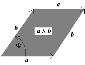
Figure 1: Oriented area $\mbox{\boldmath$a$}\wedge\mbox{\boldmath$b$}$.

There are two orientations in following the outer contours of this area: plus for going first along $a$ and then $b$, etc. and minus for going first along $b$ and then $a$, etc.

Hence, $\mbox{\boldmath$a$}\wedge\mbox{\boldmath$b$}=-\mbox{\boldmath$b$}\wedge\mbox{\boldmath$a$}$. $\mbox{\boldmath$a$}\wedge\mbox{\boldmath$b$}$ is also called a bivector or in this case pseudoscalar, because its rank of 2 is maximal in the plane geometric algebra $\mathcal{G}_{2}$ of scalars(1), vectors(2) and bivectors(1).

The product of two vectors is a spinor. With the help of the oriented unit area element, called ${\mathbf{i}}\in\mathcal{G}_{2}$ it can be written  in exponential form:

$$a b = a\,b\,\,exp({\mathbf{i}}\Phi)$$

$$a = \sqrt{\mbox{\boldmath$a$}\mbox{\boldmath$a$}}=\sqrt{\mbox{\boldmath$a$}^{2}}$$ (2)

$$b = \sqrt{\mbox{\boldmath$b$}^{2}}$$

with ${\mathbf{i}}^{2}=-1$. This property of ${\mathbf{i}}$ can easily be shown by chosing an orthonormal basis in $\mathcal{E}_{2}$: $\{\mbox{\boldmath$\sigma_{1}$},\mbox{\boldmath$\sigma_{2}$}\}$ with $\mbox{\boldmath$\sigma_{1}$}^{2}=\mbox{\boldmath$\sigma_{2}$}^{2}=1;\mbox{\boldmath$\sigma_{1}$}\cdot\mbox{\boldmath$\sigma_{2}$}=0$. ${\mathbf{i}}$ can than be written as ${\mathbf{i}}=\mbox{\boldmath$\sigma_{1}$}\mbox{\boldmath$\sigma_{2}$}=\mbox{\boldmath$\sigma_{1}$}\wedge\mbox{\boldmath$\sigma_{2}$}$. Hence ${\mathbf{i}}^{2}=(\mbox{\boldmath$\sigma_{1}$}\wedge\mbox{\boldmath$\sigma_{2}$})\mbox{\boldmath$\sigma_{1}$}\mbox{\boldmath$\sigma_{2}$}=-(\mbox{\boldmath$\sigma_{2}$}\wedge\mbox{\boldmath$\sigma_{1}$})\mbox{\boldmath$\sigma_{1}$}\mbox{\boldmath$\sigma_{2}$}=-\mbox{\boldmath$\sigma_{2}$}\mbox{\boldmath$\sigma_{1}$}\mbox{\boldmath$\sigma_{1}$}\mbox{\boldmath$\sigma_{2}$}=-\mbox{\boldmath$\sigma_{2}$}\mbox{\boldmath$\sigma_{2}$}=-1$.

Given that both $a$ and $b$ are unit vectors

$$\mbox{\boldmath$a$}\mbox{\boldmath$b$}=exp({\mathbf{i}}\Phi)$$ (3)

can be used to describe the rotation of $a$ into $b$:

$$\mbox{\boldmath$a$}\,\,exp({\mathbf{i}}\Phi)=\mbox{\boldmath$a$}\mbox{\boldmath$a$}\mbox{\boldmath$b$}=\mbox{\boldmath$a$}^{2}\mbox{\boldmath$b$}=\mbox{\boldmath$b$}$$ (4)

Further elements of geometric calculus will be introduced as needed throughout this paper.

1.2 The Equiangular Spiral

A circle of radius $x_{0}$ centered at the origin as shown in fig. 2 may therefore be discribed as

$$\mbox{\boldmath$x$}=\mbox{\boldmath$x_{o}$}exp({\mathbf{i}}\Phi);\Phi\in\mathbf{R}.$$ (5)

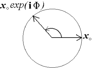
Figure 2: Circle of radius $x_{0}$.

In order to describe an equiangular spiral one needs to add a scalar multiple of $\Phi$ in the exponential:

$$\mbox{\boldmath$x$}=\mbox{\boldmath$x_{o}$}exp({\mathbf{i}}\Phi+t\Phi);\,\,\,\,t=const.\in\mathbf{R}.$$ (6)

The tangent to the curve $\mbox{\boldmath$x$}(\Phi)$ is defined as the first scalar derivative:

$$\partial_{\Phi}\mbox{\boldmath$x$}=\mbox{\boldmath$x_{o}$}exp(({\mathbf{i}}+t)\Phi)({\mathbf{i}}+t)=\mbox{\boldmath$x$}{\mathbf{i}}+\mbox{\boldmath$x$}t$$ (7)

The operation of ${\mathbf{i}}$ on $x$ in (7) is an anticlockwise rotation by a right angle as shown in fig. 3, since

$$exp({\mathbf{i}}\frac{\pi}{2})=cos\frac{\pi}{2}+{\mathbf{i}}sin\frac{\pi}{2}={\mathbf{i}}$$ (8)

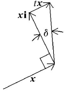
Figure 3: The tangent vector of the equiangular spiral.

It immediately follows that

$$\mid\mbox{\boldmath$x$}{\mathbf{i}}\mid=x\mbox{ and }\mid t\mbox{\boldmath$x$}\mid=tx$$ (9)

and therefore

$$tan\delta=\frac{\mid t\mbox{\boldmath$x$}\mid}{\mid\mbox{\boldmath$x$}{\mathbf{i}}\mid}=t\mbox{ or }\delta=tan^{-1}{}t\,\,(=arctan{}\,\,t)$$ (10)

Hence the tangent $\partial_{\Phi}\mbox{\boldmath$x$}$ has relative to $x$ the angle

$$\frac{\pi}{2}+\delta=\frac{\pi}{2}+tan^{-1}{}t$$ (11)

The deviation of this angle from the case of a pure circle is $\delta=tan^{-1}{}t$ independent of $\Phi$. That is the reason, why the spiral (6) is called equiangular .

Let me assume for the rest of this paper, without loss of generality, that $t>0.$  Such an equiangular spiral with $\delta=0.1(\approx t)$ is shown in fig. 4.

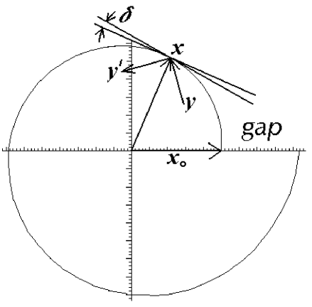
Figure 4: The equiangular spiral for $\delta=0.1$.

2 Reflections at an Equiangular Spiral

2.1 Single Reflections

In order to describe a reflection at the equiangular spiral we need to know the unit normal $n$ at any point $\mbox{\boldmath$x$}(\Phi)$. For a circle the unit normal points in the same direction as the radius vector: $\mbox{\boldmath$n$}=\mbox{{{{\^{x}}}}}$. For an equiangular spiral the tangent vector has the angle $\frac{\pi}{2}+\delta$ relative to x̂. $n$ will hence be equal to x̂ rotated clockwise by $\delta$:

$$\mbox{\boldmath$n$}=\mbox{{{\^{x}}}}exp(-\mathbf{i}\delta)$$ (12)

Every vector $y$ incident at a point $x$ of the equiangular spiral (e.g. representing a light ray to be reflected at $x$) can be uniquely decomposed into components parallel and perpendicular relative to $n$:

$$y = \mbox{\boldmath$y$}_{\|}+\mbox{\boldmath$y$}_{\perp}\mbox{ with }$$

$$\mbox{\boldmath$y$}_{\|} = \mbox{\boldmath$y$}\cdot\mbox{\boldmath$n$}\mbox{\boldmath$n$}$$ (13)

$$\mbox{\boldmath$y$}_{\perp} = \mbox{\boldmath$y$}-\mbox{\boldmath$y$}_{\|}=\mbox{\boldmath$y$}\mbox{\boldmath$n$}\mbox{\boldmath$n$}-\mbox{\boldmath$y$}\cdot\mbox{\boldmath$n$}\mbox{\boldmath$n$}=(\mbox{\boldmath$y$}\mbox{\boldmath$n$}-\mbox{\boldmath$y$}\cdot\mbox{\boldmath$n$})\mbox{\boldmath$n$}=\mbox{\boldmath$y$}\wedge\mbox{\boldmath$n$}\mbox{\boldmath$n$}$$

Here I used the convention that indicated inner and outer products should be performed before an adjacent geometric product (comp. [1], p. 7).

The reflection will then be described by

$$\mbox{\boldmath$y$}^{\prime} = -\mbox{\boldmath$n$}\mbox{\boldmath$y$}\mbox{\boldmath$n$}\stackrel{{\scriptstyle(\ref{eq:vdec})}}{{=}}-\mbox{\boldmath$n$}(\mbox{\boldmath$y$}\cdot\mbox{\boldmath$n$}\mbox{\boldmath$n$}+\mbox{\boldmath$y$}\wedge\mbox{\boldmath$n$}\mbox{\boldmath$n$})\mbox{\boldmath$n$}$$ (14)

$$= (-\mbox{\boldmath$y$}\cdot\mbox{\boldmath$n$}\mbox{\boldmath$n$}-\mbox{\boldmath$n$}\mbox{\boldmath$y$}\wedge\mbox{\boldmath$n$})\mbox{\boldmath$n$}^{2}\stackrel{{\scriptstyle\mbox{\boldmath$n$}^{2}=1}}{{=}}-\mbox{\boldmath$y$}_{\|}+\mbox{\boldmath$y$}_{\perp}$$

In the last step one uses equ. (13) again and the fact that $-\mbox{\boldmath$n$}\mbox{\boldmath$y$}\wedge\mbox{\boldmath$n$}=-\mbox{\boldmath$n$}\wedge(\mbox{\boldmath$y$}\wedge\mbox{\boldmath$n$})-\mbox{\boldmath$n$}\cdot(\mbox{\boldmath$y$}\wedge\mbox{\boldmath$n$})=(\mbox{\boldmath$y$}\wedge\mbox{\boldmath$n$})\cdot\mbox{\boldmath$n$}=(\mbox{\boldmath$y$}\wedge\mbox{\boldmath$n$})\mbox{\boldmath$n$}$. This holds true, because in the geometric algebra $\mathcal{G}_{2}$ the outer product is associative as well and the outer product of two equal vectors is always zero: $-\mbox{\boldmath$n$}\wedge(\mbox{\boldmath$y$}\wedge\mbox{\boldmath$n$})=-\mbox{\boldmath$n$}\wedge\mbox{\boldmath$y$}\wedge\mbox{\boldmath$n$}=\mbox{\boldmath$n$}\wedge\mbox{\boldmath$n$}\wedge\mbox{\boldmath$y$}=0$ . The anticommutativity of the vector $n$ and the bivector $\mbox{\boldmath$y$}\wedge\mbox{\boldmath$n$}$ follows from the general definition of the inner product between vectors $v$ and bivectors $B$ (comp. [1], p. 7):

$$\mbox{\boldmath$v$}\cdot B=\frac{1}{2}(\mbox{\boldmath$v$}B-B\mbox{\boldmath$v$})$$ (15)

With the help of (12) equation (14) can be rewritten as

$$\mbox{\boldmath$y$}^{\prime}=-\mbox{{{\^{x}}}}exp(-\mathbf{i}\delta)\mbox{\boldmath$y$}\mbox{{{\^{x}}}}exp(-\mathbf{i}\delta)=exp(\mathbf{i}\delta)(-\mbox{{{\^{x}}}}\mbox{\boldmath$y$}\mbox{{{\^{x}}}})exp(-\mathbf{i}\delta)$$ (16)

The last equality follows from the fact that in $\mathcal{G}_{2}$ as we just saw, vectors and bivectors anticommute, i.e.

$$\mbox{{{\^{x}}}}\mathbf{i}=-\mathbf{i}\mbox{{{\^{x}}}}$$ (17)

and from expanding $exp(-\mathbf{i}\delta)$ in powers of $-\mathbf{i}\delta$. The inner bracket $(-\mbox{{{\^{x}}}}\mbox{\boldmath$y$}\mbox{{{\^{x}}}})=\mbox{\boldmath$y$}^{\prime}_{c}$ represents according to eq. (14) a reflection at a circle with radius vector x. The two spinors attached to the left and to the right can now both be moved to one side, e.g. as

$$\mbox{\boldmath$y$}^{\prime}=\mbox{\boldmath$y$}^{\prime}_{c}exp(-2\mathbf{i}\delta)$$ (18)

$\mbox{\boldmath$y$}^{\prime}$ is now understood as the composition of the reflection at the circle with radius vector x and a clockwise rotation by the angle of $2\delta$. According to (16) $\mbox{\boldmath$y$}^{\prime}$ may also be written as

$$\mbox{\boldmath$y$}^{\prime}=R^{{\dagger}}{}(-\delta)\mbox{\boldmath$y$}^{\prime}_{c}R(-\delta)\mbox{ with }R(-\delta)=exp(-\mathbf{i}\delta)$$ (19)

Here the ^† operator is the reversion operator, i.e. reversing every geometric product in $R(-\delta)$. That $R^{{\dagger}}{}(-\delta)=R(\delta)$ can easily be seen from the fact that $\mathbf{i}^{{\dagger}}=(\mbox{\boldmath$\sigma_{1}$}\mbox{\boldmath$\sigma_{2}$})^{{\dagger}}=\mbox{\boldmath$\sigma_{2}$}\mbox{\boldmath$\sigma_{1}$}=-\mbox{\boldmath$\sigma_{1}$}\mbox{\boldmath$\sigma_{2}$}=-\mathbf{i}$. Spinors like $R(-\delta)$ are also called rotors, because they elegantly describe rotations. (19) is the double sided spinorial description of rotations (comp. [3], p. 277 ff.).

The increase in angle by $2\delta$ is a clear consequence of the fact, that the tangent of the equiangular spiral is tilted by the constant angle $\delta$ relative to the tangent of a circle with radius vector x.

2.2 Two Successive Reflections

The interesting question to ask is what is the angular difference $\Delta\Phi=\Phi^{\prime}-\Phi$ between two successive reflections. This will also result in an answer to the nontrivial question of how the incident angle for a second successive reflection $\Theta^{\prime\prime}$ depends on the incident angle of the first $\Theta$ as shown in fig. 5. (For a circle we would just have $\Theta=\Theta^{\prime}=\Theta^{\prime\prime}=\Theta^{\prime\prime\prime}$ and $\Delta\Phi=\pi-2\Theta$.) The treatment of this problem naturally splits in the two cases of the second reflection occuring before $(\Phi^{\prime}>\Phi)$ or after $(\Phi^{\prime}<\Phi)$ crossing the gap at $\Phi=2\pi$, i.e. the line segment between $\mbox{\boldmath$x$}_{0}$ and $\mbox{\boldmath$x$}_{2\pi}$. In the following I will distinguish incidence from the right for which the reflected ray leaves the reflecting boundary of the equiangular spiral to the left of the radius vector of the point of reflection, i.e. $\Theta^{\prime}=\Theta+2\delta\in[0,\frac{\pi}{2}+\delta]$, and incidence from the left for which the reflected ray leaves to the right of the radius vector, i.e. $\Theta^{\prime}\in[-\frac{\pi}{2}+\delta,0[$. First, incidence from the right will be treated in detail. It entails the possibility of rays escaping through the gap as will soon be shown. Furthermore incidence from the left can be viewed as the reverse situation of incidence from the right, excluding the possibility of escape.

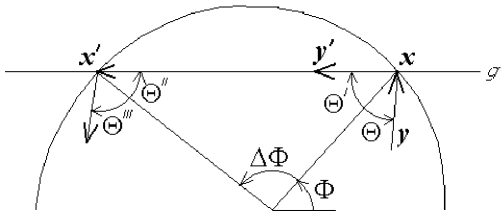
Figure 5: Two successive reflections.

2.2.1 Reflections Without Crossing the Gap

A unit vector of incidence at angle $\Theta$ relative to x̂ is given by

$$\mbox{{{\^{y}}}}=\mbox{{{\^{x}}}}exp(\mathbf{i}\Theta)$$ (20)

The reflected vector is according to (19)

$$\mbox{{{\^{y}}}}^{\prime} = R^{{\dagger}}{}(-\delta)(-\mbox{{{\^{x}}}}\mbox{\boldmath$y$}\mbox{{{\^{x}}}})R(-\delta)=exp(\mathbf{i}\delta)(-\mbox{{{\^{x}}}}\mbox{{{\^{x}}}}exp(\mathbf{i}\Theta)\mbox{{{\^{x}}}})exp(-\mathbf{i}\delta)$$ (21)

$$= -exp(\mathbf{i}(\delta+\Theta))\mbox{{{\^{x}}}}exp(-\mathbf{i}\delta)=\mbox{{{\^{x}}}}exp(-\mathbf{i}(2\delta+\Theta+\pi))$$

In the last step I used the operator identity  $-1=exp(\pm\mathbf{i}\pi)$, i.e. a rotation by $\pi$.

In order to find the location of the second reflection $\mbox{{{x}}}^{\prime}(\Phi^{\prime})$ I construct a straight line $g$ through $x$ with direction $\mbox{{{\^{y}}}}^{\prime}$. $\mbox{{{x}}}^{\prime}(\Phi^{\prime})$ will be its (i.e. the other) point of intersection with the equiangular spiral.

$$g:\mbox{{{y}}}^{\prime} = \mbox{{{x}}}+\lambda\mbox{{{\^{y}}}}^{\prime}=\mbox{\boldmath$x_{o}$}exp(\mathbf{i}\Phi)exp(t\Phi)+\lambda\mbox{{{\^{x}}}}_{\mathbf{0}}exp(\mathbf{i}(\Phi-\Theta-2\delta-\pi))$$ (22)

$$\stackrel{{\scriptstyle!}}{{=}} \mbox{\boldmath$x_{o}$}exp(\mathbf{i}\Phi^{\prime})exp(t\Phi^{\prime})$$

This may be rewritten as

$$\mbox{\boldmath$x_{o}$}exp(\mathbf{i}(\Theta+2\delta))-\lambda\mbox{{{\^{x}}}}_{\mathbf{0}}=\mbox{\boldmath$x_{o}$}exp(t(\Phi^{\prime}-\Phi)exp(\mathbf{i}(\Phi^{\prime}-\Phi+\Theta+2\delta))$$ (23)

Multiplication with $\mbox{\boldmath$x_{o}$}^{-1}=\frac{\mbox{\boldmath$x_{o}$}}{\textstyle x_{0}^{2}}$ from the left gives:

$$exp(\mathbf{i}\Theta^{\prime})-\frac{\lambda}{x_{0}}=exp(t\Delta\Phi)exp(\mathbf{i}(\Delta\Phi+\Theta^{\prime}))$$ (24)

where $\Theta^{\prime}=\Theta+2\delta$ as we have seen in section 2.1.

Equation (24) has scalar and bivector parts, which must be satisfied separately. The bivector part divided by $\mathbf{i}$ reads

$$sin\Theta^{\prime}=exp(t\Delta\Phi)sin(\Delta\Phi+\Theta^{\prime})$$ (25)

(25) is a transcendental equation for $\Phi^{\prime}=\Delta\Phi+\Phi$ which may either be solved graphically or numerically with Newton iteration. For the graphical solution it is convenient to multiply (25) with $exp(t\Theta^{\prime})$:

$$f(\Delta\Phi+\Theta^{\prime}):=exp(t(\Delta\Phi+\Theta^{\prime}))sin(\Delta\Phi+\Theta^{\prime})=exp(t\Theta^{\prime})sin(\Theta^{\prime})=:f(\Theta^{\prime})$$ (26)

$f$ is a simple sinus function with an exponential envelope $exp(t\Theta^{\prime})$ depending on the parameter $t=tan\delta$. (For the circle t = 0 and therefore $exp(t\Theta^{\prime})\equiv 1$.)

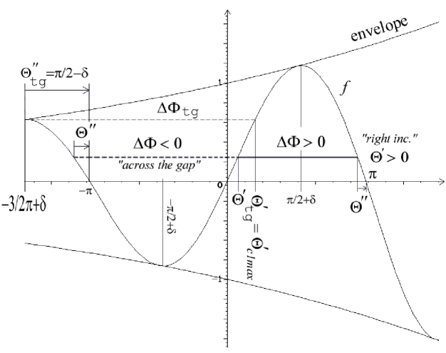
Figure 6: Graphical solution for successive reflections of right incident ray.

For the circle we have $\Theta^{\prime}=\Theta^{\prime\prime}$. Yet for the equiangular spiral the upper right half of fig. 6 clearly shows that $\Theta^{\prime}\geq\Theta^{\prime\prime}$, since the envelope $exp(t\Theta^{\prime})$ is a monotone increasing function of $\Theta^{\prime}$. It is however possible to show, that

$$\Theta<\Theta^{\prime\prime}\mbox{ for }\Theta\in[-2\delta,\frac{\pi}{2}-\delta[.$$ (27)

Before proving this let me first establish another useful property of the $\Theta^{\prime\prime}(\Theta)$ dependence:

$$\frac{\partial\Theta^{\prime\prime}}{\partial\Theta}>0\mbox{ for }\Theta\in[-2\delta,\frac{\pi}{2}-\delta[.$$ (28)

which shows that $\Theta^{\prime\prime}$ is a monotone increasing function of $\Theta$ in $\Theta\in[-2\delta,\frac{\pi}{2}-\delta[$.

Proof of Eq. (28)

Since according to fig. 5 $\Theta^{\prime\prime}=\pi-(\Delta\Phi+\Theta^{\prime})$ we may write eq. (26) as

$$\mbox{{\~{h}}}(\Theta^{\prime\prime}):=exp(t(\pi-\Theta^{\prime\prime}))sin\Theta^{\prime\prime}=exp(t(\Theta+2\delta))sin(\Theta+2\delta)=:\mbox{{\~{f}}}(\Theta)$$ (29)

Therefore

$$\frac{\partial\Theta^{\prime\prime}}{\partial\Theta}=\frac{\partial\mbox{{\~{f}}}}{\partial\Theta}\left(\frac{\partial\mbox{{\~{h}}}}{\partial\Theta^{\prime\prime}}\right)^{-1}$$ (30)

Differentiation of f̃ and h̃ respecively gives

$$\frac{\partial\mbox{{\~{f}}}}{\partial\Theta} = \mbox{{\~{f}}}(\Theta)(tan\delta+\frac{1}{tan(\Theta+2\delta)})$$

$$\frac{\partial\mbox{{\~{h}}}}{\partial\Theta^{\prime\prime}} = \mbox{{\~{h}}}(\Theta^{\prime\prime})(-tan\delta+\frac{1}{tan\Theta^{\prime\prime}})$$ (31)

According to (30) and (29) this results in

$$\frac{\partial\Theta^{\prime\prime}}{\partial\Theta}=\frac{1+\frac{1}{tan(\Theta+2\delta)tan\delta}}{-1+\frac{1}{tan\Theta^{\prime\prime}{}tan\delta}}$$ (32)

The numerator of the rhs. of eq. (32) equals

$$\frac{1+tan^{2}{}\delta}{tan(\Theta+\delta)+tan^{2}{}\delta}>0\mbox{ for }\Theta\in[-2\delta,\frac{\pi}{2}-\delta[,$$ (33)

whilst the supremum value  of $tan\Theta^{\prime\prime}$ in the nominator of the same equation can be written as

$$tan\Theta^{\prime\prime}_{\mathit{sup}}=tan(\frac{\pi}{2}-\delta)=\frac{1}{tan\delta}.$$ (34)

Hence $tan\Theta^{\prime\prime}tan\delta<1$ and $-1+\frac{1}{tan\Theta^{\prime\prime}{}tan\delta}>0$ for $\Theta\in[-2\delta,\frac{\pi}{2}-\delta[$ and $\Theta^{\prime\prime}\in[0,\frac{\pi}{2}-\delta[$ respectively. This conludes the proof of eq. (28) since now both the numerator and the nominator of eq. (32) are proven to be positive for $\Theta\in[-2\delta,\frac{\pi}{2}-\delta[$ and $\Theta^{\prime\prime}\in[0,\frac{\pi}{2}-\delta[$ respectively.

Let me finally remark that for the case of tangential incidence (at the inside of the equiangular spiral) with $\Theta=\Theta^{\prime\prime}=\frac{\pi}{2}-\delta$ we obviously have $\Delta\Phi=0$.

Proof of Eq. (27): $\Theta<\Theta^{\prime\prime}$

For the other extreme of $\Theta=-2\delta$ and $\Theta^{\prime}=\Theta+2\delta=0$ we have according to eq. (29) and figs. 5 and 6 respectively, $\Theta^{\prime\prime}=0$, i.e.

$$\Theta<\Theta^{\prime\prime}\mbox{ for }\Theta=-2\delta$$ (35)

Based on this, the most important step of the proof will be to first show that $\Theta\neq\Theta^{\prime\prime}$ for $\Theta\in[-2\delta,\frac{\pi}{2}-\delta[$. Because $\Theta^{\prime\prime}$ is a continuous differentiable function of $\Theta$ in this interval, it will then immediately follow from eq. (35) that $\Theta<\Theta^{\prime\prime}$ for all $\Theta\in[-2\delta,\frac{\pi}{2}-\delta[$. That $\Theta^{\prime\prime}(\Theta)$ is continuous and differentiable is evident from the analytic expression for $\frac{\partial\Theta^{\prime\prime}}{\partial\Theta}$ given in eq. (32), which is well defined for $\Theta\in[-2\delta,\frac{\pi}{2}-\delta[$.

It now remains to show, that $\Theta\neq\Theta^{\prime\prime}$ for $\Theta\in[-2\delta,\frac{\pi}{2}-\delta[$. I will start out supposing the opposite, i.e. $\Theta=\Theta^{\prime\prime}$ for some $\Theta\in[-2\delta,\frac{\pi}{2}-\delta[$ and show that this leads to contradictions. Supposing that for some $\Theta\in[-2\delta,\frac{\pi}{2}-\delta[$ I would have $\Theta=\Theta^{\prime\prime}$, I can rewrite eq. (25) as

$$exp(t(\pi-\Theta))sin\Theta-exp(t(\Theta+2\delta))sin(\Theta+2\delta)=0$$ (36)

I will examine the validity of (36) first in the intervall $\Theta\in[-2\delta,0[$, then at the point $\Theta=0$ and finally for $\Theta\in]0,\frac{\pi}{2}-\delta[$.

First for $\Theta\in[-2\delta,0[$ we have $exp(t(\pi-\Theta))sin\Theta<0$ and $exp(t(\Theta+2\delta))sin(\Theta+2\delta)\geq 0$. Therefore the expression on the lhs. of eq. (36) will be

$$exp(t(\pi-\Theta))sin\Theta-exp(t(\Theta+2\delta))sin(\Theta+2\delta)<0\mbox{ for }\Theta\in[-2\delta,0[$$ (37)

which is in contradiction to eq. (36). Hence we have

$$\Theta\neq\Theta^{\prime\prime}\mbox{ for }\Theta\in[-2\delta,0[$$ (38)

Second for $\Theta=0$ the lhs. of eq. (36) becomes

$$-exp(t2\delta)sin2\delta\neq 0\mbox{ for }0<\delta<\frac{\pi}{2}$$ (39)

in contradiction to eq. (36). Hence I conlude again, that

$$\Theta\neq\Theta^{\prime\prime}\mbox{ for }\Theta=0$$ (40)

(I am not concerned  with $\delta=0$, i.e. the circle or $\delta=\frac{\pi}{2}$, i.e. a straight half line in the direction of $\mbox{{{\^{x}}}}_{\mathbf{0}}$ beginning at $x_{o}$, nor with $\delta>\frac{\pi}{2}$, which is equivalent to an equiangular spiral winding clockwise with $\delta^{\prime}=\pi-\delta$.)

Finally for $\Theta\in]0,\frac{\pi}{2}-\delta[$ I will calculate the first derivative of the lhs. of eq. (36) with respect to $\Theta$:

$$\frac{\partial}{\partial\Theta}\left(exp(t(\pi-\Theta))sin\Theta-exp(t(\Theta+2\delta))sin(\Theta+2\delta)\right)$$ (41)

$$= -exp(t(\pi-\Theta))(t\,sin\Theta-cos\Theta)$$

$$-exp(t(\Theta+2\delta))(t\,sin(\Theta+2\delta)+cos(\Theta+2\delta))$$

$$\stackrel{{\scriptstyle t=\frac{sin\delta}{cos\delta}}}{{=}} -\frac{exp(t(\pi-\Theta))}{cos\delta}(sin\delta\,\,sin\Theta-cos\delta\,\,cos\Theta)$$

$$-\frac{exp(t(\Theta+2\delta))}{cos\delta}(sin\delta\,\,sin(\Theta+2\delta)+cos\delta\,\,cos(\Theta+2\delta))$$

$$= \frac{1}{cos\delta}(exp(t(\pi-\Theta))cos(\Theta+\delta)-exp(t(\Theta+2\delta))cos(\Theta+\delta))$$

$$= \frac{cos(\Theta+\delta)}{cos\delta}exp(t(\Theta+2\delta))(exp(t(\pi-2(\Theta+\delta)))-1)$$

$$> 0\,\,\,\,\mbox{ for }\Theta\in]0,\frac{\pi}{2}-\delta[$$

The last inequality holds, because both $\frac{cos(\Theta+\delta)}{cos\delta}exp(t(\Theta+2\delta))>0$ and $(\pi-2(\Theta+\delta))>0$ hold for $\Theta\in]0,\frac{\pi}{2}-\delta[$. I therefore conlude, that the lhs. of eq. (36) is a stricly monotone increasing function of $\Theta$. This means that it will not vanish for any $\Theta\in]0,\frac{\pi}{2}-\delta[$ because at the supremum of $\Theta_{\mathit{sup}}=\frac{\pi}{2}-\delta$ of the intervall $]0,\frac{\pi}{2}-\delta[$ the lhs. of eq. (36) (and its first derivative with respect to $\Theta$) is actually zero. The nonvanishing of the lhs. of eq. (36) for $\Theta\in]0,\frac{\pi}{2}-\delta[$ contradicts eq. (36) and hence the supposition $\Theta=\Theta^{\prime\prime}$ for any $\Theta\in]0,\frac{\pi}{2}-\delta[$. I conlude that

$$\Theta\neq\Theta^{\prime\prime}\mbox{ for }\Theta\in]0,\frac{\pi}{2}-\delta[$$ (42)

Taking eqs. (38), (40) and (42) together it is shown that $\Theta\neq\Theta^{\prime\prime}$ for $\Theta\in[-2\delta,\frac{\pi}{2}-\delta[$. This conludes the prove for eq. (27) as argued above.

Indeed, eq. (27) holds not only for $\Theta^{\prime}\in[0,\frac{\pi}{2}+\delta[$ and reflections which don‘t cross the gap radius between the origin and $\mbox{\boldmath$x$}_{2\pi}$, but also if the gap radius is crossed by a ray. The left side of fig. 6 will be explained in section 2.2.2. Anticipating this and refering in addition to fig. 7, fig. 6 shows that because of the strictly monotone character of the exponential envelope $\Theta^{\prime\prime}>\Theta^{\prime}(=\Theta+2\delta)$ holds. Hence we immediately end up with

$$\Theta^{\prime\prime}>\Theta$$

for right incident rays travelling across the gap as well. Therefore eq. (27) holds in full generality for any right incident ray.

The property $\Theta<\Theta^{\prime\prime}$ physically means that successive reflections of light rays incident from the right bend the paths of these rays closer and closer to the tangential direction of $\partial_{\Phi}\mbox{\boldmath$x$}$, i.e. to the equiangular spiral disc boundary.

After infering all these properties from eq. (25) a comment on its familiar geometric meaning is in place. Because

$$sin(\Delta\Phi+\Theta^{\prime}) = sin(\pi-(\Delta\Phi+\Theta^{\prime}))=sin\Theta^{\prime\prime}\mbox{ and }$$

$$exp(t\Delta\Phi) = \frac{exp(t\Phi^{\prime})}{exp(t\Phi)}=\frac{x^{\prime}}{x}$$

we can rewrite eq. (25) as

$$x^{\prime}sin\Theta^{\prime\prime}=xsin\Theta^{\prime}$$ (43)

Looking at the angles in fig. 5 we see that eq. (25) in the form of eq. (43) embodies nothing else but the familiar law of sinuses of the triangle formed by the side vectors $x$ and $\mbox{\boldmath$x$}^{\prime}$.

2.2.2 Reflecting Across the Gap

What happens now, if a refelcted ray actually crosses the $\Phi=2\pi$ radius, i.e. the line segment between the origin and $\mbox{\boldmath$x$}_{2\pi}$ part of which forms the gap?

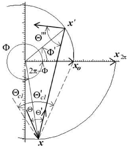
Figure 7: Successive reflections across the gap.

As may readily be seen from fig. 7, a ray passing the angle $\Phi=2\pi$ may continue to be reflected inside the equiangular spiral, for angles of incidence from the right of less than a critical angle $\Theta_{c1}$, which remains to be determined. Or it may eventually emanate from the spiral for $\Theta>\Theta_{c1}$.

Eq. (25) holds for this case equally. The only difference is that we now have to deal with a negative $\Delta\Phi=\Phi^{\prime}-\Phi$, since $\Phi^{\prime}<\Phi$. In fig. 6 this case is represented by the dashed line extending from $f(\Theta^{\prime})$ to the left. Where this line intersects $f$ again, somewhere in the intervall $\Delta\Phi+\Theta^{\prime}\in[-\pi,-\frac{3}{2}\pi+\delta[$ we have $f(\Delta\Phi+\Theta^{\prime})$. The negative length of this horizontal line segment is precisely $\Delta\Phi$. The sum of angles in the triangle formed by the origin, $\mbox{\boldmath$x$}(\Phi)$ and $\mbox{\boldmath$x$}(\Phi^{\prime})$ gives

$$\Theta^{\prime\prime}+\Theta^{\prime}+\Delta\Phi=-\pi.$$ (44)

Hence the representation of $\Theta^{\prime\prime}$, the angle of incidence at $\Phi^{\prime}$, as drawn in fig. 6.

2.2.3 The Condition of Escape

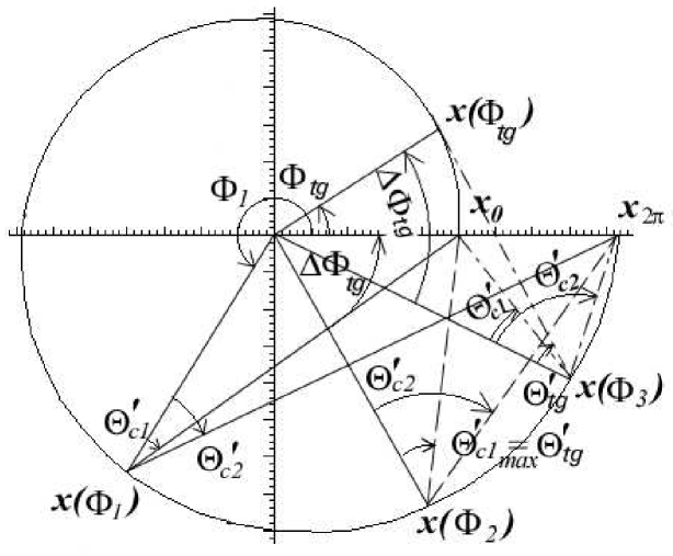
Figure 8: Angular conditions of escape.

First for $0<\Theta^{\prime}<\Theta^{\prime}_{c1}(\Phi)$ a light ray will continue to go round anticlockwise inside the spiral.

Second for

$$\Theta^{\prime}_{c1}(\Phi)<\Theta^{\prime}<\Theta^{\prime}_{c2}(\Phi)$$ (45)

a light ray will leave the spiral straight away (comp. Fig. 12).

And third for $\Theta^{\prime}>\Theta^{\prime}_{c2}(\Phi)$ a ray will experience further reflections between $\mbox{\boldmath$x$}(\Phi)$ and $\mbox{\boldmath$x$}(2\pi)$ along the equiangular spiral boundary until it finally leaves the equiangular spiral without reentering the anticlockwise polygonal motion of the rays of the first case.

$\Theta^{\prime}_{c1}(\Phi)$ (second incidence at $x_{0}$) can be determined from eq. (25) by inserting $\Phi^{\prime}=0$:

$$exp(t(-\Phi+\Theta^{\prime}_{c1}))sin(-\Phi+\Theta^{\prime}_{c1})=exp(t\Theta^{\prime}_{c1})sin\Theta^{\prime}_{c1}.$$ (46)

Likewise $\Theta^{\prime}_{c2}(\Phi)$ (second incidence at $\mbox{\boldmath$x$}(2\pi)$) can be determined from eq. (25) by inserting $\Phi^{\prime}=2\pi$:

$$exp(t(2\pi-\Phi+\Theta^{\prime}_{c2}))sin(2\pi-\Phi+\Theta^{\prime}_{c2})=exp(t\Theta^{\prime}_{c2})sin\Theta^{\prime}_{c2}.$$ (47)

Eq. (46) can be used to graphically determine $\Theta^{\prime}_{c1}$ with the help  of fig. 6: Set $\Delta\Phi=-\Phi$ for a given $\Phi$. For $\Delta\Phi<-\pi$ we fit a (dashed) horizontal line segment of length $\Delta\Phi$ between $f(\Theta^{\prime})$ to the right and $f(\Delta\Phi+\Theta^{\prime})$ to the left. The $\Theta^{\prime}$, where the segment touches the curve $f(\Theta^{\prime})$ is $\Theta^{\prime}_{c1}$. (The corresponding cricital angle of incidence at $\mbox{\boldmath$x$}(\Phi)$ is $\Theta_{c1}=\Theta^{\prime}_{c1}-2\delta$.)

By similarly fitting an (unbroken) horizontal line segment of length $\Delta\Phi=2\pi-\Phi>0$ between $f(\Theta^{\prime})$ to the left and $f(\Delta\Phi+\Theta^{\prime})$ to the right in fig. 6 we can determine $\Theta^{\prime}_{c2}$ (and $\Theta_{c2}$ respectively).

For rays which fulfil the condition of straight escape (45), one can further distinguish, whether they reflect a last time at the outer side of the equiangular spiral or not. This is essential for deciding the asymptotic directions of light rays leaving the gap of the equiangular spiral.

The criterion for this may also be derived from eq. (25). Tangential incidence at the outer side of the equiangular spiral occurs for $\Theta^{\prime}_{c1}<\Theta^{\prime}_{tg}$ with $\Theta^{\prime\prime}_{tg}=\frac{\pi}{2}-\delta$. The point of tangential incidence on the outer side at $\Phi_{tg}$ can be determind graphically from fig. 6. $\Delta\Phi_{tg}=\Phi_{tg}-\Phi<0$ is given by the horizontal distance between the maximum of $f$ to the left (at $\Theta^{\prime\prime}_{tg}=\frac{\pi}{2}-\delta$) and $f(\Theta^{\prime})$ to the right. The point on $f(\Theta^{\prime})$, where this (dashed) horizontal line ends is $\Theta^{\prime}_{tg}$. In case that $\Theta^{\prime}_{c1}<\Theta^{\prime}_{tg}$ the intervall $\Theta^{\prime}_{c1}<\Theta^{\prime}<\Theta^{\prime}_{c2}$ can be subdivided into $\Theta^{\prime}_{c1}<\Theta^{\prime}<\Theta^{\prime}_{tg}$, for which rays leaving straight will reflect a last time at the outer side of the spiral and $\Theta^{\prime}_{tg}<\Theta^{\prime}<\Theta^{\prime}_{c2}$, for which rays leave straight without further incidence at the outside.

The latter kind of rays will actually leave the gap under an angle $\Phi_{e}$ relative to the direction of $\mbox{{{\^{x}}}}_{\mathbf{0}}$ given by

$$\Phi_{e}=\Phi-\pi-\Theta^{\prime}$$ (48)

and an abscissa of escape $x_{e}$ given by

$$x_{e}=x\frac{sin\Theta^{\prime}}{sin\Phi_{e}}$$ (49)

as can be seen from fig. 9.

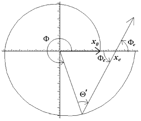
Figure 9: Angle and abscissa of escape.

This actually characterizes the asymptotic radiation completely in case that one ignores the reflection of rays at the outside, e.g. because of absorption.

2.3 Incidence from the Left

As for incidence from the left, i.e. $0>\Theta^{\prime}\geq-\frac{\pi}{2}+\delta$, eq. (25) now describes the graph of $f$ in the lower part of fig. 6 with negative values of the ordinate. This is redrawn in fig. 11.

The angular position of $\mbox{{{x}}}_{0}$ relative to x as illustrated in fig. 10 tells whether a ray will cross the radial position $\Phi=2\pi$ of the gap or not. For $\Theta^{\prime}<\Theta^{\prime}_{cl}$ the ray reflected at $\mbox{{{x}}}(\Phi)$ will not cross the gap and the unbroken horizontal line segment extending between $f(\Theta^{\prime})$ to the right and $f(\Theta^{\prime}+\Delta\Phi)$ to the left applies. For $\Theta^{\prime}>\Theta^{\prime}_{cl}$ the reflected ray will cross the gap and the dashed horizontal line segment extending between $f(\Theta^{\prime})$ to the left and $f(\Theta^{\prime}+\Delta\Phi)$ to the right applies.

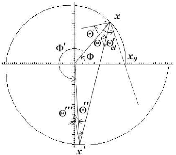
Figure 10: Incidence from the left.

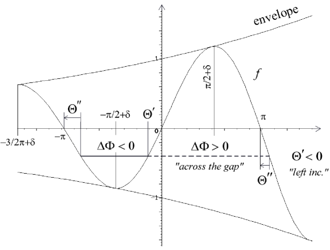
Figure 11: Graphical solution for successive reflections of left incident ray.

Another way to view rays which are incident from the left is as the reverse of corresponding rays incident from the right. According to fig. 5 this would mean to mutually exchange $\Phi$ and $\Phi^{\prime}$, $\Theta$ and $\Theta^{\prime\prime\prime}$, and $\Theta^{\prime}$ and $\Theta^{\prime\prime}$:

$$\Phi\leftrightarrow\Phi^{\prime};\Theta\leftrightarrow\Theta^{\prime\prime\prime};\Theta^{\prime}\leftrightarrow\Theta^{\prime\prime}.$$ (50)

Applying this to the inequality (27) as well we get

$$\Theta^{\prime\prime}-2\delta=\Theta^{\prime\prime\prime}<\Theta^{\prime}=\Theta-2\delta\mbox{ for }\Theta^{\prime}\in[0,\frac{\pi}{2}-\delta[$$

or adding $2\delta$

$$\Theta^{\prime\prime}<\Theta\mbox{ for }\Theta\in[2\delta,\frac{\pi}{2}+\delta[$$ (51)

This means that light rays with incidence from the left will be bent closer and closer to the radial direction x̂ as they perform a clockwise polygonal motion through the equiangular sprial. Once $\Theta^{\prime\prime}$ has become smaller than $2\delta$ they can be treated as rays with incidence from the right with $\Theta\in[-2\delta,\frac{\pi}{2}-\delta[$ as described earlier in section  2.2. In particular, as long as a ray remains in the ‘incidence from the left’ state, it will not leave through the gap at $\Phi=2\pi$. Only after it evolves into an ‘incidence from the right’ state, it will eventually escape.

3 Dependence on the Source Location Inside the Equiangular Spiral

Depending on where the source $x_{s}$ of a light ray is situated and in which direction it is emitted, it will at its first point of reflection $x$ either be incident from the right or possibly from the left relative to $\mbox{{{\^{x}}}}(\Phi)$. An illustration of this is given in fig. 12.

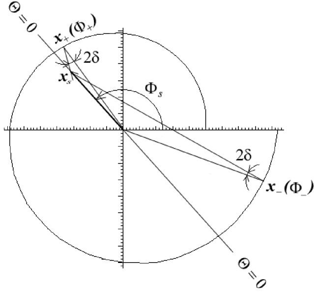
Figure 12: Sectors of incidence from the right (and left).

Fig. 12 shows, that depending on the source location $x_{s}$ there are in principle two sectors: for all $\mbox{{{{x}}}}(\Phi)$ on the equiangular spiral in the region $\Phi\in[\Phi_{+},\Phi_{-}[$ rays emitted from $x_{s}$ will appear to be incident from the right relative to $\mbox{{{\^{x}}}}(\Phi)$, whilst for all $\mbox{{{{x}}}}(\Phi)$ on the equiangular spiral with $\Phi\in[\Phi_{-},2\pi[$ or $\Phi\in[0,\Phi_{+}[$ rays emitted from $x_{s}$ will appear to be incident from the left relative to $\mbox{{{\^{x}}}}(\Phi)$. $\Phi_{+}$ and $\Phi_{-}$ will both be functions of $\Phi_{s}$ and $x_{s}$, determined by the condition $\Theta=-2\delta$.

In the plane geometric algebra $\mathcal{G}_{2}$ this may be expressed by

$$\mbox{{{\^{x}}}}_{\pm}{}\mbox{{{\^{r}}}}_{\pm} = exp(-2\mathbf{i}\delta)$$ (52)

$$\mbox{where \hskip 28.45274pt }\mbox{{{r}}}_{\pm} = \mbox{{{x}}}_{\pm}-\mbox{\boldmath$x_{s}$},$$ (53)

$$\mbox{{{{x}}}}_{\pm} = \mbox{\boldmath$x_{0}$}exp((\mathbf{i}+t)\Phi_{\pm})$$ (54)

$$\mbox{and \hskip 28.45274pt }\mbox{{{{x}}}}_{s} = x_{s}\frac{\mbox{\boldmath$x_{0}$}}{x_{0}}exp(\mathbf{i}\Phi_{s})$$

Inserting $\mbox{{{\^{r}}}}_{\pm}=\mbox{{{r}}}_{\pm}/r_{\pm}$ and $\mbox{{{\^{x}}}}_{\pm}=\mbox{{{x}}}_{\pm}/x_{\pm}$ into eq. (52) we get:

$$x_{\pm}^{2}-\mbox{{{x}}}_{\pm}\mbox{{{x}}}_{s}=x_{\pm}\mid\mbox{{{x}}}_{\pm}-\mbox{{{x}}}_{s}\mid exp(-2\mathbf{i}\delta)$$ (55)

divided by $x_{\pm}$ this gives

$$x_{\pm}-\frac{\mbox{{{x}}}_{\pm}\mbox{{{x}}}_{s}}{x_{\pm}}=\mid\mbox{{{x}}}_{\pm}-\mbox{{{x}}}_{s}\mid exp(-2\mathbf{i}\delta).$$ (56)

Inserting now (54) results in

$$x_{0}exp(t\Phi_{\pm})-\frac{1}{x_{o}exp(t\Phi_{\pm})}\mbox{\boldmath$x_{0}$}exp(\mathbf{i}\Phi_{\pm})exp(t\Phi_{\pm})\frac{x_{s}}{x_{0}}\mbox{\boldmath$x_{0}$}exp(\mathbf{i}\Phi_{s})$$

$$=\mid\mbox{{{x}}}_{\pm}-\mbox{{{x}}}_{s}\mid exp(-2\mathbf{i}\delta).$$ (57)

By interchanging $x_{0}$ and $exp(\mathbf{i}\Phi_{\pm})$ and multiplying both sides with$exp(2\mathbf{i}\delta)/x_{0}$ we get

$$exp(t\Phi_{\pm})exp(2\mathbf{i}\delta)-\frac{x_{s}}{x_{0}}\frac{\mbox{\boldmath$x_{0}$}^{2}}{x_{0}^{2}}exp(\mathbf{i}(\Phi_{s}-\Phi_{\pm}+2\delta))=\frac{\mid\mbox{{{x}}}_{\pm}-\mbox{{{x}}}_{s}\mid}{x_{0}}$$ (58)

The bivector part of this equation divided by i reads

$$exp(t\Phi_{\pm})sin2\delta-\frac{x_{s}}{x_{0}}sin(\Phi_{s}-\Phi_{\pm}+2\delta)=0$$ (59)

which is equivalent to

$$exp(t\Phi_{\pm})=\frac{x_{s}}{x_{0}}\frac{sin(\Phi_{s}-\Phi_{\pm}+2\delta)}{sin2\delta}$$ (60)

Equation (60) is a transcendental equation for $\Phi_{+}$ and $\Phi_{-}$ depending on three parameters: $\delta$ the angle between the radial direction x̂ and the outer normal $n$, $\Phi_{s}$ and $x_{s}$ the polar coordinates of the source $x_{s}$. A close look reveals, that eq. (60) just expresses the law of sinuses in the triangles formed by the side vectors $x_{s}$ and $x_{+}$ or $x_{-}$ respectively, since the lhs. $exp(t\Phi_{\pm})$ is equal to the relative amplitudes $\frac{x_{\pm}}{x_{0}}$.

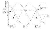
Figure 13: $\Phi_{+}$ and $\Phi_{-}$ as functions of the polar angle of the source $\Phi_{s}$ for constant $\frac{x_{s}}{x_{0}}=0.7$ and $\delta=0.1$.

Fig. 13 shows the rhs. of eq. (60) for constant $x_{s}$ and varying values of $\Phi_{s}$. The points of intersection of the sinusoidal curves with the exponential function $exp(t\Phi)$ gives the desired two pairs of values ($x_{\pm},\Phi_{\pm}$).

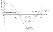
Figure 14: $\Phi_{+}$ and $\Phi_{-}$ as functions of the radial location of the source $x_{s}$ for constant $\Phi_{s}=2\,rad$ and $\delta=0.1$.

Fig. 14 shows the rhs. of eq. (60) as well, but this time for fixed $\Phi_{s}$ and varying $x_{s}$. It can be seen that there will be a certain critical value $x_{s}=x_{cs}$, where the sinussoidal curves representing the rhs. of eq. (60) just touch the lhs. amplitude function $exp(t\Phi)$ only once, hence $x_{+}=x_{-}=x_{c\pm}$ and $\Phi_{+}=\Phi_{-}=\Phi_{c\pm}$ . For $x_{s}<x_{cs}$, all the rays emitted from $x_{s}$ will be incident from the right at points of the equiangular spiral.

I think therefore that the values of $x_{cs}{(\Phi_{s})}$ deserve further attention. As it will turn out, an analytical expression for $x_{cs}{(\Phi_{s})}$ can be derived. I will treat this problem first. In the following I will call the set of points given by $x_{cs}{(\Phi_{s})}$ simply: $x_{cs}$.

3.1 The Critical Curve of Source Locations $x_{s}$

The condition for $x_{cs}$ expressed in the above can be mathematically formulated as equation (60) and

$$\frac{\partial}{\partial\Phi}exp(t\Phi)\mid_{\Phi=\Phi_{c\pm}}=\frac{x_{s}}{x_{0}}\frac{1}{sin2\delta}\frac{\partial}{\partial\Phi}sin(\Phi_{s}-\Phi+2\delta)\mid_{\Phi=\Phi_{c\pm}}$$ (61)

i.e. the lhs. and the rhs. of eq. (60) must be equal as well as their first derivatives with respect to $\Phi$. $\Phi_{s}$ in eq. (61) is the independent variable upon which $x_{s}$ depends. The value of $x_{s}$ fulfilling eqs. (60) and (61) will be the desired $x_{cs}{(\Phi_{s})}$.

Performing the differentiation in eq. (61) and dividing the resulting lhs. by $exp(t\Phi)$ and the resulting rhs. by the rhs. of (60) we obtain

$$t=-\frac{1}{tan(\Phi_{s}+2\delta-\Phi_{c\pm})}\mbox{ or }\frac{-1}{t}=tan(\Phi_{s}+2\delta-\Phi_{c\pm})$$ (62)

Using a formula analogous to eq. (34) we get

$$\frac{-1}{t}=tan(\delta-\frac{\pi}{2}\mp\pi)=tan(\Phi_{s}+2\delta-\Phi_{c\pm})$$ (63)

Hence

$$\Phi_{c\pm}=\Phi_{s}+\delta+\frac{\pi}{2}\pm\pi.$$ (64)

The proper choice of sign turns out to be (comp. fig. 15)

$$\Phi_{c\pm} = \Phi_{s}+\delta+\frac{3}{2}\pi\mbox{ for }0\leq\Phi_{s}<\frac{\pi}{2}-\delta$$

$$\mbox{and }\Phi_{c\pm} = \Phi_{s}+\delta-\frac{\pi}{2}\mbox{ for }\Phi_{s}\geq\frac{\pi}{2}-\delta$$ (65)

Inserting the result (65) back into eq. (60) we obtain

$$x_{cs}(\Phi_{s})=2x_{0}sin\delta\,exp(t(\Phi_{s}+\delta+\frac{\pi}{2}\pm\pi))$$ (66)

where the plus sign is to be used for $0\leq\Phi_{s}<\frac{\pi}{2}-\delta$ and the minus sign otherwise.

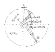
Figure 15: Critical curve of source locations.

Fig 15 shows the critical curve for the source locations $x_{s}$ inside the equiangular spiral. That the critical curve itself may again be an equiangular spiral is already suggested by looking at the figure and confirmed by writing 

$$x_{cs} = \mbox{\boldmath$x_{cs0}$}exp((\mathbf{i}+t)\Phi_{s})$$ (67)

$$x_{cs0} = 2sin\delta\,\,\,exp(t\Phi_{0})\,\mbox{\boldmath$x_{0}$}$$

$$\Phi_{0} = \frac{3}{2}\pi+\delta\mbox{ for }0\leq\Phi_{s}<\frac{\pi}{2}-\delta$$

$$\mbox{ and }\,\,\,\,-\frac{\pi}{2}+\delta\mbox{ otherwise.}$$

This mere fact lends itself to the interesting conclusion, that if one would ”physically” place an equiangular spiral at the location of the critical equiangular spiral (curve) described by eq. (67) inside the original equiangular spiral given by eq. (6), all light rays emitted from the gap of this critical equiangular spiral would naturally be only right side incident rays for points of incidence on the orignal spiral.

As can be seen from eq. (67) we have $\lim_{\delta\rightarrow 0}\mbox{\boldmath$x_{cs}$}=0$, since $\lim_{\delta\rightarrow 0}sin\delta=0$. This explains the complete absence of any such critical curve in the case of a circle.

Another observation is, that for the special case of $x_{s}=x_{cs}$ eq. (60) can be written as

$$\frac{x_{cs}}{sin2\delta}=\frac{x_{0}exp(t\Phi_{c\pm})}{sin(\Phi_{s}-\Phi_{c\pm}+2\delta)}=\frac{x_{c\pm}}{sin(\Phi_{s}-\Phi_{c\pm}+2\delta)}=\frac{x_{c\pm}}{sin\Psi}$$ (68)

with

$$\Psi=\pi-[(\Phi_{s}-\Phi_{c\pm})+2\delta]=2(\frac{\pi}{2}-\delta)-(\Phi_{s}-\Phi_{c\pm}).$$ (69)

From fig. 15 we see that $\Phi-\Phi_{c\pm}$, $\Psi$ and $2\delta$ are the three angles of the triangle formed by the origin, $x_{cs}$ and $x_{c\pm}$, where each angle and each point correspond to each other as listed. In the case of $\Phi_{s}\geq\frac{\pi}{2}-\delta$ we have $\Phi_{c\pm}=\Phi_{s}+\delta-\frac{\pi}{2}$, hence

$$\Phi_{s}-\Phi_{c\pm}=\Phi_{s}-\Phi_{s}-\delta+\frac{\pi}{2}=\frac{\pi}{2}-\delta$$ (70)

We therefore obtain according to (69):

$$\Psi=\frac{\pi}{2}-\delta=\Phi_{s}-\Phi_{c\pm}$$ (71)

This shows that the above mentioned triangle is an equilateral triangle with basis lenght $x_{cs}$ and side lenghts $x_{c\pm}$. The same can be shown for $0\leq\Phi_{s}<\frac{\pi}{2}-\delta$.

This in turn can serve as a very simple geometric method in order to construct the critical equiangular spiral. For any $\mbox{\boldmath$x$}(\Phi)$ taken as $\mbox{\boldmath$x_{c\pm}$}(\Phi)$ one rotates the vector $-\mbox{\boldmath$x$}$ attached to $x$ clockwise by $2\delta$ and obtains the corresponding

$$\mbox{\boldmath$x_{cs}$}=\mbox{\boldmath$x$}+(-\mbox{\boldmath$x$})exp(-2\mathbf{i}\delta)=\mbox{\boldmath$x$}(1-exp(-2\mathbf{i}\delta))$$ (72)

Another interesting property of the critical equiangular spiral follows from eq. (67). The $t=tan\delta$ is the same as in the definition of the original equiangular spiral (6). The critical equiangular spiral is therefore just a shrunk (factor: $2sin\delta$) and rotated (anticlockwise by $\frac{\pi}{2}-\delta$) version of the original one.

There is in addition even a way to ”see” the critical equiangular spiral when placing a light ray source at the origin. Because according to eq. (71) the angle $\Psi$ in fig. 15 is exactly $\frac{\pi}{2}-\delta$. Comparing this with eq. (11) we therefore see that the rays reflected at any point $x$(= $x_{c\pm}$) of the original equiangular spiral are precisely tangential to the critical equiangular spiral. The set of one time reflected rays, which originated at the origin represents therefore the set of all tangents to the critical equiangular spiral.

Knowing this and comparing fig. 15 with fig. 12 shows that for $x_{s}(\Phi_{s})>x_{cs}(\Phi_{s})$ the two straight lines through $x_{s}$ and $x_{+}$, and through $x_{s}$ and $x_{-}$ in fig. 12 are actually the two tangents of the critical equiangular spiral through $x_{s}$. This gives a simple geometric construction in order to find the two angular sectors of left- and right incidence for any source $x_{s}$ with the help of the critical equiangular spiral.

4 Conclusion

In this work, I first introduced the way in which geometric calculus describes an equiangular spiral and reflections of light at it. I then discussed the development of a light path through successive reflections. I made a distinction between incidence from the left and from the right relative to the radius vector. It was then found that right incident vectors continue to be right incident, and follow anticlockwise polygonal paths bending closer and closer to the boundary until they eventually leave through the gap.

As for left incident light rays, they first follow clockwise polygonal paths, yet bending further and further away from the boundary until they eventually change their state into right incident rays with anticlockwise polygonal paths.

The conditions of escape and the asymptotic characteristics were analyzed in detail as well.

Finally point sources were placed inside the spiral and the occurence of right- and left incidence, depending on the source location was examined. The very interesting structure of another equiangular sprial, a dilated and rotated concentric version of the original one, was discovered. Rays emitted from any source inside this critical equiangular spiral area were found to be right incident rays at the original equiangular spiral ab initio. The discussion of this critical equiangular spiral was concluded with explaining some of its geometrical and physical properties.

This short treatment of the subject may in itself only be an introduction. Further analysis may still be very fruitful. One may e.g. ask for higher dimensional spirally deformed objects or cavities, like as cones and spheres. Or one may try to impose spiral deformations not only on circles but on other conical sections as well. One may further ask, whether the phenomenon of the self similar second critical equiangular spiral is an artifact of the globally constant $\delta$, or if corresponding structures would exist for $\delta$ being a function of $\Phi$ as well.

The application of numerical techniques may yield a variety of results as well, since in this work I so far have not yet introduced such methods. The transcendental character of the equations will certainly make it necessary for obtaining more quantitative results.

The potential applications of this sort of analysis should be very wide, including the fields of optics, electromagnetic waves in general as well as acoustics.

In optics, it may lead amongst other possible applications, to the development of new types of laser resonators and to logical components for optical computing . New types of telescopes may arise as well from further analyzing image propagation (i.e. ensembles of light rays defining images).

For electromagnetic waves in general, new types of resonators and antennas may result.

As for acoustics, architects might find it interesting to construct spirally shaped buildings, instead of circular ones in order to conduct the sound in certain directions.

5 Acknowledgements

I first of all want to thank God, my creator, who allowed me to enjoy this interesting piece of research [5] in the first place. An ancient biblical acrostic poem declares: ”Great are the works of the Lord; They are pondered by all who delight in them. … The fear of the Lord is the beginning of wisdom; all who follow his precepts have good understanding. To him belongs eternal praise.” I am indebted to K. Shinoda, who always encouraged me and prayed for me during this research. I further thank J.S.R. Chisholm, who greatly stirred my interest in geometric calculus. Discussions with H. Ishi at the university of Kyoto proved very helpful for advancing the ideas presented. I finally thank the university of Fukui for providing the environment for carrying out this research work.

References

- [1] David Hestenes, Garret Sobczyk. Clifford Algebra to Geometric Calculus, A Unified Language for Mathematics and Physics. D. Reidel Pub. Comp., Dordrecht, 1984.
- [2] Otis Port (ed.). Laser Flashes - Follow The Bouncing Light. Business Week, Asian Edition, June 15:73, 1998.
- [3] David Hestenes. New Foundations for Classical Mechanics. D. Reidel Pub. Comp., Dordrecht, 1987.
- [4] Jens U. Nöckel. Mikrolaser als Photonen-Billards: wie Chaos ans Licht kommt. Physikalische Blätter, 54:927, 1998.
- [5] International Bible Society and BibleGateway. Bible, New International Version, Psalm 111, verses 2 and 10. IBS, Colorado, 1984. http://bible.gospelcom.net/.