Error control of a numerical formula for the Fourier transform by Ooura’s continuous Euler transform and fractional FFT

Ken’ichiro Tanaka ketanaka@fun.ac.jp School of Systems Information Science, Future University Hakodate,
116-2 Kamedanakano-cho, Hakodate, Hokkaido, 041-8655, Japan
Abstract

In this paper, we consider a method for fast numerical computation of the Fourier transform of a slowly decaying function with given accuracy in given ranges of the frequency. In these decades, some useful formulas for the Fourier transform are proposed to recover difficulty of the computation due to the slow decay and the oscillation of the integrand. In particular, Ooura proposed formulas with continuous Euler transformation and showed their effectiveness. It is, however, also reported that errors of them become large outside some ranges of the frequency. Then, for an illustrating representative of the formulas, we choose parameters in the formula based on its error analysis to compute the Fourier transform with given accuracy in given ranges of the frequency. Furthermore, combining the formula and fractional FFT, a generalization of the fast Fourier transform (FFT), we execute the computation in the same order of computation time as the FFT.

keywords:
error control , Fourier transform , continuous Euler transform , fractional FFT

1 Introduction

In this paper, we consider a method for fast numerical computation of the Fourier transform

$\displaystyle F(\omega)=\int_{-\infty}^{\infty}f(x)\,\mathrm{e}^{-\mathrm{i}\,\omega\,x}\,\mathrm{d}x$ (1.1)

with given accuracy in given ranges of the frequency $\omega$. In particular, we mainly focus on a function $f(x)$ in (1.1) with slow decay as $x\to\pm\infty$. The Fourier transform is a fundamental tool in various areas such as optics, signal processing, probability theory, and theoretical or numerical methods for differential equations [1], etc. Moreover, in mathematical finance, option pricing by the Fourier transform is an active research topic [2]. Particularly in this area, fast numerical computation of the Fourier transform is required. On the other hand, it is usually needed to compute the values of $F(\omega)$ in (1.1) for many $\omega$’s in some ranges. Then, it is preferable to use some methods to accelerate the computation such as the fast Fourier transform (FFT).

Since the Fourier transform (1.1) is a definite integral for fixed $\omega$, we may apply some standard quadrature formulas to (1.1) such as Newton-Cotes type or Gauss type formulas. These formulas can yield accurate approximate values for $F(\omega)$ if the function $f(x)$ in (1.1) is sufficiently smooth and decays rapidly as $x\to\pm\infty$. For $f$ with slow decay, however, less accurate values are generated by these formulas. Moreover, we may also use double exponential (DE) formulas by Takahasi and Mori [3] for the computation. The DE formulas are formed by some special variable transformations $\phi$ as

$\displaystyle\int g(x)\,\mathrm{d}x\approx h\sum_{n=-N_{-}}^{N_{+}}g(\phi(nh))\,\phi^{\prime}(nh)$ (1.2)

for a function $g$, where $h>0$ is a width between sampling points. The transformations $\phi$ are called double exponential (DE) transformations. The DE formulas are very accurate for a reasonably wide class of definite integrals [4]. It is, however, known that the DE formulas do not yield so accurate results for oscillatory integrals such as (1.1) with slowly decaying $f$.

Several highly accurate formulas for the Fourier transform of slowly decaying functions are proposed by Ooura and Mori [5][6] and Ooura [7]. In [5][6], DE formulas specialized for oscillatory integrals are proposed. In these formulas, parameters such as $h$ in (1.2) etc. depend on the frequency $\omega$. Then, to compute $F(\omega)$ for another $\omega$, we need to change the parameters in these formulas. In [7], another DE formula is proposed to compute $F(\omega)$ for a certain range of $\omega$ with constant parameters in the formula. This formula, however, has some restriction for the setting of the range, and direct application of the FFT to the formula is not straightforward. On the other hand, Ooura [8][9] proposed other useful formulas

$\displaystyle F(\omega)$ $\displaystyle\approx h\sum_{n=-N_{-}}^{N_{+}}w(|nh|)\,f(nh)\,\mathrm{e}^{-\mathrm{i}\,\omega\,nh},$ (1.3)

using continuous Euler transformations $w$ with some parameters. Accuracy of these formulas and applicability of the FFT to them are already shown. It is, however, also reported that errors of them become large for $\omega$ with large $|\omega|$ or for $\omega$ around points of discontinuity of $F$ when $h$ and the parameters in $w$ are independent of $\omega$.

In this paper, we focus on the formula (1.3) in [8] with $w$ defined by (2.1) later. Then, based on error analysis of the formula, we find appropriate setting of the parameters in it to compute the Fourier transform $F(\omega)$ with given accuracy in given ranges of the frequency $\omega$. Furthermore, combining the formula and fractional FFT, a generalization of the FFT, we show that the computation can be done in the same order of computation time as the FFT.

The rest of this paper is organized as follows. In Section 2, we describe the formula with the continuous Euler transform. In Section 3, we investigate error of the formula, show appropriate setting of the parameters, and present an error bound of the formula under the setting. In Section 4, we explain the fractional FFT and show some numerical examples. Proofs of lemmas for the error analysis are shown in Section 5. Finally, we conclude this paper by Section 6.

2 Numerical formula by Ooura’s continuous Euler transform

Let $w(x;p,q)$ be defined by

$\displaystyle w(x;p,q)=\frac{1}{2}\mathop{\mathrm{erfc}}\left(\frac{x}{p}-q\right),$ (2.1)

where

$\displaystyle\mathop{\mathrm{erfc}}(x)=\frac{2}{\sqrt{\pi}}\int_{x}^{\infty}\exp(-t^{2})\,\mathrm{d}t.$ (2.2)

Ooura [8] introduced a continuous Euler transform of $F$ in (1.1) defined by

$\displaystyle F_{w}(\omega)=\int_{-\infty}^{\infty}w(|x|;p,q)f(x)\,\mathrm{e}^{-\mathrm{i}\,\omega\,x}\mathrm{d}x.$ (2.3)

As shown later by Lemma 1, this function $F_{w}$ approximates $F$ on some assumptions. Then, applying the trapezoidal formula to the integral in (2.3) yields a numerical formula:

$\displaystyle F(\omega)$ $\displaystyle\approx h\sum_{n=-N-1}^{N}w(|nh|;p,q)f(nh)\,\mathrm{e}^{-\mathrm{i}\,\omega\,nh},$ (2.4)

where $h$ is a positive real number and $N$ is a positive integer. Using the approximation (2.4), we can numerically obtain the function $F$ on a given interval $[-\omega_{u},\omega_{u}]\ (\omega_{u}>0)$. Namely, setting

$\displaystyle\tilde{h}=\omega_{u}/(N+1),$ (2.5)

we may compute the RHS of (2.4) for $\omega=-(N+1)\,\tilde{h},\ldots,N\tilde{h}$, i.e.,

$\displaystyle h\sum_{n=-N-1}^{N}w(|nh|;p,q)f(nh)\,\mathrm{e}^{-\mathrm{i}\,mnh\tilde{h}}\qquad(m=-N-1,\ldots,N).$ (2.6)

To compute the values (2.6) with given accuracy, we need to choose the parameters $p$, $q$, $h$ and $N$ appropriately. We give such choice of them in Section 3.

3 Error control of the numerical formula

3.1 Error estimate

We begin with error estimate of the approximation (2.4) to find appropriate choice of the parameters $p$, $q$, $h$ and $N$. Here, we introduce the following notations:

$\displaystyle F_{w}^{(\infty,h)}(\omega)$ $\displaystyle=h\sum_{n=-\infty}^{\infty}w(|nh|;p,q)f(nh)\,\mathrm{e}^{-\mathrm{i}\,\omega\,nh},$ (3.1)
$\displaystyle F_{w}^{(N,h)}(\omega)$ $\displaystyle=h\sum_{n=-N-1}^{N}w(|nh|;p,q)f(nh)\,\mathrm{e}^{-\mathrm{i}\,\omega\,nh}.$ (3.2)

Then, the error $|F(\omega)-F_{w}^{(N,h)}(\omega)|$ can be bounded as follows:

$\displaystyle|F(\omega)-F_{w}^{(N,h)}(\omega)|\leq E_{w}(\omega)+E_{w}^{(\infty,h)}(\omega)+E_{w}^{(N,h)}(\omega),$ (3.3)

where

$\displaystyle E_{w}(\omega)$ $\displaystyle=|F(\omega)-F_{w}(\omega)|,$ (3.4)
$\displaystyle E_{w}^{(\infty,h)}(\omega)$ $\displaystyle=|F_{w}(\omega)-F_{w}^{(\infty,h)}(\omega)|,$ (3.5)
$\displaystyle E_{w}^{(N,h)}(\omega)$ $\displaystyle=|F_{w}^{(\infty,h)}(\omega)-F_{w}^{(N,h)}(\omega)|.$ (3.6)

To estimate these errors, we consider the domains

$\displaystyle\mathcal{T}_{\alpha}$ $\displaystyle=\{z\in\mathbf{C}\mid|\mathrm{arg}\,z|<\mathop{\mathrm{arctan}}\alpha\text{ or }|\pi-\mathrm{arg}\,z|<\mathop{\mathrm{arctan}}\alpha\},$ (3.7)
$\displaystyle\mathcal{D}_{d}$ $\displaystyle=\{z\in\mathbf{C}\mid|\mathrm{Im}\,z|<d\}$ (3.8)

for $0<\alpha<1$ and $d>0$, and the following assumptions for $f$:

Assumption 1.

The function $f$ is analytic on $\mathcal{T}_{\alpha}$, $|f(z)|\leq M$ for any $z\in\mathcal{T}_{\alpha}$, and

$\displaystyle\lim_{R\to\infty}\max_{-\alpha\leq\beta\leq\alpha}\left|f(\pm R+\mathrm{i}\,\beta\,R)\right|=0.$ (3.9)
Assumption 2.

The function $f$ is analytic on $\mathcal{D}_{d}$, $|f(z)|\leq M$ for any $z\in\mathcal{D}_{d}$, and belongs to $L^{2}(\mathbf{R})$, i.e., $f$ is square integrable on $\mathbf{R}$.

First, an estimate of $E_{w}(\omega)$ is given by Lemma 1 below. We omit the proof of this lemma because it can be shown in the same manner as Ooura [8, Theorem 2].

Lemma 1.

On Assumption 1, for arbitrary $\alpha^{\prime}$ with $0<\alpha^{\prime}\leq\alpha$, we have

$\displaystyle E_{w}(\omega)\leq M\sqrt{1+\alpha^{\prime 2}}\left[\frac{\sqrt{\pi}p}{\sqrt{1-\alpha^{\prime 2}}}\exp\left[-q^{2}\left\{1-\left(\frac{\alpha^{\prime}p}{2q}|\omega|-1\right)^{2}/(1-\alpha^{\prime 2})\right\}\right]+\frac{2}{\omega\alpha^{\prime}}\,\mathrm{e}^{-|\omega|\,\alpha^{\prime}\,p\,q}\right].$ (3.10)

Next, estimates of $E_{w}^{(\infty,h)}(\omega)$ and $E_{w}^{(N,h)}(\omega)$ are given by Lemmas 2 and 3 below, respectively. Proofs of them are presented in Section 5.

Lemma 2.

On Assumption 2, for $\omega$ with $|\omega|\leq\pi/h$, we have

$\displaystyle E_{w}^{(\infty,h)}(\omega)\leq\frac{2\,C_{M,p,q,d}}{1-\exp(-2\,\pi\,d/h)}\exp\left(-\frac{\pi\,d}{h}\right),$ (3.11)

where

$\displaystyle C_{M,p,q,d}=M\left(\frac{\sqrt{\pi}}{2}+q\right)\,p\,\exp\{(d/p)^{2}\}.$ (3.12)
Lemma 3.

On Assumption 2 and under the condition $Nh>pq$, we have

$\displaystyle E_{w}^{(N,h)}(\omega)$ $\displaystyle\leq\frac{\sqrt{\pi}\,p\,M}{2}\,\exp\left\{-\frac{(Nh-pq)^{2}}{p^{2}}\right\}.$ (3.13)
Remark 1.

Lemmas 2 and 3 are important because they give explicit error bounds, although they are standard estimates of the discretization error and the truncation error of the trapezoidal formula for the function $w(|x|;p,q)f(x)\,\mathrm{e}^{-\mathrm{i}\,\omega\,x}$, respectively. As a technical note, we point out that the function $w(|z|;p,q)$ is not an analytic function of $z$ in $\mathcal{D}_{d}$. Then, we apply a smoothing technique to $w(|z|;p,q)$ to prove Lemma 2 as shown in Section 5.

Remark 2.

It is possible to use another weight function $\tilde{w}(z;\tilde{p},\tilde{q})$ analytic in $\mathcal{D}_{d}$ which realizes a similar formula to (2.4). In this paper, however, we analyze the formula (2.4) to show theoretically that even the non-smooth function $w(|z|;p,q)$ can achieve the exponential convergence rate shown in Lemma 2.

3.2 Choice of parameters and error control

Using Lemmas 1, 2 and 3, we show in Theorem 4 below that appropriate choice of the parameters enables the formula (2.4) to compute the Fourier transform $F(\omega)$ with given accuracy in given ranges of $\omega$.

Theorem 4.

Let Assumptions 1 and 2 be satisfied. Let $\omega_{d}$ and $\omega_{u}$ be real numbers with $0<\omega_{d}<\omega_{u}$ and $\omega_{d}/\omega_{u}\leq\min\{\alpha,1/2\}$, let $N$ be an integer with

$\displaystyle N\geq\frac{2\,d\,(\omega_{d}+\omega_{u})\,\omega_{u}^{2}}{\pi\,\omega_{d}^{2}},$ (3.14)

and let $h$, $p$, $q$ be defined by

$\displaystyle h=\sqrt{\frac{2\,\pi\,d\,(\omega_{d}+\omega_{u})}{\omega_{d}^{2}\,N}},\quad p=\sqrt{\frac{N\,h}{\omega_{d}}},\quad q=\sqrt{\frac{\omega_{d}\,N\,h}{4}}.$ (3.15)

Then, for any $\omega$ with $\omega_{d}\leq|\omega|\leq\omega_{u}$, we have

$\displaystyle\left|F(\omega)-F_{w}^{(N,h)}(\omega)\right|\leq C(N)\,\exp\left(-\sqrt{\frac{\pi\,d\,\omega_{d}^{2}\,N}{2\,(\omega_{d}+\omega_{u})}}\right),$ (3.16)

where $C(N)=C_{1}(N)+C_{2}(N)+C_{3}(N)$ and

$\displaystyle C_{1}(N)$ $\displaystyle=M\sqrt{\omega_{u}^{2}+\omega_{d}^{2}}\left\{\frac{\sqrt{\pi}}{\sqrt{\omega_{u}^{2}-\omega_{d}^{2}}}\left(\frac{2\,\pi\,d\,(\omega_{d}+\omega_{u})\,N}{\omega_{d}^{4}}\right)^{1/4}+\frac{2}{\omega_{d}^{2}}\right\},$ (3.17)
$\displaystyle C_{2}(N)$ $\displaystyle=\frac{2\,M}{1-\mathrm{e}^{-2\,d\,\omega_{u}}}\left\{\frac{\sqrt{\pi}}{2}\left(\frac{2\,\pi\,d\,(\omega_{d}+\omega_{u})\,N}{\omega_{d}^{4}}\right)^{1/4}+\sqrt{\frac{\pi\,d\,(\omega_{d}+\omega_{u})N}{2\,\omega_{d}^{2}}}\right\}\,\mathrm{e}^{d\,\omega_{d}/4},$ (3.18)
$\displaystyle C_{3}(N)$ $\displaystyle=\frac{\sqrt{\pi}\,M}{2}\left(\frac{2\,\pi\,d\,(\omega_{d}+\omega_{u})\,N}{\omega_{d}^{4}}\right)^{1/4}.$ (3.19)
Remark 3.

Since Assumption 2 does not exclude the case $f\not\in L^{1}(\mathbf{R})$, the Fourier transform $F$ may be discontinuous at $\omega=0$. Then, we consider the positive lower bound $\omega_{d}$ of $|\omega|$ in Theorem 4.

Remark 4.

It follows from the estimate (3.16) that $|F(\omega)-F_{w}^{(N,h)}(\omega)|=\mathrm{O}(\sqrt{N}\,\exp(-c\sqrt{N}))$ for a constant $c>0$ independent of $N$. Therefore, appropriate setting of $N$ realizes any given accuracy of the formula.

Proof of Theorem 4.

Using the parameters in (3.15), we estimate the error bounds in Lemmas 1, 2, and 3. First, setting $\alpha^{\prime}=\omega_{d}/\omega_{u}$ in (3.10) of Lemma 1 and noting $\omega_{d}\leq|\omega|\leq\omega_{u}$, we have

$\displaystyle 1-\left(\frac{\alpha^{\prime}p}{2q}|\omega|-1\right)^{2}/(1-\alpha^{\prime 2})$ $\displaystyle=1-\frac{(|\omega|/\omega_{u}-1)^{2}}{1-(\omega_{d}/\omega_{u})^{2}}\geq 1-\frac{(\omega_{d}/\omega_{u}-1)^{2}}{1-(\omega_{d}/\omega_{u})^{2}}=\frac{2\,\omega_{d}/\omega_{u}}{1+\omega_{d}/\omega_{u}}.$ (3.20)

Therefore we have

$\displaystyle q^{2}\left\{1-\left(\frac{\alpha^{\prime}p}{2q}|\omega|-1\right)^{2}/(1-\alpha^{\prime 2})\right\}\geq\frac{\omega_{d}^{2}\,N\,h}{2\,(\omega_{d}+\omega_{u})}.$ (3.21)

Moreover, as for the last term in (3.10), we can deduce

$\displaystyle|\omega|\,\alpha^{\prime}\,p\,q\geq\frac{\omega_{d}^{2}\,N\,h}{2\,\omega_{u}}.$ (3.22)

Then, combining (3.10), (3.21) and (3.22), we have

$\displaystyle E_{w}(\omega)$ $\displaystyle\leq M\sqrt{1+(\omega_{d}/\omega_{u})^{2}}\left\{\frac{\sqrt{\pi}}{\sqrt{1-(\omega_{d}/\omega_{u})^{2}}}\sqrt{\frac{N\,h}{\omega_{d}}}+\frac{2\,\omega_{u}}{\omega_{d}^{2}}\right\}\,\exp\left(-\frac{\omega_{d}^{2}\,N\,h}{2\,(\omega_{d}+\omega_{u})}\right)$
$\displaystyle=C_{1}(N)\,\exp\left(-\sqrt{\frac{\pi\,d\,\omega_{d}^{2}\,N}{2\,(\omega_{d}+\omega_{u})}}\right).$ (3.23)

Next, to use Lemma 2 to estimate $E_{w}^{(\infty,h)}(\omega)$, we need to check $\omega_{u}\leq\pi/h$. This follows from (3.14) and the definition of $h$ in (3.15). Then, substituting $h,p,q$ in (3.15) into (3.11) and (3.12), we have

$\displaystyle E_{w}^{(\infty,h)}(\omega)\leq C_{2}(N)\,\exp\left(-\sqrt{\frac{\pi\,d\,\omega_{d}^{2}\,N}{2\,(\omega_{d}+\omega_{u})}}\right).$ (3.24)

Finally, substituting $h,p,q$ in (3.15) into (3.13) and noting $\omega_{d}/\omega_{u}\leq 1/2$, we have

$\displaystyle E_{w}^{(N,h)}(\omega)$ $\displaystyle\leq C_{3}(N)\,\exp\left(-\frac{\omega_{d}\,N\,h}{4}\right)\leq C_{3}(N)\,\exp\left(-\frac{\omega_{d}^{2}\,N\,h}{2\,(\omega_{d}+\omega_{u})}\right)$
$\displaystyle=C_{3}(N)\,\exp\left(-\sqrt{\frac{\pi\,d\,\omega_{d}^{2}\,N}{2\,(\omega_{d}+\omega_{u})}}\right).$ (3.25)

From the estimates (3.23), (3.24) and (3.25), we obtain the conclusion. ∎

4 Numerical Experiments

Recall that we need to compute the values

$\displaystyle F_{w}^{(N,h)}(m\tilde{h})$ $\displaystyle=h\sum_{n=-N-1}^{N}w(|nh|;p,q)f(nh)\,\mathrm{e}^{-\mathrm{i}\,mnh\tilde{h}}$ (4.1)

for $m=-N-1,\ldots,N$, where $\tilde{h}$ is defined by (2.5) and $h$, $p$, $q$ are defined by (3.15), respectively. Unless $\tilde{h}$ and $h$ satisfy $h\tilde{h}=\pi/(N+1)$, we cannot use the FFT directly to the computation of (4.1). Then, we use fractional FFT described in Section 4.1 below, and show some numerical examples in Section 4.2.

4.1 Fractional FFT

Fractional FFT is developed by Bailey and Swarztrauber [10] to enable computation of a sum such as (4.1) with arbitrary $h$ and $\tilde{h}$. For example, Chourdakis [11] applied the fractional FFT to option pricing problems.

The fractional FFT is derived by regarding the sum in (4.1) as a circular convolution. For simplicity, we introduce $m^{\prime}=m+N+1$ and $n^{\prime}=n+N+1$ to shift the range of the indexes as follows:

$\displaystyle F_{w}^{(N,h)}(m\tilde{h})$ $\displaystyle=h\sum_{n^{\prime}=0}^{2(N+1)-1}w(|(n^{\prime}-N-1)h|;p,q)f((n^{\prime}-N-1)h)\,\mathrm{e}^{-\mathrm{i}\,(m^{\prime}-N-1)(n^{\prime}-N-1)h\tilde{h}}$
$\displaystyle=\mathrm{e}^{\mathrm{i}\,(m^{\prime}-N-1)(N+1)h\tilde{h}}\sum_{n^{\prime}=0}^{2(N+1)-1}x_{n^{\prime}}\,\mathrm{e}^{-\mathrm{i}\,m^{\prime}n^{\prime}h\tilde{h}},$ (4.2)

where $x_{n^{\prime}}=h\,w(|(n^{\prime}-N-1)h|;p,q)f((n^{\prime}-N-1)h)\,\mathrm{e}^{\mathrm{i}\,(N+1)\,n^{\prime}\,h\tilde{h}}$. Then, for $m^{\prime}=0,\ldots,2(N+1)$, the sum in (4.2) is rewritten in the form

$\displaystyle\sum_{n^{\prime}=0}^{2(N+1)-1}x_{n^{\prime}}\,\mathrm{e}^{-\mathrm{i}\,m^{\prime}n^{\prime}h\tilde{h}}=\sum_{n^{\prime}=0}^{2(N+1)-1}x_{n^{\prime}}\,\mathrm{e}^{-\pi\mathrm{i}\,\{m^{\prime 2}+n^{\prime 2}-(m^{\prime}-n^{\prime})^{2}\}\alpha}=\mathrm{e}^{-\pi\mathrm{i}\,m^{\prime 2}\alpha}\sum_{n^{\prime}=0}^{2(N+1)-1}y_{n^{\prime}}\,z_{m^{\prime}-n^{\prime}},$ (4.3)

where $\alpha=h\tilde{h}/(2\pi)$, $y_{n^{\prime}}=x_{n^{\prime}}\,\mathrm{e}^{-\pi\mathrm{i}\,n^{\prime 2}\alpha}$ and $z_{n^{\prime}}=\mathrm{e}^{\pi\mathrm{i}\,n^{\prime 2}\alpha}$. Note that the sum in (4.3) is a convolution but not circular, i.e., we cannot regard $\{z_{n^{\prime}}\}_{n^{\prime}=0}^{2N+1}$ as $2(N+1)$-periodic such as $z_{n^{\prime}+2(N+1)}=z_{n^{\prime}}$. Then, we need to convert this sum into a form of a circular convolution. A way for this conversion is to extend $\{y_{n^{\prime}}\}_{n^{\prime}=0}^{2N+1}$ and $\{z_{n^{\prime}}\}_{n^{\prime}=0}^{2N+1}$ to length $4(N+1)$ by setting

$\displaystyle y_{n^{\prime}}=0,\quad z_{n^{\prime}}=\mathrm{e}^{\pi\mathrm{i}\,\{4(N+1)-n^{\prime}\}^{2}\alpha}$ (4.4)

for $n^{\prime}$ with $2(N+1)\leq n^{\prime}<4(N+1)$. Then, combining (4.2), (4.3) and (4.4), we have an expression of $F_{w}^{(N,h)}(m\tilde{h})$ with a circular convolution:

$\displaystyle F_{w}^{(N,h)}(m\tilde{h})=e_{m^{\prime}}\sum_{n^{\prime}=0}^{4(N+1)-1}y_{n^{\prime}}\,z_{m^{\prime}-n^{\prime}},$ (4.5)

where $e_{m^{\prime}}=\mathrm{e}^{2\pi\mathrm{i}\,(m^{\prime}-N-1)(N+1)\alpha-\pi\mathrm{i}\,m^{\prime 2}\alpha}$. The RHS of (4.5) can be obtained by

$\displaystyle\{e_{m^{\prime}}\}\odot\left\{\mathrm{IDFT}_{m^{\prime}}\left(\,\{\mathrm{DFT}_{\ell^{\prime}}(\{y_{n^{\prime}}\})\}\odot\{\mathrm{DFT}_{\ell^{\prime}}(\{z_{n^{\prime}}\})\}\,\right)\right\},$ (4.6)

where $\odot$ denotes element-by-element vector multiplication, and $\mathrm{DFT}$ and $\mathrm{IDFT}$ denote the discrete and inverse discrete Fourier transform, respectively. Therefore, applying the ordinal FFT to $\mathrm{DFT}$ and $\mathrm{IDFT}$ in (4.6), we can compute (4.5) with computation time $\mathrm{O}(N\log N)$.

4.2 Numerical Examples

We consider the following functions $f_{i}$ and their Fourier transforms $F_{i}$.

Example 1.
$\displaystyle f_{1}(x)=\frac{1}{\sqrt{1+x^{2}}},\quad F_{1}(\omega)=2\,K_{0}(|\omega|).$ (4.7)
Example 2.
$\displaystyle f_{2}(x)=\frac{1}{(1-\mathrm{i}\,x)^{2}},\quad F_{2}(\omega)=\begin{cases}0&(\omega<0),\\ 2\pi\,\omega\,\mathrm{e}^{-\omega}&(\omega\geq 0).\end{cases}$ (4.8)

The function $f_{1}$ is taken from [8], where $K_{0}$ is the modified Bessel function of the second kind. The function $f_{2}$ is the characteristic function of the gamma distribution $\mathrm{Ga}(2,1)$, and $F_{2}(\omega)/(2\pi)$ is the density function of $\mathrm{Ga}(2,1)$. The functions $f_{1}$ and $f_{2}$ satisfy $f_{1}(x)=\mathrm{O}(|x|^{-1})\ (x\to\pm\infty)$ and $f_{2}(x)=\mathrm{O}(|x|^{-2})\ (x\to\pm\infty)$, respectively. Moreover, $F_{1}$ is discontinuous at $\omega=0$, and $F_{2}$ is not differentiable at $\omega=0$.

To use Theorem 4, we note that $f_{1}$ satisfies Assumptions 1 and 2 for

$\displaystyle\alpha=d=1-\varepsilon_{1},\ M=1/\sqrt{\varepsilon_{1}},$ (4.9)

and $f_{2}$ satisfies them for

$\displaystyle\alpha=d=1-\varepsilon_{2},\ M=\max\{2,\,1/\varepsilon_{2}^{2}\},$ (4.10)

where $\varepsilon_{i}\ (i=1,2)$ are arbitrary real numbers with $0<\varepsilon_{i}<1\ (i=1,2)$. Here, we use $\varepsilon_{1}=0.01$ and $\varepsilon_{2}=0.1$. Using these, we apply the formula (4.1) to $f_{i}\ (i=1,2)$ in the following procedure.

  1. 1.

    Give $\omega_{d}$ and $\omega_{u}$ in Theorem 4, and set an error bound $\epsilon$ by which errors of the computed values for $\omega=m\tilde{h}$ with $\omega_{d}\leq|\omega|\leq\omega_{u}$ should be bounded.

  2. 2.

    Choose $N$ from $\{2^{j}-1\mid j=1,2,\ldots\}$ satisfying (3.14) and (The RHS of (3.16))ϵ(The RHS of (3.16))italic-ϵ\text{(The RHS of \eqref{eq:MainEstim})}\leq\epsilon. Let $N_{\epsilon}$ denote $N$ chosen here.

  3. 3.

    Set $h$, $p$ and $q$ by (3.15), and apply the formula (4.1) to $f_{i}\ (i=1,2)$ with the fractional FFT.

For this experiment, we choose the following sets of $\omega_{d}$, $\omega_{u}$ and $\epsilon$.

$\displaystyle\text{(A)}\ \omega_{d}=2,\omega_{u}=10,\quad\text{(B)}\ \omega_{d}=1,\omega_{u}=10,\quad\text{(C)}\ \omega_{d}=1.25,\omega_{u}=15,$ (4.11)
$\displaystyle\text{(a)}\ \epsilon=10^{-3},\quad\text{(b)}\ \epsilon=10^{-6}.$ (4.12)

Then, we compute (4.1) for the six combinations of (4.11) and (4.12) for $f_{i}\ (i=1,2)$.

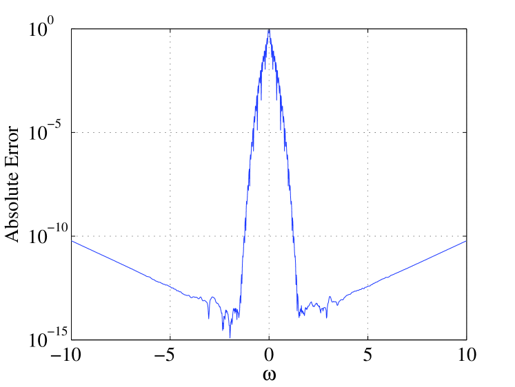
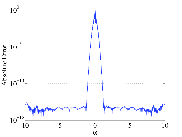
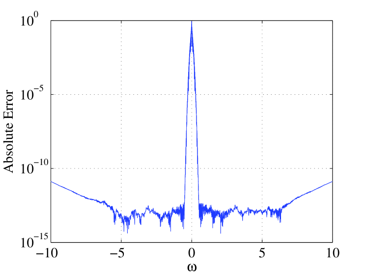
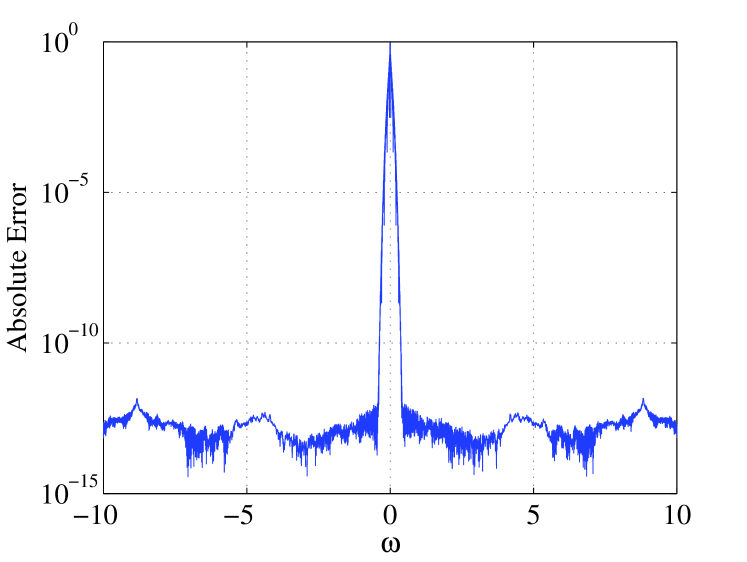
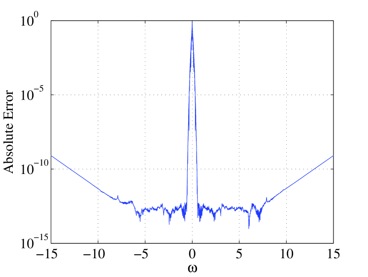
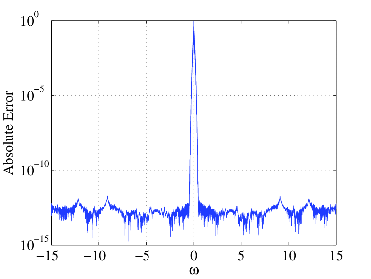
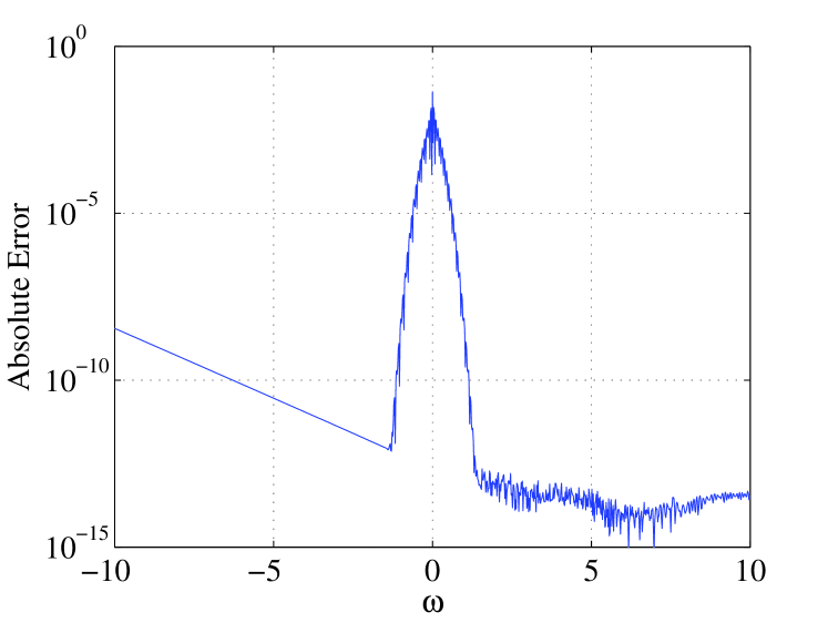
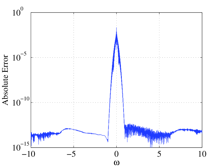
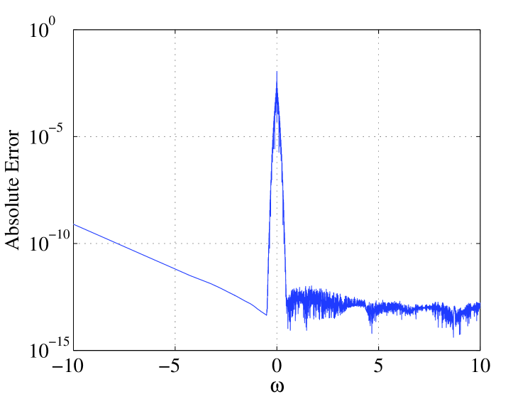
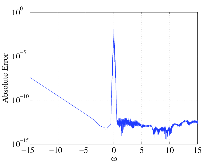
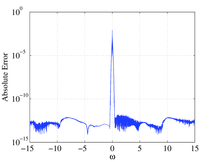
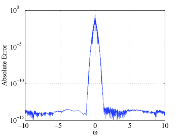
All computations are done by MATLAB R2013a programs with double precision floating point arithmetic on a PC with 3.0GHz CPU and 2GB RAM. The integers $N_{\epsilon}$ and computation times in the all cases are shown by Table 1 for Example 1 and Table 2 for Example 2. Each computation time is a mean of three results measured by three executions of each case. These results show that the computation time is about doubled when $N_{\epsilon}$ increases about by two times, which is about in accordance with the order of the theoretical time $\mathrm{O}(N\log N)$. Furthermore, errors of these computations are shown by Figures 66 for Example 1 and Figures 1212 for Example 2, respectively. Then, we can observe that these results are consistent with the theoretical estimate of Theorem 4, although it does not seem to be tight because the real errors are much smaller than the bounds given in (4.12).

Here, using Example 2, we show another application of the formula (4.1). Let $G_{2}$ denote the indefinite integral of $F_{2}(\omega)/(2\pi)$:

$\displaystyle G_{2}(\omega)=\frac{1}{2\pi}\int_{-\infty}^{\omega}F_{2}(\nu)\,\mathrm{d}\nu=\begin{cases}0&(\omega<0),\\ 1-(1+\omega)\,\mathrm{e}^{-\omega}&(\omega\geq 0).\end{cases}$ (4.13)

This is the cumulative distribution function of the Gamma distribution $\mathrm{Ga}(2,1)$. We show that $G_{2}$ can be computed directly from the characteristic function $f_{2}$ in (4.8) by the formula (4.1). Since $G_{2}$ does not have the inverse Fourier transform, using the Heaviside function

$\displaystyle H(\omega)=\begin{cases}0&(\omega<0),\\ 1&(\omega\geq 0),\end{cases}$ (4.14)

we define a function $\tilde{G}_{2}$ by

$\displaystyle\tilde{G}_{2}(\omega)=G_{2}(\omega)-H(\omega)$ (4.15)

such that $\tilde{G}_{2}$ has the inverse Fourier transform $\tilde{f}_{2}$:

$\displaystyle\tilde{f}_{2}(x)=\frac{1}{2\pi}\int_{-\infty}^{\infty}\tilde{G}_{2}(\omega)\,\mathrm{e}^{\mathrm{i}\,x\,\omega}\,\mathrm{d}\omega=\begin{cases}\displaystyle\mathrm{i}\,\frac{f_{2}(x)-1}{2\pi x}&(x\neq 0),\\ \mathrm{i}\,f^{\prime}_{2}(0)/(2\pi)&(x=0).\end{cases}$ (4.16)

The function $\tilde{f}_{2}$ satisfies Assumptions 1 and 2 for

$\displaystyle\alpha=d=1-\tilde{\varepsilon}_{2},\,M=\max\{2\sqrt{2}/\pi,3/(2\pi\tilde{\varepsilon}_{2}^{2})\},$ (4.17)

where $\tilde{\varepsilon}_{2}$ is an arbitrary real number with $0<\tilde{\varepsilon}_{2}<1$. Then, using the formula (4.1), we can obtain approximate values of $G_{2}(m\tilde{h})\ (m=-N-1,\ldots,N)$ as follows:

$\displaystyle G_{2}(m\tilde{h})\approx h\sum_{n=-N-1}^{N}w(|nh|;p,q)\tilde{f}_{2}(nh)\,\mathrm{e}^{-\mathrm{i}\,mnh\tilde{h}}+H(m\tilde{h}).$ (4.18)

Here, we show the result in the case of (A)-(a) in (4.11) and (4.12). The other cases can be done similarly. For $\tilde{\varepsilon}_{2}=0.1$ in (4.17) we choose $N_{\epsilon}=1023$ and obtain the result shown in Figure 13.

Table 1: The values of $N_{\epsilon}$ determined in the step 2 of the procedure and computation times for Example 1.
$N_{\epsilon}$ Time (sec.)
(A) (a) $511$ $0.039$
(b) $1023$ $0.072$
(B) (a) $2047$ $0.138$
(b) $4095$ $0.271$
(C) (a) $2047$ $0.137$
(b) $4095$ $0.268$
Refer to caption
Figure 1: Error for $F_{1}$ in (4.7) in the case of (A)-(a) in (4.11) and (4.12).
Refer to caption
Figure 2: Error for $F_{1}$ in (4.7) in the case of (A)-(b) in (4.11) and (4.12).
Refer to caption
Figure 3: Error for $F_{1}$ in (4.7) in the case of (B)-(a) in (4.11) and (4.12).
Refer to caption
Figure 4: Error for $F_{1}$ in (4.7) in the case of (B)-(b) in (4.11) and (4.12).
Refer to caption
Figure 5: Error for $F_{1}$ in (4.7) in the case of (C)-(a) in (4.11) and (4.12).
Refer to caption
Figure 6: Error for $F_{1}$ in (4.7) in the case of (C)-(b) in (4.11) and (4.12).
Table 2: The values of $N_{\epsilon}$ determined in the step 2 of the procedure and computation times for Example 2.
$N_{\epsilon}$ Time (sec.)
(A) (a) $511$ $0.040$
(b) $2047$ $0.134$
(B) (a) $2047$ $0.134$
(b) $8191$ $0.507$
(C) (a) $2047$ $0.134$
(b) $4095$ $0.259$
Refer to caption
Figure 7: Error for $F_{2}$ in (4.8) in the case of (A)-(a) in (4.11) and (4.12).
Refer to caption
Figure 8: Error for $F_{2}$ in (4.8) in the case of (A)-(b) in (4.11) and (4.12).
Refer to caption
Figure 9: Error for $F_{2}$ in (4.8) in the case of (B)-(a) in (4.11) and (4.12).
Refer to caption
Figure 10: Error for $F_{2}$ in (4.8) in the case of (B)-(b) in (4.11) and (4.12).
Refer to caption
Figure 11: Error for $F_{2}$ in (4.8) in the case of (C)-(a) in (4.11) and (4.12).
Refer to caption
Figure 12: Error for $F_{2}$ in (4.8) in the case of (C)-(b) in (4.11) and (4.12).
Refer to caption
Figure 13: Error for $G_{2}$ in (4.13) in the case of (A)-(a) in (4.11) and (4.12).

5 Proofs of Lemmas

In this section, we present proofs of Lemmas 2 and 3. We begin with Lemma 3 in Section 5.1 because it is easier. Then, Lemma 2 is proved in Section 5.2 and some other lemmas needed for Lemma 2 are proved in Section 5.3.

5.1 Proof of Lemma 3

Noting

$\displaystyle E_{w}^{(N,h)}(\omega)$ $\displaystyle=\left|h\sum_{n<-N-1,\,N<n}w(|nh|;p,q)f(nh)\,\mathrm{e}^{-\mathrm{i}\,\omega\,nh}\right|$ (5.1)

and $Nh>pq$, we obtain the conclusion of Lemma 3 as follows:

$\displaystyle E_{w}^{(N,h)}(\omega)$ $\displaystyle\leq M\,h\sum_{n>N}|w(|nh|;p,q)|\leq 2\,M\,h\sum_{n=N+1}^{\infty}\frac{1}{2}\exp\left\{-\frac{(nh-pq)^{2}}{p^{2}}\right\}$
$\displaystyle\leq M\,\int_{Nh}^{\infty}\exp\left\{-\frac{(t-pq)^{2}}{p^{2}}\right\}\mathrm{d}t\leq M\,\exp\left\{-\frac{(Nh-pq)^{2}}{p^{2}}\right\}\int_{0}^{\infty}\exp\left\{-\frac{s^{2}}{p^{2}}\right\}\mathrm{d}s$
$\displaystyle=\frac{\sqrt{\pi}\,p\,M}{2}\,\exp\left\{-\frac{(Nh-pq)^{2}}{p^{2}}\right\}.$ (5.2)

5.2 Proof of Lemma 2

For $z\in\mathcal{D}_{d}$, let $w^{\mathrm{sym}}(z;p,q)$ be a function defined by

$\displaystyle w^{\mathrm{sym}}(z;p,q)=\begin{cases}w(z;p,q)&(\mathrm{Re}\,z\geq 0),\\ w(-z;p,q)&(\mathrm{Re}\,z<0).\end{cases}$ (5.3)

Then, $F_{w}^{(\infty,h)}(\omega)$ in (3.1) is rewritten in the form

$\displaystyle F_{w}^{(\infty,h)}(\omega)$ $\displaystyle=h\sum_{n=-\infty}^{\infty}w^{\mathrm{sym}}(nh;p,q)f(nh)\,\mathrm{e}^{-\mathrm{i}\,\omega\,nh}.$ (5.4)

To prove Lemma 2, we use the following fundamental fact.

Lemma 5 (Poisson summation formula [12, Theorem 1.3.1]).

Let $g\in L^{2}(\mathbf{R})$, and let $g$ and its Fourier transform $\hat{g}$ satisfy the conditions

$\displaystyle g(x)$ $\displaystyle=\lim_{t\to+0}\frac{g(x-t)+g(x+t)}{2},$ (5.5)
$\displaystyle\hat{g}(\omega)$ $\displaystyle=\lim_{t\to+0}\frac{\hat{g}(\omega-t)+\hat{g}(\omega+t)}{2}$ (5.6)

for $t$, $x$ and $\omega$ on $\mathbf{R}$. Then, for $\omega$ satisfying (5.6) and $h>0$, the following holds:

$\displaystyle h\sum_{n=-\infty}^{\infty}g(nh)\,\mathrm{e}^{-\mathrm{i}\,\omega\,n\,h}=\sum_{m=-\infty}^{\infty}\hat{g}\left(\frac{2\pi m}{h}-\omega\right).$ (5.7)

A function $g$ defined by $g(z)=w^{\mathrm{sym}}(z;p,q)f(z)$ belongs to $L^{2}(\mathbf{R})$ and continuous on $\mathbf{R}$, and its Fourier transform $\hat{g}$ is continuous on $\mathbf{R}$. Then, we can use Lemma 5 to yield

$\displaystyle F_{w}(\omega)-F_{w}^{(\infty,h)}(\omega)=\hat{g}(\omega)-h\sum_{n=-\infty}^{\infty}g(nh)\,\mathrm{e}^{-\mathrm{i}\,\omega\,n\,h}=-\sum_{m\neq 0}\hat{g}\left(\frac{2\pi m}{h}-\omega\right).$ (5.8)

If the function $\hat{g}$ decays exponentially as $|\hat{g}(\omega)|=\mathrm{O}(\exp(-d\,|\omega|))\ (\omega\to\pm\infty)$, the conclusion of Lemma 2 may follow immediately. The exponential decay of $\hat{g}$, however, is not so straightforwardly shown because $w^{\mathrm{sym}}(z;p,q)$ is not analytic on $\mathcal{D}_{d}$. Then, in the following, we apply smoothing technique to $w^{\mathrm{sym}}(z;p,q)$ to yield an analytic function $g_{\varepsilon}$ approximating $g$, and apply Lemma 5 to $g_{\varepsilon}$.

For sufficiently small $\varepsilon>0$, we define $w^{\mathrm{sym}}_{\varepsilon}(z;p,q)$ by

$\displaystyle w^{\mathrm{sym}}_{\varepsilon}(z;p,q)=\int_{-\infty}^{\infty}u_{\varepsilon}(z-y)\,w^{\mathrm{sym}}(y;p,q)\,\mathrm{d}y,$ (5.9)

where

$\displaystyle u_{\varepsilon}(z)=\frac{1}{\sqrt{2\pi}\,\varepsilon}\exp\left(-\frac{z^{2}}{2\,\varepsilon^{2}}\right),$ (5.10)

and consider $g_{\varepsilon}(z)=w^{\mathrm{sym}}_{\varepsilon}(z;p,q)f(z)$. Using $w^{\mathrm{sym}}_{\varepsilon}(z;p,q)$, we estimate $E_{w}^{(\infty,h)}(\omega)$ as follows:

$\displaystyle E_{w}^{(\infty,h)}(\omega)=|F_{w}(\omega)-F_{w}^{(\infty,h)}(\omega)|\leq E_{w,\varepsilon,\mathrm{int}}^{(\infty,h)}(\omega)+E_{w,\varepsilon,\mathrm{sum}}^{(\infty,h)}(\omega)+E_{w,\varepsilon}^{(\infty,h)}(\omega),$ (5.11)

where

$\displaystyle E_{w,\varepsilon,\mathrm{int}}^{(\infty,h)}(\omega)$ $\displaystyle=\left|\int_{-\infty}^{\infty}(w^{\mathrm{sym}}_{\varepsilon}(x;p,q)-w^{\mathrm{sym}}(x;p,q))\,f(x)\,\mathrm{e}^{-\mathrm{i}\,\omega\,x}\,\mathrm{d}x\right|,$ (5.12)
$\displaystyle E_{w,\varepsilon,\mathrm{sum}}^{(\infty,h)}(\omega)$ $\displaystyle=\left|h\sum_{n=-\infty}^{\infty}(w^{\mathrm{sym}}_{\varepsilon}(nh;p,q)-w^{\mathrm{sym}}(nh;p,q))\,f(nh)\,\mathrm{e}^{-\mathrm{i}\,\omega\,nh}\right|,$ (5.13)
$\displaystyle E_{w,\varepsilon}^{(\infty,h)}(\omega)$ $\displaystyle=\left|\int_{-\infty}^{\infty}w^{\mathrm{sym}}_{\varepsilon}(x;p,q)\,f(x)\,\mathrm{d}x-h\sum_{n=-\infty}^{\infty}w^{\mathrm{sym}}_{\varepsilon}(nh;p,q)f(nh)\,\mathrm{e}^{-\mathrm{i}\,\omega\,nh}\right|.$ (5.14)

To estimate these, we use the following three lemmas, whose proofs are shown in Section 5.3 later.

Lemma 6.

The function $w^{\mathrm{sym}}_{\varepsilon}(z;p,q)$ is analytic on $\mathbf{C}$.

Lemma 7.

The difference $w^{\mathrm{sym}}_{\varepsilon}(z;p,q)-w^{\mathrm{sym}}(z;p,q)$ is absolutely integrable on $\{t\pm d\,\mathrm{i}\mid t\in\mathbf{R}\}$ and

$\displaystyle\lim_{\varepsilon\to+0}\int_{-\infty}^{\infty}\left|w^{\mathrm{sym}}_{\varepsilon}(t\pm d\,\mathrm{i};p,q)-w^{\mathrm{sym}}(t\pm d\,\mathrm{i};p,q)\right|\,\mathrm{d}t=0.$ (5.15)
Lemma 8.

For any $h>0$, the following holds:

$\displaystyle\lim_{\varepsilon\to+0}h\sum_{n=-\infty}^{\infty}\left|w^{\mathrm{sym}}_{\varepsilon}(nh;p,q)-w^{\mathrm{sym}}(nh;p,q)\right|=0.$ (5.16)

Now we are in position to prove Lemma 2.

Proof of Lemma 2.

As for $E_{w,\varepsilon,\mathrm{int}}^{(\infty,h)}(\omega)$ and $E_{w,\varepsilon,\mathrm{sum}}^{(\infty,h)}(\omega)$, we note that

$\displaystyle E_{w,\varepsilon,\mathrm{int}}^{(\infty,h)}(\omega)$ $\displaystyle\leq M\int_{-\infty}^{\infty}\left|w^{\mathrm{sym}}_{\varepsilon}(x;p,q)-w^{\mathrm{sym}}(x;p,q)\right|\,\mathrm{d}x,$ (5.17)
$\displaystyle E_{w,\varepsilon,\mathrm{sum}}^{(\infty,h)}(\omega)$ $\displaystyle\leq M\,h\sum_{n=-\infty}^{\infty}\left|w^{\mathrm{sym}}_{\varepsilon}(nh;p,q)-w^{\mathrm{sym}}(nh;p,q)\right|.$ (5.18)

From these and Lemmas 7 and 8, we can make $E_{w,\varepsilon,\mathrm{int}}^{(\infty,h)}(\omega)$ and $E_{w,\varepsilon,\mathrm{sum}}^{(\infty,h)}(\omega)$ arbitrarily small by choosing $\varepsilon$ independently of $\omega$.

As for $E_{w,\varepsilon}^{(\infty,h)}(\omega)$, we use Lemmas 5, 6 and 7. Instead of (5.8), for $g_{\varepsilon}(z)=w^{\mathrm{sym}}_{\varepsilon}(z;p,q)f(z)$, we use

$\displaystyle\hat{g}_{\varepsilon}(\omega)-h\sum_{n=-\infty}^{\infty}g_{\varepsilon}(nh)\,\mathrm{e}^{-\mathrm{i}\,\omega\,n\,h}=-\sum_{m\neq 0}\hat{g}_{\varepsilon}\left(\frac{2\pi m}{h}-\omega\right)$ (5.19)

for the estimate. For $\omega\geq 0$, Lemma 6 allows us to move the path of the integral defining $\hat{g}_{\varepsilon}$ as follows:

$\displaystyle\hat{g}_{\varepsilon}(\omega)=\int_{-\infty}^{\infty}g_{\varepsilon}(x)\,\mathrm{e}^{-\mathrm{i}\,\omega\,x}\,\mathrm{d}x=\int_{-\infty}^{\infty}g_{\varepsilon}(t-d\,\mathrm{i})\,\mathrm{e}^{-\mathrm{i}\,\omega\,(t-d\,\mathrm{i})}\,\mathrm{d}t=\mathrm{e}^{-\omega\,d}\int_{-\infty}^{\infty}g_{\varepsilon}(t-d\,\mathrm{i})\,\mathrm{e}^{-\mathrm{i}\,\omega\,t}\,\mathrm{d}t.$ (5.20)

Since a similar argument is possible for $\omega<0$, we have

$\displaystyle|\hat{g}_{\varepsilon}(\omega)|\leq\mathrm{e}^{-|\omega|\,d}\max_{s\in\{-1,+1\}}\left|\int_{-\infty}^{\infty}g_{\varepsilon}(t+s\,d\,\mathrm{i})\,\mathrm{e}^{-\mathrm{i}\,\omega\,t}\,\mathrm{d}t\right|.$ (5.21)

As for the integral in (5.21), we have

$\displaystyle\int_{-\infty}^{\infty}|g_{\varepsilon}(t\pm d\,\mathrm{i})|\,\mathrm{d}t$
$\displaystyle\leq M\left(\int_{-\infty}^{\infty}|w^{\mathrm{sym}}_{\varepsilon}(t\pm d\,\mathrm{i};p,q)-w^{\mathrm{sym}}(t\pm d\,\mathrm{i};p,q)|\,\mathrm{d}t+\int_{-\infty}^{\infty}|w^{\mathrm{sym}}(t\pm d\,\mathrm{i};p,q)|\,\mathrm{d}t\right),$ (5.22)

and

$\displaystyle\int_{-\infty}^{\infty}|w^{\mathrm{sym}}(t\pm d\,\mathrm{i};p,q)|\,\mathrm{d}t\leq\left(\frac{\sqrt{\pi}}{2}+q\right)\,p\,\exp\{(d/p)^{2}\}.$ (5.23)

Then, due to (5.21), (5.22), (5.23) and Lemma 7, we have

$\displaystyle|\hat{g}_{\varepsilon}(\omega)|\leq M\left(\delta(\varepsilon)+\left(\frac{\sqrt{\pi}}{2}+q\right)\,p\,\exp\{(d/p)^{2}\}\right)\exp(-d\,|\omega|),$ (5.24)

where $\lim_{\varepsilon\to+0}\delta(\varepsilon)=0$. Finally, using (5.19) and (5.24), for $\omega$ with $|\omega|\leq\pi/h$, we have

$\displaystyle E_{w,\varepsilon}^{(\infty,h)}(\omega)$ $\displaystyle\leq\sum_{m\neq 0}\left|\hat{g}_{\varepsilon}\left(\frac{2\pi m}{h}-\omega\right)\right|\leq 2\,C_{M,\varepsilon,p,q,d}\sum_{m=1}^{\infty}\exp\left(-\frac{\pi\,d}{h}(2|m|-1)\right)$ (5.25)
$\displaystyle=\frac{2\,C_{M,\varepsilon,p,q,d}}{1-\exp(-2\,\pi\,d/h)}\exp\left(-\frac{\pi\,d}{h}\right),$ (5.26)

where

$\displaystyle C_{M,\varepsilon,p,q,d}=M\left(\delta(\varepsilon)+\left(\frac{\sqrt{\pi}}{2}+q\right)\,p\,\exp\{(d/p)^{2}\}\right).$ (5.27)

Since $\varepsilon>0$ is arbitrary, the conclusion of Lemma 2 follows from (5.11) and the above estimates. ∎

5.3 Proofs of Lemmas 68

Proof of Lemma 6.

Let $\hat{w}^{\mathrm{sym}}_{\varepsilon}(\omega;p,q)$ be the Fourier transform of $w^{\mathrm{sym}}_{\varepsilon}(z;p,q)$. Then, $\hat{w}^{\mathrm{sym}}_{\varepsilon}(\omega;p,q)$ is written in the form

$\displaystyle\hat{w}^{\mathrm{sym}}_{\varepsilon}(\omega;p,q)=\exp\left(-\frac{\varepsilon^{2}\,\omega^{2}}{2}\right)\,\hat{w}^{\mathrm{sym}}(\omega;p,q),$ (5.28)

where $\hat{w}^{\mathrm{sym}}(\omega;p,q)$ is the Fourier transform of $w^{\mathrm{sym}}(z;p,q)$. Since $\hat{w}^{\mathrm{sym}}(\omega;p,q)$ is uniformly bounded for any $\omega\in\mathbf{R}$, it follows that $\hat{w}^{\mathrm{sym}}_{\varepsilon}(\omega;p,q)=\mathrm{O}(\exp(-(\varepsilon^{2}/2)\,\omega^{2}))\ (\omega\to\pm\infty)$. Then, the integral

$\displaystyle\int_{-\infty}^{\infty}-\mathrm{i}\,\omega\,\hat{w}^{\mathrm{sym}}_{\varepsilon}(\omega;p,q)\,\mathrm{e}^{-\mathrm{i}\,\omega\,z}\,\mathrm{d}\omega$ (5.29)

converges absolutely for any $z\in\mathbf{C}$, which implies $w^{\mathrm{sym}}_{\varepsilon}(z;p,q)$ is differentiable for any $z\in\mathbf{C}$. ∎

Proof of Lemma 7.

By substitution of $y=z-\varepsilon\,v$ into (5.9), $w^{\mathrm{sym}}_{\varepsilon}(z;p,q)$ is rewritten in the form

$\displaystyle w^{\mathrm{sym}}_{\varepsilon}(z;p,q)=\int_{-\infty}^{\infty}u_{1}(v)\,w^{\mathrm{sym}}(z-\varepsilon\,v;p,q)\,\mathrm{d}v,$ (5.30)

where $u_{\varepsilon}$ is defined by (5.10). Then, we have

$\displaystyle\left|w^{\mathrm{sym}}_{\varepsilon}(z;p,q)-w^{\mathrm{sym}}(z;p,q)\right|$ $\displaystyle=\left|\int_{-\infty}^{\infty}u_{1}(v)\,\left(w^{\mathrm{sym}}(z-\varepsilon\,v;p,q)-w^{\mathrm{sym}}(z;p,q)\right)\mathrm{d}v\right|$
$\displaystyle\leq\int_{-\infty}^{\infty}u_{1}(v)\,\left|w^{\mathrm{sym}}(z-\varepsilon\,v;p,q)-w^{\mathrm{sym}}(z;p,q)\right|\mathrm{d}v,$ (5.31)

and therefore

$\displaystyle\int_{-\infty}^{\infty}\left|w^{\mathrm{sym}}_{\varepsilon}(t\pm d^{\prime}\,\mathrm{i};p,q)-w^{\mathrm{sym}}(t\pm d^{\prime}\,\mathrm{i};p,q)\right|\,\mathrm{d}t$
$\displaystyle\leq\int_{-\infty}^{\infty}u_{1}(v)\left(\int_{-\infty}^{\infty}\left|w^{\mathrm{sym}}(t-\varepsilon\,v\pm d^{\prime}\,\mathrm{i};p,q)-w^{\mathrm{sym}}(t\pm d^{\prime}\,\mathrm{i};p,q)\right|\,\mathrm{d}t\right)\,\mathrm{d}v$ (5.32)

for any $d^{\prime}$ with $0\leq d^{\prime}\leq d$. In the following, we estimate $W_{\varepsilon,v,d^{\prime}}(t)=|w^{\mathrm{sym}}(t-\varepsilon\,v\pm d^{\prime}\,\mathrm{i};p,q)-w^{\mathrm{sym}}(t\pm d^{\prime}\,\mathrm{i};p,q)|$. Due to the symmetry with respect to $v$, it suffices to consider the case $v\geq 0$. Here we note that

$\displaystyle w^{\mathrm{sym}}(z;p,q)$ $\displaystyle=\frac{\mathrm{e}^{(\mathrm{Im}\,z/p)^{2}}}{\sqrt{\pi}}\int_{a\,\mathrm{Re}\,z/p-q}^{\infty}\exp\left\{-s^{2}-2\,\mathrm{i}\,a\,(\mathrm{Im}\,z/p)s\right\}\,\mathrm{d}s,$ (5.33)

where $a=1$ if $\mathrm{Re}\,z\geq 0$ and $a=-1$ if $\mathrm{Re}\,z<0$. First, let $t\geq 0$. For $t$ with $0\leq t\leq\varepsilon\,v$, we have

$\displaystyle W_{\varepsilon,v,d^{\prime}}(t)$ $\displaystyle\leq\left|w^{\mathrm{sym}}(t-\varepsilon\,v\pm d^{\prime}\,\mathrm{i};p,q)\right|+\left|w^{\mathrm{sym}}(t\pm d^{\prime}\,\mathrm{i};p,q)\right|$
$\displaystyle\leq\frac{\mathrm{e}^{(d^{\prime}/p)^{2}}}{\sqrt{\pi}}\left(\int_{(\varepsilon\,v-t)/p-q}^{\infty}\mathrm{e}^{-s^{2}}\,\mathrm{d}s+\int_{t/p-q}^{\infty}\mathrm{e}^{-s^{2}}\,\mathrm{d}s\right)\leq 2\,\mathrm{e}^{(d^{\prime}/p)^{2}}.$ (5.34)

For $t$ with $t>\varepsilon\,v$, we have

$\displaystyle W_{\varepsilon,v,d^{\prime}}(t)\leq\frac{\mathrm{e}^{(d^{\prime}/p)^{2}}}{\sqrt{\pi}}\int_{t/p-q-\varepsilon\,v/p}^{t/p-q}\mathrm{e}^{-s^{2}}\,\mathrm{d}s\leq\frac{\mathrm{e}^{(d^{\prime}/p)^{2}}}{\sqrt{\pi}\,p}\,\varepsilon\,v\cdot\begin{cases}\mathrm{e}^{-(t/p-q)^{2}}&(t<pq),\\ 1&(pq\leq t<pq+\varepsilon\,v),\\ \mathrm{e}^{-\{t/p-(q+\varepsilon\,v/p)\}^{2}}&(pq+\varepsilon\,v\leq t).\end{cases}$ (5.35)

Next, for $t<0$, we can obtain a similar estimate to (5.35) as follows:

$\displaystyle W_{\varepsilon,v,d^{\prime}}(t)\leq\frac{\mathrm{e}^{(d^{\prime}/p)^{2}}}{\sqrt{\pi}\,p}\,\varepsilon\,v\cdot\begin{cases}\mathrm{e}^{-(-t/p-q)^{2}}&(t<-pq),\\ 1&(-pq\leq t<-pq+\varepsilon\,v),\\ \mathrm{e}^{-\{-t/p-(q-\varepsilon\,v/p)\}^{2}}&(-pq+\varepsilon\,v\leq t).\end{cases}$ (5.36)

Combining (5.34), (5.35) and (5.36), we have

$\displaystyle\int_{-\infty}^{\infty}W_{\varepsilon,v,d^{\prime}}(t)\,\mathrm{d}t\leq\mathrm{e}^{(d^{\prime}/p)^{2}}\,\varepsilon\,v\left\{2+2\left(1+\frac{\varepsilon\,v}{\sqrt{\pi}\,p}+1\right)\right\}=\mathrm{e}^{(d^{\prime}/p)^{2}}\,\varepsilon\,v\left(6+\frac{2\,\varepsilon\,v}{\sqrt{\pi}\,p}\right).$ (5.37)

Finally, using (5.32) and (5.37) for $d^{\prime}=d$, we obtain

$\displaystyle\int_{-\infty}^{\infty}\left|w^{\mathrm{sym}}_{\varepsilon}(t\pm d\,\mathrm{i};p,q)-w^{\mathrm{sym}}(t\pm d\,\mathrm{i};p,q)\right|\,\mathrm{d}t$
$\displaystyle\leq\mathrm{e}^{(d/p)^{2}}\left(6\,\varepsilon\int_{-\infty}^{\infty}\,|v|\,u_{1}(v)\,\mathrm{d}v+\frac{2}{\sqrt{\pi}\,p}\,\varepsilon^{2}\,\int_{-\infty}^{\infty}\,|v|^{2}\,u_{1}(v)\,\mathrm{d}v\right)\to 0\quad(\varepsilon\to+0),$

the conclusion of Lemma 7. ∎

Proof of Lemma 8.

We use the estimates (5.35) and (5.36) for $d^{\prime}=0$ in the proof of Lemma 7. In addition, we modify (5.34) for $t$ with $0\leq t\leq\varepsilon\,v$ and $d^{\prime}=0$ as follows:

$\displaystyle\left|w^{\mathrm{sym}}(t-\varepsilon\,v;p,q)-w^{\mathrm{sym}}(t;p,q)\right|=\frac{1}{\sqrt{\pi}}\left|\int_{(\varepsilon\,v-t)/p-q}^{t/p-q}\exp\left(-s^{2}\right)\,\mathrm{d}s\right|\leq\frac{\varepsilon\,v}{\sqrt{\pi}\,p}.$ (5.38)

Combining the estimates (5.35), (5.36) and (5.38), for $v\geq 0$ and $t\in\mathbf{R}$, we have

$\displaystyle\left|w^{\mathrm{sym}}(t-\varepsilon\,v;p,q)-w^{\mathrm{sym}}(t;p,q)\right|\leq\frac{\varepsilon\,v}{\sqrt{\pi}\,p}\cdot\begin{cases}\mathrm{e}^{-(-t/p-q)^{2}}&(t<-pq),\\ 1&(-pq\leq t<pq+\varepsilon\,v),\\ \mathrm{e}^{-\{t/p-(q+\varepsilon\,v/p)\}^{2}}&(pq+\varepsilon\,v\leq t),\end{cases}$ (5.39)

and therefore

$\displaystyle h\sum_{n=-\infty}^{\infty}\left|w^{\mathrm{sym}}(nh-\varepsilon\,v;p,q)-w^{\mathrm{sym}}(nh;p,q)\right|$
$\displaystyle\leq\frac{\varepsilon\,v}{\sqrt{\pi}\,p}\,h\left(\sum_{n\leq-1-pq/h}\mathrm{e}^{-(-nh/p-q)^{2}}+\sum_{\begin{subarray}{c}-1-pq/h<n\\ <1+(pq+\varepsilon\,v)/h\end{subarray}}1+\sum_{1+(pq+\varepsilon\,v)/h\leq n}\mathrm{e}^{-\{nh/p-(q+\varepsilon\,v/p)\}^{2}}\right)$
$\displaystyle\leq\frac{\varepsilon\,v}{\sqrt{\pi}\,p}\,\left\{\int_{-\infty}^{\infty}\mathrm{e}^{-(s/p)^{2}}\,\mathrm{d}s+(2h+2pq+\varepsilon\,v)\right\}=\frac{\varepsilon\,v}{\sqrt{\pi}\,p}\,\left\{\sqrt{\pi}\,p+(2h+2pq+\varepsilon\,v)\right\}.$ (5.40)

Then, using (5.31), (5.40) and the symmetry with respect to $v$, we have

$\displaystyle h\sum_{n=-\infty}^{\infty}\left|w^{\mathrm{sym}}_{\varepsilon}(nh;p,q)-w^{\mathrm{sym}}(nh;p,q)\right|$ $\displaystyle\leq\varepsilon\int_{-\infty}^{\infty}\frac{|v|\,u_{1}(v)}{\sqrt{\pi}\,p}\,\left\{\sqrt{\pi}\,p+(2h+2pq+\varepsilon\,|v|)\right\}\to 0\ (\varepsilon\to+0),$ (5.41)

the conclusion of Lemma 8. ∎

6 Concluding Remarks

In this paper, we considered error control of the formula (2.6) with continuous Euler transform $w$ for the Fourier transform $F(\omega)$ of slowly decaying functions. Based on the error estimate of the formula shown by Lemmas 13, we presented Theorem 4 showing appropriate setting of the parameters in the formula to compute approximate values of the Fourier transform with given accuracy in given ranges of the frequency $\omega$. Furthermore, combining the formula and the fractional FFT, we showed that the computation can be done in the same order of computation time as the FFT. Improvement of the estimate of Theorem 4 and application of the formula to parabolic partial differential equations, etc. may be the subject of future papers.

Acknowledgment

The author gives special thanks to Dr. Takuya Ooura for his valuable comments on this work. Moreover, the author would like to thank Prof. Masaaki Sugihara for his cooperation on this work. This work is supported by JSPS KAKENHI Grant Number 24760064.

References

  • [1] D. G. Duffy, Transformation Methods for Solving Partial Differential Equations, Chapman & Hall/CRC, Boca Raton, 2004.
  • [2] Y. K. Kwok, K. S. Leung, and H. Y. Wong, Efficient options pricing using the fast Fourier transform, in: Handbook of Computational Finance, J.-C. Duan et al. eds., Springer-Verlag, Berlin, 2012.
  • [3] H. Takahasi and M. Mori, Double exponential formulas for numerical integration. Publ. Res. Inst. Math. Sci. Kyoto Univ. 9 (1974), 721–741.
  • [4] K. Tanaka, M. Sugihara, K. Murota and M. Mori, Function classes for double exponential integration formulas, Numer. Math. 111 (2009), 631–655.
  • [5] T. Ooura and M. Mori, The double exponential formula for oscillatory functions over the half infinite interval, J. Comput. Appl. Math., 38 (1991), 353–360.
  • [6] T. Ooura and M. Mori, A robust double exponential formula for Fourier type integrals, J. Comput. Appl. Math., 112 (1999), 229–241.
  • [7] T. Ooura, A double exponential formula for the Fourier transforms, Publ. RIMS Kyoto Univ. 41 (2005), 971–977.
  • [8] T. Ooura, A continuous Euler transformation and its application to Fourier transform of a slowly decaying function, J. Comp. App. Math., 130 (2001), 259–270.
  • [9] T. Ooura, A generalization of the continuous Euler transformation and its application to numerical quadrature, J. Comput. Appl. Math., 157, (2003), 251–259.
  • [10] D. H. Bailey and P. N. Swarztrauber, The fractional Fourier transform and applications, SIAM Review, 33(3) (1991), 389–404.
  • [11] K. Chourdakis, Option pricing using the fractional FFT, Journal of Computational Finance, 8 (2005), 1–18.
  • [12] F. Stenger, Handbook of Sinc Numerical Methods, CRC press, Boca Raton, 2011.