Relation of exact Gaussian basis methods to the dephasing representation: Theory and application to time-resolved electronic spectra

Abstract

We recently showed that the Dephasing Representation (DR) provides an efficient tool for computing ultrafast electronic spectra and that further acceleration is possible with cellularization [M. Šulc and J. Vaníček, Mol. Phys. 110, 945 (2012)]. Here we focus on increasing the accuracy of this approximation by first implementing an exact Gaussian basis method, which benefits from the accuracy of quantum dynamics and efficiency of classical dynamics. Starting from this exact method, the DR is derived together with ten other methods for computing time-resolved spectra with intermediate accuracy and efficiency. These methods include the Gaussian DR, an exact generalization of the DR, in which trajectories are replaced by communicating frozen Gaussian basis functions evolving classically with an average Hamiltonian. The newly obtained methods are tested numerically on time correlation functions and time-resolved stimulated emission spectra in the harmonic potential, pyrazine $S_{0}/S_{1}$ model, and quartic oscillator. Numerical results confirm that both the Gaussian basis method and the Gaussian DR increase the accuracy of the DR. Surprisingly, in chaotic systems the Gaussian DR can outperform the presumably more accurate Gaussian basis method, in which the two bases are evolved separately.

I Introduction

High time resolution (such as $10^{-15}\,$s) is essential for understanding many quantum dynamical processes in chemical physics and has been the main challenge of ultrafast spectroscopy for over two decades.Bisgaard et al. (2009); *Bressler2009; *Carbone2009 In theoretical studies, in contrast, short time scales should simplify matters by requiring shorter simulations. Still, solving the time-dependent Schrödinger equation (TDSE) is challenging even for short times due to the exponential scaling with dimensionality. In practice, one must seek a compromise between accuracy and computational efficiency, which is provided, e.g., by semiclassicalMiller (2001); Herman (1994); *ThossWang_04; *Kay_05 or time-dependent finite-basisMeyer, Gatti, and Worth (2009); *Meyer:1990; Burghardt, Meyer, and Cederbaum (1999); Ben-Nun and Martínez (2002) methods. Both approaches benefit from the ultrafast character of the dynamics not only thanks to a lower computational cost, but also because their accuracy deteriorates at longer times. Among these methods, semiclassical initial value representationTatchen and Pollak (2009); *Ceotto_JCP_09; *Ceotto_JCP_2013 and methods employing Gaussian basesBen-Nun and Martínez (2002); Thompson and Martínez (2011); *Worth.Burghardt_FD_2004; *Worth.Lasorne_MolPhys_2008; *Saita.DVS_JCP_2012 were employed successfully for “direct” dynamics in which the electronic structure is evaluated on the fly.

In this paper, we propose an, in-principle, exact Gaussian basis method that generalizes and increases the accuracy of the Dephasing RepresentationVaníček (2004, 2006) (DR), an efficient semiclassical approximation particularly fitted for calculations of time-resolved electronic spectra.Wehrle, Šulc, and Vaníček (2011); Šulc and Vaníček (2012) In electronic spectroscopy, the DR and closely related approximations are known as phase averaging,Mukamel (1982); *book_Mukamel Wigner-averaged classical limit, or linearized semiclassical initial value representationShi and Geva (2005); McRobbie et al. (2009) (LSC-IVR, in the generalized sensenote (2)), and have been used by several authors.Li, Fang, and Martens (1996); *Egorov_98; *Egorov_99; Shi and Geva (2005); McRobbie et al. (2009); Shemetulskis and Loring (1992); *Rost_95

Although the original formulation of the DR pertains to a single electronic potential energy surface, a generalization to multiple surfaces exists.Zimmermann and Vaníček (2012a, b) The DR has many other applications: e.g., in inelastic neutron scattering,Petitjean et al. (2007) as a measure of the dynamical importance of diabatic,Zimmermann and Vaníček (2010) nonadiabatic,Zimmermann and Vaníček (2012a) or spin-orbit couplings,Zimmermann and Vaníček (2012b) and as a measure of the accuracy of quantum molecular dynamics on an approximate potential energy surface.Li, Mollica, and Vaníček (2009); *Zimmermann_IJQC_10 In the field of quantum chaos, DR successfully describes the local density of states and transition from the Fermi-Golden-Rule to the Lyapunov regime of fidelity decay.Wang et al. (2005); *Ares_09; *Wisniacki_10; *Wisniacki_11

The most attractive feature of the DR is its efficiency, which is, as in the forward-backward semiclassical dynamics of Makri and co-workers,Thompson and Makri (1999); *Kuhn_Makri:1999 partially due to the reduction of the sign problem. Motivated by numerical comparisons with other semiclassical methods,Wehrle, Šulc, and Vaníček (2011) we recently proved analyticallyMollica and Vaníček (2011) that the number of trajectories required for convergence of the DR is independent of the system’s dimensionality, Hamiltonian, or total evolution time. Inspired by Heller’s cellular dynamics,Heller (1991) we have further increased computational efficiency of the DR by formulating a cellular DR.Šulc and Vaníček (2012)

Unlike its efficiency, the accuracy of the DR is not always sufficient. The DR is exact in displaced harmonic oscillatorsMukamel (1982); *book_Mukamel and often accurate in chaotic systems,Vaníček (2004, 2006) but due to its perturbative nature, the DR breaks down, e.g., in harmonic oscillators with significantly different force constants. Whereas Zambrano and Ozorio de Almeida proposed to correct DR with a prefactor,Zambrano and Ozorio de Almeida (2011) in this paper the accuracy of DR is increased with a Gaussian basis approach.

Since any quantum dynamics can be performed in a Gaussian basis, methods employing Gaussian bases should be useful also for time-resolved spectroscopy. Any basis-set approach is, in principle, exact; the only inexactness stems from the incompleteness of the basis. As a result, the goal is to find the smallest basis giving sufficiently converged result. A useful way to reduce basis size is to employ time-dependent bases that explore all dynamically important regions of phase space. Such an approach has been explored extensively in the Multi-Configuration Time-Dependent Hartree (MCTDH),Meyer, Gatti, and Worth (2009); *Meyer:1990 Gaussian MCTDH,Burghardt, Meyer, and Cederbaum (1999); Burghardt, Giri, and Worth (2008) and Multiple SpawningBen-Nun and Martínez (2002); Martínez, Ben-Nun, and Ashkenazi (1996); *Martinez_JPC_96 methods. Here we propose two exact methods that are closely related to theseMeyer, Gatti, and Worth (2009); *Meyer:1990; Burghardt, Meyer, and Cederbaum (1999); Burghardt, Giri, and Worth (2008); Ben-Nun and Martínez (2002); Martínez, Ben-Nun, and Ashkenazi (1996); *Martinez_JPC_96 and several otherSawada et al. (1985); Heather and Metiu (1985); *Metiu_JCP_86; Shalashilin and Child (2000); *Shalashilin_JCP_01a; *Shalashilin_JCP_01b; *Shalashilin_ChemPhys_04 methods employing Gaussian bases, yet are specific to time-resolved spectroscopy. One of the two methods, which we call the Gaussian Basis Method, uses two bases evolving classically with two Hamiltonians corresponding to the two electronic states. The other method employs a single basis evolved classically with the average Hamiltonian. Because of its relation to the DR, we call it the Gaussian DR. Our results show that both the Gaussian Basis Method and the Gaussian DR improve the accuracy of DR in time-resolved stimulated emission spectra calculations in a harmonic potential, pyrazine $S_{0}/S_{1}$ model, and chaotic quartic oscillator.

Moreover, we show that the DR emerges naturally from the exact Gaussian Basis Method by a sequence of three approximations: propagating the basis with the average Hamiltonian (which gives the Gaussian DR), using independent Gaussians, and assuming local approximation for the potential. Since the three approximations may be taken in arbitrary order and the local approximation relaxed to a local harmonic approximation, we derive ten intermediate approximations, potentially useful for future applications. We observe a remarkable property that using the average Hamiltonian for propagating the basis, which is seemingly an approximation, can sometimes outperform the original Gaussian Basis Method. This occurs particularly in chaotic systems and parallels a property of the semiclassical DR.

The rest of this paper is organized as follows: Section II describes the central theoretical concepts. Section III uses methods from Sec. II to compute time correlation functions and time-resolved stimulated emission spectra, and Section IV provides conclusions. An essential part of the paper is the Appendix describing an efficient numerical implementation of the methods from Sec. II.

II Theory

II.1 Time-resolved stimulated emission: spectrum, time correlation function, and Dephasing Representation

To be specific, we restrict the discussion to time-resolved stimulated emission (TRSE). Within the electric dipole approximation, time-dependent perturbation theory, and ultrashort pulse approximation, this spectrum can be computed as a Fourier transform of the following correlation function:Wehrle, Šulc, and Vaníček (2011); Šulc and Vaníček (2012)

$$C_{\text{TRSE}}(t,\,\tau) =E_{\text{pu}}^{2}\,E_{\text{pr}}\,{\mathrm{Tr}[}\hat{\rho}_{0}(T)\hat{\mu}_{01}\hat{U}_{1}(-t-\tau)$$

$$\times\hat{\mu}_{10}\hat{U}_{0}(t)\hat{\mu}_{01}\hat{U}_{1}(\tau)\hat{\mu}_{10}].$$ (1)

Above, $E_{\text{pu}}$ and $E_{\text{pr}}$ are the amplitudes of the pump and probe laser pulses, $\hat{\rho}_{0}(T)$ represents the nuclear density operator in the electronic ground state at temperature $T$, $\hat{\mu}_{ij}$ is the transition dipole moment operator coupling electronic states $i$ and $j$, $\tau$ stands for the time delay between the pump and probe pulses, and $t$ is time after the probe pulse. Finally, $\hat{U}_{j}$ denotes the nuclear quantum evolution operator

$$\hat{U}_{j}(t)=\exp(-i\hat{H}_{j}t/\hbar)$$ (2)

with Hamiltonian $\hat{H}_{j}=\hat{T}+\hat{V}_{j}$, where $\hat{T}$ is the kinetic energy operator and $\hat{V}_{j}$ is the $j$th potential energy surface. In all expressions, the hat denotes operators in the Hilbert space of nuclei.

Within the Franck-Condon approximation and in the zero temperature limit, correlation function (1) simplifies to

$$C_{\text{TRSE}}(t,\,\tau)=E_{\text{pu}}^{2}\,E_{\text{pr}}\lvert\mu_{10}\rvert^{4}f(t,\,\tau),$$ (3)

where

$$f(t,\,\tau) :=\langle\psi_{1}(t,\,\tau)|\psi_{0}(t,\,\tau)\rangle,$$ (4)

$$\lvert\psi_{j}(t,\,\tau)\rangle :=\hat{U}_{j}(t)\hat{U}_{1}(\tau)\lvert\Psi_{\text{init}}\rangle,$$ (5)

is a specific time correlation function and the initial state $\lvert\Psi_{\text{init}}\rangle$ is generally the vibrational ground state of the ground potential energy surface. The TRSE spectrum, given byPollard, Lee, and Mathies (1990)

$$\sigma_{\text{TRSE}}(\omega,\tau)\propto\omega\,E_{\text{pu}}^{2}\,E_{\text{pr}}\lvert\mu_{10}\rvert^{4}\sigma(\omega,\tau),$$

is proportional to the wavepacket spectrum $\sigma$ obtainedTannor (2004) via the Fourier transform of $f$:

$$\sigma(\omega,\,\tau)=\operatorname{Re}\int_{0}^{\infty}\!\!\!d{t}\,\,f(t,\,\tau)\,e^{i{}{\omega{}t}}.$$ (6)

Correlation function (4) specific to the stimulated emission is a special case of a more general concept of fidelity amplitude,Gorin et al. (2006); Jacquod and Petitjean (2009) defined as

$$f(t_{f})=\langle\Psi_{\text{init}}|\hat{U}_{\text{I}}(t_{f},0)^{-1}\hat{U}_{\text{II}}(t_{f},0)\lvert\Psi_{\text{init}}\rangle,$$ (7)

where $\hat{U}_{J}(t_{f},0)$, $J=\,$I, II, is the time evolution operator for a time-dependent Hamiltonian $\hat{H}_{J}(\tilde{t})$:

$$\hat{U}_{J}(t_{f},0)=\mathcal{T}\exp\left[-\frac{i}{\hbar}\int_{0}^{t_{f}}\!d{\tilde{t}}\,\hat{H}_{J}(\tilde{t})\right].$$ (8)

Correlation function (4) for TRSE is obtained from the general fidelity amplitude (7) if the time-dependent Hamiltonians $\hat{H}_{J}(t)$ in Eq. (8) are

$$\hat{H}_{\text{I}}({\tilde{t}}) =\phantom{\biggl{\{}}\begin{array}[c]{lcl}\hat{H}_{1}&\text{ for }&0\leq{\tilde{t}}\leq\tau+t,\end{array}$$

$$\hat{H}_{\text{II}}({\tilde{t}}) =\biggl{\{}\begin{array}[c]{lcl}\hat{H}_{1}&\text{ for }&0\leq{\tilde{t}}\leq\tau,\\[5.16663pt] \hat{H}_{0}&\text{ for }&\tau\leq{\tilde{t}}\leq\tau+t.\end{array}$$

Besides applications in electronic spectroscopy,Shemetulskis and Loring (1992); *Rost_95; Li, Fang, and Martens (1996); *Egorov_98; *Egorov_99; Shi and Geva (2005); McRobbie et al. (2009) correlation function (7) proved useful, e.g., in NMR spin echo experimentsPastawski et al. (2000) and theories of quantum computation,Gorin et al. (2006) decoherence,Gorin et al. (2006); Jacquod and Petitjean (2009); Cucchietti et al. (2003) and inelastic neutron scattering.Petitjean et al. (2007) The fidelity amplitude was also used as a measure of the dynamical importance of diabatic,Zimmermann and Vaníček (2010) nonadiabatic,Zimmermann and Vaníček (2012a) or spin-orbit couplings,Zimmermann and Vaníček (2012b) and of the accuracy of quantum molecular dynamics on an approximate potential energy surface.Li, Mollica, and Vaníček (2009); *Zimmermann_IJQC_10

In practical calculations, correlation function (7) is usually approximated, and DR provides an efficient semiclassical approximation.Vaníček (2004, 2006); Mukamel (1982); *book_Mukamel; Shemetulskis and Loring (1992); *Rost_95; Li, Fang, and Martens (1996); *Egorov_98; *Egorov_99; Shi and Geva (2005); McRobbie et al. (2009) If we denote by $x^{t}:=(q^{t},\,p^{t})$ the phase-space coordinates at time $t$ of a point along a classical trajectory of the average Mukamel (1982); *book_Mukamel; Wehrle, Šulc, and Vaníček (2011); Zambrano and Ozorio de Almeida (2011) Hamiltonian $({H}_{\text{I}}+{H}_{\text{II}})/2$, the DR of fidelity amplitude (7) is written as

$$f_{\text{DR}}(t,\,\tau)=h^{-D}\int d{x^{0}}\rho_{\text{W}}(x^{0})\,e^{i{\Delta{}S({x^{0}}\!,t,\,\tau)}/\hbar},$$ (9)

with

$$\rho_{\text{W}}(q^{0}\!,\,p^{0})=\int\!d{s}\,\,e^{i{s}^{\mathrm{T}}\!\cdot{p^{0}/}\hbar}\langle{q}^{0}-s/2|\hat{\rho}_{\text{init}}|q^{0}+s/2\rangle.$$ (10)

Here $D$ is the number of degrees of freedom, $\rho_{\text{W}}$ represents the Wigner transform of the initial density operator $\hat{\rho}_{\text{init}}=\lvert\Psi_{\text{init}}\rangle\langle\Psi_{\text{init}}\rvert$, and $\Delta{}S({x^{0}}\!,t,\,\tau)$ denotes the action due to the difference $\Delta H:=H_{\text{II}}-H_{\text{I}}$ along trajectory $x^{t}$:

$$\Delta{}S({x^{0}}\!,t,\,\tau)=-\int_{0}^{t+\tau}\!\!d{\tilde{t}}\,\Delta{}V(x^{\tilde{t}},{\tilde{t}}).$$ (11)

For TRSE (4),

$$\Delta{}V =V_{\text{II}}-V_{\text{I}}$$

$$=\biggl{\{}\begin{array}[c]{lcl}0&\text{ for }&0\leq{\tilde{t}}\leq\tau,\\[5.16663pt] V_{0}-V_{1}&\text{ for }&\tau\leq{\tilde{t}}\leq\tau+t.\end{array}$$ (14)

Throughout this paper, time dependence is denoted by $t$ as a superscript or argument in parentheses. Italics subscripts label either nuclear ($i\in\{1,\ldots,D\}$) or electronic ($i\in\{0,1\}$) degrees of freedom. Vectors and matrices in the $D$-dimensional vector space of nuclei are denoted by italics: e.g., $q$ or $p$. The inner product and contraction of tensors in this space are denoted by $\cdot$, as in $q^{\text{T}}\cdot p$.

The DR (9) can be derivedVaníček (2004, 2006) by linearization of the semiclassical propagator and improves on a previous methodVaníček and Heller (2003) inspired by the semiclassical perturbation theory of Miller and co-workers.Miller and Smith (1978); *Hubbard_JCP_83 Shi and GevaShi and Geva (2005) derived the DR without invoking the semiclassical propagator—by linearizingPoulsen, Nyman, and Rossky (2003); *Bonella_05; *Coker_11 the path integral quantum propagator.

II.2 Quantum dynamics and time correlation functions in a classically evolving Gaussian basis

Since our main objective is to improve the accuracy of the DR (9) by evaluating correlation function (4) without invoking the semiclassical perturbation approximation, we solve the TDSE in a classically evolving Gaussian basis. Following Heller and co-workers,Heller (1975); Davis and Heller (1979); Heller (1981) the initial state and the state at time $t$ are expanded as

$$\lvert\Psi_{\text{init}}\rangle =\sum_{\alpha=1}^{N}c_{\alpha}\lvert\phi_{\alpha}\rangle,$$ (15)

$$|\psi(t)\rangle =\sum_{\alpha=1}^{N}c_{\alpha}(t)|\phi_{\alpha}(t)\rangle,$$ (16)

where the time-dependent basis $\{\phi_{\alpha}(t)\}_{\alpha=1}^{N}$ consists of normalized Gaussians

$$|\phi_{\alpha}(t)\rangle=|\gamma_{\alpha},q_{\alpha}^{t},p_{\alpha}^{t}\rangle$$ (17)

with

$$\langle q|\gamma,Q,P\rangle:= \left(\frac{\det\gamma}{\pi^{D}}\right)^{\frac{1}{4}}\exp[i{P}^{\mathrm{T}}\!\cdot(q-Q)/\hbar$$

$$-{(q-Q)}^{\mathrm{T}}\!\cdot{\gamma}\cdot{(q-Q)/2}].$$ (18)

The real symmetric width matrix $\gamma$ in Eq. (18) is assumed to be time-independent as in Heller’s Frozen Gaussians Approximation (FGA).Heller (1981) The time-dependent parameters $q_{\alpha}^{t}$ and $p_{\alpha}^{t}$ in Eq. (17) denote the position and momentum of the center of the Gaussian state $\lvert\phi_{\alpha}\rangle$, which evolves classically:

$$\dot{x}_{\alpha}=\{x_{\alpha},H(x_{\alpha})\}.$$ (19)

As in the MCTDH method,Beck et al. (2000) the evolution of the basis compensates for its incompleteness. Above and throughout this paper, Greek subscripts, such as $\alpha\in\{1,\ldots,N\}$, label basis functions or components of vectors in the $N$-dimensional vector space spanned by $\{\phi_{\alpha}\}$. Vectors and matrices in this space are denoted with the bold Roman font (e.g., $\mathbf{c}$ and $\mathbf{H}$ below); the inner product and contraction of tensors are expressed by juxtaposition of matrices, as in $\mathbf{Hc}$.

Inserting ansatz (16) into the TDSE yields a first-order differential equation for the expansion coefficients:

$${\mathbf{S}(t)}\,{\dot{\mathbf{c}}(t)}=-{\left[\frac{i}{\hbar}\mathbf{H}(t)+\mathbf{D}(t)\right]}\,{\mathbf{c}(t)},$$ (20)

where $\mathbf{S}(t)$ denotes the time-dependent overlap matrix

$$S_{\alpha\beta}(t):=\langle\phi_{\alpha}(t)|\phi_{\beta}(t)\rangle$$ (21)

and $\mathbf{H}(t)$ the Hamiltonian matrix

$$H_{\alpha\beta}(t) \equiv T_{\alpha\beta}(t)+V_{\alpha\beta}(t)$$

$$=\langle\phi_{\alpha}(t)|\hat{T}|\phi_{\beta}(t)\rangle+\langle\phi_{\alpha}(t)|\hat{V}(t)|\phi_{\beta}(t)\rangle.$$ (22)

The non-Hermitian time-derivative matrix $\mathbf{D}$, defined as

$$D_{\alpha\beta}(t):=\langle\phi_{\alpha}(t)|\dot{\phi}_{\beta}(t)\rangle,$$ (23)

satisfies

$$\dot{\mathbf{S}}(t)=\mathbf{D}(t)^{\dagger}+\mathbf{D}(t).$$ (24)

Our “frozen” Gaussian basis functions depend on time only via the classically evolving coordinates $q_{\alpha}^{t},\,p_{\alpha}^{t}$:

$$\dot{\phi}_{\alpha}(q,\,t) =\phi_{\alpha}(q,\,t)\left\{{\dot{q}_{\alpha}^{t}{}}^{\mathrm{T}}\!\cdot{\gamma_{\alpha}}\cdot{(q-q_{\alpha}^{t})}\right.$$

$$+\frac{i}{\hbar}\left.\!\left[{\dot{p}_{\alpha}^{t}{}}^{\mathrm{T}}\!\cdot(q-q_{\alpha}^{t})-{p_{\alpha}^{t}}^{\mathrm{T}}\!\cdot{{\dot{q}}_{\alpha}^{t}}\right]\right\}.$$ (25)

Analytical formulae for $\mathbf{S}$, $\mathbf{D}$, $\mathbf{T}$, and $\mathbf{V}$ matrix elements are derived in Appendix A, while the numerical implementation of the propagation algorithm is described in Appendix B.

Propagation equations (20) can be obtained also from the Dirac-Frenkel variational principle applied to the ansatz (16) with the coefficients $c_{\alpha}(t)$ playing the role of variational parameters. Note, however, that the centers of individual Gaussians propagate along classical trajectories of the original, classical Hamiltonian. This fact does not follow from the variational principle but is enforced as in Heller’s work.Heller (1975, 1981, 2006) Hence the propagation of the Gaussians is uncoupled,Meyer, Gatti, and Worth (2009); *Meyer:1990 although–in contrast to the Independent Gaussian ApproximationSawada et al. (1985) of Sawada et al.–the propagation of the expansion coefficients does require communication between the Gaussians [see Eq. (20)]. The Gaussian MCTDHBurghardt, Meyer, and Cederbaum (1999); Burghardt, Giri, and Worth (2008); Meyer, Gatti, and Worth (2009); *Meyer:1990 and Minimum ErrorSawada et al. (1985); Heather and Metiu (1985); *Metiu_JCP_86 methods, on the other hand, treat both the expansion coefficients and all Gaussian parameters variationally.Heller (1976); Skodje and Truhlar (1984) The concept of classical trajectories is modified also in the Coupled Coherent States,Shalashilin and Child (2000); *Shalashilin_JCP_01a; *Shalashilin_JCP_01b; *Shalashilin_ChemPhys_04 where individual Gaussians evolve according to the reordered Hamiltonian, i.e., on a potential energy surface that is averaged over the width of the Gaussian basis function. Finally, the propagation Eq. (20) is a special case of the central equation of Multiple Spawning,Ben-Nun and Martínez (2002) which also considers couplings between electronic states and allows the basis to change its size during dynamics.

Up to this point, the presentation applied to general quantum dynamics. Now we describe how to use the Gaussian basis formalism to evaluate the correlation function (4) for TRSE. The initial state (15) must be propagated with the two different propagators to obtain the two final states (5). In analogy to Eq. (16), these final statesnote (1) are expanded as

$$\lvert\psi_{j}(t,\,\tau)\rangle=\sum_{\alpha=1}^{N}c_{j,\alpha}(t,\,\tau)\lvert\phi_{j,\alpha}(t,\,\tau)\rangle,$$ (26)

where $c_{j,\alpha}(0,\,0)=c_{\alpha}$ and $\lvert\phi_{j,\alpha}(0,\,0)\rangle=\lvert\phi_{\alpha}\rangle$. The two bases are propagated classically with two separate equations (19): one for $x_{0,\alpha}$, the other for $x_{1,\alpha}$. Using Eq. (26), fidelity amplitude (4) becomes

$$f_{\text{GBM}}(t,\,\tau)=\mathbf{c}_{1}(t,\,\tau)^{\dagger}\,\mathbf{M}(t,\,\tau)\,\mathbf{c}_{0}(t,\,\tau)$$ (27)

with

$$M_{\alpha\beta}(t,\,\tau):=\langle\phi_{1,\alpha}(t,\,\tau)|\phi_{0,\beta}(t,\,\tau)\rangle.$$

Matrix elements $M_{\alpha\beta}$ differ from overlaps $S_{j,\alpha\beta}:=\langle\phi_{j,\alpha}(t,\,\tau)|\phi_{j,\beta}(t,\,\tau)\rangle$ since $\alpha$ and $\beta$ in $M_{\alpha\beta}$ denote basis functions evolved with two different Hamiltonians. We refer to the method specified by Eq. (27) simply as the Gaussian Basis Method (GBM).

II.3 Several approximations and derivation of Dephasing Representation from the Gaussian Basis Method

It is often necessary to treat the propagation Eq. (20) approximately. This is especially true in ab initio applications, where the evaluation of the potential becomes expensive. Another reason is the implicit matrix inversion in Eq. (20). We first discuss approximations relevant for general quantum dynamics in a Gaussian basis.

Independent Gaussians (IG). This approximation avoids the inversion problem as well as matrix multiplication by assuming that

$$S_{\alpha\beta}\approx\delta_{\alpha\beta},$$ (28)

which is justified if the basis is sparse enough so that different basis functions have a negligible overlap. As derived in Appendix A, if Eq. (28) is satisfied exactly then the $\mathbf{D}$ and $\mathbf{H}=\mathbf{T}+\mathbf{V}$ matrices are diagonal. For $\mathbf{D}$ and $\mathbf{T}$ matrices this statement follows directly from Eqs. (47) and (49). As for $\mathbf{V}$, Eqs. (51)-(53) demonstrate that the first three moments of the potential are also diagonal under the IG assumption of Eq. (28). More generally, the text following Eq. (50) shows that each term of the Taylor expansion of $V_{\alpha\beta}$ contains a factor of $S_{\alpha\beta}$; hence if $S_{\alpha\beta}=\delta_{\alpha\beta}$ then $V_{\alpha\beta}\propto\delta_{\alpha\beta}$ for any well-behaved potential $V(q)$. In practice, however, Eq. (28) is satisfied only approximately and higher order terms in $V$ may lead to significant couplings even when the overlaps are small. Approximate diagonality of $\mathbf{H}$ must therefore be taken as an additional assumption, which we consider to be an inherent part of the IG approximation.

Employing the IG approximation in Eq. (20) thus switches off communication between basis functions as in the Independent Gaussian Approximation.Sawada et al. (1985) More explicitly, since elements of $\mathbf{D}$ satisfy

$$D_{\alpha\beta}(t)=-\frac{i}{\hbar}{p_{\alpha}^{t}}^{\mathrm{T}}\!\cdot{\dot{q}_{\alpha}^{t}}\,\delta_{\alpha\beta},$$ (29)

propagation equation (20) decouples,

$$\dot{c}_{\alpha}(t) =\frac{i}{\hbar}\left[i\hbar\,D_{\alpha\alpha}(t)-H_{\alpha\alpha}(t)\right]c_{\alpha}(t)$$

$$=\frac{i}{\hbar}\left[{p_{\alpha}^{t}}^{\mathrm{T}}\!\cdot{\dot{q}_{\alpha}^{t}}-H_{\alpha\alpha}(t)\right]c_{\alpha}(t),$$ (30)

and one can formally write the solution as

$$c_{\alpha}(t)=c_{\alpha}\exp\left\{\frac{i}{\hbar}\int_{0}^{t}\!d{\tilde{t}}\left[{p_{\alpha}^{\tilde{t}}}^{\mathrm{T}}\!\cdot{\dot{q}_{\alpha}^{\tilde{t}}}-{H}_{\alpha\alpha}(\tilde{t})\right]\right\},$$ (31)

where the kinetic contribution [Eq. (49)] to ${H}_{\alpha\alpha}(t)$ is

$$T_{\alpha\alpha}(t)=\frac{1}{2}\,{p_{\alpha}^{t}}^{\mathrm{T}}\!\cdot{m^{-1}}\cdot{p_{\alpha}^{t}+}\frac{\hbar^{2}}{4}{\mathrm{Tr}}(\gamma\,\cdot m^{-1})$$

and $m$ denotes the diagonal mass matrix. This result is equivalent to the central equation of Heller’s FGA.Heller (1981)

Approximating $V_{\alpha\beta}$. In ab initio applications, the most challenging part of the propagation (20) is evaluating potential matrix elements $V_{\alpha\beta}$. Even for analytical potentials, it is generally impossible to obtain $V_{\alpha\beta}$ in closed form. Thanks to the local nature of Gaussian basis states (18), a useful approximation is provided by expanding the potential in a Taylor series and evaluating the resulting integrals analytically. Most frequently used are the following two approximations:

1. Local Approximation (LA). Taylor expansion (50) is truncated after the zeroth order:

$$V_{\alpha\beta}\approx V_{\alpha\beta}^{\text{LA}}=V(Q)S_{\alpha\beta},$$ (32)

where $Q=(q_{\alpha}+q_{\beta})/2$. The LA is equivalent to the zeroth-order saddle-point approximation used in Multiple Spawning.Ben-Nun and Martínez (2002)

2. Local Harmonic Approximation (LHA). Taylor expansion (50) is truncated after the second order, using Eqs. (51) and (52) for the first and second moments. The diagonal elements, in particular, become

$$V_{\alpha\alpha}^{\text{LHA}}=V(q_{\alpha})+\frac{1}{4}{\mathrm{Tr}}\left[\nabla^{2}V(q_{\alpha})\cdot\,\gamma^{-1}\right].$$ (33)

As a result, the LHA requires the expensive Hessian matrix. Sawada et al. observed that the LHA in conjunction with the variational principle decouples the Gaussian basis functions. In our setting, this decoupling effectSawada et al. (1985); Burghardt, Meyer, and Cederbaum (1999) does not occur both because the Gaussians are not treated fully variationally (in particular, we use frozen and not thawed Gaussians) and because the potential is expanded about the average coordinate $Q=(q_{\alpha}+q_{\beta})/2$ instead of $q_{\alpha}$ or $q_{\beta}$ [see Eq. (50)]. Therefore we distinguish between the Independent Gaussian Approximation of Sawada et al. and IG of Eq. (28).

Our numerical calculations also exploited the fourth-order expansion, permitting exact treatment of the potential in all systems discussed in Sec. III.

Evolving the basis with the average Hamiltonian (AH). Unlike IG or LHA, this approximation is specific to the fidelity amplitude. In analogy to the DR, a single basis was employed for the two propagations and evolved classically with the average Hamiltonian $H:=(H_{\text{I}}+H_{\text{II}})/2$ according to Eq. (19). With this assumption $\mathbf{M}\equiv\mathbf{S}$ and fidelity amplitude (27) simplifies to

$$f_{\text{AH}}(t,\,\tau)=\mathbf{c}_{1}(t,\,\tau)^{\dagger}\,\mathbf{S}(t,\,\tau)\,\mathbf{c}_{0}(t,\,\tau)=:f_{\text{GDR}}(t,\tau),$$ (34)

where the subscripts on $\mathbf{c}$’s must be retained since the Hamiltonian matrix elements in Eq. (20) still depend on the electronic state. Note that if the basis were complete at all times, using the AH would not constitute any approximation. There is an important difference, however, between the GBM (27) and AH method (34). In GBM, $|f|$ decays partially due to decreasing overlap between corresponding basis functions, i.e., due to decreasing diagonal elements of $\mathbf{M}$. In the AH method (34), in contrast, a single basis is used, and the diagonal elements of the overlap matrix $\mathbf{S}$ remain unity at all times. Hence $|f|$ decays exclusively due to interference and not due to basis overlaps. A similar interpretation gave the name to the semiclassical Dephasing Representation (9), in which $|f|$ decays solely due to dephasing and not due to decreasing classical overlaps.Vaníček (2004, 2006) Because of this analogy, we refer to the AH method specified by Eq. (34) as the Gaussian Dephasing Representation (GDR). Note that the idea of using a common basis was also exploited in the “single-set” version of the MCTDH method Meyer, Gatti, and Worth (2009); *Meyer:1990 and in Shalashilin’s multiconfigurational Ehrenfest method,Shalashilin (2010) where the common basis is propagated with a Hamiltonian given by an Ehrenfest-weighted average instead of an arithmetic average of $H_{\text{I}}$ and $H_{\text{II}}$ as in the GDR.

Derivation of the DR from GBM. We now derive the DR from the exact GBM  (27) by a sequence of four approximations: AH, IG, LHA, and LA (see Fig. 1). As shown above, AH approximation yields the GDR (34), which, together with the IG approximation (28), gives

$$f_{\text{AH+IG}}(t,\,\tau) =\mathbf{c}_{1}(t,\,\tau)^{\dagger}\,\mathbf{c}_{0}(t,\,\tau)$$

$$=\sum_{\alpha}|c_{\alpha}|^{2}\exp\left[\frac{i}{\hbar}\int_{\tau}^{t+\tau}\!\!\!\!\!\!\!\!\!d{\tilde{t}}\,\Delta V_{\alpha\alpha}(q_{\alpha}^{{\tilde{t}}})\right].$$ (35)

The LHA (33) implies that $\Delta V_{\alpha\alpha}\approx\Delta V_{\alpha\alpha}^{\text{LHA}}:=V_{0,\alpha\alpha}^{\text{LHA}}-V_{1,\alpha\alpha}^{\text{LHA}}$ and

$$f_{\text{AH+IG+LHA}}(t,\tau)=\sum_{\alpha}|c_{\alpha}|^{2}\exp\left[\frac{i}{\hbar}\int_{\tau}^{t+\tau}\!\!\!\!\!\!\!\!\!d{\tilde{t}}\,\Delta V_{\alpha\alpha}^{\text{LHA}}(q_{\alpha}^{{\tilde{t}}})\right].$$ (36)

Finally, using the cruder LA (32) instead of the LHA implies that $V_{j,\alpha\alpha}(q_{\alpha}^{t})\approx V_{j}(q_{\alpha}^{t})$ and

$$f_{\text{AH+IG+LA}}(t,\,\tau) =\sum_{\alpha}\,\lvert{c}_{\alpha}\rvert^{2}\exp\left[\frac{i}{\hbar}\int_{\tau}^{t+\tau}\!\!\!\!\!d{\tilde{t}}\,\Delta V(q_{\alpha}^{\tilde{t}})\right]$$

$$=f_{\text{DR}}(t,\,\tau),$$ (37)

which is a discretized version of the DR (9) with the square coefficients $\lvert{c}_{\alpha}\rvert^{2}$ playing the role of the Monte Carlo sampling weights. Note that the last result could also be obtained by assuming infinitesimally narrow Gaussians, i.e., $\gamma\rightarrow\infty$, in Eq. (33).

Derivation of the DR from the GBM is summarized in Fig. 1, showing the four elementary approximations involved. Since three approximations may be taken in arbitrary order, ten intermediate methods exist between the GBM and DR, all together giving twelve methods ranging from the exact GBM to the semiclassical DR. Above, final expressions were presented for six of the twelve methods: GBM (27), FGA = IG [Eqs. (27) and (31)], GDR = AH (34), AH+IG (35), AH+IG+LHA (36), and DR = AH+IG+LA (37). The remaining six methods are easily obtained by applying a subset of the four elementary steps (AH, IG, LHA, or LA) to the original GBM (27).

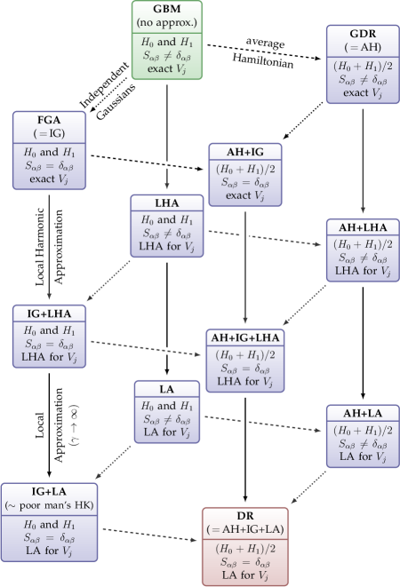
Figure 1: Approximations involved in the derivation of Dephasing Representation (DR) from the Gaussian Basis Method (GBM). The commutative diagram shows several ways to go from the–in principle exact–GBM (top) to the–usually least accurate but most efficient–DR (bottom). Different approximations are distinguished by different directions and different line types: dotted lines = Independent Gaussians (IG), dashed lines = average Hamiltonian (AH), and solid lines = Local Harmonic Approximation (LHA) or Local Approximation (LA) for the potential energy matrix elements. The figure indicates that the renormalized IG+LA value agrees in absolute value with poor man’s Herman-Kluk approximation.Tatchen et al. (2011)

III Numerical examples

In this section, the methods from Sec. II are used to compute time correlation functions required for TRSE spectra. While the efficiency of the original DR is pronounced especially in high-dimensional systems (due to its $D$-independent convergence rate mentioned in the Introduction), here we focus on few-dimensional systems which permit benchmark exact quantum calculations using the Thawed Gaussian ApproximationHeller (1975); Lee and Heller (1982) (TGA) or split-operator methods. As pointed out above, the GDR and GBM constitute a conceptual bridge between computational efficiency and formal accuracy; while both GDR and GBM converge to the exact quantum result, the number of trajectories required for convergence will certainly increase with $D$, yet—as will be clear from the examples below—this growth is typically much slower than the exponential scaling with $D$ for fixed-grid methods.

III.1 Test systems

Harmonic potential. In this model, the potential energy surface $j$ is represented by a one-dimensional harmonic potential

$$V_{j}(q)=E_{j}+\frac{1}{2}k_{j}(q-d_{j})^{2},$$ (38)

where $d_{j}$ is the displacement and $k_{j}$ the force constant. (For convenience, we set $E_{0}=E_{1}=0$, since nonzero $E_{j}$ values only shift the spectrum, but do not change its shape.)

Pyrazine $S_{0}/S_{1}$ model. This system is a simplified version of the four-dimensional vibronic coupling model, which takes into account normal modes $\nu_{1}$, $\nu_{6a}$, $\nu_{9a}$, and $\nu_{10a}$ of pyrazine.Stock et al. (1995) The $S_{0}$ and $S_{1}$ surfaces from Ref. Stock et al., 1995 are used, but the nonadiabatic coupling between states $S_{1}$ and $S_{2}$ is neglected since this coupling is much less important for the $S_{0}\rightarrow S_{1}$ excitation than for the often studied $S_{0}\rightarrow S_{2}$ excitation. This approximation was justified by two independent exact quantum calculations, with and without the $S_{1}/S_{2}$ coupling, which yielded only marginally different spectra (not shown). However, even this simplified model requires a nontrivial Duschinsky rotationDuschinsky (1937) to transform between normal modes of the ground and excited states.

Quartic oscillator. This two-dimensional system, chosen because of its chaotic dynamics,Meyer (1986); *Waterland_88; *Pollak_89; *Bohigas_93; *Revuelta_12 consists of two potential energy surfaces

$$V_{j}(q_{1},q_{2})=E_{j}+\frac{1}{2}q_{1}^{2}q_{2}^{2}+\frac{1}{4}\beta_{j}(q_{1}^{4}+q_{2}^{4}).$$ (39)

Chaotic behavior is due to the coupling term $q_{1}^{2}q_{2}^{2}/2$ since for $\beta_{j}\rightarrow\infty$ the Hamiltonian $T+$ $V_{j}$ becomes separable and hence integrable.

III.2 Computational details

The initial state was a Gaussian representing the ground vibrational state of the ground PES $V_{0}$ [in the harmonic potential (38)] or $S_{0}$ (in the pyrazine $S_{0}/S_{1}$ model). Initial states used in the quartic oscillator are specified in the figure captions. The Gaussian basis was generated with the Monte Carlo technique (with $\xi=2$ and $\epsilon=0.8$, see Appendix B.4) except in one-dimensional applications, where an equidistant phase-space grid was used (with $N_{q}=$ $N_{p}=N^{1/2}$, see Appendix B.4). The width matrix $\gamma$ from Eq. (17) was always equal to the width matrix $\Gamma$ of the initial state.

In the quartic oscillator, exact quantum-mechanical (QM) benchmark results were obtained with a fourth-order split-operator method,Wehrle, Šulc, and Vaníček (2011) whereas in the harmonic and pyrazine $S_{0}/S_{1}$ models, QM results were obtained with Heller’s TGA (Refs. Heller, 1975; Lee and Heller, 1982), which is exact in quadratic potentials. Classical trajectories were evolved with a fourth-order symplectic integrator,Wehrle, Šulc, and Vaníček (2011) while the propagation (55) of the $\mathbf{c}$ vector was performed with the exponential method (59). This was feasible because of the limited size of the basis. The propagation time steps used for the harmonic oscillator, pyrazine, and quartic oscillator were $1$ a.u., $0.2$ a.u., and $10^{-3}$, respectively. Unit mass was used unless stated otherwise.

For Gaussian initial states in quadratic potentials, the DR results were computed efficiently with the recently publishedŠulc and Vaníček (2012) Cellular Dephasing Representation (CDR). This was possible since under these conditions CDR based on a single trajectory is equivalent to the fully converged DR, which would otherwise require thousands of trajectories.Zambrano, Šulc, and Vaníček

III.3 Time-resolved stimulated emission: time correlation functions and spectra

Now we turn to the main results comparing the approximations discussed in Subsec. II.3. Three overall conclusions can be drawn from these results: First, the GBM corrects the inaccuracies of the DR. Second, in chaotic systems, a finite basis evolving with the average Hamiltonian can, surprisingly, provide more accurate results than two bases evolved separately. Third, despite its simplicity, even the original DR is useful for computing TRSE spectra. The results are presented in four groups according to whether the DR works and whether the GBM (27) converges faster than the GDR (34).

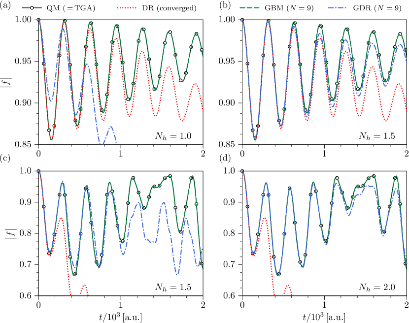
Figure 2: Time correlation function for time-resolved stimulated emission between two harmonic surfaces (38). Delay time $\tau=5000\,\text{a.u.}\approx 121\,\text{fs}$, mass $m=1250\,$a.u., and the initial state is the ground state of the ground surface $V_{0}$. $N_{h}$ gives the number of basis functions per phase-space area $h=2\pi\hbar$. Parameters in Eq. (38) are (all in a.u.): $E_{0}=E_{1}=d_{0}=0$, $d_{1}=0.08$, $k_{0}=0.5$, and (a/b) $k_{1}=0.52$: displacement is the dominant change; (c/d) $k_{1}=0.7$: change of the force constant is dominant.

GBM outperforms GDR and DR works. This occurs, e.g., in the harmonic model (38) with a large displacement $\left|d_{1}-d_{0}\right|$ and only a small change in the force constant $\left|k_{1}-k_{0}\right|$ [see Fig. 2(a)-(b)]. The figure shows that both GBM and GDR converge to the exact QM result. As expected in this simple system, GBM converges faster than GDR, in which the basis evolves with the average Hamiltonian. Convergence of GDR is accelerated by moving the $N$ Gaussians closer to one another [compare panels (a) and (b)]. While our grid is regular, a similar effect was observed in “compressed” Monte Carlo sampling.Shalashilin and Child (2008) Even the DR is rather accurate and would be exactMukamel (1982) for $k_{1}=k_{0}$.

GBM outperforms GDR and DR breaks down. The DR breaks down in simple systems such as the harmonic surfaces (38) when the force constants differ significantly. Figure 2(c) shows that the DR captures the initial decay of $f$ but not its revivals. Methods employing Gaussian bases fix this failure. GBM converges faster than GDR, although the performance of GDR is, again, improved if the basis functions are closer to one another [compare panels (c) and (d)]. Another way to partially correct the breakdown of DR is to multiply the contributions to the DR by trajectory-dependent prefactors.Zambrano and Ozorio de Almeida (2011); Zambrano, Šulc, and Vaníček Fortunately, in real systems with dissipation the recurrences in $f$ are damped, which improves the credibility of the DR.

As shown in Fig. 3(a), in the pyrazine $S_{0}/S_{1}$ model the GBM again converges to the exact QM result faster (with $N=32$) than the GDR. Although the DR does not yield correct amplitudes of the peaks, their positions are reproduced remarkably well. This is further confirmed in the TRSE spectrum in Fig. 3(b), which was computed by Fourier transforming $f$ multiplied by a phenomenological damping functionMeyer, Gatti, and Worth (2009); *Meyer:1990

$$\chi(t)=\exp(-t^{2}/T^{2}).$$ (40)

As the positions of peaks are well reproduced, one could consider this a success rather than a failure of DR. Note that the negative values present even in the exact QM spectrum in Fig. 3(b) are not numerical artifacts—unlike a continuous-wave spectrum, the TRSE spectrum defined by Eq. (6) is not guaranteed to be positive for all frequencies, although its integral over all frequencies is positive. The appearance of negative values is due to the nonstationary character of the initial state prepared by the pump pulse on the excited surface, and is discussed in detail in Ref. Pollard, Lee, and Mathies, 1990.

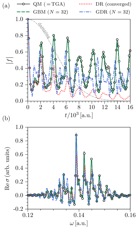
Figure 3: Time-resolved stimulated emission in the pyrazine $S_{0}/S_{1}$ model from Subsec. III.1. Initial state is the ground state of the $S_{0}$ surface and the delay time $\tau=2\cdot 10^{3}\,\text{a.u.}\approx 48\,\text{fs}$. (a) Time correlation function. The damping function of Eq. (40) with $T=6\cdot 10^{3}\,\text{a.u.}\approx 145\,\text{fs}$ is shown by a gray dash-double-dotted line. (b) Corresponding spectrum.

GDR outperforms GBM and DR works. Unexpectedly, in the chaotic quartic oscillator (39) the seemingly more approximate GDR converges faster than the GBM [see Fig. 4(a)]. Although the rapid divergence of classical trajectories aggravates the incompleteness of the Gaussian basis, this problem is much less severe in GDR. In GBM, the two bases diverge rapidly even for a small change $\left|\beta_{1}-\beta_{0}\right|$ in Eq. (39). Unless both bases cover essentially the entire available phase space, $f_{\text{GBM}}$ will decay artificially fast due to the decay of overlaps between the two bases. In contrast, GDR avoids this decay by using a single basis for dynamics on both surfaces. Unlike the GBM, which would only converge when the two bases approached completeness, the GDR converges with a very small basis since the main contribution to the decay of $f(t)$ in the chaotic quartic oscillator comes from the decay of the scalar product $\mathbf{c}_{1}(t,\,\tau)^{\dagger}\,\mathbf{c}_{0}(t,\,\tau)$ and hence is relatively insensitive to the off-diagonal elements of the overlap matrix $\mathbf{S}$. Similarly, the success of the original DR in chaotic systems relies on the use of a single Hamiltonian for propagating classical trajectories.Vaníček (2004, 2006) This explanation is confirmed in Fig. 4(a), in which GBM exhibits a spurious decay, whereas GDR (with $N=64$) agrees with the quantum result. Remarkably, due to chaotic motion, increasing $N$ up to $256$ improves the GBM result only marginally (not shown). Thanks to using the average Hamiltonian, DR matches the quantum dependence as well as the GDR, albeit at the cost of more trajectories. Comparing GDR with and without the LHA for the potential, Fig. 4(b) demonstrates that the widely used LHA breaks down completely in the quartic oscillator. In this system, matrix elements of $V$ must be treated exactly.

Figure 4: Time correlation function for time-resolved stimulated emission in quartic oscillator (39). Parameters of the potential energy surfaces are $E_{0}=E_{1}=0$ and, in the notation of Eq. (41), $\beta_{0}=0.2$ and $\delta=1/16$. Time delay $\tau=0$. Initial state is a Gaussian (17) with $\gamma_{1}=\gamma_{2}=1$ centered at $(Q_{\text{init}},\,P_{\text{init}})$, where $Q_{\text{init}}=(0,4)$ and $P_{\text{init}}=(4,0)$. (a) Comparison of various methods and their convergence as a function of $N$: GDR converges faster than GBM. ($V$ is treated exactly in both methods.) (b) Effect of the Local Harmonic Approximation (LHA) on GBM and GDR: The LHA for $V$ breaks down. ($N=64$ in all methods. In the notation of Fig. 1, GBM+LHA stands for LHA and GDR+LHA for AH+LHA. )

GDR outperforms GBM and DR breaks down. The success of the DR in chaotic systems is not universal. Figure 5 shows the time correlation function for several choices of the parameter $\beta_{0}$, controlling chaoticity, and of the difference $\Delta\beta:=\beta_{1}-\beta_{0}$ between the two surfaces. In Fig. 5, the perturbation strength is measured by parameter $\delta$, defined as

$$\delta:=\Delta\beta/\beta_{0}=\beta_{1}/\beta_{0}-1.$$ (41)

In eight of the nine Fig. 5 panels, GDR converges faster than GBM. In accordance with the heuristic arguments presented above, superiority of GDR over GBM increases with increasing chaoticity, i.e., decreasing $\beta_{0}$. This superiority disappears gradually with increasing perturbation $\delta$ due to the increasing error inherent in the propagation of the finite basis with the AH.

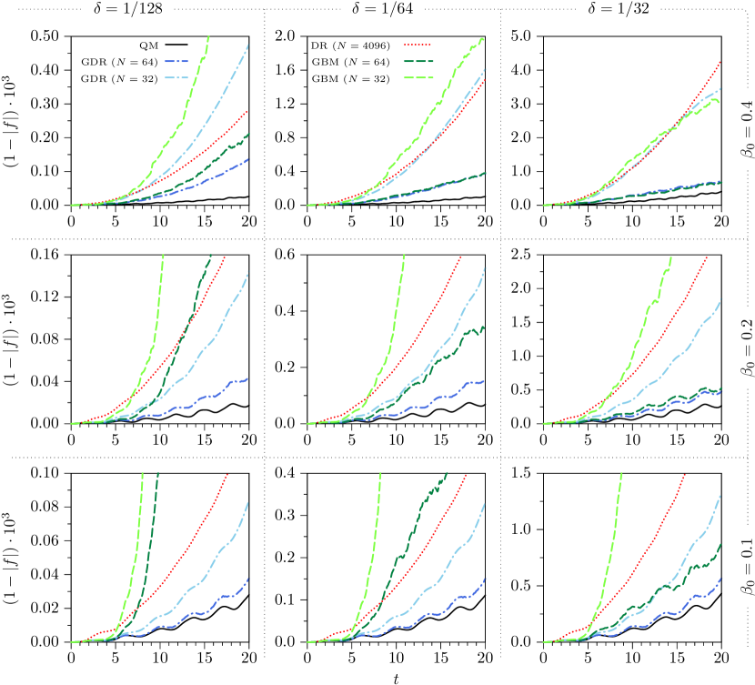
Figure 5: Time correlation function for time-resolved stimulated emission in quartic oscillator (39). Time delay $\tau=0$. Initial state is a Gaussian (17) with $\gamma_{1}=\gamma_{2}=1$ centered at the phase-space origin. Parameter $\delta$ is the relative perturbation strength defined by Eq. (41), whereas $\beta_{0}$ controls chaoticity (which increases with decreasing $\beta_{0}$). GBM and GDR results are averages over 10 realizations.

IV Conclusions

We have shown how the DR (9), an efficient semiclassical method for computing ultrafast electronic spectra, emerges naturally from the formulation of quantum dynamics in a classically evolving Gaussian basis. This was achieved by a series of three elementary approximations: evolving the basis with the AH, using IG, and applying LA for the potential. Along with the derivation based on linearizing the path integral,Shi and Geva (2005) this result puts the DR on strong theoretical footing and justifies its place among efficient semiclassical methods for computing specific time correlation functions. Moreover, the accuracy of the DR has been increased by presenting two in-principle exact generalizations of the DR: the GBM and GDR. The GBM is a straightforward application of the concept of a Gaussian basis to time correlation functions of time-resolved spectroscopy. The GDR, in contrast, is a natural generalization of the DR since (i) GDR utilizes a single basis for propagating the quantum state with both Hamiltonians, (ii) this basis propagates classically with the average Hamiltonian, and (iii) the decay of the time correlation function is due to interference and not due to decay of basis overlaps.

As expected, in many situations the GBM converges faster than the GDR. Surprisingly, in chaotic systems the GDR can outperform the GBM in which the two bases evolve separately with the “correct” Hamiltonians. Numerical results presented in Sec. III confirm that both methods achieve our main goal of increasing the accuracy of the DR in calculations of ultrafast electronic spectra. As a by-product, ten intermediate methods between the GBM and DR have been obtained, which may be useful for future applications. Relationships between all twelve methods are shown in Fig. 1, which also represents the ubiquitous balancing between formal exactness (achieved typically at a high computational cost) on one hand and computational efficiency on the other. In summary, we believe that our results provide additional insight into the connections between various exact and semiclassical methods, and demonstrate the practical value of semiclassical and Gaussian basis approaches based on classical trajectories.

Appendix A Gaussian integrals

Here we derive formulae for the $\mathbf{S}$, $\mathbf{D}$, and $\mathbf{H}$ matrix elements required in Eq. (20). All of these matrix elements can be expressed in terms of three basic integrals

$$I_{0}(A,b) :=\int\!d^{D}\!{q}\,\,e^{-{q}^{\mathrm{T}}\!\cdot{A}\cdot{q}+{b}^{\mathrm{T}}\!\cdot{q}},$$

$$I_{1}(A,b,\delta) :=\int\!d^{D}\!{q}\,\,({\delta}^{\mathrm{T}}\!\cdot{q})\,e^{-{q}^{\mathrm{T}}\!\cdot{A}\cdot{q}+{b}^{\mathrm{T}}\!\cdot{q}},$$

$$I_{2}(A,b,\kappa) :=\int\!d^{D}\!{q}\,\,({q}^{\mathrm{T}}\!\cdot{\kappa}\cdot{q})\,e^{-{q}^{\mathrm{T}}\!\cdot{A}\cdot{q}+{b}^{\mathrm{T}}\!\cdot{q}},$$

where $A$ and $\kappa$ denote $D\!\times\!D$ positive definite symmetric complex matrices, while $b$, $c$, and $\delta$ are $D$-dimensional complex vectors. The integral $I_{0}(A,b)$ is well known:Gradshteyn and Ryzhik (2007)

$$I_{0}(A,b)=\left(\frac{\pi^{D}}{\det A}\right)^{\frac{1}{2}}\exp\left(\frac{1}{4}\,b^{\mathrm{T}}\!\cdot{A^{-1}}\cdot{b}\right).$$ (42)

Since $I_{1}(A,b,\delta)=\sum_{l=1}^{D}\delta_{l}\frac{\partial}{\partial{}{b_{l}}}I_{0}(A,b)$, differentiation of Eq. (42) with respect to the components of $b$ gives

$$I_{1}(A,b,\delta)=\frac{1}{2}I_{0}(A,b)\left({\delta}^{\mathrm{T}}\!\cdot{A^{-1}}\cdot{b}\right).$$ (43)

Similarly one obtains

$$I_{2}(A,b,\kappa)=\frac{1}{4}I_{0}(A,b)\left[c^{\mathrm{T}}\!\cdot{\kappa}\cdot{c}+2\,\mathrm{Tr}\left(\kappa\,\cdot A^{-1}\right)\right],$$ (44)

where $c:={A^{-1}}\cdot{b}$, by noting that

$$I_{2}(A,b,\kappa)=\sum_{l,k=1}^{D}\frac{\partial}{\partial{}{b_{l}}}\kappa_{lk}\frac{\partial}{\partial{}{b_{k}}}I_{0}(A,b).$$

As mentioned in Sec. II, the Gaussian basis functions labeled by index $\alpha$ have the form

$$\phi_{\alpha}(q) =N_{\alpha}\exp\left[-(q-q_{\alpha})^{\mathrm{T}}\!\cdot{\gamma}\cdot(q-q_{\alpha})/2\right.$$

$$+\left.i{p_{\alpha}}^{\mathrm{T}}\!\cdot(q-q_{\alpha})/\hbar\right],$$ (45)

where the superscript $t$ denoting time dependence is omitted for simplicity. The $D\!\times\!D$ constant real matrix $\gamma$ is assumed to be independent of $\alpha$ and to be symmetric positive definite in order that the basis functions (45) be square normalizable.

Calculation of the overlap matrix $S_{\alpha\beta}=\langle\phi_{\alpha}(t)|\phi_{\beta}(t)\rangle$ is simplified by introducing vectors

$$\Delta{}q :=q_{\alpha}-q_{\beta}, Q :=(q_{\alpha}+q_{\beta})/2,$$

$$\Delta{}p :=p_{\alpha}-p_{\beta}, P :=(p_{\alpha}+p_{\beta})/2.$$

Special case of the integral $I_{0}$ [Eq. (42)] yields

$$S_{\alpha\beta} =\exp\left[-\left(\Delta{}q^{\mathrm{T}}\!\cdot{\gamma}\cdot{\Delta{}q}+\Delta{}p^{\mathrm{T}}\!\cdot{\gamma^{-1}}\cdot\Delta{}p/\hbar^{2}\right)/4\right]$$

$$\times\exp\left(i\,{\Delta{}q}^{\mathrm{T}}\!\cdot{P/}\hbar\right).$$ (46)

Application of the identity

$$D_{\alpha\beta}=\left({\dot{q}_{\beta}}^{\mathrm{T}}\!\cdot{\nabla_{\!q_{\beta}}}+{\dot{p}_{\beta}}^{\mathrm{T}}\!\cdot{\nabla_{\!p_{\beta}}}\right)S_{\alpha\beta}$$

for the time-derivative matrix elements (23) to Eq. (46) for $S_{\alpha\beta}$ gives

$$D_{\alpha\beta} =S_{\alpha\beta}\left[{\dot{p}_{\beta}}^{\mathrm{T}}\!\cdot{\left(\gamma^{-1}\cdot\Delta{}p+i\hbar\,{\Delta{}q}\right)/(2\hbar^{2})}\right.$$

$$\left.+\,{\dot{q}_{\beta}}^{\mathrm{T}}\!\cdot{\left(\gamma\cdot{\Delta{}q/2}-iP/\hbar\right)}\right].$$ (47)

As for the kinetic operator $\hat{T}$, we assume a slightly generalized form

$$\hat{T}=-\frac{\hbar^{2}}{2}\sum_{k,l=1}^{D}g_{kl}\frac{\partial^{2}}{\partial{}q_{k}\partial{}q_{l}},$$ (48)

where $g_{kl}$ represents matrix elements of a symmetric positive definite matrix $g$. (Nevertheless, all numerical calculations employed a diagonal $\hat{T}$ corresponding to $g_{kl}=\delta_{kl}m_{k}^{-1}$, i.e., $g$ was the inverse of the diagonal mass matrix $m$.) Matrix elements of $\hat{T}$ are given by

$$T_{\alpha\beta}=S_{\alpha\beta}\left[\frac{1}{2}{P^{\text{eff}}}^{\mathrm{T}}\!\cdot{g}\cdot{P^{\text{eff}}}+\frac{1}{4}\hbar^{2}\mathrm{Tr}\left(g\,\cdot\gamma\right)\right]$$ (49)

with $P^{\text{eff}}:=P+i\hbar\,{\gamma}\cdot{\Delta{}q}/2$.

It is impossible to write the potential energy matrix elements $V_{\alpha\beta}$ in a closed form for a general potential $V(q)$. One can, however, obtain a useful approximation by expanding the potential in a truncated Taylor series about the coordinate $Q$, at which the expression $\lvert\phi_{\alpha}(q)^{\star}\phi_{\beta}(q)\rvert$ attains its maximum, and by evaluating the resulting integral analytically. Adopting the multi-index notation, the potential is approximated up to the $l$th order as

$$V(q)\approx\sum_{|\lambda|=0}^{l}\left.\frac{D^{\lambda}V}{\lambda!}\right|_{Q}\cdot(q-Q)^{\lambda}.$$ (50)

Contributions to $V_{\alpha\beta}$ from individual terms in Eq. (50) are obtained by a repeated application of the differential operator $i\hbar\left(\nabla_{p_{\alpha}}-\nabla_{p_{\beta}}\right)/2$ to the overlap matrix $S_{\alpha\beta}$. As a result, one obtains the first moment

$$I_{\alpha\beta} :=\langle\phi_{\alpha}\lvert\hat{q}-Q\rvert\phi_{\beta}\rangle$$

$$=\frac{i\hbar}{2}\left(\nabla_{p_{\alpha}}-\nabla_{p_{\beta}}\right)S_{\alpha\beta}=S_{\alpha\beta}\,\rho,$$ (51)

the second moment

$$J_{\alpha\beta,rs} :=\langle\phi_{\alpha}\lvert(\hat{q}-Q)_{r}(\hat{q}-Q)_{s}\rvert\phi_{\beta}\rangle$$

$$=-\frac{\hbar^{2}}{4}\left(\nabla_{p_{\alpha}}-\nabla_{p_{\beta}}\right)_{rs}^{2}S_{\alpha\beta}$$

$$=S_{\alpha\beta}\left[\rho_{r}\rho_{s}+(1/2)\left(\gamma^{-1}\right)_{rs}\right],$$ (52)

and the third moment

$$K_{\alpha\beta,rst} :=\langle\phi_{\alpha}\lvert(\hat{q}-Q)_{r}(\hat{q}-Q)_{s}(\hat{q}-Q)_{t}\rvert\phi_{\beta}\rangle$$

$$=-\frac{i\hbar^{3}}{8}\left(\nabla_{p_{\alpha}}-\nabla_{p_{\beta}}\right)_{rst}^{3}S_{\alpha\beta}$$

$$=S_{\alpha\beta}\{\rho_{r}\rho_{s}\rho_{t}+(1/2)[(\gamma^{-1})_{rs}\rho_{t}$$

$$\ \ +(\gamma^{-1})_{st}\rho_{r}+(\gamma^{-1})_{tr}\rho_{s}]\},$$ (53)

where $\rho:=-i\gamma^{-1}\cdot{\Delta{}p/(}2\hbar)$. The fourth moment is a bit complicated to reproduce here. Nevertheless, it is easily evaluated by using Eq. (51) together with

$$\frac{i\hbar}{2}\left(\nabla_{p_{\alpha}}-\nabla_{p_{\beta}}\right)\rho=\frac{1}{2}\gamma^{-1}.$$

Appendix B Efficient numerical implementation

B.1 Numerical algorithm for the propagation equation (20)

1:

2:

• initial state $\lvert\Psi_{\text{init}}\rangle$ at time $t_{0}$, $\lvert\psi(t_{0})\rangle=\lvert\Psi_{\text{init}}\rangle$

• final propagation time $T$, time step $\Delta{}t$

• number of basis elements $N$

3:state $\lvert\psi(T)\rangle$ at time $T$

4:$t:=t_{0}$

5:expand $\lvert\Psi_{\text{init}}\rangle$ into the basis $\{\lvert\phi_{\alpha}(t)\rangle\}_{\alpha=1}^{N}$ Eqs. (15)-(16)

6:while $t\leq{}T$ do

7:    construct the $\mathbf{S}$,$\mathbf{D}$,$\mathbf{H}$ matrices Eq. (20)

8:    update the expansion coefficients $c_{\alpha}(t)$

9:    propagate classically all $N$ Gaussians by $\Delta{}t$

10:    renormalize $\lvert\psi(t)\rangle$ for norm-nonconserving propagators

11:    $t:=t+\Delta{}t$

12:end while

B.2 Factoring out the semiclassical phase factor in Eq. (20)

Propagation (20) can be accelerated by evaluating the dominant oscillatory behavior of $c_{\alpha}(t)$ semiclassically, which is achieved by factoring out the semiclassical phase factor in expansion (16):

$$|\psi(t)\rangle=\sum_{\alpha=1}^{N}\tilde{c}_{\alpha}(t)\,e^{iS_{\alpha}^{\text{cl}}(t)/\hbar}\lvert\phi_{\alpha}(t)\rangle,$$ (54)

where $S_{\alpha}^{\text{cl}}(t)=\int_{0}^{t}d\tilde{t}\,[\dot{q}_{\alpha}^{\tilde{t}}\cdot p_{\alpha}^{\tilde{t}}-H(q_{\alpha}^{\tilde{t}},p_{\alpha}^{\tilde{t}})]$ is the classical action. New coefficients $\tilde{c}_{\alpha}(t)$ are propagated according to the equation

$${\tilde{\mathbf{S}}(t)}\,{\dot{\tilde{\mathbf{c}}}(t)}=-{\left\{\frac{i}{\hbar}\left[\tilde{\mathbf{H}}(t)+\bar{\mathbf{S}}(t)\right]+\tilde{\mathbf{D}}(t)\right\}}\,{\tilde{\mathbf{c}}(t)}.$$ (55)

The modified matrices can be expressed as

$${\tilde{Z}}_{\alpha\beta}(t) =Z_{\alpha\beta}(t)\,\exp\left\{\frac{i}{\hbar}\left[S_{\beta}^{\text{cl}}(t)-S_{\alpha}^{\text{cl}}(t)\right]\right\}\text{, }$$ (56)

$${\bar{S}}_{\alpha\beta}(t) =\tilde{S}_{\alpha\beta}(t)\dot{S}_{\beta}^{\text{cl}}(t),$$ (57)

where $Z$ stands for $S$, $D$, or $H$. A similar factorization was employed by Martínez and co-workers in the Multiple SpawningBen-Nun and Martínez (2002) and by Shalashilin and co-workers in the Coupled Coherent States.Shalashilin and Child (2000); *Shalashilin_JCP_01a; *Shalashilin_JCP_01b; *Shalashilin_ChemPhys_04

B.3 Solving the propagation Eqs. (20) or (55)

Classical propagation of the basis (i.e., of $q_{\alpha}$ and $p_{\alpha}$) and the action $S_{\alpha}^{\text{cl}}$ is performed with a symplectic algorithm.Brewer, Hulme, and Manolopoulos (1997); Šulc and Vaníček (2012)  Quantum propagation (20) of the basis coefficients $c_{\alpha}$ is a more involved process: While quite sophisticated algorithmsKoonin (1998); Press et al. (2007); Levine et al. (2008) exist for similar problems, here we employed two simple methods based on dividing the propagation range $[0,\,T]$ into equal intervals of size $\Delta{}t$.

Both the implicit Euler method,

$$\mathbf{c}_{n+1}=\left[\mathbf{S}_{n+1}+\left(\frac{i}{\hbar}\mathbf{H}_{n+1}+\mathbf{D}_{n+1}\right)\Delta{}t\right]^{-1}\!\!\mathbf{S}_{n+1}\mathbf{c}_{n},$$ (58)

and the “exact” exponential method,

$$\mathbf{c}_{n+1}=\exp\left[-\mathbf{S}_{n}^{-1}\left(\frac{i}{\hbar}\mathbf{H}_{n}+\mathbf{D}_{n}\right)\Delta{}t\right]\mathbf{c}_{n},$$ (59)

are clear in the matrix notation, with subscript $n$ denoting the $n$th propagation step. In addition, the wave function was renormalized by rescaling $\mathbf{c}_{n}$ by $\left(\mathbf{c}_{n}^{\dagger}\mathbf{S}_{n}\mathbf{c}_{n}\right)^{-1/2}$ after each step. While it was essential only for the implicit Euler method, the renormalization was always performed since for sufficiently large $N$, the $\mathcal{O}(N^{2}$) cost of renormalization is negligible compared to the overall $\mathcal{O}(N^{3}$) cost of both methods. In the algorithm of Subsec. B.1, steps 4, 5, and 6 must be reordered as 6, 4, 5 for the implicit Euler method (58) since the basis must first be propagated in order to evaluate matrices at the $(n+1)$th step.

In practice, it is neither necessary nor desirable to compute the inverse matrix $\mathbf{S}_{n}^{-1}$. For example, rather than computing $\mathbf{X:=S}_{n}^{-1}\left(\frac{i}{\hbar}\mathbf{H}_{n}+\mathbf{D}_{n}\right)$ as indicated, it is preferable to solve a system of linear equations $\mathbf{S}_{n}\mathbf{X}=\frac{i}{\hbar}\mathbf{H}_{n}+\mathbf{D}_{n}$ for $\mathbf{X}$ using any standard method. In this context, Martínez and co-workers suggestedMartínez, Ben-Nun, and Ashkenazi (1996); Martínez, Ben-Nun, and Levine (1996) to use singular value decomposition;Press et al. (2007) theoretical justification was givenKay (1989) by Kay. A different approach, consisting in inverting $\mathbf{S}_{n}$ by an iterative algebraic procedure was exploredAndersson (2001) by Andersson.

Due to matrix exponentiation, the exponential method (59) is feasible only for smaller basis sets. Although presumably exact, this method does not necessarily permit a larger time step $\Delta t$ than the first-order implicit Euler method with renormalization. The reason is that for badly conditioned $\mathbf{S}_{n}$, eigenvalues of the matrix $\mathbf{S}_{n}^{-1}\left(\frac{i}{\hbar}\mathbf{H}_{n}+\mathbf{D}_{n}\right)\Delta{}t$ become large except for very small time step $\Delta t$. Since most numerical methods for matrix exponentiation require eigenvalues of the exponentiated matrix to be small,Sidje (1998) lowering $\Delta t$ is required.

Sawada et al. proposedSawada et al. (1985) to monitor eigenvalues of $\mathbf{S}_{n}$ during propagation, concluding that the basis size was insufficient if all eigenvalues were (in absolute value) close to $1$. In contrast, if some eigenvalues are very small, some functions should be removed in order to restore regularity of $\mathbf{S}_{n}$. Such features, however, have not been implemented here.

In our calculations, the exponential method allows a much larger time step than the implicit Euler method (both in the pyrazine $S_{0}/S_{1}$ model and in the quartic oscillator, see Fig. 6). Figure 6 also suggests that the modified propagation Eq. (55) from Appendix B.2 permits increasing the time step in comparison with the original propagation Eq. (20). This improvement is more pronounced in the implicit Euler method (58) than in the exponential method (59).

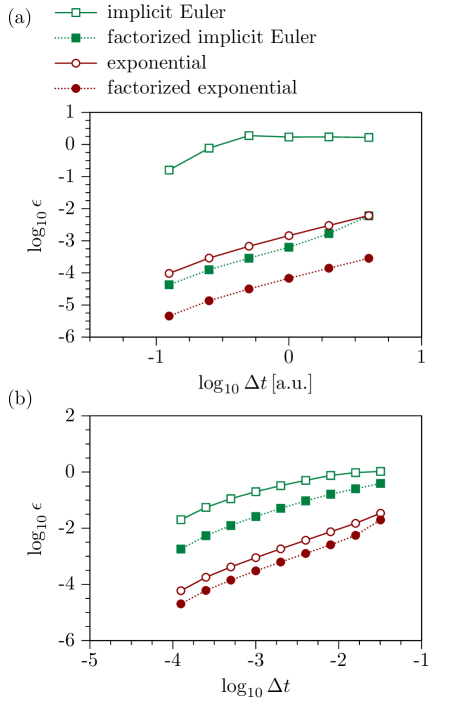
Figure 6: Error of the correlation function $f$ computed with the GBM as a function of time step $\Delta t$. The figure compares the normalized $L^{2}$ errors $\epsilon_{\Delta t}:=\left\|f_{\Delta t}-f\right\|/\left\|f\right\|$ on the time interval $[0,T]$ obtained with the implicit Euler method (58) and exponential method (59) applied to the propagation Eqs. (20) or (55) [without and with the semiclassical factorization (54)]. (a) Pyrazine $S_{0}/S_{1}$ model ($N=32$, $T=18000$ a.u., other parameters as in Fig. 3). (b) Quartic oscillator ($N=32$, $T=12$, other parameters as in Fig. 4).

B.4 Choice of the basis in Eq. (16)

Another numerical issue is the choice of basis in Eq. (16), which must represent $\lvert\Psi_{\text{init}}\rangle$ properly. A small approximation error (in the $L^{2}$ sense) in Eq. (16), however, does not guarantee quality of the basis at later times. In general, a compromise is required between the size of the basis and its acceptability from the dynamical point of view.

Two methods used for the Sec. III calculations are described below, with more thorough discussions available elsewhere.Burant and Batista (2002); Davis and Heller (1979); Shalashilin and Child (2008) To keep notation simple, we assume that $D=1$ and consider the initial state to be a Gaussian (17):

$$\lvert\Psi_{\text{init}}\rangle:=\lvert\Gamma,Q,P\rangle.$$ (60)

Equidistant phase-space basis functions are constructed as

$$\phi_{\alpha}(q)=\langle{q}|\gamma,q_{i},p_{j}\rangle,\quad\alpha=iN_{p}+j,$$

where

$$\begin{split}q_{i}&=Q+\frac{2i-(N_{q}-1)}{2}\Delta{}q,\quad 0\leq{}i<N_{q},\\ p_{j}&=P+\frac{2j-(N_{p}-1)}{2}\Delta{}p,\quad 0\leq{}j<N_{p}.\end{split}$$ (61)

Symbols $N_{q}$ and $N_{p}$ represent the numbers of points in the corresponding phase-space coordinates. The size of basis is $N=N_{q}N_{p}$.

Grid spacings $\Delta{}q$ and $\Delta{}p$ are chosen to ensure a given number $N_{h}$ of basis functions per phase-space area $h=2\pi\hbar$ and a constant absolute value of overlap between neighboring functions with the same index $i$ or $j$. These requirements imply

$$\Delta{}q=\sqrt{\frac{2\pi}{N_{h}\gamma}}\,\text{ and }\,\Delta{}p=\hbar\sqrt{\frac{2\pi\gamma}{N_{h}}}.$$ (62)

Since the basis is nonorthogonal, ensuring fixed overlap between neighboring functions does not guarantee constant linear independence of the basis with increasing $N$, as illustrated in Fig. 7, which shows the dependence of the condition number $\kappa$ of the overlap matrix $\mathbf{S}$ on $N$.

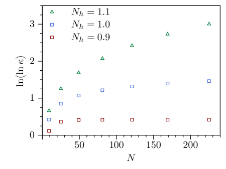
Figure 7: Dependence of the condition number $\kappa$ of the overlap matrix (21) on the size $N$ and density of the basis constructed according to Eq. (61). $D=1$, $\gamma=1$, and $N_{h}$ denotes the number of basis functions per phase-space area $h=2\pi\hbar$.

Monte Carlo basis is generated with an algorithmKay (1994); Ben-Nun, Quenneville, and Martínez (2000); Shalashilin and Child (2008) sampling the coherent-state basis functions from the absolute value of the overlap $\chi:=\langle\gamma,q,p|\Gamma,Q,P\rangle$ of the initial state (60) with a basis state $\lvert\gamma,q,p\rangle$ of Eq. (17). The absolute value of this overlap, understood as a function of $q$ and $\,p$, is

$$\lvert\chi(q,\,p)\rvert^{2}\propto\exp\left[-\frac{\gamma\Gamma}{\gamma+\Gamma}(q-Q)^{2}-\frac{1}{\hbar^{2}}\frac{(p-P)^{2}}{\gamma+\Gamma}\right].$$ (63)

The overall procedure is as follows:

1:

2:

• desired number of basis elements $N$

• parameters $\xi>0$, $\gamma>0$, and $1>\epsilon>0$

3:Gaussian basis used in Eq. (16)

4:$\alpha:=1$

5:while $\alpha\leq{}N$ do

6:    sample $q,\,p$ from the distribution $\sim$ $\lvert\chi(q,\,p)\rvert^{2\xi}$

7:    $\eta:=\text{sup}_{1\leq{}\beta<\alpha}\lvert\langle\phi_{\beta}|\gamma,q,p\rangle\rvert$

8:    if $\eta<\epsilon$ then

9:         $\lvert\phi_{\alpha}\rangle:=\lvert\gamma,q,p\rangle$

10:         $\alpha:=\alpha+1$

11:    end if

12:end while

The conditional statement in step $5$ is added to improve the condition number $\kappa$ of the resulting overlap matrix$~{}\mathbf{S}$.Ben-Nun and Martínez (2002) A modified approach based on orthogonal projections was proposedWu and Batista (2003) by Wu and Batista in their Matching-Pursuit Split-Operator Fourier-Transform technique.

References

- Bisgaard et al. (2009) C. Z. Bisgaard, O. J. Clarkin, G. Wu, A. M. D. Lee, O. Gessner, C. C. Hayden, and A. Stolow, Science 323, 1464 (2009).
- Bressler et al. (2009) C. Bressler, C. Milne, V.-T. Pham, A. ElNahhas, R. M. van der Veen, W. Gawelda, S. Johnson, P. Beaud, D. Grolimund, M. Kaiser, C. N. Borca, G. Ingold, R. Abela, and M. Chergui, Science 323, 489 (2009).
- Carbone, Kwon, and Zewail (2009) F. Carbone, O.-H. Kwon, and A. H. Zewail, Science 325, 181 (2009).
- Miller (2001) W. H. Miller, J. Phys. Chem. A 105, 2942 (2001).
- Herman (1994) M. F. Herman, Annu. Rev. Phys. Chem. 45, 83 (1994).
- Thoss and Wang (2004) M. Thoss and H. Wang, Annu. Rev. Phys. Chem. 55, 299 (2004).
- Kay (2005) K. G. Kay, Annu. Rev. Phys. Chem. 56, 255 (2005).
- Meyer, Gatti, and Worth (2009) H.-D. Meyer, F. Gatti, and G. A. Worth, eds., Multidimensional Quantum Dynamics: MCTDH Theory and Applications, 1st ed. (Wiley-VCH, Weinheim, 2009).
- Meyer, Manthe, and Cederbaum (1990) H.-D. Meyer, U. Manthe, and L. Cederbaum, Chem. Phys. Lett. 165, 73 (1990).
- Burghardt, Meyer, and Cederbaum (1999) I. Burghardt, H.-D. Meyer, and L. S. Cederbaum, J. Chem. Phys. 111, 2927 (1999).
- Ben-Nun and Martínez (2002) M. Ben-Nun and T. J. Martínez, Adv. Chem. Phys. 121, 439 (2002).
- Tatchen and Pollak (2009) J. Tatchen and E. Pollak, J. Chem. Phys. 130, 041103 (2009).
- Ceotto et al. (2009) M. Ceotto, S. Atahan, G. F. Tantardini, and A. Aspuru-Guzik, J. Chem. Phys. 130, 234113 (2009).
- Ceotto, Zhuang, and Hase (2013) M. Ceotto, Y. Zhuang, and W. L. Hase, J. Chem. Phys. 138, 054116 (2013).
- Thompson and Martínez (2011) A. L. Thompson and T. J. Martínez, Faraday Discuss. 150, 293 (2011).
- Worth, Robb, and Burghardt (2004) G. A. Worth, M. A. Robb, and I. Burghardt, Faraday Discuss. 127, 307 (2004).
- Worth, Robb, and Lasorne (2008) G. Worth, M. Robb, and B. Lasorne, Mol. Phys. 106, 2077 (2008).
- Saita and Shalashilin (2012) K. Saita and D. V. Shalashilin, J. Chem. Phys. 137, 22A506 (2012).
- Vaníček (2004) J. Vaníček, Phys. Rev. E 70, 055201 (2004).
- Vaníček (2006) J. Vaníček, Phys. Rev. E 73, 046204 (2006).
- Wehrle, Šulc, and Vaníček (2011) M. Wehrle, M. Šulc, and J. Vaníček, Chimia 65, 334 (2011).
- Šulc and Vaníček (2012) M. Šulc and J. Vaníček, Mol. Phys. 110, 945 (2012).
- Mukamel (1982) S. Mukamel, J. Chem. Phys. 77, 173 (1982).
- Mukamel (1999) S. Mukamel, Principles of nonlinear optical spectroscopy, 1st ed. (Oxford University Press, New York, 1999).
- Shi and Geva (2005) Q. Shi and E. Geva, J. Chem. Phys. 122, 064506 (2005).
- McRobbie et al. (2009) P. L. McRobbie, G. Hanna, Q. Shi, and E. Geva, Acc. Chem. Res. 42, 1299 (2009).
- Wang, Sun, and Miller (1998) H. Wang, X. Sun, and W. H. Miller, J. Chem. Phys. 108, 9726 (1998).
- note (2) Some authorsShi and Geva (2005); McRobbie et al. (2009) refer to the DR as the LSC-IVR since the DR can be understood as a linearized semiclassical approximation for fidelity amplitude.Shi and Geva (2005); Vaníček (2006) However, in the notation of Sec. II, LSC-IVR usually refers to the approximationWang, Sun, and Miller (1998) , which can be also used to approximate fidelity (i.e., fidelity amplitude squared),Vaníček (2006) but does not include any quantum dynamical effects; the only quantum effects are static, arising from replacing classical observables by their Wigner transforms. Therefore we prefer avoiding the name LSC-IVR when referring to the DR of fidelity amplitude, since the DR does incorporate dynamical interference effects even when the description based on the LSC-IVR of fidelity is purely classical.
- Li, Fang, and Martens (1996) Z. Li, J.-Y. Fang, and C. C. Martens, J. Chem. Phys. 104, 6919 (1996).
- Egorov, Rabani, and Berne (1998) S. A. Egorov, E. Rabani, and B. J. Berne, J. Chem. Phys. 108, 1407 (1998).
- Egorov, Rabani, and Berne (1999) S. A. Egorov, E. Rabani, and B. J. Berne, J. Chem. Phys. 110, 5238 (1999).
- Shemetulskis and Loring (1992) N. E. Shemetulskis and R. F. Loring, J. Chem. Phys. 97, 1217 (1992).
- Rost (1995) J. M. Rost, J. Phys. B 28, L601 (1995).
- Zimmermann and Vaníček (2012a) T. Zimmermann and J. Vaníček, J. Chem. Phys. 136, 094106 (2012a).
- Zimmermann and Vaníček (2012b) T. Zimmermann and J. Vaníček, J. Chem. Phys. 137, 22A516 (2012b).
- Petitjean et al. (2007) C. Petitjean, D. V. Bevilaqua, E. J. Heller, and P. Jacquod, Phys. Rev. Lett. 98, 164101 (2007).
- Zimmermann and Vaníček (2010) T. Zimmermann and J. Vaníček, J. Chem. Phys. 132, 241101 (2010).
- Li, Mollica, and Vaníček (2009) B. Li, C. Mollica, and J. Vaníček, J. Chem. Phys. 131, 041101 (2009).
- Zimmermann et al. (2010) T. Zimmermann, J. Ruppen, B. Li, and J. Vaníček, Int. J. Quant. Chem. 110, 2426 (2010).
- Wang et al. (2005) W. Wang, G. Casati, B. Li, and T. Prosen, Phys. Rev. E 71, 037202 (2005).
- Ares and Wisniacki (2009) N. Ares and D. A. Wisniacki, Phys. Rev. E 80, 046216 (2009).
- Wisniacki, Ares, and Vergini (2010) D. A. Wisniacki, N. Ares, and E. G. Vergini, Phys. Rev. Lett. 104, 254101 (2010).
- García-Mata and Wisniacki (2011) I. García-Mata and D. A. Wisniacki, J. Phys. A 44, 315101 (2011).
- Thompson and Makri (1999) K. Thompson and N. Makri, Phys. Rev. E 59, R4729 (1999).
- Kühn and Makri (1999) O. Kühn and N. Makri, J. Phys. Chem. A 103, 9487 (1999).
- Mollica and Vaníček (2011) C. Mollica and J. Vaníček, Phys. Rev. Lett. 107, 214101 (2011).
- Heller (1991) E. J. Heller, J. Chem. Phys. 94, 2723 (1991).
- Zambrano and Ozorio de Almeida (2011) E. Zambrano and A. M. Ozorio de Almeida, Phys. Rev. E 84, 045201(R) (2011).
- Burghardt, Giri, and Worth (2008) I. Burghardt, K. Giri, and G. A. Worth, J. Chem. Phys. 129, 174104 (2008).
- Martínez, Ben-Nun, and Ashkenazi (1996) T. J. Martínez, M. Ben-Nun, and G. Ashkenazi, J. Chem. Phys. 104, 2847 (1996).
- Martínez, Ben-Nun, and Levine (1996) T. J. Martínez, M. Ben-Nun, and R. D. Levine, J. Phys. Chem. 100, 7884 (1996).
- Sawada et al. (1985) S.-I. Sawada, R. Heather, B. Jackson, and H. Metiu, J. Chem. Phys. 83, 3009 (1985).
- Heather and Metiu (1985) R. Heather and H. Metiu, Chem. Phys. Lett. 118, 558 (1985).
- Heather and Metiu (1986) R. Heather and H. Metiu, J. Chem. Phys. 84, 3250 (1986).
- Shalashilin and Child (2000) D. V. Shalashilin and M. S. Child, J. Chem. Phys. 113, 10028 (2000).
- Shalashilin and Child (2001a) D. V. Shalashilin and M. S. Child, J. Chem. Phys. 114, 9296 (2001a).
- Shalashilin and Child (2001b) D. V. Shalashilin and M. S. Child, J. Chem. Phys. 115, 5367 (2001b).
- Shalashilin and Child (2004) D. V. Shalashilin and M. S. Child, Chem. Phys. 304, 103 (2004).
- Pollard, Lee, and Mathies (1990) W. T. Pollard, S.-Y. Lee, and R. A. Mathies, J. Chem. Phys. 92, 4012 (1990).
- Tannor (2004) D. J. Tannor, Introduction to Quantum Mechanics: A Time-Dependent Perspective (University Science Books, Sausalito, California, 2004).
- Gorin et al. (2006) T. Gorin, T. Prosen, T. H. Seligman, and M. Žnidarič, Phys. Rep. 435, 33 (2006).
- Jacquod and Petitjean (2009) P. Jacquod and C. Petitjean, Adv. Phys. 58, 67 (2009).
- Pastawski et al. (2000) H. M. Pastawski, P. R. Levstein, U. G., R. J., and H. J., Physica A 283, 166 (2000).
- Cucchietti et al. (2003) F. M. Cucchietti, D. A. R. Dalvit, J. P. Paz, and W. H. Zurek, Phys. Rev. Lett. 91, 210403 (2003).
- Vaníček and Heller (2003) J. Vaníček and E. J. Heller, Phys. Rev. E 68, 056208 (2003).
- Miller and Smith (1978) W. H. Miller and F. T. Smith, Phys. Rev. A 17, 939 (1978).
- Hubbard and Miller (1983) L. M. Hubbard and W. H. Miller, J. Chem. Phys. 78, 1801 (1983).
- Poulsen, Nyman, and Rossky (2003) J. A. Poulsen, G. Nyman, and P. J. Rossky, J. Chem. Phys. 119, 12179 (2003).
- Bonella and Coker (2005) S. Bonella and D. F. Coker, J. Chem. Phys. 122, 194102 (2005).
- Huo and Coker (2011) P. Huo and D. F. Coker, J. Chem. Phys. 135, 201101 (2011).
- Heller (1975) E. J. Heller, J. Chem. Phys. 62, 1544 (1975).
- Davis and Heller (1979) M. J. Davis and E. J. Heller, J. Chem. Phys. 71, 3383 (1979).
- Heller (1981) E. J. Heller, J. Chem. Phys. 75, 2923 (1981).
- Beck et al. (2000) M. Beck, A. Jäckle, G. Worth, and H.-D. Meyer, Phys. Rep. 324, 1 (2000).
- Heller (2006) E. J. Heller, Acc. Chem. Res. 39, 127 (2006).
- Heller (1976) E. J. Heller, J. Chem. Phys. 64, 63 (1976).
- Skodje and Truhlar (1984) R. T. Skodje and D. G. Truhlar, J. Chem. Phys. 80, 3123 (1984).
- note (1) Gaussian state is obtained in two consecutive steps: the initial frozen Gaussian is first propagated on the excited surface for time and then on the th surface for time . States and are therefore identical.
- Shalashilin (2010) D. V. Shalashilin, J. Chem. Phys. 132, 244111 (2010).
- Tatchen et al. (2011) J. Tatchen, E. Pollak, G. Tao, and W. H. Miller, J. Chem. Phys. 134, 134104 (2011).
- Lee and Heller (1982) S.-Y. Lee and E. J. Heller, J. Chem. Phys. 76, 3035 (1982).
- Stock et al. (1995) G. Stock, C. Woywod, W. Domcke, T. Swinney, and B. S. Hudson, J. Chem. Phys. 103, 6851 (1995).
- Duschinsky (1937) F. Duschinsky, Acta Physicochim. URSS 7, 551 (1937).
- Meyer (1986) H.-D. Meyer, J. Chem. Phys. 84, 3147 (1986).
- Waterland et al. (1988) R. L. Waterland, J.-M. Yuan, C. C. Martens, R. E. Gillilan, and W. P. Reinhardt, Phys. Rev. Lett. 61, 2733 (1988).
- Eckhardt, Hose, and Pollak (1989) B. Eckhardt, G. Hose, and E. Pollak, Phys. Rev. A 39, 3776 (1989).
- Bohigas, Tomsovic, and Ullmo (1993) O. Bohigas, S. Tomsovic, and D. Ullmo, Phys. Rep. 223, 43 (1993).
- Revuelta et al. (2012) F. Revuelta, E. G. Vergini, R. M. Benito, and F. Borondo, Phys. Rev. E 85, 026214 (2012).
- (89) E. Zambrano, M. Šulc, and J. Vaníček, In preparation.
- Shalashilin and Child (2008) D. V. Shalashilin and M. S. Child, J. Chem. Phys. 128, 054102 (2008).
- Gradshteyn and Ryzhik (2007) I. S. Gradshteyn and I. M. Ryzhik, Table of Integrals, Series, and Products, 7th ed. (Academic Press, San Diego, 2007).
- Brewer, Hulme, and Manolopoulos (1997) M. L. Brewer, J. S. Hulme, and D. E. Manolopoulos, J. Chem. Phys. 106, 4832 (1997).
- Koonin (1998) S. Koonin, Computational Physics: Fortran version (Westview Press, 1998).
- Press et al. (2007) W. H. Press, S. A. Teukolsky, W. T. Vetterling, and B. P. Flannery, Numerical Recipes, The art of scientific computing, 3rd ed. (Cambridge University Press, 2007).
- Levine et al. (2008) B. G. Levine, J. D. Coe, A. M. Virshup, and T. J. Martínez, Chem. Phys. 347, 3 (2008).
- Kay (1989) K. G. Kay, Chem. Phys. 137, 165 (1989).
- Andersson (2001) L. M. Andersson, J. Chem. Phys. 115, 1158 (2001).
- Sidje (1998) R. Sidje, ACM Trans. Math. Softw. 24, 130 (1998).
- Burant and Batista (2002) J. C. Burant and V. S. Batista, J. Chem. Phys. 116, 2748 (2002).
- Kay (1994) K. G. Kay, J. Chem. Phys. 100, 4432 (1994).
- Ben-Nun, Quenneville, and Martínez (2000) M. Ben-Nun, J. Quenneville, and T. J. Martínez, J. Phys. Chem. A 104, 5161 (2000).
- Wu and Batista (2003) Y. Wu and V. S. Batista, J. Chem. Phys. 118, 6720 (2003).