Empirical Links between XRB and AGN accretion using
the complete z$<$0.4 spectroscopic CSC/SDSS Catalog

Abstract

Striking similarities have been seen between accretion signatures of Galactic X-ray binary (XRB) systems and active galactic nuclei (AGN). XRB spectral states show a V-shaped correlation between X-ray spectral hardness and Eddington ratio as they vary, and some AGN samples reveal a similar trend, implying analogous processes at vastly larger masses and timescales. To further investigate the analogies, we have matched 617 sources from the Chandra Source Catalog to SDSS spectroscopy, and uniformly measured both X-ray and optical spectral characteristics across a broad range of AGN and galaxy types. We provide useful tabulations of X-ray spectral slope for broad and narrow line AGN, star-forming and passive galaxies and composite systems, also updating relationships between optical (H$\alpha$ and [O III]) line emission and X-ray luminosity. We further fit broadband spectral energy distributions with a variety of templates to estimate bolometric luminosity. Our results confirm a significant trend in AGN between X-ray spectral hardness and Eddington ratio expressed in X-ray luminosity, albeit with significant dispersion. The trend is not significant when expressed in the full bolometric or template-estimated AGN luminosity. We also confirm a relationship between the X-ray/optical spectral slope $\alpha_{\rm ox}$  and Eddington ratio, but it may not follow the trend predicted by analogy with XRB accretion states.

1. Introduction

There is now strong evidence that powerful active galactic nuclei (AGN) play a key role in the evolution of galaxies. The correlation of central black hole (M_BH) and stellar bulge mass (e.g. Gultekin et al. 2009; 2012), and the similarity between the cosmic star formation history (e.g. Hopkins $\&$ Beacom 2006) and cosmic M_BH assembly history (e.g. Aird et al 2010) both suggest that the growth of supermassive black holes (SMBH) is related to the growth of host galaxies. Understanding what drives the formation and co-evolution of galaxies and their central SMBHs remains one of the most significant challenges in extragalactic astrophysics. Understanding the feedback mechanisms, hence the AGN energy production, remains a fundamental question that needs to be answered.

Recent attention has focused on models where AGN feedback regulates the star formation in the host galaxy. These scenarios are consistent with the $M_{\rm BH}$ - $\sigma$ relation and make various predictions for AGN properties, including the environmental dependence of the AGN/galaxy interplay and the relative timing of periods of peak star formation and nuclear accretion activity. The key feature of these models is that they can potentially link the apparently independent observed relations between star formation, AGN activity and large scale structure to the same underlying physical process. For example, in the “radio-mode” model of Croton et al. (2006), accretion of gas from cooling flows in dense environments (e.g. group, cluster) may produce relatively low-luminosity AGN, which in turn heat the bulk of the cooling gas and prevent it from falling into the galaxy center to form stars. Alternatively, Hopkins et al. (2006) propose that mergers trigger luminous QSOs and circumnuclear starbursts, which both feed and obscure the central engine for most of its active lifetime. In this scenario, AGN outflows eventually sweep away the dust and gas clouds, thereby quenching the star formation. This “QSO-mode” likely dominates in poor environments (e.g. field, group), as the high-velocity encounters, common in dense regions, do not favour mergers. These proposed models make clear, testable predictions about the properties of AGN, while observational constraints provide first-order confirmation of this theoretical picture (e.g. Trichas et al. 2009; 2012). Merger-driven scenarios for example, predict an association between optical morphological disturbances, star formation and an intense obscured AGN phase in low density regions. The “radio mode” model, in contrast, invokes milder AGN activity in early-type hosts and relatively dense environments with little or no star formation.

Low-redshift galaxies offer the best observational testbeds to study quasar evolution. While environmental studies of nearby AGN are consistent with non- merger-driven fueling (Constantin $\&$ Vogeley 2006; Constantin, Hoyle, $\&$ Vogeley 2008), analysis of the observed distribution of Eddington ratios as a function of the BH masses suggest that at z$\sim$0 there might be two distinct regimes of BH growth, which are determined by the supply of cold gas in the host bulge (Kauffmann $\&$ Heckman 2009). Optical studies of narrow emission line galaxies using emission line ratio diagnostics (e.g. Trichas et al. 2010; Kalfountzou et al. 2011) although quite successful in identifying cases where the dominant mechanism is either accretion onto a black hole or radiation from hot young stars, remain inconclusive for LINERs and composite objects. However, using the latter method, Constantin et al. (2009) revealed a sequence from SF via AGN to quiescence which may be the first empirical evidence for a duty cycle analogous to that of the high-z quasars.

The X-ray emission arguably affords, the most sensitive test for measurements of the intensity and efficiency of accretion. Combining X-ray properties with optical emission line ratios for a large unbiased sample of low redshift galaxies can be especially useful because of the high quality diagnostics available. The Chandra Source Catalog (Evans et al. 2010) when cross-matched with the SDSS, provides an unprecedented number of galaxies in the local Universe for which we can combine measurements of both the X-ray and optical emission. Previous studies of the relation between the X-ray nuclear emission, optical emission line activity and black hole masses provide important physical constraints to the AGN accretion. The conclusions are that low-luminosity AGN (LLAGN) are probably scaled down versions of more luminous AGN (e.g., Panessa et al. 2006), and that $M_{\rm BH}$ is not the main driver of the X-ray properties (Greene $\&$ Ho 2007). The LLAGN are claimed to be X-ray detected at relatively high rates, and are found to be relatively unabsorbed (e.g. Miniutti et al. 2009), with the exception of those known to be Compton thick. Nonetheless, the X-ray investigations of AGN activity at its lowest levels remain largely restricted to LINERs and Seyferts.

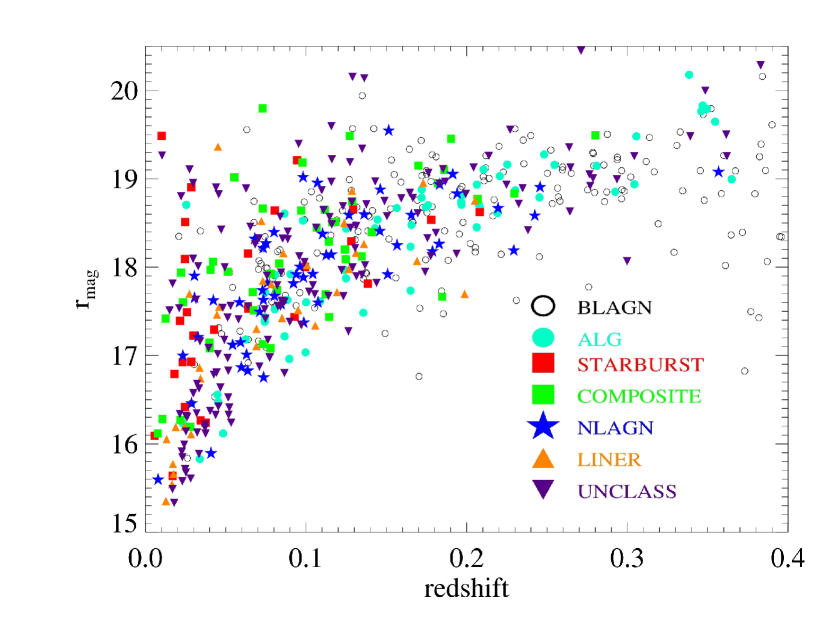
Figure 1.— Dereddened SDSS $r$ band mag (modelMag) plotted against redshift for our full $z<0.4$ spectroscopic sample detected in the Chandra Source Catalog v1.1. Black open circles are broad line AGN, cyan filled circles are absorption line galaxies (ALG), blue stars are narrow-line AGN (NLAGN), red squares are star-forming galaxies (STARBURST), orange triangles are low ionization narrow emission line region galaxies (LINERs), green squares are composite systems, and magenta downward triangles are unclassified sources.

In this work, we utilize the largest ever sample of galaxies with available optical spectroscopy and X-ray detections, a total of 617 sources, to build on the work done by Constantin et al. (2009). We combine the CSC X-ray detections with a sample of SDSS DR7 spectroscopically identified nearby galaxies that includes broad line objects, creating a large sample of galaxy nuclei that spans a range of optical spectral types, from absorption line (passive) to actively line emitting systems, including the star-forming and actively accreting types, along with those of mixed or ambiguous ionization. Our main goal is try to verify whether we see the same turning point found by both Constantin et al. (2009) and Wu $\&$ Gu (2008)in the $\Gamma$ - LŁ_Edd relation that occurs around $\Gamma$=1.5. This is identical to what stellar mass X-ray binaries exhibit, indicating that there is probably an intrinsic switch in the accretion mode, from advection-dominated flows to standard (disk/corona) accretion modes.

2. Sample Definition and Data Analysis

Our sample has been obtained by cross-matching the SDSS DR7 spectroscopic sample with the Chandra Source Catalog. We began with a Bayesian-selected 2cross-match of the Chandra Source Catalog (CSC Rev1.1; Evans et al. 2010) and the SDSS (York et al. 2000), performed by the Chandra X-ray Center (CXC; Rots et al. 2009), containing 16852 objects with both X-ray detections and optical photometric objects in SDSS DR7. Detailed visual inspection of matches was performed to eliminate obviously saturated optical sources, or uncertain counterparts in either band. Since both redshifts and emission line measurements are required for this study, the sample was further restricted to objects for which there also exist SDSS optical spectra, leaving $\sim$2000 objects.

To take advantage of the diagnostic power of the H$\alpha$/[NII] emission line complex, we set a limit of z$<$0.392 as for the Constantin et al. (2009) sample, yielding 739 objects; of these, 685 are new relative to the aforementioned sample. The SDSS spectra for all 739 objects were downloaded and checked by eye to exclude objects with serious artifacts in the spectrum or with grossly incorrect redshifts. The latter included primarily stars and several broad absorption line quasars. Upon completion, 714 spectra remained, corresponding to 682 distinct objects.

A number of the objects are present in multiple Chandra obsids. For simplicity, we merely selected the best observation to use in the X-ray spectral fitting, primarily favoring the smallest off axis angle (OAA, $\theta$) and the longest exposure time. Upon further analysis of the available X-ray data, we rejected 50 objects that were either saturated, or too close to a chip edge.

2.1. Optical Spectroscopic Analysis

We limit the investigation to z$\buildrel<\over{\sim}$0.4 so that the $H{\alpha}$ and other key emission lines are available within the wavelength range of the SDSS spectrograph to perform classic emission line ratio classification (e.g., Baldwin, Phillips & Terlevich 1981 - BPT hereafter; Kewley et al. 2006). We fit optical spectra as described in Zhou et al. (2006), beginning with starlight (using galaxy templates of Lu et al. 2006) and nuclear emission (power-law) components that also account for reddening, blended Fe II emission and Balmer continuum fitting. Iterative emission line fitting follows, using multiple Gaussian or Lorentzian profiles where warranted to fit broad and narrow line components. Best template fits of the underlying host star light provide estimates of the stellar mass, $M_{\rm BH}$ (via $\sigma_{*}$), along with mean stellar ages via the strength of the 4000Å-break and the H$\delta$ Balmer absorption line.

The optical spectral measurements include stellar velocity dispersions with errors for all galaxies as well as measurements of numerous emission line fluxes. For the broad -line objects we measure the full width at half maximum (FWHM) of the H$\beta$ emission line. Additionally, the AGN flux at 5100Å  is calculated for these objects, along with the AGN fraction of the total continuum. Unlike previous studies, this method enables us to use spectroscopic analysis that is as uniform as possible for a diverse sample.

For our broad line objects, black hole masses have been retrieved either from Shen et al (2011), who have compiled virial black hole mass estimates of all SDSS DR7 QSOs using Vestergaard $\&$ Peterson (2006) calibrations for H$\beta$ and C$\,IV$ and their own calibrations for Mg$\,II$. For other broad-line AGN (BLAGN) - predominantly those spatially-resolved Sy 1s that are not targeted by the SDSS QSO programs - we use our own H$\beta$ emission line fits. For all galaxies lacking broad emission lines, we use our measurements of $\sigma_{*}$ to calculate M_BH values using the M-$\sigma$ relation of Graham et al. (2011).

The number of objects with successful spectral analysis includes both broad and narrow emission line galaxies, totaling 617 in our final sample. Figure 1 shows the de-reddened $r$ band magnitude (SDSS modelMag) for the sample, plotted against redshift.

2.2. Multi-wavelength Data

A prime advantage of our CSC/SDSS sample, in comparison to deeper pencil-beam X-ray surveys, is its relatively shallow depth that allows for easier source identification in other wavelengths. We have cross-correlated our spectroscopic sample with publicly available GALEX (DR6; Morrissey et al. 2007), UKIDSS (DR4; Lawrence et al. 2007), 2MASS (Skrutskie et al. 2006), VLA (Becker et al. 1995) and WISE (Wright et al. 2010) catalogs. We have retrieved these catalogs using the Virtual Observatory (VO) TOPCAT tool (Taylor 2005). Using Monte-Carlo simulations and the Fadda et al (2002) method, we have concluded that a search radius of 2.5 arcsec provides us with a $P(d)$ $<$ 0.02, where $P(d)$ is the Poisson probability of a GALEX source to have a random association within a distance $d$, yielding an expected rate of random associations of less than 5$\%$. The GALEX catalog contains only sources that were detected at S/N $>$ 5 in at least one of the NUV, FUV filters. All matches were then visually inspected to remove any apparent spurious associations. We have adopted a similar method for the catalogs at other wavebands.

3. OPTICAL SPECTRAL CLASSIFICATION

To classify emission line sources we use BPT diagnostic diagrams, which employ four line flux ratios: [O III]5007/H$\beta$, [N II]6583/H$\alpha$, [S II]6716,6731/H$\alpha$ and [O I]6300/H$\alpha$. We only consider emission lines detected with at least 2$\sigma$ confidence. Following Kewley et al. (2006) classification criteria, the emission line objects are separated into Seyferts, LINERs, composite objects and star-forming galaxies. A quite large (25$\%$) fraction of the emission-line objects remains unclassified as their line ratios, although accurately measured, do not correspond to a clear spectral type in the two diagrams. For the majority, while the [N II]/H$\alpha$ ratio shows relatively high, Seyfert like values, the corresponding [S II]/H$\alpha$ and [O I]6300/H$\alpha$ place them in the composite or star-forming objects regime. Thus, because the [S II] and [O I] emission lines are better AGN diagnostics than [N II], these systems are likely to be excluded from the AGN samples selected via these classifications. As a consequence, our samples based on the 6-line classification are small.

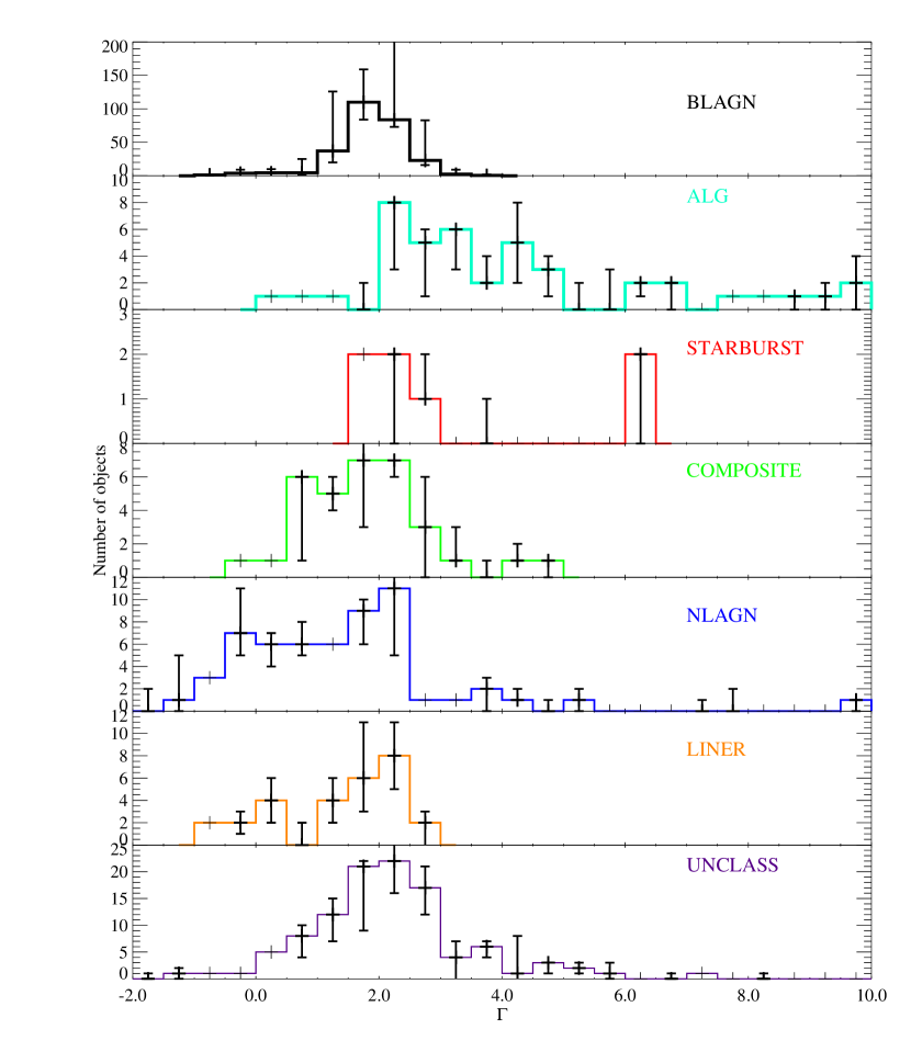
Figure 2.— The distribution of $\Gamma$ for the log $L_{X}$ $>$42 sample, separated into subclasses based on optical spectroscopic classification. Error bars show the Poisson errors on the number sources in each bin. From top to bottom: broad-line AGN, absorption line galaxies (ALG), star-forming objects, composite objects, narrow-line AGN and unclassified objects.

To enlarge our samples of galaxy nuclei of all spectral types, we also explored an emission-line classification based on only the [O III]/H$\beta$ vs. [N II]/H$\alpha$ diagram, i.e., a 4-line classification method, for the X-ray detected sources. The emission line galaxy samples comprise thus all objects showing at least 2$\sigma$ confidence in the line flux measurements of these four lines only. The delimitation criteria of star-forming and composite objects remain unchanged, while Seyferts and LINERs are defined to be all objects situated above the Kewley et al. (2006) separation line, and with [O III]/H$\beta$ greater and less than 3 respectively. Throughout the analysis presented in this paper we will call NLAGN the objects classified as Seyferts via the BPT diagrams.

4. BOLOMETRIC LUMINOSITIES

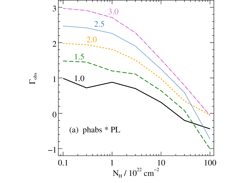
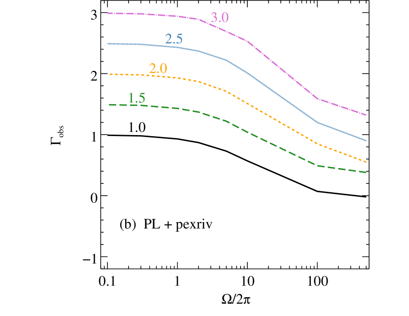
Figure 3.— Observed X-ray photon index as a function of the absorption column density (LEFT: XSPEC model phabs $\times$ power law) and reflection amplitude (RIGHT: XSPEC model pexriv with ionization parameter 10). The intrinsic X-ray photon index varies between 1.0 and 3.0. X-ray power law spectra absorbed with N_H$>$10²³ cm^-2, and reflection dominated X-ray spectra with $\Omega$/2$\pi$ $>$ 5-10 result in dramatically decreased observed X-ray photon index, reaching negative values for N_H$>$ few times 10²³ cm^-2.

To estimate bolometric luminosities and check for the presence of starburst and/or AGN activity in our sample, we fit the X-ray-to-radio fluxes with various empirical SEDs of well-observed sources as described in Trichas et al. (2012). We have used a total of 41 such templates, 16 from Ruiz et al (2010) and Trichas et al (2012) and 25 from Polletta et al. (2006). We have adopted the model described in Ruiz et al. (2010) and Trichas et al. (2012) which fits all SEDs using a $\chi$² minimization technique within the fitting tool Sherpa (Freeman et al. 2001). Our fitting allows for two additive components, using any possible combination of AGN, starburst and galaxy templates. The SEDs are built and fitted in the rest-frame. For each galaxy, we have chosen the fit with the lowest reduced $\chi$² as our best fit model. Fractions of AGN, starburst and galaxy contributions are derived from the SED fitting normalizations as these are derived from Ruiz et al. (2010) model,

$${F_{\nu}=F_{Bol}~{}(\alpha~{}u_{\nu}^{i}~{}+~{}(1-\alpha)~{}u_{\nu}^{j})}$$ (1)

where $i$ and $j$ can be AGN, starburst or galaxy, F_Bol is the total bolometric flux, $\alpha$ is the relative contribution of the i component to F_Bol , F_ν is the total flux at frequency $\nu$, while $u_{\nu}^{i}$ and $u_{\nu}^{i}$ are the normalized i and j templates.

4.1. Comparison between SED fitting and optical spectroscopic classification

Among the 617 sources in our sample, 203 are broad-line AGN (BLAGN) and 414 are narrow-emission/absorption line galaxies. The majority of the sources are best fitted with a combination of templates however of the 203 BLAGN, in 168 (82$\%$) the dominant contribution is fitted with one of our QSO templates, in 34 (17$\%$) with one of our NLAGN templates and in only 2 ($<$1$\%$) with a non-AGN template. Of the 414 narrow emission or absorption line galaxies, in 399 (96$\%$) the dominant contribution is fitted with one of our NELG/ALG templates with only 15 (4$\%$) being fit with a BLAGN template.

Of the 414 narrow-emission/absorption line galaxies based on spectral features and reliable emission line diagnostics, were possible, we have 63 passives, 39 H$\,II$s, 77 transition objects, 130 Seyferts and 38 LINERs. In 84$\%$ of the passives the dominant contribution is fitted by one of our elliptical templates, in 100% of the H$\,II$s with one of the star-forming templates and in 98% of the Seyferts with one of our Seyfert templates. All (100%) of the transition objects require a combination of AGN and star-forming templates to fit observed photometry. In the case of LINERs, the dominant contribution is best fitted with a Seyfert, passive, or star-forming template in 37$\%$, 50$\%$ and 13$\%$ of the cases respectively.

Based on the above we can securely claim that the agreement of our SED fitting with optical spectroscopic classification is excellent for all types of these objects.

5. X-ray Spectral Fitting

Based on the method used in Trichas et al. 2012, we perform X-ray spectral fitting to all X-ray sources in our sample, using the CIAO Sherpa tool. For each source we fit three power-law models that all contain an appropriate neutral Galactic absorption component frozen at the 21 cm value: (1) photon index $\Gamma$, with no intrinsic absorption component (model “PL”) (2) an intrinsic absorber with neutral column ${N_{H}^{intr}}$ at the source redshift, with photon index frozen at $\Gamma=1.8$ (model “PLfix”). Allowed fit ranges are $-1.5<\Gamma<3.5$ for PL and $10^{18}<{N_{H}^{intr}}<10^{25}$ for PLfix. (3) a two-parameter absorbed power-law where both $\Gamma$ and the ${N_{H}^{intr}}$ are free to vary within the above ranges while ${N_{H}^{Gal}}$ is fixed (model “PL_abs”). All models are fit to the ungrouped data using Cash statistics (Cash, 1979). The latter model, PL_abs, is our default.

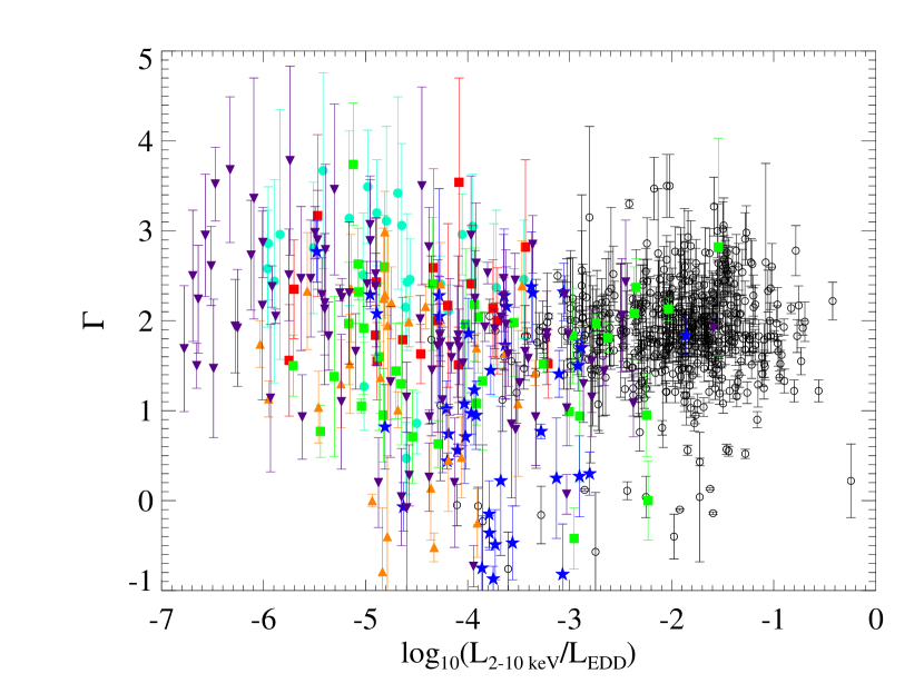
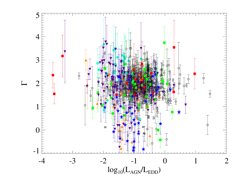
Figure 4.— LEFT: $\Gamma$ - L_X(2-10keV)/L_Edd relation for all z$<$0.4 CSC/SDSS AGN/Galaxies and ChaMP high-z QSOs (Trichas et al. 2012) with $\Gamma_{max}$ - $\Gamma_{min}$$\leq$3 and minimum net counts of 20. Symbols are as described in Figure 1. RIGHT: $\Gamma$ - L_AGN/L_Edd relation for all z$<$0.4 CSC/SDSS AGN/Galaxies and ChaMP high-z QSOs (Trichas et al. 2012) with $\Gamma_{max}$ - $\Gamma_{min}$$\leq$3 and minimum net counts of 20. L_AGN is the bolometric AGN luminosity as calculated by Trichas et al. (2012) SED template fitting method.

As discussed in Trichas et al. (2012), the best-fit $\Gamma$ from our default model is not correlated with ${N_{H}^{intr}}$, which illustrates that these parameters are fit with relative independence even in low count sources. Furthermore, the best-fit $\Gamma$ in the default PL_abs model correlates well with that from the PL model for the majority of sources; the (median difference is 15% of the median uncertainty).

A potentially useful Figure 2 shows the distribution of $\Gamma$ for all sources with log $L_{X}$ $>$42 divided by optical spectroscopic class. As the X-ray emission in all these sources is predominantly coming from an AGN, the peak of its distribution appears to be at around $\Gamma$=2 as expected. This indicates that for luminous X-ray sources $\Gamma$ is not likely to be severely affected by stellar X-ray emission from the host. However, although the peak of each distribution is the same, the histogram shape appears to change as we move to the type 2 spectral type sources corresponding to lower luminosity, or weaker accretion, e.g., LINERs and Composites, that could account for different inclinations, and thus dustier circumnuclear regions and not necessarily for intrinsically hard ionizing continua, for which there is a strong hard tail in the $\Gamma$ distribution and a sharp drop above $\Gamma$=2. For ALG, the mode is at $\Gamma\sim 2.0$, confirming that these sources contain a powerful AGN, but a a soft tail also indicates the likelihood of either a different accretion mode, or perhaps contributions from softer emission components such as thermal bremsstrahlung from a hot interstellar medium, or even from circumgalactic hot gas, e.g., from the remnants of a ’fossil’ galaxy group. These sources are typical examples of X-ray Bright Optically Inactive Galaxies (XBONG) (Comastri et al. 2002). Four possible explanations have been proposed for the nature of these objects (e.g. Green et al. 2004): a ^′′buried^′′ AGN (Comastri et al. 2002), a low luminosity AGN (Severgnini et al. 2003), a BL Lac object (Yuan $\&$ Narayan 2004) and galactic scale obscuration (Rigby et al. 2006; Civano et al. 2007). The unclassified objects appear to follow a similar distribution to the dustier objects. This is expected as these are sources with very strong narrow emission lines which we fail to classify because of the issues discussed in Section 3.

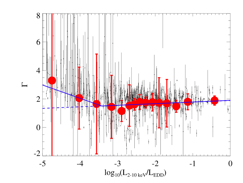
Figure 5.— $\Gamma$, as a function of $L_{\rm 2-10keV}/L_{\rm edd}$ ratio for all sources in our sample. Black dots represent the individual sources with their $\Gamma$ errors. The red circles represent the weighted mean values in each bin. The sample has been divided into 15 bins with the same number of sources per bin. The uncertainties shown represent the variance in the bin. The blue lines show the best fit with a broken linear model (solid line) and a single linear model (dashed line).

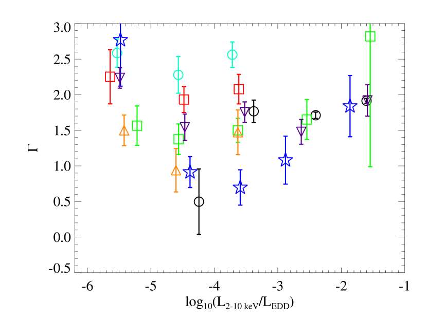
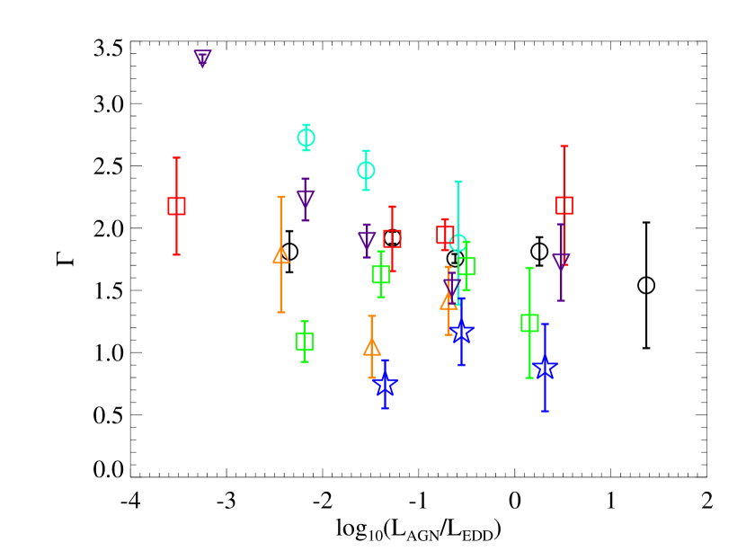
Figure 6.— Average $\Gamma$ per bin of $\Delta$log$\,\,L/L_{\rm Edd}$=1 for each spectral type of objects. Colors and shapes are the same as Figure 4. LEFT: We have used the Eddington luminosity calculation with hard X-ray luminosity. RIGHT: Eddington ratio using the SED-derived bolometric AGN luminosity.

For objects with sufficient X-ray counts and for which none of the aforementioned models provide a satisfactory fit, multiple additional models could be fitted to account for other possible sources of X-ray emission, e.g., from the hot ISM, or a separate power-law component from X-ray binary populations. In fact, most of our sources have too few counts to warrant such detailed fitting.

Objects for which we find very low (or even negative) $\Gamma$ could be heavily intrinsically absorbed, in which case we observe primarily the reflected component. Modeling this in the 2-10 keV band with a power law would result in very hard apparently unphysical slopes. We show a simple simulation in Figure 3 to illustrate. We used two very simple XSPEC (Arnaud et al. 1996) models (1) phabs*PL and (2) PL+pexriv (with ionization parameter 10, so effectively reflection from neutral matter). The different contours show how the measured $\Gamma$ depends on the (1) absorbing column $N_{H}$ and (2) strength of reflection $\Omega/2\pi$, for intrinsic $\Gamma$ = 1.0, 1.5, 2.0, 2.5, 3.0. These plots illustrate that negative observed values of $\Gamma$ more likely correspond to the absorption case, at least in this very simple approach.

To clarify this issue, deep X-ray exposures, preferably with hard X-ray response extending above $\sim$8 keV are required to allow more detailed X-ray spectral analysis. Additionally, we might expect that such objects show less X-ray variability, since intrinsic variability would be averaged by the reflection process (Sobolewska $\&$ Done 2007).

All multi-wavelength data are given in an online table available from the journal. A subsample of this table is given as an example in Table 1.

6. $\Gamma$ - L/L_Edd relation for z$<$0.4 AGN/Galaxies

The relation between the X-ray photon index $\Gamma$ and the Eddington ratio for the entire SDSS/CSC sample of sources with optical spectra at z$<$0.4 is illustrated in Figure 4. X-ray luminosity has been calculated using the method described in Green et al. (2011) and bolometric luminosities have been calculated as described in Section 4. Figure 4 shows 484 sources with minimum net counts of 20 and where the difference between the upper and lower 90% confidence limits to $\Gamma$ ($\Gamma_{\rm max}-\Gamma_{\rm min}$) $\leq$3. These selection criteria are applied in order to include only sources that have meaningful X-ray spectral fits (Section 5). Different colors in Figure 4 represent the different spectral classes as shown in Figure 1. To allow sampling of higher accretion rates, the BLAGN sample in Figure 4 contains both CSC/SDSS z$<0.4$ QSOs and high redshift QSOs from the Chandra Multwiavelength Project (ChaMP) spectroscopic sample of Trichas et al. (2012).

We have estimated the bolometric luminosity of the AGN component for every SED in our sample for the purpose of testing whether its relationship with Eddington ratio might reveal a more tightly correlated trend, since the full AGN power is better estimated thereby. However, the two panels in Figure 4, which differ only in the usage of $L_{X}$ vs L_AGN, reveal that $L_{X}$/L_Edd results in a stronger trend, more easily separating the AGN-dominated objects at higher Eddington ratio.

We first suspected that the use of $\Gamma$ in the calculation of $L_{X}$ itself might cause part of the correlation. We therefore examined plots instead using a fixed $\Gamma$=1.9 to calculate $L_{X}$, and note no phenomenological difference (the change is $\buildrel<\over{\sim}$0.1 in the Eddington ratio for $>90\%$ of the objects). There may be a failure of SED fitting to assess correctly bolometric luminosities in cases where only a limited number of photometric bands is available, or the reasons may be physical; the relative optical-infrared contribution to $L_{\rm Bol}$ may be larger especially for star-forming NELGs or ALGs. We certainly expect - and we believe these plots confirm - that while $L_{X}$ may provide an incomplete measure of AGN power, it is the purest such measure available for a sample of this type.

To test whether we truly see an inflection point similarly to what is observed in XRB we have selected all our objects with a clear indication of AGN activity as identified in X-rays, namely sources with log $L_{X}$ $>$42. We have then split them in bins with equal number of sources per bin and calculated average $\Gamma$ and $L_{X}$/L_Edd values. An ordinary least squares bisector method for linear regression was used for the fitting. Figure 5 shows a very similar feature to that noted by Wu $\&$ Gu (2008). The inflection point found by the latter is at the same $L_{X}$/L_Edd value as in our Figure 5 for AGN.

A comparison between the $\chi$² values of the broken linear fit versus a single linear fit indicates that the broken linear fit is always a better fit. The latter as well as the inflection point value are independent from the number of bins used for the fitting. To test the statistical significance of the $\chi$² results between broken and single linear fits, we have performed the p-value test (e.g. Sturrock $\&$ Scargle, 2009) that compares the likelihood ratios of fits done with a null hypothesis (i.e. single linear fit) and those with an alternative statistic (i.e. broken linear fit) using data simulated with Poisson noise. We have run the test using 20,000 simulations. The null hypothesis can be rejected if the p-value $\leq$ 0.05 which is the default significance level for this kind of test. For our sample p-value $<$ 0.004 every time we run the test suggesting that the broken liner fit with a single inflection point is at 5$\%$ significance level, always a better solution to the single linear fit.

In Figure 6 we use the exact same selection sample as in Figure 2 to plot the average $\Gamma$ per bin of log$\,\,L/L_{\rm Edd}$=1 separately for each spectral type. Number of objects differ per bin which might affect the error calculation. While in the case of the L_AGN/L_Edd the points show no trend, in the case of $L_{X}$/L_Edd it is obvious that narrow-line AGN show a simila break to the one observed in X-ray binaries (e.g. Wu $\&$ Gu 2008; Sobolewksa et al. 2011). For other spectral types, no clear results can be drawn as the populations do not cover the entire range of L/L_Edd.

A closer inspection of each of the spectral types for the entire CSC/SDSS spectroscopic z$<$0.4 population in Figure 6 indicates that the subsample that exhibits the strongest such trend is the population of NLAGN (blue stars). We have tested whether there is an underlying extrinsic cause for this strong trend for NLAGN mainly by checking how the difference in column densities and star-formation properties might affect it. Figure 7 (left) shows these trends for NLAGN with $log$ $L_{X(2-10keV)}>42$. Star-formation values (the mean luminosity attributed to the best-fit star-forming template components) have been retrieved by our SED fitting method. We might suspect that a significant contribution from star formation might artificially soften our measured $\Gamma$. However, the star-formation contribution from the host remains fairly constant as a function of $L_{X}$/L_Edd and in fact, the strongest contribution is where measured mean $\Gamma$ is hardest, so star-formation is not likely to affect the trend significantly. Another extrinsic effect might be that the hardest measured $\Gamma$ values around the inflection point could be caused by larger, yet poorly-fit individual column densities, and/or some inverse correlation between the fit parameters $\Gamma$ and N${}_{H}^{intr}$  as they compete to model the observed spectral shape. Figure 7 (right) shows some marginal evidence that this could be a problem, because the hardest bin has the lowest mean N${}_{H}^{intr}$.

Figure 7.— LEFT: Average $\Gamma$ versus Eddington ratio for all narrow-line AGN with log $L_{X}$ $>$42 erg/sec. The stars represent the mean $\Gamma$ values in each Eddington ratio bin. Each bin contains the same number of sources. Error bars are the 1$\sigma$ $\Gamma$ error in each bin. The mean starburst luminosity is given next of each star in erg/sec. RIGHT: Average $\Gamma$ versus Eddington ratio for all narrow-line AGN with log $L_{X}$ $>$42. The stars represent the mean $\Gamma$ values in each Eddington ratio bin. Each bin contains the same number of sources. Error bars are the 1$\sigma$ $\Gamma$ error in each bin. The mean number of N_H is given next of each star.

We retested our fits to the relations $\Gamma$, as a function of $L_{\rm 2-10keV}/L_{\rm edd}$ for all sources in our sample after excluding all spectroscopically identified narrow-line AGN, and find no significant difference.

7. The $\alpha_{\rm ox}$ - L/L_Edd relation

Trends of $\alpha_{\rm ox}$  vs. Eddington ratio for AGN are expected to be analogous to the SED variations of XRBs as well (e.g. Sobolewska et al. 2011). Indeed, such $\alpha_{\rm ox}$  trends may be expected to be stronger than those with $\Gamma$, because the optical/UV emission tracks disk emission with greater separation from AGN X-ray emission, which is more strongly dominated by the corona.

Figure 8 shows the average values of $\alpha_{\rm ox}$  vs $L_{X}$/L_Edd ratio for our sample of sources with log $L_{X}$ $>$42 (open black circles). Binned average points from Grupe et al (2010; open blue triangles) and Lusso et al (2010; filled red circles) are shown for comparison. We estimate the 2-10 keV luminosity from the tablulated 0.–2 keV luminosities in Grupe et al. (2010) by simply assuming $\Gamma=1.9$. The 150 XMM-COSMOS BLAGN with M_BH estimates from Lusso et al (2010) span a wide range of redshifts (0.2$<$z$<$4.25) and X-ray luminosities between 42.4$<$log L${}_{(2-10\,keV)}<$45.1. However our study extends the relationship down as far as log $L_{X}$/L_Edd$<$-4. At the high Eddington ratio end, there is a suggestion of an upturn, as expected from the scaling experiments of Sobolewska et al. (2011). However, the upturn is based on a small number of points from Grupe et al. (2010), and are suspect in any case, because of the large uncertainties visible, and because log $L_{X}$/L_Edd exceeds unity.

Since both referenced papers studied Eddington ratios using estimates of bolometric luminosity, we also compare using our $L_{\rm AGN}$ estimate from SED fitting. Here we see evidence of a consistently positive trend. The Grupe et al. (2010) points are again offset in the sense of being either X-ray bright, or perhaps more likely suffering from underestimated Eddington luminosities.

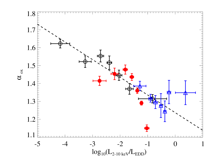
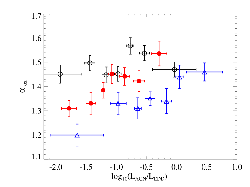
Figure 8.— Average values of $\alpha_{\rm ox}$ vs $L_{X}/L_{\rm Edd}$ ratio for our entire sample with log $L_{X}$ $>$42 erg/sec (open black circles). Each bin contains the same number of sources. The best-fit OLS Y(X) regression plotted for our sample alone (dashed line). We also show the sample of Grupe et al. (2010; blue triangles), and of Lusso et al. (2010; filled red circles), binned similarly. The apparently super-Eddington points from Grupe et al. (2010) are probably influenced by uncertainties in the use of FWHM(H$\beta$) to calculate M_BH for these objects.

For comparison to Figure 8 (top), we offer Figure 9, based on the simulations of Sobolewska et al. (2011). Here, the observed SED evolution of the XRB GRO J1655−40 was scaled to a simulated population (BH mass distribution) of AGN, by stretching and scaling a (3 vs. 20 keV) disc-to-Componization index $\alpha^{\prime}$ to an AGN’s analogous $\alpha_{\rm ox}$ (between 2500Å  and 2 keV). The exact values displayed are not of particular interest, because the simulations convert expected analogous trends for AGN extrapolating from the behavior in outburst of one particular X-ray binary However, the overall trends are instructive.

In Figure 8 (top), the simulated AGN located on the upper branch (circles) correspond to the soft state XRBs, with ultrasoft states located in the upper left corner. All points are shaded with the bolometric correction that should be applied to the 2-10 keV luminosity to get $L_{\rm Bol}$. The ultrasoft states have the largest bolometric correction because they are dominated by the accretion disk component with only marginal contribution from the power-law tail. These points most probably correspond to X-ray weak AGN (.e.,g as indicated with a red diamond in Fig 3 of Vasudevan & Fabian (2007).

The simulated AGN sitting on the lower branch (triangles) correspond to hard state XRBs. In general $\alpha_{\rm ox}$  is lower in the hard state than in the soft state for comparable $L_{X}$/L_Edd due to less vigorous accretion disk emission. It is for these hard states that we see not only a convincing anti-correlation of $\alpha_{\rm ox}$  with $L_{X}$/L_Edd, but even an upturn just shy of the highest Eddington ratios. For the soft state (disc-dominated) AGN, changes in $L_{X}$ do not significantly change the $L_{\rm Bol}$, which results in the varying bolometric correction seen at the top, and the poor correlation between $L_{\rm X}/L_{\rm Edd}$ and $L_{\rm Bol}/L_{\rm Edd}$ seen in Figure 8(bottom).

We believe that the AGN plotted in Figure 8 may correspond to the soft state branch and bright (in terms of $L_{\rm Bol}/L_{\rm Edd}$) part of the hard state branch, and that is why the turnover is weak in our observed sample. This is confirmed in the lower panel of Figure 8, where $L_{\rm AGN}/L_{\rm Edd}$ is never lower than $\sim-2$.

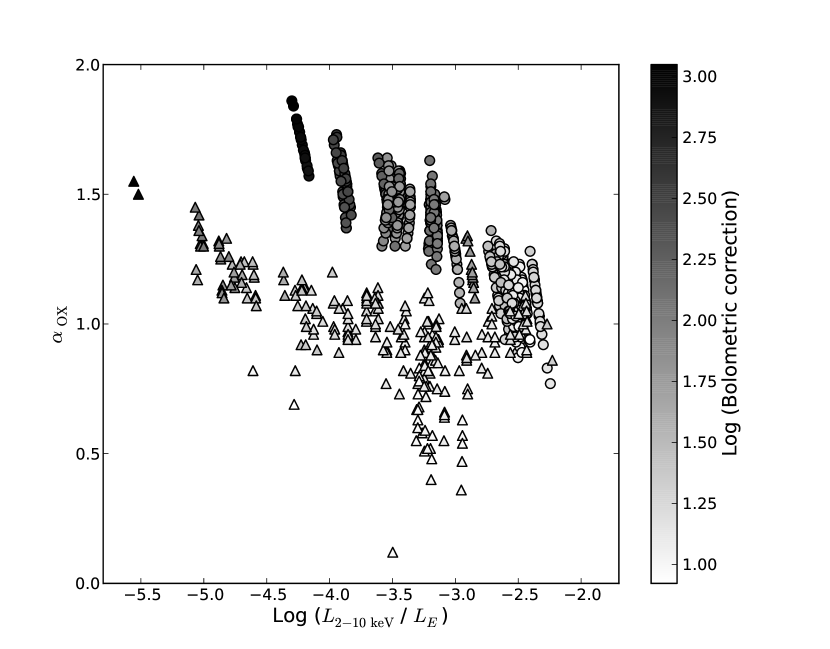
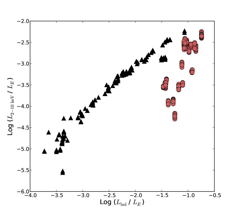
Figure 9.— Simulations of the X-ray binary GRO J1655−40, scaled to a simulated AGN population as described in the text. Circles show the AGN-equivalent soft state, and triangles hard state. The bolometric correction from $L_{X}$ is shown as a grayscale (top). In the bottom panel, Eddington ratios are plotted against one another using $L_{X}$ and $L_{\rm Bol}$. The soft state analogs (orange circles) show little correlation, because their SEDs are so strongly dominated by disc (optical/UV) emission.

8. X-ray/Emission Line Relationships

Observed relationships between emission line and X-ray luminosities can be quite useful for predicting from optical ground-based spectroscopy the (more expensive) X-ray exposure times required to achieve a desired S/N. Such trends can also help us understand the physical relationship between broad vs. narrow line emission and accretion power.

Panessa et al. (2006) studied various correlations between X-ray and H$\alpha$, [O III] line luminosities, from 60 “mixed” Seyferts, both narrow and broad lined Seyferts, in the Palomar survey of nearby ($B_{T}<12.5$) galaxies (Ho, Filippenko, & Sargent 1997) and a sample of PG quasars from Alonso-Herrero et al. (1997). Our sample extends to larger redshifts and X-ray luminosities that may be better-matched to typical X-ray AGN studies.

Figure 10 (left) shows the logarithmic 2-10 keV luminosity versus logarithmic H$\alpha$ luminosity. The black solid line shows the best linear (OLS) regression line

$${\log L_{X}=(1.02\pm 0.03)\log L_{H\alpha}-(1.18\pm 1.25)}$$ (2)

obtained by fitting our BLAGN sample (open black circles). The green solid line (with slope $0.95\pm 0.07$ and intercept $-3.87\pm 2.76$) represents the best-fit linear regression line from Panessa et al. (2006) that they obtained by fitting the total sample of Seyfert-1 galaxies and low redshift (PG) quasars. While the difference in normalization is most apparent to the eye, the values are consistent within the errors.

Dashed blue and green lines represent the best fit to both broad and narrow-line AGN for our sample and Panessa et al. 2006 respectively. Our fit is given by

$${\log L_{X}=(0.66\pm 0.03)\log L_{H\alpha}-(1.32\pm 1.08)}$$ (3)

where Panessa et al. found slope $1.06\pm 0.04$ and intercept $-1.14\pm 1.78$. The offset between the samples is reminiscent of that presented by Green, Anderson & Ward (1992) in contrasting the 60$\mu$m and X-ray emission between narrow- and broad- line galaxies. Both H$\alpha$ and (IRAS) 60$\mu$m luminosity is known to correlate strongly with star-formation power, which may be relatively strong in the nearby sample.

In the case of the logarithmic 2-10 keV luminosity versus logarithmic [O III] luminosity for both BLAGN and NLAGN the agreement is generally excellent. We find

$${\log L_{X}=(1.26\pm 0.04)\log L_{[OIII]}-(7.36\pm 1.80)}$$ (4)

where the Panessa et al 2006 relationship is fit with slope $1.22\pm 0.06$ and intercept $-7.34\pm 2.53$. We suggest that since [O III] is a higher ionization line, it tracks X-ray emission more accurately across a wider range of accretion power, especially where the relative contribution from star formation may be appreciable.

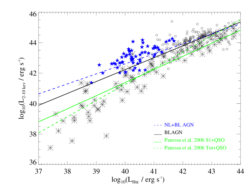
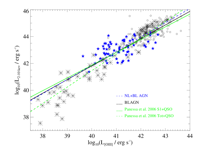
Figure 10.— Logarithmic 2-10 keV luminosity versus logarithmic emission line luminosity. LEFT: For H$\alpha$ emission. Open circles represent our BLAGN, blue filled stars are our NLAGN, and asterisks are Seyfert galaxies and low redshift QSOs from Ward et al. (1988) used in Panessa et al. (2006). The black lines show the best fit (OLS) linear regression from our sample for BLAGN and NLAGN (solid) or just BLAGN (dashed). The green solid line represents the best fit linear regression line from Panessa et al. (2006) for their full sample. RIGHT: For [O III] emission. Same symbols as at left. The black lines show the best fit (OLS) linear regression from our sample for BLAGN and NLAGN (solid) or just BLAGN (dashed). The green lines represents the best fit linear regression line from Panessa et al. (2006) for Seyfert galaxies (solid) and for their full sample (dashed), consisting of bright type 1 Seyferts (Mulchaey et al. 1994) and a sample of PG quasars (Alonso-Herrero et al. 1997).

9. Summary

We confirm a significant V-shaped trend across a large sample of X-ray detected galaxies and AGN in the plane of X-ray spectral hardness and Eddington ratio, when expressed as $L_{X}$/L_Edd. The dispersion in the trend is significant for a variety of reasons beyond intrinsic dispersion in the accretion states of AGN. The X-ray spectral fits are often marginal due to poor photon statistics, and are generally unable to model the known X-ray spectral complexity of real AGN, including possible warm absorption, reflection components, etc. We further acknowledge the rather significant uncertainties involved in estimation of the Eddington luminosities from the $M_{\rm BH}$ - $\sigma$ relation (for narrow emission and absorption line galaxies) and the FWHM(H$\beta$)/$L_{\rm 5100\AA}$ method (for BLAGN).

Nevertheless, despite the intrinsic dispersion and measurement uncertainties, we find on average a V-shaped correlation between X-ray spectral hardness and Eddington ratio that is similar both in shape and in the location of the inflection point, to analogous trends seen in X-ray binary systems as they vary. When separating AGN by (optical spectroscopic emission line) classification, the strongest trend is shown by the NLAGN. A necessarily rather simple analysis shows no evidence that this apparent trend is either strengthened or caused by the contributions of softer stellar emission components or hardening due to intrinsic absorption. We also test for a predicted V-shaped trend of X-ray to optical spectral slope $\alpha_{\rm ox}$  with Eddington ratio, but find only a monotonic relationship whereby BLAGN become relatively more X-ray bright (weak) compared to Eddington ratio expressed in terms of X-ray (total AGN) luminosity.

Table 1Sample of our full online catalog

SDSS J name	redshift	Class	log $M_{\rm BH}$	net Counts	$\Gamma$	${\rm N}^{intr}_{H}$	F(2-8 keV)	log $L_{X}$/LEdd	$L_{\rm AGN}$
J122137.2+295701	0.17	5	7.96$\pm 0.40$	26	1.84${}^{+0.88}_{-0.58}$	21.04$\pm 0.52$	13.94${}^{+6.37}_{-6.36}$	-3.09	45.02
J123614.5+255022	0.18	5	7.86$\pm 0.42$	30	2.91${}^{+1.66}_{-0.84}$	22.80$\pm 0.22$	11.53${}^{+4.46}_{-4.43}$	-3.01	45.09
J112314.9+431208	0.08	3	7.55$\pm 0.37$	123	1.86${}^{+0.39}_{-0.36}$	21.94$\pm 0.37$	33.33${}^{+3.21}_{-3.25}$	-2.99	44.08
J153600.9+162839	0.38	6	7.83$\pm 0.22$	69	2.13${}^{+0.24}_{-0.40}$	21.00$\pm 0.52$	139.4${}^{+29.8}_{-30.0}$	-1.13	45.51
J120100.1+133127	0.20	6	7.55$\pm 0.30$	68	1.68${}^{+0.54}_{-0.47}$	21.77$\pm 0.03$	203.5${}^{+27.6}_{-28.0}$	-1.32	44.99
J141652.9+104826	0.02	5	9.24$\pm 0.54$	200	2.05${}^{+0.08}_{-0.08}$	20.60$\pm 0.30$	240.5${}^{+5.6}_{-5.4}$	-4.88	45.23
J090105.2+290146	0.19	3	8.14$\pm 0.34$	67	2.16${}^{+0.44}_{-0.41}$	21.26$\pm 0.03$	43.95${}^{+5.70}_{-5.63}$	-2.62	45.11
J122959.4+133105	0.10	3	7.11$\pm 0.30$	228	0.3${}^{+0.24}_{-0.22}$	21.28$\pm 0.15$	119.7${}^{+8.2}_{-8.2}$	-1.80	44.39
J122843.5+132556	0.25	0	9.00$\pm 0.31$	64	2.37${}^{+0.86}_{-0.67}$	21.25$\pm 0.15$	137.9${}^{+60.3}_{-59.61}$	-2.72	45.30
J141531.4+113157	0.26	6	7.81$\pm 0.29$	293	1.74${}^{+0.05}_{-0.05}$	20.48$\pm 0.01$	229.9${}^{+4.4}_{-4.3}$	-1.29	45.23
J111809.9+074653	0.04	2	7.26$\pm 0.49$	29	1.97${}^{+0.68}_{-0.54}$	20.90$\pm 0.35$	4.38${}^{+0.73}_{-0.73}$	-4.17	44.42
J121531.2-003710	0.35	0	9.49$\pm 0.22$	21	3.67${}^{+1.09}_{-0.87}$	21.94$\pm 0.15$	4.07${}^{+1.67}_{-1.64}$	-4.42	45.64
J145241.4+335058	0.19	6	7.92$\pm 0.30$	43	1.41${}^{+1.05}_{-0.86}$	22.73$\pm 0.14$	53.84${}^{+8.66}_{-8.57}$	-2.33	44.96
J102451.2+470738	0.14	5	7.75$\pm 0.38$	57	2.25${}^{+0.53}_{-0.48}$	21.23$\pm 0.01$	17.73${}^{+2.56}_{-2.54}$	-2.93	44.74
J082332.6+212017	0.02	1	7.64$\pm 0.42$	53	2.35${}^{+0.55}_{-0.50}$	21.49$\pm 0.13$	17.13${}^{+2.58}_{-2.60}$	-4.70	42.14
J141910.3+525151	0.08	2	7.27$\pm 0.46$	43	1.44${}^{+0.53}_{-0.40}$	20.95$\pm 0.55$	3.28${}^{+0.57}_{-0.56}$	-3.70	44.81
J011544.8+001400	0.04	3	6.38$\pm 0.50$	350	1.7${}^{+0.17}_{-0.17}$	20.90$\pm 0.01$	100.10${}^{+5.7}_{-5.73}$	-1.89	44.26
J011522.1+001518	0.39	5	9.24$\pm 0.25$	386	1.31${}^{+0.19}_{-0.19}$	22.25$\pm 0.30$	147.70${}^{+7.80}_{-7.70}$	-2.49	45.69
J082001.8+212107	0.08	1	6.53$\pm 0.42$	29	2.82${}^{+0.97}_{-0.48}$	20.30$\pm 0.08$	11.03${}^{+2.23}_{-2.21}$	-2.43	43.93
J020925.1+002356	0.06	2	6.76$\pm 0.44$	40	1.83${}^{+0.53}_{-0.34}$	20.30$\pm 0.01$	99.61${}^{+18.99}_{-18.80}$	-1.97	44.39
J153311.3-004523	0.15	3	8.01$\pm 0.28$	37	1.92${}^{+1.27}_{-1.13}$	22.93$\pm 0.28$	164.8${}^{+28.0}_{-28.4}$	-2.16	44.82
J002253.2+001659	0.21	5	7.63$\pm 0.34$	150	1.03${}^{+0.42}_{-0.40}$	22.55$\pm 0.52$	43.03${}^{+3.69}_{-3.66}$	-2.03	44.79
J155627.6+241800	0.12	2	7.38$\pm 0.37$	94	0.94${}^{+0.73}_{-0.67}$	22.61$\pm 0.30$	119.1${}^{+15.6}_{-15.5}$	-1.90	44.66
J103515.6+393909	0.11	3	6.24$\pm 0.34$	33	1.7${}^{+1.23}_{-1.01}$	22.83$\pm 0.23$	109.2${}^{+20.2}_{-19.08}$	-0.89	44.27

References

- [1] Aird, J., et al., 2010, MNRAS, 401, 2531
- [2] Alonso-Herrero A., 1997, MNRAS, 288, 977
- [3] Arnaud K., et al., 1996, ApJ, 462, 75
- [4] Baldwin J., et al., 1981, PASP, 93, 5
- [5] Becker R. et al., 1995, ApJ, 450, 559
- [6] Cash W., 1979, ApJ, 228, 939
- [7] Civano F., et al., 2007, AA, 476, 1223
- [8] Comastri A., et al., 2002, ApJ, 571, 771
- [9] Constantin A. Vogeley M., 2006, ApJ, 650, 727
- [10] Constantin A., Hoyle F. Vogeley M., 2008, ApJ, 673, 715
- [11] Constantin A., et al., 2009, ApJ, 705, 1336
- [12] Croton, D., et al., 2006, MNRAS, 365, 11
- [13] Evans I., et al., 2010, ApJS, 189, 37
- [14] Fadda, D., et al., 2002, AA, 383, 838
- [15] Freeman P., et al., 2001, SPIE, 4477, 76
- [16] Graham A., et al., 2011, MNRAS, 412, 2211
- [17] Green P., et al., 1992, MNRAS, 254, 30
- [18] Green P., et al., 2004, ApJS, 150, 43
- [19] Green P., et al., 2011, ApJ, 743, 81
- [20] Greene J. Ho L., ApJ, 667, 131
- [21] Grupe D., et al., 2010, ApJS, 187, 64
- [22] Gultekin, K., et al., 2009, ApJ, 698, 198
- [23] Gultekin, K., et al., 2012, ApJ, 749, 129
- [24] Ho, L. C., Filippenko, A. V., & Sargent, W. L. W. 1997, ApJS, 112, 315
- [25] Hopkins, A. Beacom, J., 2006, ApJ, 651, 142
- [26] Hopkins, P., et al., 2006, ApJS, 163, 1
- [27] Kalfountzou E., et al., 2011, MNRAS, 413, 249
- [28] Kauffmann G. Heckman T., 2009, MNRAS, 397, 135
- [29] Kewley L., et al., 2006, MNRAS, 372, 961
- [30] Lawrence A., et al., 2007, MNRAS, 379, 1599
- [31] Lu H., et al., 2006, AJ, 131, 790
- [32] Lusso E, et al., 2010, AA, 512, 34
- [33] Miniutti G., et al., 2009, MNRAS, 394, 443
- [34] Morrissey P., et al., 2007, ApJS, 173, 682
- [35] Mulchaey J., et al., 1994, ApJ, 436, 586
- [36] Panessa F., et al., 2006, AA, 455, 173
- [37] Polletta M., et al., 2006, ApJ, 642, 673
- [38] Rigby J, et al., 2006, ApJ, 645, 115
- [39] Rots, A. et al., 2009, AAS, 21347203R
- [40] Ruiz A., et al., 2010, AA, 515, 99
- [41] Severgnini P., et al., 2003, AA, 406, 483
- [42] Shen Y., et al., 2011, ApJS, 194, 45
- [43] Skrutskie M., et al., 2006, AJ, 131, 1163
- [44] Sobolewska M. Done C., 2007, MNRAS, 374, 150
- [45] Sobolewska M., et al., 2011, MNRAS, 413, 2259
- [46] Sturrock P. Scargle J., 2009, ApJ, 706, 393
- [47] Taylor, M., 2005, ASPC, 347, 29
- [48] Trichas M., et al., 2009, MNRAS, 399, 663
- [49] Trichas M., et al., 2010, MNRAS, 405, 2243
- [50] Trichas M., et al., 2012, ApJS, 200, 17
- [51] Vasudevan, R. V., & Fabian, A. C. 2007,MNRAS, 381, 1235
- [52] Vestergaard M. Peterson B., 2006, ApJ, 641, 689
- [53] Ward M., et al., 1988, ApJ, 324, 767
- [54] Wright E., et al., 2010, AJ, 14O, 1868
- [55] Wu Q Gu M., 2008, ApJ, 682, 212
- [56] York D., et al., 2000, AJ, 120, 1579
- [57] Yuan, F., & Narayan, R, 2004, ApJ, 612, 724
- [58] Zhou H., et al., 2006, ApJS, 166, 128