On the existence of solutions to stochastic
quasi-variational inequality and complementarity problems

Abstract

Variational inequality problems allow for capturing an expansive class of problems, including convex optimization problems, convex Nash games and economic equilibrium problems, amongst others. Yet in most practical settings, such problems are complicated by uncertainty, motivating the examination of a stochastic generalization of the variational inequality problem and its extensions in which the components of the mapping contain expectations. When the associated sets are unbounded, ascertaining existence requires having access to analytical forms of the expectations. Naturally, in practical settings, such expressions are often difficult to derive, severely limiting the applicability of such an approach. Consequently, our goal lies in developing techniques that obviate the need for integration and our emphasis lies in developing tractable and verifiable sufficiency conditions for claiming existence. We begin by recapping almost-sure sufficiency conditions for stochastic variational inequality problems with single-valued maps provided in our prior work [42, 43] and provide extensions to multi-valued mappings. Next, we extend these statements to quasi-variational regimes where maps can be either single or set-valued. Finally, we refine the obtained results to accommodate stochastic complementarity problems where the maps are either general or co-coercive. The applicability of our results is demonstrated on practically occuring instances of stochastic quasi-variational inequality problems and stochastic complementarity problems, arising as nonsmooth generalized Nash-Cournot games and power markets, respectively.

1 Introduction

Motivation:

In deterministic regimes, a wealth of conditions exist for characterizing the solution sets of variational inequality, quasi-variational inequality and complementarity problems (cf. [8, 10, 27]), including sufficiency statements of existence and uniqueness of solutions as well as more refined conditions regarding the compactness and connectedness of solution sets and a breadth of sensitivity and stability questions. Importantly, the analytical verifiability of such conditions from problem primitives (such as the underlying map and the set) is essential to ensure the applicability of such schemes, as evidenced by the use of such conditions in analyzing a range of problems arising in power markets [19, 21, 50], communication networks [9, 38, 48, 56], structural analysis [39, 40], amongst others. The first instance of a stochastic variational inequality problem was presented by King and Rockafellar [26] in 1993 and the resulting stochastic variational inequality problem requires an $x\in X$ such that

$$(y-x)^{T}\mathbb{E}[G(x,\xi(\omega))]\,\geq\,0,\quad\forall y\,\in\,X,$$

where $X\subseteq\mathbb{R}^{n}$, $\xi:\Omega\to\mathbb{R}^{d}$, $G:X\times\mathbb{R}^{d}\to\mathbb{R}^{n}$, $\mathbb{E}[.]$ denotes the expectation in a component-wise sense, and $(\Omega,{\cal F},\mathbb{P})$ represents the probability space. In the decade that followed, there was relatively little effort on addressing analytical and computational challenges arising from such problems. But in the last ten years, there has been an immense interest in the solution of such stochastic variational inequality problems via Monte-Carlo sampling methods [22, 23, 28, 51]. But verifiable conditions for characterization of solution sets have proved to be relatively elusive given the presence of an integral (arising from the expectation) in the map. Despite the rich literature in deterministic settings, direct application of deterministic results to stochastic regimes is not straightforward and is complicated by several challenges: First, a direct application of such techniques on stochastic problems requires the availability of closed-form expressions of the expectations. Analytical expressions for expectation are not easy to derive even for single-valued problems with relatively simple continuous distributions. Second, any statement is closely tied to the distribution. Together, these barriers severely limit the generalizability of such an approach. To illustrate the complexity of the problem class under consideration, we consider a simple stochastic linear complementarity problem.

Example 1.

Consider the following stochastic linear complementarity problem:

$$0\leq x\perp\mathbb{E}\left[\begin{pmatrix}2&1\\ 1&2\end{pmatrix}x+\begin{pmatrix}-2+\omega_{1}\\ -4+\omega_{2}\end{pmatrix}\right]\geq 0.$$

Specifically, this can be cast as an affine stochastic variational inequality problem VI$(K,F)$ where

$$K\triangleq\mathbb{R}_{2}^{+}\mbox{ and }F(x)\triangleq\mathbb{E}[G(x;\omega)],\mbox{ where }G(x;\omega)\triangleq\left[\begin{pmatrix}2&1\\ 1&2\end{pmatrix}x+\begin{pmatrix}-2+\omega_{1}\\ -4+\omega_{2}\end{pmatrix}\right].$$

Consider two cases that pertain to either when the expectation is available in closed-form (a); or not (b):
(a) Expectation $\mathbb{E}[.]$ available in closed form: Suppose in this instance, $\omega$ is a random variable that takes values $\omega^{1}$ of $\omega^{2}$, given by the following:

$$\omega^{1}=\begin{pmatrix}1\\ 1\end{pmatrix}\mbox{ or }\omega^{2}=\begin{pmatrix}-1\\ -1\end{pmatrix}\mbox{ with probability }0.5.$$

Consequently, the stochastic variational inequality problem can be expressed as

$$0\leq x\perp\left[\begin{pmatrix}2&1\\ 1&2\end{pmatrix}x+\begin{pmatrix}-2\\ -4\end{pmatrix}\right]\geq 0.$$

In fact, this problem is a strongly monotone linear complementarity problem and admits a unique solution given by $x^{*}=(0,2).$ If one cannot ascertain monotonicity, a common approach lies in examining coercivity properties of the map; specifically, VI$(K,F)$ is solvable since there exists an $x^{\rm ref}\in K$ such that (cf. [10, Ch. 2])

$$\liminf_{\|x\|\to\infty,x\in K}F(x)^{T}(x-x^{\rm ref})>0.$$

(b) Expectation $\mathbb{E}[.]$ unavailable in closed-form: However, in many practical settings, closed-form expressions of the expectation are unavailable. Two possible avenues are available:

1. If $K$ is compact, under continuity of the expected value map, VI$(K,F)$ is solvable.

2. If there exists a single $x\in K$ that solves VI$(K,F(.;\omega))$ for almost every $\omega\in\Omega$, VI$(K,F)$ is solvable.

Clearly, if $K$ is a cone and (i) does not hold. Furthermore (ii) appears to be possible only for pathological examples and in this case, there does not exist a single $x$ that solves the scenario-based VI$(K,{G}(.;\omega))$ for every $\omega\in\Omega.$ Specifically, the unique solutions to VI$(K,G(.;\omega^{1}))$ and VI$(K,{G}(.;\omega^{2}))$ are $x(\omega^{1})=(0,3/2)$ and $x(\omega^{2})=(1/3,7/3),$ respectively and since $x(\omega^{1})\neq x(\omega^{2})$, avenue (ii) cannot be traversed. Consequently, neither of the obvious approaches can be adopted yet VI$(K,F)$ is indeed solvable with a solution given by $x^{*}=(0,2)$.

Consequently, unless the set is compact or the scenario-based VI is solvable by the same vector in an almost sure sense, ascertaining solvability of stochastic variational inequality problems for which the expectation is unavailable in closed form does not appear to be immediately possible through known techniques. In what could be seen as the first step in this direction, our prior work [43] examined the solvability of convex stochastic Nash games by analyzing the equilibrium conditions, compactly stated as a stochastic variational inequality problem. Specifically, this work relies on utilizing Lebesgue convergence theorems to develop integration-free sufficiency conditions that could effectively address stochastic variational inequality problems, with both single-valued and a subclass of multi-valued maps arising from nonsmooth Nash games. As a simple illustration of the avenue adopted, consider Example 1 again and assume that the expectation is unavailable in closed form, we examine whether the a.s. coercivity property holds (as presented in the next section). It can be easily seen that there exists an $x^{\rm ref}\in K$, namely $x^{\rm ref}\triangleq{\bf 0}$, such that

$$\liminf_{\|x\|\to\infty,x\in K}G(x;\omega)^{T}(x-x^{\rm ref})>0,\mbox{ for }{\omega=\omega^{1}\mbox{ and }\omega=\omega^{2}}.$$

It will be shown that satisfaction of this coercivity property in an almost-sure sense is sufficient for solvability. But such statements, as is natural with any first step, do not accommodate stochastic quasi-variational problems and can be refined significantly to accommodate complementarity problems. Moreover, they cannot accommodate multi-valued variational maps. The present work focuses on extending such sufficiency statements to quasi-variational inequality problems and complementarity problems and accommodate settings where the maps are multi-valued.

Contributions:

This paper provides amongst the first attempts to examine and characterize solutions for the class of stochastic quasi-variational inequality and complementarity problems when expectations are unavailable in closed form. Our contributions can briefly be summarized as follows:

(i) Stochastic quasi-variational inequality problems (SQVIs):

We begin by recapping our past integration-free statements for stochastic VIs that required the use of Lebesgue convergence theorems and variational analysis. Additionally, we provide extensions to regimes with multi-valued maps and specialize the conditions for settings with monotone maps and Cartesian sets. We then extend these conditions to stochastic quasi-variational inequality problems where in addition to a coercivity-like property, the set-valued mapping needs to satisfy continuity, apart from other “well-behavedness” properties to allow for concluding solvability. Finally, we extend the sufficiency conditions to accommodate multi-valued maps.

(ii) Stochastic complementarity problems (SCPs):

Solvability of complementarity problems over cones requires a significantly different tack. We show that analogous verifiable integration-free statements can be provided for stochastic complementarity problems. Refinements of such statements are also provided in the context of co-coercive maps.

(iii) Applications:

Naturally, the utility of any sufficiency conditions is based on its level of applicability. We describe two application problems. Of these, the first is a nonsmooth stochastic Nash-Cournot game which leads to an SQVI while the second is a stochastic equilibrium problem in power markets which can be recast as a stochastic complementarity problem. Importantly, both application settings are modeled with a relatively high level of fidelity.

Remark: Finally, we emphasize three points regarding the relevance and utility of the provided statements: (i) First, such techniques are of relevance when integration cannot be carried out easily and have less utility when sample spaces are finite; (ii) There are settings where alternate models for incorporating uncertainty have been developed [7, 35, 37]. Such models assume relevance when the interest lies in robust solutions. Naturally, an expected-value formulation has less merit in such settings and correspondingly, such robust approaches cannot capture risk-neutral decision-making. Consequently, the challenge of analyzing existence of this problem cannot be done away with by merely changing the formulation, since an alternate formulation may be inappropriate. (iii) Third, we present sufficiency conditions for solvability. Still, there are simple examples which can be constructed in finite (and more general) sample spaces where such conditions will not hold and yet solvability does hold. We believe that this does not diminish the importance of our results; in fact, this is not unlike other sufficiency conditions for variational inequality problems. For instance, we may construct examples where the coercivity of a map may not hold over the given set [10] but the variational inequality problem may be solvable. However, in our estimation, in some of the more practically occurring engineering-economic systems, such conditions do appear to hold, reinforcing the relevance of such techniques. In particular, we show such conditions find applicability in a class of risk-neutral and risk-averse stochastic Nash games in [42, 43]. In the present work, we show that such conditions can be employed for analyzing a class of stochastic generalized Nash-Cournot games with nonsmooth price functions as well as for a relatively more intricate networked power market in uncertain settings. Before proceeding to our results we provide a brief history of deterministic and stochastic variational inequalities.

Background and literature review:

The variational inequality problem provides a broad and unifying framework for the study of a range of mathematical problems including convex optimization problems, Nash games, fixed point problems, economic equilibrium problems and traffic equilibrium problems [10]. More generally, the concept of an equilibrium is central to the study of economic phenomena and engineered systems, prompting the use of the variational inequality problem [18]. Harker and Pang [16] provide an excellent survey of the rich mathematical theory, solution algorithms, and important applications in engineering and economics while a more comprehensive review of the analytical and algorithmic tools is provided in the recent two volume monograph by Facchinei and Pang [10].

Increasingly, the deterministic model proves inadequate when contending with models complicated by risk and uncertainty. Uncertainty in variational inequality problems has been considered in a breadth of application regimes, ranging from traffic equilibrium problems [7, 15], cognitive radio networks [30, 49], Nash games [43, 37], amongst others. Compared to the field of optimization, where stochastic programming [4, 52] and robust optimization [3] have provided but two avenues for accommodating uncertainty in static optimization problems, far less is currently available either from a theoretical or an algorithmic standpoint in the context of stochastic variational inequality problems. Much of the efforts in this regime have been largely restricted to Monte-Carlo sampling schemes [13, 22, 26, 29, 57, 28, 59, 41], and a recent broader survey paper on stochastic variational inequality problems and stochastic complementarity problems [32].

1.1 Formulations

To help explain the two main formulations for stochastic variational inequality problems found in literature - the expected value formulation and expected residual minimization formulation; we now define the variational inequality problem and its generalizations as well as its stochastic counterparts. Given a set $K\subseteq\mathbb{R}^{n}$ and a mapping $F:\mathbb{R}^{n}\to\mathbb{R}^{n}$, the deterministic variational inequality problem, denoted by VI$(K,F)$, requires an $x\in K$ such that

$$(y-x)^{T}\ F(x)\ \geq\ 0,\qquad\forall y\in K. (K,F)$$ (VI)

The quasi-variational generalization of VI$(K,F)$ referred to as a quasi-variational inequality, emerges when $K$ is generalized from a constant map to a set-valued map $K:\mathbb{R}^{n}\to\mathbb{R}^{n}$ with closed and convex images. More formally, QVI$(K,F)$, requires an $x\in K(x)$ such that

$$(y-x)^{T}\ F(x)\ \geq\ 0,\qquad\forall y\in K(x). (K,F)$$ (QVI)

If $K$ is a cone, then the variational inequality problem reduces to a complementarity problem, denoted by CP$(K,F)$, a problem that requires an $x\in K$ such that

$$K\ \ni\ x\ \perp\ F(x)\ \in\ K^{*} (K,F)$$ (CP)

where $K^{*}\triangleq\{y:y^{T}d\geq 0,\,\forall d\in K\}$ and $y\perp w$ implies $y_{i}w_{i}=0$ for $i=1,\ldots,n.$ In settings complicated by uncertainty, stochastic generalizations of such problems are of particular relevance. Given a continuous probability space $(\Omega,{\mathcal{F}},\mathbb{P})$, let $\mathbb{E}[\bullet]$ denote the expectation operator with respect to the measure $\mathbb{P}$. Throughout this paper, we often denote the expectation $\mathbb{E}\left[{G}(x;\xi(\omega))\right]$ by $F(x)$, where ${G}(x;\xi(\omega))$ denotes the scenario-based map, $F_{i}(x)\triangleq\mathbb{E}[{G}_{i}(x;\xi(\omega))]$ and $\xi:\Omega\to\mathbb{R}^{d}$ is a $d-$dimensional random variable. For notational ease, we refer to ${G}(x;\xi(\omega))$ as $G(x;\omega)$ through the entirety of this paper.

1.1.1 The expected-value formulation

We may now formally define the stochastic variational inequality problem as an expected-value formulation. We consider this formulation in the analysis in this paper.

Definition 1.1 (Stochastic variational inequality problem (SVI$(K,F)$)).

Let $K\subseteq\mathbb{R}^{n}$ be a closed and convex set, $G:\mathbb{R}^{n}\times\Omega\to\mathbb{R}^{n}$ be a single-valued map and $F(x)\triangleq\mathbb{E}[G(x;\omega)].$ Then the stochastic variational inequality problem, denoted by SVI($K,F$), requires an $x\in K$ such that the following holds:

$$(y-x)^{T}\ F(x) \ \geq\ 0,\quad\forall y\in K,\qquad\mbox{ where }F(x)\triangleq\mathbb{E}[G(x;\omega)]. (K,F)$$ (SVI)

∎

Figure 1 provides a schematic of the stochastic variational inequality problem. Note that when $x$ solves SVI$(K,F)$, there may exist $\omega\in\Omega$ for which there exist $y\in K$ such that $(y-x)^{T}G(x;\omega)<0$.

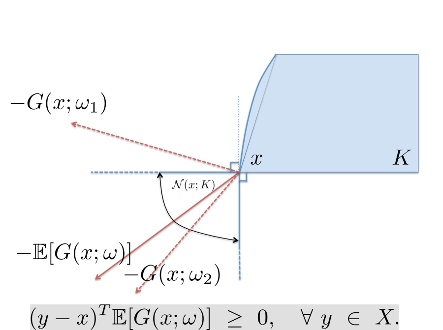
Figure 1: The stochastic variational inequality (SVI$(K,F)$): The expected-value formulation

Naturally, in instances where the expectation is simple to evaluate, as seen in Example  1 earlier, the resulting SVI$(K,F)$ is no harder than its deterministic counterpart. For instance, if the sample space $\Omega$ is finite, then the expectation reduces to a finite summation of deterministic maps which is itself a deterministic map. Consequently, the analysis of this problem is as challenging as a deterministic variational inequality problem. Unfortunately, in most stochastic regimes, this evaluation relies on a multi-dimensional integration and is not a straightforward task. In fact, a more general risk functional can be introduced instead of the expectation leading to a risk-based variational inequality problem that requires an $x$ such that

$$(\,y-x\,)^{T}\,\rho[G(x;\omega)]\,\geq\,0,\quad\forall\,y\,\in\,K,$$

where $\rho[G(x;\omega)]\triangleq\mathbb{E}[{G}(x;\omega)]+\mathbb{D}[G(x;\omega)]$ and $\mathbb{D}[\bullet]$ is a map incorporating dispersion measures such as standard deviation, upper semi-deviation, or the conditional value at risk (CVaR) (cf. [46, 47, 52] for recent advances in the optimization of these risk measures).

Extensions to set-valued and specializations to conic regimes follow naturally. For instance, if $K$ is a point-to-set mapping defined as $K:\mathbb{R}^{n}\to\mathbb{R}^{n}$, then the resulting problem is a stochastic quasi-variational inequality, and is denoted by SQVI$(K,F)$. When $K$ is a cone, then VI$(K,F)$ is equivalent to a complementarity problem CP$(K,F)$ and its stochastic generalization is given next.

Definition 1.2 (Stochastic complementarity problem (SCP$(K,F)$)).

Let $K$ be a closed and convex cone in $\mathbb{R}^{n}$, $G:\mathbb{R}^{n}\times\Omega\to\mathbb{R}^{n}$ be a single-valued mapping and $F(x)\triangleq\mathbb{E}[G(x;\omega)].$ Then the stochastic complementarity problem, denoted by SCP($K,F)$, requires an $x\in K$ such that

$$K\ \ni\ x\ \perp\ F(x)\ \in\ K^{*},\mbox{ where }F(x)=\mathbb{E}\left[G(x;\omega)\right].$$

∎

If the integrands of the expectation ($G(x;\omega)$) are multi-valued instead of single-valued, then we denote the mapping by $\Phi$. Accordingly, the associated variational problems are denoted by SVI$(K,\Phi)$, SQVI$(K,\Phi)$ and SCP$(K,\Phi)$.

The origin of the expected-value formulation can be traced to a paper by King and Rockafellar [26] where the authors considered a generalized equation [44, 45] with an expectation-valued mapping. Notably, the analysis and computation of the associated solutions are hindered significantly when the expectation is over a general measure space. Evaluating this integral is challenging, at best, and it is essential that specialized analytical and computational techniques be developed for this class of variational problems. From an analytical standpoint, Ravat and Shanbhag have developed existence statements for equilibria of stochastic Nash games that obviate the need to evaluate the expectation by combining Lebesgue convergence theorems with standard existence statements  [42, 43]. Our earlier worked focused on Nash games and examined such settings with nonsmooth payoff functions and stochastic constraints. It represents a starting point for our current study where we focus on more general variational inequality and complementarity problems and their generalizations and refinements. Accordingly, this paper is motivated by the need to provide sufficiency conditions for stochastic variational inequality problems, stochastic quasi-variational inequality problems, and stochastic complementarity problems. In addition, we consider variants when the variational maps are complicated by multi-valuednes. Stability statements for stochastic generalized equations have been provided by Liu, Römisch, and Xu [33].

From a computational standpoint, sampling approaches have addressed analogous stochastic optimization problems effectively [31, 51], but have focused relatively less on variational problems. In the latter context, there have been two distinct threads of research effort. Of these, the first employs sample-average approximation schemes [51]. In such an approach, the expectation is replaced by a sample-mean and the effort is on the asymptotic and rate analysis of the resulting estimators, which are obtainable by solving a deterministic variational inequality problem (cf. [13, 41, 54, 55]). A rather different track is adopted by Jiang and Xu [22] where a stochastic approximation scheme is developed for solving such stochastic variational inequality problems. Two regularized counterparts were presented by Koshal, Nedić, and Shanbhag [29, 28] where two distinct regularization schemes were overlaid on a standard stochastic approximation scheme (a Tikhonov regularization and a proximal-point scheme), both of which allow for almost-sure convergence. Importantly, this work also presents distributed schemes that can be implemented in networked regimes. A key shortcomings of standard stochastic approximation schemes is the relatively ad-hoc nature of the choice of steplength sequences. In [58], Yousefian, Nedić, and Shanbhag develop distributed stochastic approximation schemes where users can independently choose a steplength rule. Importantly, these rules collectively allow for minimizing a suitably defined error bound and are equipped with almost-sure convergence guarantees. Finally, Wang et al. [53] focus on developing a sample-average approximation method for expected-value formulations of the stochastic variational inequality problems while Lu and Budhiraja [34] examine the confidence statements associated with estimators associated with a sample-average approximation scheme for stochastic variational inequality problem, again with expectation-based maps.

1.1.2 The expected-residual minimization (ERM) formulation

While there are many problem settings where expected-value formulations are appropriate (such as when modeling risk-neutral decision-making in a competitive regime) but there are also instances where the expected-value formulation proves inappropriate. A case in point arises when attempting to obtain solutions to a variational inequality problem that are robust to parametric uncertainty; such problems might arise when faced with traffic equilibrium or structural design problems. Given a random mapping ${G}$, the almost-sure formulation of the stochastic variational inequality problem requires a (deterministic) vector $x\in K$ such that for almost every $\omega\in\Omega$,

$$(y-x)^{T}G(x;\omega)\,\geq\,0,\quad\forall\ y\,\in\,K.$$ (1)

Naturally, if $K$ is an $n-$dimensional cone, then (1) reduces to CP$(K,{G(.;\omega)})$, a problem that requires an $x$ such that for almost all $\omega\in\Omega$,

$$K\,\ni\,x\,\perp\,G(x;\omega)\,\in\,K^{*}.$$ (2)

Yet, we believe that obtaining such an $x$ is possible only in pathological settings. Instead, one approach for resolving such a problem has emerged through the minimization of the expected residual. For instance, if $K\triangleq\mathbb{R}^{n}_{+}$, this problem is a nonlinear complementarity problem (NCP) and for a fixed but arbitrary realization $\omega\in\Omega$, the residual of this system can be minimized as follows:

$${{\operatornamewithlimits{\mbox{minimize}}_{x\geq 0}}}\ \|\,\mathbf{\Phi}(x;\omega)\|,$$

where $\mathbf{\Phi}(x;\omega)$ denotes the equation reformulation of the NCP (See [10]). If the Fischer-Burmeister $\phi_{\rm FB}$ is chosen as the C-function, the expected residual minimization (ERM) problem in [6, 11] solves the following stochastic program to compute a solution of the stochastic NCP (2):

$$\begin{array}[]{ll}\displaystyle{{\operatornamewithlimits{\mbox{minimize}}_{x\geq 0}}}&\mathbb{E}\left[\left\|\,\Phi_{\rm FB}(x;\omega)\,\right\|\right],\\[7.0pt] \mbox{where}&\Phi_{\rm FB}(x;\omega)\,\triangleq\,\left(\,\sqrt{x_{i}^{2}+{G}_{i}(x;\omega)^{2}}-\left(\,x_{i}+{G}_{i}(x;\omega)\,\right)\,\right)_{i=1}^{n};\end{array}$$ (3)

see [32, equation (3.8)]. In [36], Luo and Lin minimize the expected residual while convergence analysis of the expected residual minimization (ERM) technique has been carried out in the context of stochastic Nash games [37] and stochastic variational inequality problems [35]. In more recent work, Chen, Wets, and Zhang [7] revisit this problem and present an alternate ERM formulation, with the intent of developing a smoothed sample average approximation scheme. In contrast with the expected-value formulation and the almost-sure formulation, Gwinner and Raciti [14, 15] consider an infinite-dimensional formulation of the variational inequality for capturing randomness and provide discretization-based approximation procedures for such problems.

The remainder of the paper is organized as follows. In section 2, we outline our assumptions used, motivate our study by considering two application instances, and provide the relevant background on integrating set-valued maps. In section 3, we recap our sufficiency conditions for the solvability of stochastic variational inequality problems with single and multi-valued mappings and we provide results for the stochastic quasi-variational inequality problems with single and multi-valued mappings. Refinements of the statements for SVIs are provided for the complementarity regime in Section 4 under varying assumptions on the map. Finally, in section 5, we revisit the motivating examples of section 2 and verify that the results developed in this paper are indeed applicable.

2 Assumptions, examples, and background

In Section 2.1, we provide a summary of the main assumptions employed in the paper. The utility of such models is demonstrated by discussing some motivating examples in Section 2.2. Finally, some background is provided on the integrals of set-valued maps in Section 2.3.

2.1 Assumptions

We now state the main assumptions used throughout the paper and refer to them when appropriate. The first of these pertains to the probability space.

Assumption 1 (Nonatomicity of measure $\mathbb{P}$).

The probability space ${\mathcal{P}}=(\Omega,{\mathcal{F}},\mathbb{P})$ is nonatomic.

The next assumption focuses on the properties of the single-valued map, referred to as $F$.

Assumption 2 (Continuity and integrability of $F$).

• ${\color[rgb]{0,0,0}G}:\mathbb{R}^{n}\times\Omega\to\mathbb{R}^{n}$ is a single-valued map. Furthermore, $G(x;\omega)$ is continuous in $x$ for almost every $\omega\in\Omega$ and is integrable in $\omega$, for every $x$.

• $F(x)=\mathbb{E}[G(x;\omega)]$ is continuous in $x$.

Note that, the assumption of Lipschitz continuity of $G(x;\omega)$ with an integrable Lipschitz constant implies that $\mathbb{E}[G(x;\omega)]$ is also Lipschitz continuous. We now recall the definition of integrably bounded set-valued maps to be used in the assumption to follow.

Definition 2.1 (Integrably bounded set-valued map).

A set-valued map $H$ that maps from $\Omega$ into nonempty, closed subsets of $\mathbb{R}^{n}$ is integrably bounded if there exists a nonnegative integrable function $k\in L^{1}(\Omega,\mathbb{R},\mathbb{P})$ such that

$$H(\omega)\subseteq k(\omega)B(0,1)\mbox{ almost everwhere}.$$

The next two assumptions pertain to the set-valued maps employed in this paper. When the map is multi-valued, to avoid confusion, we employ the notation $\Phi(x)$, defined as $\Phi(x)\triangleq\mathbb{E}[\Phi(x;\omega)]$, and impose the following assumptions.

Assumption 3 (Lower semicontinuity and integrability of $\Phi$).

$\Phi:\mathbb{R}^{n}\times\Omega\to 2^{\mathbb{R}^{n}}$ is a set-valued map satisfying the following:

• $\Phi(x;\omega)$ has nonempty and closed images for every $x$ and every $\omega\in\Omega$.

• $\Phi(x;\omega)$ is lower semicontinuous in $x$ for almost all $\omega\in\Omega$ and integrably bounded for every $x$.

Finally, when considering quasi-variational inequality problems, $K$ is a set-valued map, rather than a constant map.

Assumption 4.

The set-valued map $K:\mathbb{R}^{n}\to 2^{\mathbb{R}^{n}}$ is deterministic, closed-valued, convex-valued.

We conclude this subsection with some notation. $\textrm{cl}(U)$ denotes the closure of a set $U\subset\mathbb{R}^{n}$, $\textrm{bd}(U)$ denotes the boundary of the set $U$ and $\textrm{dom}(K)$ denotes the domain of the mapping $K$.

2.2 Examples

We now provide two instances of where stochastic variational problems arise in practice.

Nonsmooth stochastic Nash-Cournot equilibrium problems:

Cournot’s oligopolistic model is amongst the most widely used models for modeling strategic interactions between a set of noncooperative firms [12]. Under an assumption that firms produce a homogenous product, each firm attempts to maximize profits by making a quantity decision while taking as given, the quantity of its rivals. Under the Cournot assumption, the price of the good is assumed to be dependent on the aggregate output in the market. The resulting Nash equilibrium, qualified as the Nash-Cournot equilibrium, represents a set of quantity decisions at which no firm can increase profit through a unilateral change in quantity decisions. unilaterally changing the quantity of the product it produces. To accommodate uncertainty in costs and prices in Nash-Cournot models and loss of differentiability of price functions which can occur for example by introduction of price caps  [21] we consider a stochastic generalization of the classical deterministic Nash-Cournot model and allow for piecewise smooth price functions, as captured by the following assumption on costs and prices.

Assumption 5.

Suppose the cost function $c_{i}(x_{i})$ is an increasing convex twice continuously differentiable function for all $i=1,\ldots,N$. Let $X\triangleq\sum_{i=1}^{n}x_{i}$. Since $x_{i}$ denotes the quantity produced, $x_{i}\geq 0$. The price function $p(X;\omega)$ is a decreasing piecewise smooth convex function where $p(X;\omega)$ is given by

$$p(X;\omega)=\begin{cases}p^{1}(X;\omega),&0\leq X\leq\beta^{1}\\ p^{j}(X;\omega),&\beta^{j-1}\leq X\leq\beta^{j},j=2,\ldots,s\\ p^{s}(X;\omega),&\beta^{s}\leq X\end{cases}$$ (4)

where $p^{j}(X;\omega)=a^{j}(\omega)-b^{j}(\omega)X$ is a strictly decreasing affine function of $X$ for $j=1,\ldots,s$. Finally, $\beta^{1},\ldots,\beta^{s}$ are a set of increasing positive scalars and $(a^{j}(\omega),b^{j}(\omega))$ are positive in an almost-sure sense and integrable for $j=1,\ldots,s.$

Consider an $N-$player generalized Nash-Cournot game. Given the tuple of rival strategies $x_{-i}$, the $i$th player’s strategy set is given by $K_{i}(x_{-i})$ while his objective function is given by $\mathbb{E}[f_{i}(x;\omega)]\triangleq c_{i}(x_{i})-\mathbb{E}[p(x;\omega)x_{i}]$. Then $\{x_{i}^{*}\}_{i=1}^{N}$ denotes a stochastic Nash-Cournot equilibrium if $x_{i}^{*}$ solves the convex optimization problem G${}_{i}(x^{*}_{-i})$, defined as

$$\begin{array}[]{ll}\displaystyle{\operatornamewithlimits{\mbox{minimize}}_{x_{i}}}&\displaystyle\mathbb{E}[f_{i}(x;\omega)]\\ \mbox{subject to}&x_{i}\in K_{i}(x_{-i}).\end{array}$$

The equilibrium conditions of this problem are given a stochastic QVI with multi-valued mappings. In section 5, we revisit this problem with the intent of developing statements about existence of solutions

Strategic behavior in power markets:

Consider a power market model in which a collection of generation firms compete in a single-settlement market. Economic equilibria in power markets has been extensively studied using a complementarity framework; see [21, 20]. Our model below is based on the model of Hobbs and Pang [21] which we modify to account for uncertainty in prices and costs.

Consider a set of nodes ${\mathcal{N}}$ of a network. The set of generation firms is indexed by $f$, where $f$ belongs to the finite set ${\mathcal{F}}$. At a node $i$ in the network, a firm $f$ may generate $g_{fi}$ units at node $i$ and sell $s_{fi}$ units to node $i$. The total amount of power sold to node $i$ by all generating firms is $S_{i}$. The generator firms’ profits are revenue less costs. If the nodal power price at node $i$th is a random function given by $p_{i}(S_{i};\omega)$ where $p_{i}(S_{i};\omega)$ is a decreasing function of $S_{i}$, then the firms’ revenue is just the price times sales $s_{fi}$. The costs incurred by the firm $f$ at node $i$ are the costs of generating $g_{fi}$ and transmitting the excess $(s_{fi}-g_{fi})$. Let the cost of generation associated with firm $f$ at node $i$ be given by $c_{fi}(g_{fi};\omega)$ and the cost of transmitting power from an arbitrary node (referred to as the hub) to node $i$ be given by $w_{i}$. The constraint set ensures a balance between sales and generation at all nodes, nonnegative sales and generation and generation subject to a capacity limit. The price and cost functions are assumed to satisfy the following requirement.

Assumption 6.

For $i\in{\mathcal{N}}$, the price function $p_{i}(S_{i};\omega)$ is a decreasing function with its absolute value bounded above by a nonnegative integrable function $\bar{p}_{i}(\omega)$. Furthermore, the cost functions $c_{fi}(g_{fi};\omega)$ are nonnegative and increasing.

The resulting problem faced by generating firm $f$ requires determining sales $s_{fi}$ and generation $g_{fi}$ at all nodes $i$ and is captured as follows:

$$\begin{array}[]{ll}\displaystyle{{\operatornamewithlimits{\mbox{maximize}}_{s_{fi},\,g_{fi}}}}&\mathbb{E}\left[\displaystyle{\sum_{i\in{\mathcal{N}}}}\,\left(\,p_{i}(S_{i};\omega)s_{fi}-c_{fi}(g_{fi};\omega)-(s_{fi}-g_{fi})w_{i}\,\right)\right]\\[14.45377pt] \mbox{subject to}&\left\{\begin{array}[]{lll}0&\leq&g_{fi}\,\leq\,{\rm cap}_{fi}\\[5.0pt] 0&\leq&s_{fi}\end{array}\right\},\quad\forall\,i\in{\mathcal{N}}\\[28.90755pt] \mbox{and}&\displaystyle{\sum_{i\in{\mathcal{N}}}}\,(\,s_{fi}-g_{fi}\,)\,=\,0.\end{array}$$

Note that, the generating firm sees the transmission fee $w_{i}$ and the rival firms’ sales $s_{-fi}\equiv\{s_{hi}~{}:~{}h\neq f\}$ as exogenous parameters to its optimization problem even though they are endogenous to the overall equilibrium model as we will see shortly. The ISO sees the transmission fees $w=(w_{i})_{i\in{\mathcal{N}}}$ as exogenous and prescribes flows $y=(y_{i})_{i\in{\mathcal{N}}}$ as per the following linear program

$$\begin{array}[]{ll}\displaystyle{{\operatornamewithlimits{\mbox{maximize}}}}&\displaystyle{\sum_{i\in{\mathcal{N}}}}\,y_{i}w_{i}\\[14.45377pt] \mbox{subject to}&\displaystyle{\sum_{i\in{\mathcal{N}}}}\,{\rm PDF}_{ij}y_{i}\,\leq\,T_{j},\qquad\forall\,j\in{\mathcal{K}},\end{array}$$

where ${\mathcal{K}}$ is the set of all arcs or links in the network with node set ${\mathcal{N}}$, $T_{j}$ denotes the transmission capacity of link $j$, $y_{i}$ represents the transfer of power (in MW) by the system operator from a hub node to node node $i$ and PDF_ij denotes the power transfer distribution factor, which specifies the MW flow through link $j$ as a consequence of unit MW injection at an arbitrary hub node and a unit withdrawal at node $i$.

Finally, to clear the market, the transmission flows $y_{i}$ must must balance the net sales at each node:

$$y_{i}\,=\,\displaystyle{\sum_{f\in{\mathcal{F}}}}\,\left(\,s_{fi}-g_{fi}\,\right),\qquad\forall\,i\in{\mathcal{N}}.$$

The above market equilibrium problem which comprises of each firm’s problem, the ISO’s problem and market-clearing condition, can be expressed as a stochastic complementarity problem by following the technique from [21]. This equivalent formulation of the above market equilibrium problem is described in the last section 5. We also illustrate the solvability of such problems using the framework developed in this paper.

2.3 Background on integrals of set-valued mappings

Recall that by Assumption 1, $(\Omega,{\mathcal{F}},\mathbb{P})$ is a nonatomic continuous probability space. Consider a set-valued map $H$ that maps from $\Omega$ into nonempty, closed subsets of $\mathbb{R}^{n}$ . We recall three definitions from [1, Ch. 8]

Definition 2.2 (Measurable set-valued map).

A map $H$ is measurable if the inverse image of each open set in $\mathbb{R}^{n}$ is a measurable set: for all open sets $O\subseteq\mathbb{R}^{n}$, we have

$$H^{-1}(O)=\left\{\omega\in\Omega\mid H(\omega)\cap O\neq\emptyset\right\}\in{\mathcal{F}}.$$

Definition 2.3 (Measurable selection).

Suppose a measurable map $h:\Omega\to\mathbb{R}^{n}$ satisfies $h(\omega)\in H(\omega)$ for almost all $\omega\in\Omega$. Then $h$ is called a measurable selection of $H$.

The existence of a measurable selection is proved in [1, Th. 8.1.3].

Definition 2.4 (Integrable selection).

A measurable selection $h:\Omega\to\mathbb{R}^{n}$ is an integrable selection if $\mathbb{E}[h(\omega)]<\infty$ where

$$\mathbb{E}[h(\omega)]=\int_{\Omega}hd\mathbb{P}<\infty.$$

The set of all integrable selections of $H$ is denoted by ${\cal H}$ and is defined as follows:

$${\cal H} \triangleq\left\{h\in L^{1}(\Omega,{\mathcal{F}},\mathbb{P}):h(\omega)\in H(\omega)\hbox{ for almost all }\omega\in\Omega\right\},$$

Definition 2.5 (Expectation of a set-valued map).

The expectation of the set-valued map $H$, denoted by $\mathbb{E}[H(\omega)]$, is the set of integrals of integrable selections of $H$:

$$\mathbb{E}[H(\omega)]\triangleq\int_{\Omega}Hd\mathbb{P}\triangleq\left\{\int_{\Omega}hd\mathbb{P}\mid h\in{\cal H}\right\}.$$

If the images of $H(\omega)$ are convex then this set-valued integral is convex [1, Definition 8.6.1]. If the assumption of convexity of images of $H$ does not hold, then the convexity of this integral follows from Th. 8.6.3 [1], provided that the probability measure is nonatomic. We make precisely such an assumption (See Assumption 1) and are therefore guaranteed that the integral of the set-valued map $H$ is a convex set [1, Th. 8.6.3].

Recall that a point $\bar{z}$ of a convex set $K$ is said to be extremal if there are no two points $x,y\in K$ such that $\lambda x+(1-\lambda)y=\bar{z}$ for $\lambda\in(0,1)$ and is denoted by ${\bar{z\mkern 2.8mu}\mkern-2.8mu}{}\in\textrm{ext}(K).$ Similarly, as per Def. 8.6.5 [1], we define an extremal selection as follows:

Definition 2.6 (Extremal selection).

Given the convex set $\int_{\Omega}Hd\mathbb{P}$, an integrable selection $h\in{\cal H}$ is an extremal selection of $H$ if

$$\int_{\Omega}hd\mathbb{P}\hbox{ is an extremal point of the closure of the convex set }\int_{\Omega}Hd\mathbb{P}.$$

The set of all extremal selections is denoted by ${\cal H}_{e}$ and is defined as follows:

$${\cal H}_{e}\triangleq\left\{h\in{\cal H}\mid\int_{\Omega}hd\mathbb{P}\in\textrm{ext}\left(\textrm{cl}\left(\int_{\Omega}Hd\mathbb{P}\right)\right)\right\}.$$

By Theorem  [1, Th. 8.6.3], we have the following Lemma for the representation of extremal points of closure of $\int_{\Omega}Hd\mathbb{P}$.

Theorem 1 (Representation of extreme points of set-valued integral [1, Th. 8.6.3]).

Suppose Assumption 1 holds and let $H$ be a measurable set-valued map from $\Omega$ to subsets of $\mathbb{R}^{n}$ with nonempty closed images. Then the following hold:

• $\int_{\Omega}Hd\mathbb{P}$ is convex and extremal points of ${\textrm{cl}}(\int_{\Omega}Hd\mathbb{P})$ are contained in $\int_{\Omega}Hd\mathbb{P}$.

• If $x\in{\textrm{ext}}\left({\textrm{cl}}\left(\int_{\Omega}Hd\mathbb{P}\right)\right)$, then there exists a unique $h\in{\cal H}_{e}$ with $x=\int_{\Omega}hd\mathbb{P}$.

• If $H$ is integrably bounded, then the integral $\int_{\Omega}Hd\mathbb{P}$ is also compact.

As a corollary to the above theorem, we have a representation of points in a set-valued integral as follows.

Corollary 2 (Representation of points in a set-valued integral [1, Th. 8.6.6]).

Let $H$ be a measurable integrably bounded set-valued map from $\Omega$ to subsets of $\mathbb{R}^{n}$ with nonempty closed images. If $\mathbb{P}$ is nonatomic, then for every $x\in\int_{\Omega}Hd\mathbb{P}$, there exist $n+1$ extremal selections $h_{k}\in{\cal H}_{e}$ and $n+1$ measurable sets $A_{k}\in{\mathcal{F}}$, $k=0,\cdots,n$, such that

$$x=\displaystyle\int_{\Omega}\left(\sum_{k=1}^{n}\chi_{\tiny A_{k}}h_{k}\right)d\mathbb{P}$$

where $\chi_{A_{k}}$ is the characteristic function of $A_{k}$.

3 Stochastic quasi-variational inequality problems

In this section, we develop sufficiency conditions for the solvability of stochastic quasi-variational inequality problems under a diversity of assumptions on the map. More specifically, we begin by recapping sufficiency conditions for the solvability of stochastic variational inequality problems with single-valued and multi-valued maps in Section 3.1. In many settings, the variational inequality problems may prove incapable of capturing the problem in question. For instance, the equilibrium conditions of convex generalized Nash games are given by a quasi-variational inequality problem. As mentioned earlier, when the constant map $K$ is replaced by a set-valued map $K:\mathbb{R}^{n}\to\mathbb{R}^{n}$, the resulting problem is an SQVI. In this section, we extend the sufficiency conditions presented in the earlier section to accommodate the SQVI$(K,F)$ (Section 3.2) and SQVI$(K,\Phi)$ (Section 3.3), respectively. Throughout this section, Assumption 4 holds for the set-valued map $K$.

3.1 SVIs with single-valued and multi-valued mappings

In this section, we begin by assuming that the scenario-based mappings $G(\bullet;\omega)$ are single-valued for each $\omega\in\Omega$. With this assumption, we provide sufficient conditions that the scenario-based VI$(K,G(\bullet;\omega))$ must satisfy in order to conclude the existence of solution to the stochastic SVI($K,F$) without requiring the evaluation of expectation operator. Recall that in SVI($K,F$), $F(x)=\mathbb{E}[G(x;\omega)]$. In particular, in the next proposition, we show that if a certain coercivity condition holds for the scenario-based map $G(\bullet;\omega)$ in an almost-sure sense then existence of the solution to the above SVI may be concluded without resorting to formal evaluation of the expectation.

Proposition 3 (Solvability of SVI($K,F$)).

Consider a stochastic variational inequality SVI$(K,F)$. Suppose Assumption 2 holds. Suppose there exists an $x^{\textrm{ref}}\in K$ such that the following hold:

• $\displaystyle\liminf_{\|x\|\to\infty,x\in K}\left[G(x;\omega)^{T}(x-x^{\textrm{ref}})\right]>0\text{ almost surely;}$

• Suppose there exists a nonnegative integrable function $u(\omega)$ such that ${G(x;\omega)^{T}(x-x^{\textrm{ref}})}\geq-u(\omega)$ holds almost surely for any $x$.

Then the stochastic variational inequality SVI$(K,F)$ has a solution.

Proof.

See appendix.∎

In settings where $K$ is a Cartesian product, defined as

$$K\triangleq\prod_{\nu=1}^{N}K_{\nu},$$ (5)

VI$(K,F)$ is a partitioned variational inequality probem, as defined in  [10, Ch. 3.5]. Accordingly, Proposition 3 can be weakened so that even if the coercivity property holds for just one index $\nu\in\{1,\ldots,N\}$, the stochastic variational inequality is solvable.

Proposition 4 (Solvability of SVI($K,F$) for Cartesian $K$).

Consider a stochastic variational inequality SVI$(K,F)$ where $K$ is a Cartesian product of closed and convex sets as specified in (5). Suppose that Assumption 2 and the following hold:

• There exists an $x^{\textrm{ref}}\in K$ and an index $\nu\in\{1,\ldots,N\}$ such that for any $x\in K$,

  $$\liminf_{\|x_{\nu}\|\to\infty,x_{\nu}\in K_{\nu}}\left[{G}_{\nu}(x;\omega)^{T}(x_{\nu}-x^{\textrm{ref}}_{\nu})\right]>0$$

  holds in an almost sure sense; and

• For the above $\nu$ and for any $x$, suppose there exists a nonnegative integrable function $u(\omega)$ such that ${G_{\nu}(x;\omega)^{T}(x_{\nu}-x^{\textrm{ref}}_{\nu})}\geq-u(\omega)$ holds almost surely for any $x$.

Then SVI$(K,F)$ admits a solution.

Proof.

See appendix. ∎

It is well known that strong monotonicity of the map $F$ and convexity of the set $K$ guarantee existence of solution for the deterministic VI$(K,F)$ [10, Theorem 2.3.3]. In fact, it may be recalled that if $F(x)$ is a strongly monotone map then for any reference vector $x^{\rm ref}\in K$, we have that

$$\quad\liminf_{x\in K,\|x\|\to\infty}{F(x)^{T}(x-x^{\rm ref})}=\liminf_{x\in K,\|x\|\to\infty}{(F(x)-F(x^{\rm ref})+F(x^{\rm ref}))^{T}(x-x^{\rm ref})}$$

$$\geq\liminf_{x\in K,\|x\|\to\infty}\left[\eta\|x-x^{\rm ref}\|^{2}+{F(x^{\rm ref})^{T}(x-x^{\rm ref})}\right]=+\infty,$$

where the first term tends to $+\infty$ at a quadratic rate while the second term may tend to $\pm\infty$ at a linear rate. In effect, we have that when $F(x)$ is a strongly monotone map, the coercivity requirement holds immediately and existence follows. It follows that if ${G}(x;\omega)$ is a strongly monotone map for almost every $\omega$ with constant $\eta(\omega)$ where $\eta(\omega)\geq\eta$ a.s., then $F(x)$ is a strongly monotone map and SVI$(K,F)$ is solvable with a unique solution. We now present a similar result for stochastic variational inequalities SVI$(K,F)$ under the assumption that the mapping $G(x;\omega)$ is a monotone mapping over $K$ for almost every $\omega\in\Omega$, a weaker set of sufficient conditions as compared to Propositon 3 guarantees existence of solution for SVI($K,F$).

Corollary 5 (Solvability of SVI($K,F$) under monotonicity).

Consider SVI$(K,F)$ and suppose that Assumption 2 holds. Further, let $G(x;\omega)$ be a monotone mapping on $K$ for almost every $\omega\in\Omega.$ Suppose there exists an $x^{\textrm{ref}}\in K$ such that the following hold:

• $\displaystyle\liminf_{\|x\|\to\infty,x\in K}\left[G(x^{\textrm{ref}};\omega)^{T}(x-x^{\textrm{ref}})\right]>0$ holds in almost sure sense;

• Suppose there exists a nonnegative integrable function $u(\omega)$ such that ${G(x^{\textrm{ref}};\omega)^{T}(x-x^{\textrm{ref}})}\geq-u(\omega)$ holds almost surely for any $x$.

Then SVI$(K,F)$ is solvable.

Proof.

See appendix.∎

Next, we consider a stochastic variational inequality SVI$(K,\Phi)$ where $\Phi(x)\triangleq\mathbb{E}[\Phi(x;\omega)]$ and $\Phi(x;\omega)$ is a multi-valued mapping. Before proceeding to prove existence of solutions to SVIs with multi-valued maps, we restate Corollary 2 for the case of the set-valued integral $\Phi(x)=\mathbb{E}[\Phi(x;\omega)]$ of interest.

Lemma 6 (Representation of elements of set-valued integral as an integral of convex combination of extremal selections).

Suppose Assumption 1 holds. Let $\Phi$ be a measurable integrably bounded set-valued map from $\mathbb{R}^{n}\times\Omega$ to subsets of $\mathbb{R}^{n}$ with closed nonempty images. Then any $w\in\mathbb{E}[\Phi(x;\omega)]$ can be expressed as

$$w=\displaystyle\int_{\Omega}g(x;\omega)d\mathbb{P}$$

where $g(x;\omega)=\sum_{k=1}^{n}\lambda_{k}(x)f_{k}(x;\omega)$ and $\lambda_{k}(x)\geq 0,\sum_{k=0}^{n}\lambda_{k}(x)=1$ and each $f_{k}(x;\omega)$ is an extremal selection of $\Phi(x;\omega)$.

Proof.

Since $w\in\mathbb{E}[\Phi(x;\omega)]$ and $\mathbb{E}[\Phi(x;\omega)]$ is a convex set, thus by Carath$\acute{\textrm{e}}$odory’s theorem for convex sets, there exists $\lambda_{k}(x)\geq 0,w_{k}\in{\textrm{ext}}\left({\textrm{cl}}\left(\mathbb{E}[\Phi(x;\omega)]\right)\right)$ such that

$$w=\sum_{k=0}^{n}\lambda_{k}(x)w_{k},\quad\sum_{k=0}^{n}\lambda_{k}(x)=1$$

Now, since $w_{k}\in{\textrm{ext}}\left({\textrm{cl}}\left(\mathbb{E}[\Phi(x;\omega)]\right)\right)$, by [1, Th. 8.6.3], for each index $k$, there exists an extremal selection $f_{k}(x;\omega)$ from $\Phi(x;\omega)$ such that $\int_{\Omega}f_{k}(x;\omega)d\mathbb{P}=w_{k}$. Thus, we obtain

$$w=\sum_{k=0}^{n}\lambda_{k}(x)\int_{\Omega}f_{k}(x;\omega)d\mathbb{P},$$

which can be rewritten as

$$w=\displaystyle\int_{\Omega}g(x;\omega)d\mathbb{P}$$

where $g(x;\omega)=\sum_{k=0}^{n}\lambda_{k}(x)f_{k}(x;\omega)$. The required representation result follows. ∎

We begin by providing a coercivity-based sufficiency condition for deterministic multi-valued variational inequalities [25].

Theorem 7 (Solvability of VI $(K,\Phi)$[25, Th. 2.1,2.2]).

Suppose $K$ is a closed and convex set in $\mathbb{R}^{n}$ and let $\Phi:K\rightrightarrows\mathbb{R}^{n}$ be a lower semicontinuous multifunction with nonempty closed and convex images. Consider the following statements:

1. Suppose there exists an $x^{\textrm{ref}}\in K$ such that $L_{<}(K,\Phi)$ is bounded (possibly empty) where

   $$L_{<}(K,\Phi)\triangleq\left\{x\in K:\inf_{y\in\Phi(x)}(x-x^{\textrm{ref}})^{T}y<0\right\}.$$ (6)

2. The variational inequality VI$(K,\Phi)$ is solvable

Then, (a) implies (b). Furthermore, if $\Phi(x)$ is a pseudomonotone mapping over $K$, then (a) is equivalent to (b).

Using this condition, we proceed to develop sufficiency conditions for the existence of solutions to SVI$(K,\Phi).$

Proposition 8 (Solvability of SVI$(K,\Phi)$).

Consider SVI$(K,\Phi)$ and suppose assumptions 1 and 3 hold. Further, suppose the following hold:

1. Suppose there exists an $x^{\textrm{ref}}\in K$ such that

   $$\liminf_{x\in K,\|x\|\to\infty}\left({\inf_{w\in\Phi(x;\omega)}w^{T}(x-x^{\textrm{ref}})}\right)>0\mbox{ almost surely}.$$

2. For the above $x^{\textrm{ref}}$, suppose there exists a nonnegative integrable function $u(\omega)$ such that $g(x;\omega)^{T}(x-x^{\textrm{ref}})\geq-u(\omega)$ holds almost surely for any integrable selection $g(x;\omega)$ of $\Phi(x;\omega)$ and for any $x$.

Then SVI$(K,\Phi)$ is solvable.

Proof.

The proof proceeds in two parts.

• We first show that the following coercivity condition holds for the expected value map: there exists an $x^{\textrm{ref}}\in K$ such that

  $$\liminf_{x\in K,\|x\|\to\infty}\left({\inf_{w\in\Phi(x)}w^{T}(x-x^{\textrm{ref}})}\right)>0.$$ (7)

• If (a) holds, then we show that for the given $x^{\textrm{ref}}\in K$, the set $L_{<}(K,\Phi)$ is bounded (possibly empty) where $L_{<}(K,\Phi)$ is defined in (6).

Proof of (a):

We proceed by a contradiction and assume that (7) does not hold for the expected value map. Thus, for any $x^{\textrm{ref}}$, there exists a sequence $x_{k}\in K$ with $\|x_{k}\|\to\infty$ such that

$$\liminf_{k\to\infty}\left({\inf_{w\in\Phi(x_{k})}w^{T}(x_{k}-x^{\textrm{ref}})}\right)\leq 0.$$

Since $\Phi(x_{k})$ is a closed set, the infimum above is attained at $y_{k}\in\Phi(x_{k})$. Thus, we have

$$\liminf_{k\to\infty}\left[y_{k}^{T}(x_{k}-x^{\textrm{ref}})\right]\leq 0$$ (8)

Now, $y_{k}\in\Phi(x_{k})=\mathbb{E}[\Phi(x_{k};\omega)]$. By the representation Lemma (Lemma  6), since $y_{k}\in\Phi(x_{k})$, we have that

$$y_{k}=\displaystyle\int_{\Omega}g_{k}(x_{k};\omega)d\mathbb{P}$$

for some $g_{k}(x_{k};\omega)=\sum_{l=1}^{n}\lambda_{l}(x_{k})f_{l}(x_{k};\omega)$ where $\lambda_{l}(x_{k})\geq 0,\sum_{l=0}^{n}\lambda_{l}(x)=1$ and each $f_{l}(x_{k};\omega)$ is an extremal selection of $\Phi(x_{k};\omega)$. With this substitution, (8) becomes

$$\liminf_{k\to\infty}\left[\displaystyle\int_{\Omega}g_{k}(x_{k};\omega)^{T}(x_{k}-x^{\textrm{ref}})d\mathbb{P}\right]\leq 0.$$

By hypothesis (ii), we may use Fatou’s Lemma to interchange the order of integration and limit infimum, as shown next:

$$\displaystyle\int_{\Omega}\liminf_{k\to\infty}\left[~{}g_{k}(x_{k};\omega)^{T}(x_{k}-x^{\textrm{ref}})\right]d\mathbb{P}\leq 0.$$

Consequently, there is a set of positive measure $U\subseteq\Omega$, over which the integrand is nonpositive or

$$\liminf_{k\to\infty}~{}\left[g_{k}(x_{k};\omega)^{T}(x_{k}-x^{\textrm{ref}})\right]\leq 0,\quad\forall\omega\in U.$$

Substituting the expression for $g_{k}$, we obtain the following inequality.

$$\liminf_{k\to\infty}~{}\left[(x_{k}-x^{\textrm{ref}})^{T}\left(\sum_{l=1}^{n}\lambda_{l}(x_{k})f_{l}(x_{k};\omega)\right)\right]\leq 0,\quad\forall\omega\in U.$$

As a result, for at least one index $l\in\{1,...,n\}$, we have that

$$\liminf_{k\to\infty}~{}\left[\lambda_{l}(x_{k})f_{l}(x_{k};\omega)^{T}(x_{k}-x^{\textrm{ref}})\right]\leq 0,\quad\forall\omega\in U.$$

Since $0\leq\lambda_{l}(x_{k})\leq 1$, the following must be true for the above $l$:

$$\liminf_{k\to\infty}\left[f_{l}(x_{k};\omega)^{T}(x_{k}-x^{\textrm{ref}})\right]\leq 0,\quad\forall\omega\in U.$$

Moreover, $f_{l}(x_{k};\omega)\in\Phi(x_{k};\omega)$ since it is an extremal selection and we have that

$$\liminf_{k\to\infty}\left[\inf_{w\in\Phi(x_{k};\omega)}w^{T}(x_{k}-x^{\textrm{ref}})\right]\leq 0,\quad\forall\omega\in U.$$

Since, this holds for any $x^{\textrm{ref}}$, it holds for the vector $x^{\textrm{ref}}$ in the hypothesis and for a set of positive measure $U$, we have that

$$\liminf_{x\in K,\|x\|\to\infty}\left[{\inf_{w\in\Phi(x;\omega)}w^{T}(x-x^{\textrm{ref}})}\right]\leq 0,\forall\omega\in U.$$

This contradicts the hypothesis and condition (7) must hold for the expected value map.

Proof of (b)

Next, we show that when the condition (7) holds for the expected value map, for the given $x^{\textrm{ref}}\in K$, the set $L_{<}(K,\Phi)$ is bounded (possibly empty) where $L_{<}(K,\Phi)$ is defined in (6). We proceed by contradiction and assume that $L_{<}(K,\Phi)$ is nonempty and unbounded. Then, there exists a sequence $\{x_{k}\}\in L_{<}(K,\Phi)$ with $\|x_{k}\|\to\infty$. Since $x_{k}\in L_{<}(K,\Phi)$, we have for each $k$,

$$\inf_{y\in\Phi(x_{k})}\left[(x_{k}-x^{\textrm{ref}})^{T}y\right]<0.$$

This implies that for the sequence $\{x_{k}\}$, we have that

$$\liminf_{x_{k}\in K,\|x_{k}\|\to\infty}\left[{\inf_{w\in\Phi(x_{k})}w^{T}(x_{k}-x^{\textrm{ref}})}\right]\leq 0.$$

But this contradicts the coercivity property of the expected value map proved earlier:

$$\liminf_{x\in K,\|x\|\to\infty}\left[{\inf_{w\in\Phi(x)}w^{T}(x-x^{\textrm{ref}})}\right]>0.$$

This contradiction implies that $L_{<}(K,\Phi)$ is bounded and by Theorem 7, SVI$(K,\Phi)$ is solvable. ∎

3.2 SQVIs with single-valued mappings

Our first result is an extension of [10, Cor. 2.8.4] to the stochastic regime. In particular, we assume that the mapping $\mathbb{E}\left[G(x;\omega)\right]$ cannot be directly obtained; instead, we provide an existence statement that relies on the scenario-based map $G(x;\omega)$.

Proposition 9 (Solvability of SQVI($K,F$)).

Suppose Assumptions 2 and 4 hold. Furthermore, suppose there exists a bounded open set $U\subset\mathbb{R}^{n}$ and a vector $x^{\textrm{ref}}\in U$ such that the following hold:

1. For every $\bar{x}\in\textrm{cl}(U)$, the image $K(\bar{x})$ is nonempty and $\displaystyle\lim_{x\to\bar{x}}K(x)=K(\bar{x});$

2. $x^{\textrm{ref}}\in K(x)$ for every $x\in\textrm{cl}(U);$

3. $L_{<}(K,G;{\omega})\cap\textrm{bd}(U)=\emptyset$ holds almost surely, where

   $$L_{<}(K,G;{\omega})\triangleq\displaystyle\left\{x\in K(x)~{}|~{}(x-x^{\textrm{ref}})^{T}G(x;\omega)<0\displaystyle\right\}.$$ (9)

Then, SQVI($K,F$) has a solution where $F(x)=\mathbb{E}\left[G(x;\omega)\right].$

Proof.

Recall that by [10, Cor. 2.8.4], the stochastic SQVI($K,F$) is solvable if $L_{<}(K,F)\cap\textrm{bd}(U)=\emptyset,$ where

$$L_{<}(K,F)\triangleq\displaystyle\left\{x\in K(x)~{}|~{}(x-x^{\textrm{ref}})^{T}\mathbb{E}\left[G(x;\omega)\right]<0\displaystyle\right\}.$$

We proceed by contradiction and assume that there exists an $x\in L_{<}(K,F)$ and $x\in\textrm{bd}(U)$. By assumption, since $L_{<}(K,G;\omega)\cap\mbox{bd}(U)=\emptyset$ and $x\in\mbox{bd}(U)$, it follows that $x\notin L_{<}(K,G;{\omega})$ almost surely. This implies that $(x-x^{\textrm{ref}})^{T}G(x;\omega)\geq 0$ for all $\omega\in\Omega$. It follows that $(x-x^{\textrm{ref}})^{T}\mathbb{E}[G(x;\omega)]\geq 0,$ implying that $x\notin L_{<}(K,F)$. This contradicts our assertion that $x\in L_{<}(K,F)$. Therefore, we must have that $L_{<}(K,F)\cap\textrm{bd}(U)=\emptyset$ and by [10, Cor. 2.8.4], the stochastic SQVI($K,F$) has a solution. ∎

Another avenue for ascertaining existence of equilibrium in stochastic regimes is an extension of Harker’s result [17, Th. 2] which we present next.

Theorem 10 (Solvability of SQVI($K,F$) under compactness).

Suppose Assumptions 2 and 4 hold and there exists a nonempty compact convex set $\Gamma$ such that the following hold:

• $K(x)\subseteq\Gamma$, $\forall x\in\Gamma$;

• $K$ is a nonempty, continuous, closed and convex-valued mapping on $\Gamma$.

Then the SQVI($K,F$) has a solution.

Proof.

Since $F$ is continuous by Assumption 2(ii), all conditions of [17, Th. 2] hold. Thus, the SQVI($K,F$) has a solution. ∎

The above theorem relies on properties of the map $K$ and the continuity of the map $F$ to ascertain existence of solution. By Assumption 2, continuity of the map $F$ holds in the settings we consider and thus the solvability of SQVI($K,F$) follows readily. This theorem has a slightly different flavor compared to other results in this paper in the sense that we do not look at properties of the scenario-based map (other than continuity) that then guarantee existence of solution. We have listed this theorem here for completeness as it presents an alternate perspective of looking at the question of solvability of SQVI($K,F$).

3.3 SQVIs with multi-valued mappings

In this section, we relax the assumption of single-valuedness of the scenario-based mappings $G(\bullet;\omega)$ and instead allow for the map $\Phi(\bullet;\omega)$ to be multi-valued. In the spirit of the rest of this paper, our interest lies in deriving results that do not rely on evaluation of expectation. We use the concepts of set-valued integrals discussed in the previous section 2.3 and require that Assumption 4 holds throughout this subsection. Our first existence result relies on a sufficiency condition for generalized quasi-variational inequalities [5, Cor. 3.1]. We recall  [5, Cor. 3.1] which can be applied to the multi-valued SQVI($K,\Phi$).

Proposition 11 ([5, Cor. 3.1]).

Consider the SQVI($K,\Phi$). Suppose that there exists a nonempty compact convex set $C$ such that the following hold:

1. $K(C)\subseteq C$;

2. $\mathbb{E}[\Phi(x;\omega)]$ is a nonempty contractible-valued and compact-valued upper semicontinuous mapping on $C$;

3. $K$ is nonempty continuous convex-valued mapping on $C$.

Then the stochastic SQVI($K,\Phi$) admits a solution

However, this result requires evaluating $\mathbb{E}[\Phi(x;\omega)]$, an object that admits far less tractability; instead, we develop almost-sure sufficiency conditions that imply the requirements of Proposition 11.

Proposition 12 (Solvability of SQVI($K,\Phi)$)).

Suppose Assumptions 3 ans 4 hold. Furthermore, suppose there exists a nonempty compact convex set $C$ such that the following hold:

1. $K(C)\subseteq C$;

2. $\Phi(x;\omega)$ is a nonempty upper semicontinuous mapping for $x\in C$ in an almost-sure sense;

3. $K$ is nonempty, continuous and convex-valued mapping on $C$.

Then the stochastic SQVI($K,\Phi$) admits a solution.

Proof.

From Proposition 11, it suffices to show that under the above assumptions, $\mathbb{E}[\Phi(x;\omega)]$ is a nonempty contractible-valued, compact-valued, upper semicontinuous mapping on $C$.

1. $\mathbb{E}[\Phi(x;\omega)]$ is nonempty: Since $\Phi(x;\omega)$ is lower semicontinuous, it is a measurable set-valued map. Since it is a measurable set-valued map with nonempty closed images, by Aumann’s measurable selection theorem [1, Th. 8.1.3], there exists a measurable selection $h$ from $\Phi(x;\omega)$. Since $\Phi(x;\omega)$ is integrably bounded, every measurable selection is integrable. Thus, $\int_{\Omega}hd\mathbb{P}\in\int_{\Omega}\Phi(x;\omega)$, implying that $\mathbb{E}[\Phi(x;\omega)]$ is nonempty.

2. $\mathbb{E}[\Phi(x;\omega)]$ is contractible-valued: Since the probability space is nonatomic by definition, we have that $\mathbb{E}[\Phi(x;\omega)]$ is a convex set. Since a convex set is contractible, we have that $\mathbb{E}[\Phi(x;\omega)]$ is contractible.

3. $\mathbb{E}[\Phi(x;\omega)]$ is compact-valued: Since $\Phi(x;\omega)$ is integrably bounded, by [1, Th. 8.6.3], we get that $\mathbb{E}[\Phi(x;\omega)]$ is compact.

4. $\mathbb{E}[\Phi(x;\omega)]$ is upper semicontinuous: By hypothesis, we have that $\Phi(x;\omega)$ is a measurable, integrably bounded and upper-semicontinuous $x\in C$. Thus, from  [2, Cor. 5.2], it follows that $\mathbb{E}[\Phi(x;\omega)]$ is upper semicontinuous.

∎

The previous result relies on the compact-valuedness of $K$ with respect to a compact set $C$, a property that cannot be universally guaranteed. An alternate result for deterministic generalized QVI problems [5, Cor. 4.1] leverages coercivity properties of the map $\Phi(x)$ to claim existence of a solution. We state this result next.

Proposition 13 ([5, Cor. 4.1]).

Let $K$ be a set-valued map from $\mathbb{R}^{n}$ to subsets of $\mathbb{R}^{n}$ and $\Phi$ from $\mathbb{R}^{n}$ to subsets of $\mathbb{R}^{n}$ be a measurable integrably bounded set-valued map with closed nonempty images. Suppose that there exists a vector $x^{\textrm{ref}}$ such that

$$x^{\textrm{ref}}\in\underset{x\in\textrm{dom}(K)}{\bigcap}K(x)$$

$$\mbox{ and }\lim_{\|x\|\to\infty,x\in K(x)}\left[\inf_{y\in\Phi(x)}{(x-x^{\textrm{ref}})^{T}y\over{\|x\|}}\right]=\infty.$$ (10)

Suppose the following hold:

• $\Phi(x)$ is a nonempty, contractible-valued, compact-valued, upper semicontinuous map on $\mathbb{R}^{n}$;

• $K$ is convex-valued;

• There exists a $\rho_{0}>0$ such that $K(x)\cap B_{\rho}$ is a continuous mapping for all $\rho>\rho_{0}$ where $B_{\rho}$ is a ball of radius $\rho$ centered at the origin.

Then for each vector $q$, SQVI($K,\Phi+q$) has a solution. Moreover, there exists an $r>0$ such that $\|x^{*}\|<r$ for each solution $(x^{*},y^{*})$.

In the next proposition, by using the properties of $\Phi(x;\omega)$, we develop an integration-free analog of this result for multi-valued SQVI$(K,\Phi)$.

Proposition 14 (Solvability of SQVI($K,\Phi$)).

Suppose Assumptions 3 and 4 hold. Suppose that there exists a vector $x^{\textrm{ref}}$ such that

• $x^{\textrm{ref}}\in\underset{x\in\textrm{dom}(K)}{\bigcap}K(x);$

• $$\lim_{\|x\|\to\infty,x\in K(x)}\left[\inf_{y\in\Phi(x;\omega)}{(x-x^{\textrm{ref}})^{T}y\over{\|x\|}}\right]=\infty,\,\mbox{ a.s.}$$ (11)

• For the above $x^{\textrm{ref}}$, suppose there exists a nonnegative integrable function $U(\omega)$ such that $g(x;\omega)^{T}(x-x^{\textrm{ref}})\geq-U(\omega)$ holds almost surely for any integrable selection $g(x;\omega)$ of $\Phi(x;\omega)$ and for any $x$.

• $\Phi(x;\omega)$ is an upper semicontinuous mapping on $\mathbb{R}^{n}$ in an almost-sure sense;

• There exists a $\rho_{0}>0$ such that $K(x)\cap B_{\rho}$ is a continuous mapping for all $\rho>\rho_{0}.$

Then for each vector $q$ the stochastic SQVI($K,\Phi+q$) has a solution. Moreover, there exists an $r>0$ such that $\|x^{*}\|<r$ for each solution $(x^{*},y^{*})$.

Proof.

First we show that (11) implies that the coercivity property (10) holds for the expected-value map $\Phi(x)=\mathbb{E}[\Phi(x;\omega)]$. We proceed by contradiction and assume that $\mathbb{E}[\Phi(x;\omega)]$ does not satisfy (10). Then, there exists a subsequence $\{x_{k}\}_{k\in{\mathcal{K}}}$ such that

$$\lim_{\begin{subarray}{c}\|x_{k}\|\to\infty,\\ x_{k}\in K(x_{k}),k\in{\mathcal{K}}\end{subarray}}\left[\inf_{y\in\mathbb{E}[\Phi(x_{k};\omega)]}{(x_{k}-x^{\textrm{ref}})^{T}y\over{\|x_{k}\|}}\right]<\infty.$$

In other words, we have that

$$\liminf_{\begin{subarray}{c}\|x_{k}\|\to\infty,\\ x_{k}\in K(x_{k})\end{subarray}}\left[\inf_{y\in\mathbb{E}[\Phi(x_{k};\omega)]}{(x_{k}-x^{\textrm{ref}})^{T}y\over{\|x_{k}\|}}\right]<\infty.$$

Since $\Phi(x_{k};\omega)$ is integrably bounded, we have that $\mathbb{E}[\Phi(x_{k};\omega)]$ is compact (by [1, Th. 8.6.3]) and therefore it is a closed set. Thus, we may conclude that there exists a $y_{k}\in\mathbb{E}[\Phi(x_{k};\omega)]$ for which the infimum is attained and the above statement can be rewritten as follows:

$$\liminf_{\begin{subarray}{c}\|x_{k}\|\to\infty,\\ x_{k}\in K(x_{k})\end{subarray}}\left[{(x_{k}-x^{\textrm{ref}})^{T}y_{k}\over{\|x_{k}\|}}\right]<\infty,\mbox{ where }y_{k}\in\mathbb{E}[\Phi(x_{k};\omega)].$$

By Lemma  6, $y_{k}=\int_{\Omega}g_{k}(x_{k};\omega)d\mathbb{P}$ where $g_{k}(x_{k};\omega)=\sum_{j=0}^{n}\lambda_{j}(x_{k})f_{j}(x_{k};\omega)$ where $\lambda_{j}(x_{k})\geq 0,\sum_{j=0}^{n}\lambda_{j}(x_{k})=1$ and each $f_{j}(x_{k};\omega)$ is an extremal selection of $\Phi(x_{k};\omega)$. Thus, we can write the above limit as

$$\liminf_{\begin{subarray}{c}\|x_{k}\|\to\infty,\\ x_{k}\in K(x_{k})\end{subarray}}\left[\int_{\Omega}{(x_{k}-x^{\textrm{ref}})^{T}g_{k}(x_{k};\omega)\over{\|x_{k}\|}}d\mathbb{P}\right]<\infty.$$

Since, $f_{j}(x_{k};\omega)$ is integrable for every $j=0,\ldots,n$, each $g_{k}(x_{k};\omega)$ is integrable. Hypothesis (iii) allows for the application of Fatou’s lemma, through which we have that the following sequence of inequalities:

$$\int_{\Omega}\liminf_{\begin{subarray}{c}\|x_{k}\|\to\infty,\\ x_{k}\in K(x_{k})\end{subarray}}\left[{(x_{k}-x^{\textrm{ref}})^{T}g_{k}(x_{k};\omega)\over{\|x_{k}\|}}\right]d\mathbb{P}\leq\liminf_{\begin{subarray}{c}\|x_{k}\|\to\infty,\\ x_{k}\in K(x_{k})\end{subarray}}\left[\int_{\Omega}{(x_{k}-x^{\textrm{ref}})^{T}g_{k}(x_{k};\omega)\over{\|x_{k}\|}}d\mathbb{P}\right]<\infty.$$

But this implies that the integrand must be finite almost surely. In other words, we obtain that

$$\liminf_{\begin{subarray}{c}\|x_{k}\|\to\infty,\\ x_{k}\in K(x_{k})\end{subarray}}\left[{(x_{k}-x^{\textrm{ref}})^{T}g_{k}(x_{k};\omega)\over{\|x_{k}\|}}\right]<\infty,\mbox{ a.s.}$$

As a consequence,

$$\infty >\quad\left[\liminf_{\begin{subarray}{c}\|x_{k}\|\to\infty,\\ x_{k}\in K(x_{k})\end{subarray}}\left[{{\color[rgb]{0,0,0}g_{k}}(x_{k};\omega)^{T}(x_{k}-x^{\textrm{ref}})}\over{\|x_{k}\|}\right]\right]\geq\left[\liminf_{\begin{subarray}{c}\|x_{k}\|\to\infty,\\ x_{k}\in K(x_{k})\end{subarray}}\left[\inf_{y_{k}\in\Phi(x_{k};\omega)}{(x_{k}-x^{\textrm{ref}})^{T}y_{k}\over{\|x_{k}\|}}\right]\right]\quad\mbox{ a.s.}.$$

But this contradicts hypothesis  (11). It follows that the coercivity requirement  (10) holds for $\Phi(x)=\mathbb{E}[\Phi(x;\omega)]$ and the required existence result follows.

Further, from the proof of the Proposition 12, we may claim that $\mathbb{E}[\Phi(x;\omega)]$ is a nonempty contractible-valued, compact-valued, upper semicontinuous mapping on $\mathbb{R}^{n}$ and from Assumption 4, the map $K$ is convex-valued. Thus, all the hypotheses of Proposition 13 are satisfied and the multi-valued SQVI($K,\Phi$) admits a solution. ∎

4 Stochastic complementarity problems

When the set $K$ in a VI($K,F$) is a cone in $\mathbb{R}^{n}$, then the VI($K,F$) is equivalent to a CP($K,F$) [24]. Our approach in the previous sections required us to assume that the map $K$ was deterministic. In practical settings, however, the map $K$ may take on a variety of forms. For instance, $K$ may be defined by a set of algebraic resource or budget constraints in financial applications, capacity constraints in network settings or supply and demand constraints in economic equilibrium settings. Naturally, these constraints may often be expectation or risk-based constraints. In such an instance, a complementarity approach assumes relevance. Consider an optimization problem with expectation constraints:

$$\begin{aligned} \min&\quad\mathbb{E}[f(x;\omega)]\\ \mbox{subject to}&\quad\mathbb{E}[c(x,\omega)]\leq 0,\qquad(\lambda)\\ &\qquad\qquad\ x\geq 0.\end{aligned}$$ (12)

where $f(x,\omega)$ and $c(x,\omega)$ are convex and continuously differentiable functions in $x$ for every $\omega$. Then, under a suitable regularity condition and allowing for the interchange of derivative and expectations, the necessary and sufficient conditions of optimality are given by

$$\left[\begin{aligned} 0\ \leq\ x&\ \perp\ \mathbb{E}[\nabla_{x}f(x;\omega)+\nabla_{x}c(x;\omega)^{T}\lambda]\ \geq\ 0\\ 0\ \leq\ \lambda&\ \perp\ -\mathbb{E}[c(x;\omega)]\ \geq\ 0.\end{aligned}\right]\equiv\left[\mathbb{R}_{m+n}^{+}\ \ni\ z\ \perp\ F(z)\ \in\ \mathbb{R}_{m+n}^{+}\right],$$ (13)

where $z\triangleq(x;\lambda)$ and $F(z)$ is defined as follows:

$$F(z)\triangleq\begin{pmatrix}\mathbb{E}[\nabla_{x}f(x;\omega)+\nabla_{x}c(x;\omega)^{T}\lambda]\\ -\mathbb{E}[c(x;\omega)]\end{pmatrix}.$$

Specifically, in such a case, this problem is defined in the joint space of primal variables and the Lagrange multipliers corresponding to the stochastic constraints. Such a transformation yields a stochastic complementarity problem SCP$(K,F)$ where the map $F$ may be expectation-valued while the set $K$ is a deterministic cone. However, such complementarity problems may also arise naturally, as is the case when modeling frictional contact problems  [10] and stochastic counterparts of such problems emerge from attempting to model risk and uncertainty. In the remainder of this section, we consider complementarity problems with single-valued maps. Before proceeding, we provide a set of definitions.

Definition 4.1 (CP$(K,q,M)$).

Given a cone $K$ in $\mathbb{R}^{n}$, an $n\times n$ matrix $M$ and a vector $q\in\mathbb{R}^{n}$, the complementarity problem CP$(K,q,M)$ requires an $x\in K,Mx+q\in K^{*}$ such that $x^{T}(Mx+q)=0$.

Recall, from section 1.1, $K^{*}\triangleq\{y:y^{T}d\geq 0,\,\forall d\in K\}$. The recession cone, denoted by $K_{\infty}$, is defined as follows.

Definition 4.2 (Recession cone $K_{\infty}$).

The recession cone associated with a set $K$ (not necessairly a cone) is defined as $K_{\infty}\triangleq\{d:\mbox{for some }x\in K,\{x+\tau d:\tau\geq 0\}\subseteq K\}.$

Note that when $K$ is a closed and convex cone, $K_{\infty}=K$. Next, we define the CP kernel of a pair $(K,M)$ and define its ${\bf R}_{0}$ variant.

Definition 4.3 (CP kernel of the pair ($K,M$) (${\mathcal{K}}(K,M)$)).

The CP kernel of the pair ($K,M$) denoted by ${\mathcal{K}}(K,M)$ is given by ${\mathcal{K}}(K,M)=\mbox{SOL}(K_{\infty},0,M).$

Definition 4.4 (R₀ pair ($K,M$)).

($K,M$) is said to be an R₀ pair if ${\mathcal{K}}(K,M)=\{0\}.$

From  [10, Th. 2.5.6], when $K$ is a closed and convex cone, ($K,M$) is an R₀ pair if and only if the solutions of the CP($K,q,M$) are uniformly bounded for all $q$ belonging to a bounded set.

Definition 4.5.

Let $K$ be a cone in $\mathbb{R}^{n}$ and $M$ be an $n\times n$ matrix. Then $M$ is said to be

• copositive on $K$ if $x^{T}Mx~{}\geq 0,\quad\forall~{}x\in K$;

• strictly copositive on $K$ if $x^{T}Mx~{}>0,\quad\forall~{}x\in K\backslash\{0\}$.

The main result in this section is an almost-sure sufficiency condition for the solvability of a stochastic complementarity problem SCP$(K,F)$. We now state the following sufficiency condition [10, Th. 2.6.1] for the solvability of deterministic complementarity problems which is subsequently used in analyzing the stochastic generalizations.

Theorem 15.

Let $K$ be a nonempty, closed, and convex cone in $\mathbb{R}^{n}$ and let $F$ be a continuous map from $K$ into $\mathbb{R}^{n}$. If there exists a copositive matrix $E\in\mathbb{R}^{n\times n}$ on $K$ such that ($K,E$) is an R₀ pair and the union

$$\bigcup_{\tau>0}\textrm{SOL}(K,F+\tau E)$$

is bounded, then the CP($K,F$) has a solution.

Recall that in our notation for SCP($K,F$), $F(x)=\mathbb{E}[G(x;\omega)]$.

We are now prepared to prove our main result.

Theorem 16 (Solvability of SCP($K,F$)).

Consider the stochastic complementarity problem SCP($K,F$). Suppose Assumption 2 holds for the mapping $F$. Further suppose either (i.a) or (i.b) hold in addition to (ii):

• Suppose $K\triangleq\mathbb{R}_{n}^{+}$ and $M$ is a nonzero copositive matrix on $K$ such that $(\mathbb{R}_{n}^{+},{M})$ is an R₀ pair. In addition, suppose the following holds:

  $${\liminf_{x\in K,\|x\|\to\infty}G(x;\omega)>0,\mbox{ a.s.}}$$ (14)

• Suppose $K$ is a nonempty convex cone and $M$ is a nonzero copositive matrix on $K$ such that $(K,{M})$ is an R₀ pair. In addition, suppose the following holds:

  $$\liminf_{x\in K,\|x\|\to\infty}\left[x^{T}G(x;\omega)\right]>0,~{}\mbox{ a.s.}$$ (15)

• Suppose there exists a nonnegative integrable function $u(\omega)$ such that $x^{T}G(x;\omega)\geq-u(\omega)$ holds almost surely for any $x$.

Then the stochastic complementarity problem SCP($K,F$) admits a solution.

Proof.

(i.a.) and (ii) hold. Note that if (14) holds, since $K$ is the nonnegative orthant and $\|x_{k}\|\to\infty$ as $k\to\infty$, we must have $\|x_{k}\|>0$ for sufficiently large $k$. From hypothesis (14), we have that (16) holds:

$${\liminf_{\|x\|\to\infty,x\in K}\left[x^{T}G(x;\omega)\right]>0,\mbox{ a.s.}}$$ (16)

We proceed to show that the set $T$ is bounded where $(\mathbb{R}_{n}^{+},M)$ is an ${\bf R}_{0}$ pair and $T$ is defined as

$$T\triangleq\bigcup_{\tau>0}\textrm{SOL}(K,{F}+\tau M).$$ (17)

It suffices to show that there exists an $m>0$ such that for all $x\in K,\|x\|>m$ implies $x\notin T$. Suppose there is no such finite $m$, implying that

$$\mbox{ for any }m>0,\ \exists\ x\ \in\ K,\|x\|\ >\ m\mbox{ and }x\ \in\ T.$$ (18)

For each $k>0$, choose $x_{k}\in K$ such that $\|x_{k}\|>k$ and $x_{k}\in T$. For this sequence $\|x_{k}\|\to\infty$. Since $\|x_{k}\|>k$ observe that for any $k$, $x_{k}\neq 0$. Now, for each $k$, since $x_{k}\in T$, it follows that $x_{k}\in\textrm{SOL}(K,F+\tau_{k}M)$ for some $\tau_{k}>0$. Thus, for each $k$ we have $x_{k}^{T}F(x_{k})+\tau_{k}x_{k}^{T}Mx_{k}=0$. Since $x_{k}\neq 0$ this means that for each $k$,

$$x_{k}^{T}F(x_{k})=\mathbb{E}[x_{k}^{T}G(x_{k};\omega)]=-\tau_{k}x_{k}^{T}Mx_{k}.$$ (19)

Observe that, since $x_{k}\in K$ and $\|x_{k}\|\to\infty$, we have $x_{k}\neq 0$. Further, since $M$ is copositive we have $x_{k}^{T}Mx_{k}\geq 0$. Since $\|x_{k}\|\to\infty$, we have that $x_{k}^{T}Mx_{k}\geq 0$. Since $\tau_{k}>0$, there are three possibilities for the sequence $\tau_{k}x_{k}^{T}Mx_{k}$: $\tau_{k}x_{k}^{T}Mx_{k}\to+\infty$, $\tau_{k}x_{k}^{T}Mx_{k}\to\epsilon>0$, or $\tau_{k}x_{k}^{T}Mx_{k}\to 0$ as $k\to\infty$. In any of these cases, as $k\to\infty$ from (19) we can conclude

$$\liminf_{k\to\infty}~{}x_{k}^{T}F(x_{k})=\liminf_{k\to\infty}~{}\left[\mathbb{E}[x_{k}^{T}G(x_{k};\omega)]\right]=\liminf_{k\to\infty}\left[-\tau_{k}x_{k}^{T}Mx_{k}\right]\leq 0.$$ (20)

On the other hand, by (16) we have that

$$\liminf_{k\to\infty,{x_{k}\in K}}~{}x_{k}^{T}G(x_{k};\omega)>0~{}\mbox{ a.s.}$$ (21)

By hypothesis (ii), Fatou’s lemma can be applied, giving us

$$\liminf_{k\to\infty}~{}x_{k}^{T}F(x_{k})=\liminf_{k\to\infty}~{}\left[\mathbb{E}\left[x_{k}^{T}G(x_{k};\omega)\right]\right]\geq\mathbb{E}\left[\liminf_{k\to\infty}x_{k}^{T}G(x_{k};\omega)\right]>0,$$ (22)

where the last inequality follows from (21). But this contradicts (20) and implies that there is a scalar $m$ such that $x\in K,\|x\|>m$ implies $x\notin T$. In other words, $T$ is bounded. We have shown that all the conditions of Theorem 15 are satisfied and we may conclude that the stochastic complementarity problem SCP($K,F$) has a solution.

(i.b.) and (ii) hold. We proceed to show that the set $T$ is bounded where $(K,M)$ is an ${\bf R}_{0}$ pair and $T$ is defined as follows:

$$T\triangleq\bigcup_{\tau>0}\textrm{SOL}(K,F+\tau M).$$ (23)

As earlier, it suffices to show that there exists an $m>0$ such that for all $x\in K,\|x\|>m$ implies $x\notin T$. Suppose there is no such $m$ implying that

$$\mbox{ for any }m>0~{}\exists x\in K,\|x\|>m\mbox{ and }x\in T.$$ (24)

Construct a sequence $\{x_{k}\}$ as follows: For each $m=k>0$, choose $x_{k}\in K$ such that $x_{k}\in K,\|x_{k}\|>k$ and $x_{k}\in T$. For this sequence $\|x_{k}\|\to\infty$. Since $\|x_{k}\|>k$ observe that for any $k$, $x_{k}\neq 0$. Now, for each $k$ since $x_{k}\in T$, it follows that $x_{k}\in\textrm{SOL}(K,F+\tau_{k}M)$ for some $\tau_{k}>0$. Thus, for each $k$, we have $x_{k}>0$, $F(x_{k})+\tau_{k}Mx_{k}\geq 0,\tau_{k}>0$ and $x_{k}^{T}F(x_{k})+\tau_{k}x_{k}^{T}Mx_{k}=0$. Since $x_{k}\neq 0$ and $M$ is copositive and $(K,M)$ is an ${\bf R}_{0}$ pair we have that $x_{k}^{T}Mx_{k}\geq 0$. This together with $\tau_{k}>0$ means that for each $k$,

$$\mathbb{E}[x_{k}^{T}G(x_{k};\omega)]=x_{k}^{T}F(x_{k})=-\tau_{k}x_{k}^{T}Mx_{k}\leq 0.$$

This gives us that

$$\liminf_{k\to\infty}~{}\mathbb{E}[x_{k}^{T}G(x_{k};\omega)]=\liminf_{k\to\infty}~{}\left[-\tau_{k}x_{k}^{T}Mx_{k}\right]\leq 0.$$ (25)

On the other hand, since $x_{k}\in K$ and $\|x_{k}\|\to\infty$, by hypothesis (15) we have that

$$\liminf_{k\to\infty}~{}x_{k}^{T}G(x_{k};\omega)>0~{}\mbox{ a.s.}$$

This means that

$$\mathbb{E}\left[\liminf_{k\to\infty}~{}x_{k}^{T}G(x_{k};\omega)\right]>0.$$ (26)

Now, by hypothesis (ii), Fatou’s lemma is applicable, implying that

$$\liminf_{k\to\infty}\mathbb{E}\left[x_{k}^{T}G(x_{k};\omega)\right]\geq\mathbb{E}\left[\liminf_{k\to\infty}~{}x_{k}^{T}H(x_{k};\omega)\right]>0,$$

where the last inequality follows from (26). This contradicts (25). This contradiction implies that there exists an $m$ such that $x\in K,\|x\|>m$ implies $x\notin T$. In other words, $T$ is bounded. By hypothesis, we have that there exists a copositive matrix $M$ on $K$ such that ($K,M$) is an ${\bf R}_{0}$ pair and we have shown that $T$ is bounded. Thus, all conditions of Theorem 15 are satisfied and we may conclude that the stochastic complementarity problem SCP($K,F$) has a solution. ∎

Remark. It is worth emphasizing that while hypothesis (i.a) implies hypothesis (i.b) holds, in general, if $(\mathbb{R}_{n}^{+},M)$ is an ${\bf R}_{0}$ pair, it is not true that the same matrix $M$ forms an $(K,M)$ is an ${\bf R}_{0}$ pair.

We now consider several corollaries, the first of which requires defining a co-coercive mapping.

Definition 4.6 (Co-coercive function).

A mapping $F:K\subseteq\mathbb{R}^{n}\to\mathbb{R}^{n}$ is said to be co-coercive on $K$ if there exists a constant $c>0$ such that

$$(F(x)-F(y))^{T}(x-y)\geq c{\|F(x)-F(y)\|}^{2},~{}\forall x,y\in K.$$

We state Cor. [10, Cor. 2.6.3], which is used in the proof of the next proposition.

Corollary 17.

Let $K$ be a pointed, closed, convex cone in $\mathbb{R}^{n}$ and let ${\color[rgb]{0,0,0}G}:\mathbb{R}^{n}\to\mathbb{R}^{n}$ be a continuous map. If $F$ is co-coercive on $\mathbb{R}^{n}$, then CP$(K,F)$ has a nonempty compact solution set if and only if there exists a vector $u\in\mathbb{R}^{n}$ satisfying $F(u)\in\textrm{ int}(K^{*})$.

Our next result provides sufficiency conditions for the existence of a solution to an SCP when an additional co-coercivity assumption is imposed on the mapping. In particular, we assume that the mapping $H(z;\omega)$ is co-coercive for almost every $\omega\in\Omega.$

Proposition 18 (Solvability under co-coercivity).

Let $K$ be a pointed, closed and convex cone in $\mathbb{R}^{n}$. Suppose Assumption 2 holds for the mapping $G(x;\omega)$ and $G(x;\omega)$ is co-coercive on $K$ with constant $\eta(\omega)>0$. Suppose $\eta(\omega)\geq\bar{\eta}>0$ for all $\omega\in\bar{\Omega}$ where $\mathbb{P}(\bar{\Omega})=1$ and there exists a deterministic vector $u\in\mathbb{R}^{n}$ satisfying $G(u;\omega)\in\textrm{int}(K^{*})$ in an almost sure sense. Then the solution set of the SCP($K,F$) is a nonempty and compact set.

Proof.

First we show that, $\mathbb{E}\left[G(x;\omega)\right]$ is co-coercive in $x$. We begin by noting that

$$(x-y)^{T}\left(\mathbb{E}\left[G(x;\omega)\right]-\mathbb{E}\left[G(y;\omega)\right]\right) =\int_{\Omega}(x-y)^{T}(G(x;\omega)-G(y;\omega))d\mathbb{P}$$

$$=\int_{\bar{\Omega}}(x-y)^{T}(G(x;\omega)-G(y;\omega))d\mathbb{P},$$

where the second equality follows by noting that $\mathbb{P}(\bar{\Omega})=1$. This allows us to conclude that

$$\int_{\bar{\Omega}}(x-y)^{T}(G(x;\omega)-G(y;\omega))d\mathbb{P} \geq\int_{\bar{\Omega}}\eta(\omega)\|G(x;\omega)-G(y;\omega)\|^{2}d\mathbb{P}$$

$$\geq\bar{\eta}\int_{\bar{\Omega}}\left\|G(x;\omega)-G(y;\omega)\right\|^{2}d\mathbb{P},$$

where the first inequality follows from the co-coercivity of $G(x;\omega)$, the second inequality follows from noting that $\eta(\omega)\geq\bar{\eta}$ for $\omega\in\bar{\Omega}$, a set of unitary measure. Finally, by again recalling that $\bar{\Omega}$ has measure one and by leveraging Jensen’s inequality since ${\|.\|}^{2}$ is a convex function, the required result follows:

$$\bar{\eta}\int_{\bar{\Omega}}\left\|G(x;\omega)-G(y;\omega)\right\|^{2}d\mathbb{P}=\bar{\eta}\int_{\Omega}\left\|G(x;\omega)-G(y;\omega)\right\|^{2}d\mathbb{P}\geq\bar{\eta}\left\|\mathbb{E}\left[G(x;\omega)\right]-\mathbb{E}\left[G(y;\omega)\right]\right\|^{2}.$$

Further, since $G(u;\omega)\in\textrm{int}(K^{*})$ holds almost surely for a deterministic vector $u$, we have that for all $x\in K$, $G(u;\omega)^{T}x\geq 0$ holds almost surely. This implies that for all $x\in K,\mathbb{E}\left[G(u;\omega)\right]^{T}x\geq 0$ holds. Thus, there exists a $u\in\mathbb{R}^{n}$ such that $\mathbb{E}\left[G(u;\omega)\right]\in K^{*}$.

It remains to show that $\mathbb{E}\left[G(u;\omega)\right]$ lies in $\textrm{int}(K^{*})$. If $\mathbb{E}\left[G(u;\omega)\right]\notin\textrm{int}(K^{*})$, then there exists an $x\in K$ such that $\mathbb{E}\left[G(u;\omega)\right]^{T}x=0$. Since $x\in K$ and by assumption, $G(u;\omega)\in\textrm{int}(K^{*})$ almost surely, it follows that $G(u;\omega)^{T}x>0$ almost surely, implying that $\mathbb{E}\left[H(u;\omega)\right]^{T}x>0$. Thus, we arrive at a contradiction, proving that $\mathbb{E}\left[G(u;\omega)\right]\in\textrm{int}(K^{*})$. Thus, by Corollary  17, since $\mathbb{E}\left[H(z;\omega)\right]$ is co-coercive and there is a vector $u\in\mathbb{R}^{n}$ such that $\mathbb{E}\left[G(u;\omega)\right]\in\mbox{int}(K^{*}),$ it follows that SCP($K,F$) has a nonempty compact solution set. ∎

The next corollary is a direct application of Theorem 15 to SCP($K,F$) when $E$ is the identity matrix and can be viewed as a theorem of the alternative for CPs.

Corollary 19 (Cor. 2.6.2 [10]).

Let $K$ be a closed convex cone in $\mathbb{R}^{n}$ and let $G(x;\omega)$ satisfy Assumption 2. Either SCP($K,F$) has a solution or there exists an unbounded sequence of vectors $\{x_{k}\}$ and a sequence of positive scalars $\{\tau_{k}\}$ such that for every $k$, the following complementarity condition holds:

$$K\ni x_{k}~{}\perp~{}\mathbb{E}\left[G(x_{k};\omega)\right]+\tau_{k}x_{k}\in K^{*}.$$

We may leverage this result in deriving a stochastic generalization.

Proposition 20 (Theorem of the alternative).

Let $K$ be a closed convex cone in $\mathbb{R}^{n}$ and let $G(x;\omega)$ be a mapping that satisfies Assumption 2. Either SCP$(K,F)$ has a solution or there exists an unbounded sequence of vectors $\{x_{k}\}$ and a sequence of positive scalars $\{\tau_{k}\}$ such that for every $k$, the following complementarity condition holds almost-surely:

$$K\ni x_{k}~{}\perp~{}G(x_{k};\omega)+\tau_{k}x_{k}\in K^{*}.$$ (27)

Proof.

Suppose (27) holds almost surely. Consequently, it also holds in expectation or

$$K\ni x_{k}~{}\perp~{}\mathbb{E}[G(x_{k};\omega)]+\tau_{k}x_{k}\in K^{*}.$$ (28)

Therefore by Cor. 19, SCP$(K,F)$ does not admit a solution. ∎

5 Examples revisited

We now revisit the motivating examples presented in Section 2 and show the applicability of the developed sufficiency conditions in the context of such problems.

5.1 Stochastic Nash-Cournot games with nonsmooth price functions

In Section 2.2, we described a stochastic Nash-Cournot game in which the price functions were nonsmooth. We revisit this example in showing the associated stochastic quasi-variational inequality problem is solvable. Before proceeding, we recall that $f_{i}(x;\omega)$ is a convex function of $x_{i}$, given $x_{-i}$ (see [21, Lemma 1]).

Lemma 21.

Consider the function $f_{i}(x;\omega)=c_{i}(x_{i})-x_{i}p(X;\omega)$ where $p(X;\omega)$ is given by (4). Then $f_{i}(x_{i};x_{-i})$ is a convex function in $x_{i}$ for all $x_{-i}$.

The convexity of $f_{i}$ and $K_{i}(x_{-i})$ allows us to claim that the first-order optimality conditions are sufficient; these conditions are given by a multi-valued quasi-variational inequality SQVI($K,\Phi$) where $\Phi(x)$, the Cartesian product of generalized gradients, is defined as

$$\Phi(x)\triangleq\mathbb{E}\left[\prod_{i=1}^{N}\partial_{x_{i}}f_{i}(x;\omega)\right],$$

and $\Phi(x;\omega)$ is defined as $\prod_{i=1}^{N}\partial_{x_{i}}f_{i}(x;\omega).$ The subdifferential set of $f_{i}(x;\omega)$ is defined as

$$\partial_{x_{i}}f_{i}(x;\omega) =c_{i}^{\prime}(x_{i})-\partial_{x_{i}}(x_{i}p(X;\omega))=c_{i}^{\prime}(x_{i})-p(X;\omega)-x_{i}\partial_{x_{i}}p(X;\omega).$$

Thus, if $w\in\Phi(x;\omega)$, then $w=\prod_{i=1}^{n}w_{i}$ where $w_{i}\in\partial_{x_{i}}f_{i}(x;\omega)$. Based on the piecewise smooth nature of $p(X;\omega)$, the Clarke generalized gradient of $p$ is defined as follows:

$$\partial_{x_{i}}p(X;\omega)\in\begin{cases}\{-b_{1}(\omega)\},&0\leq X<\beta^{1}\\ -[b^{j-1}(\omega),b^{j}(\omega)],&\beta^{j-1}=X,\,j=2,\ldots,s\\ \{-b^{s}(\omega)\},&\beta^{s}<X\end{cases}$$ (29)

Since our interest lies in showing the applicability of our sufficiency conditions when the map $\Phi$ is expectation valued, we impose the required assumptions on the map ${\bf K}$ as captured by Prop. 14 (i) and (v). Existence of a nonsmooth stochastic Nash-Cournot equilibrium follows from showing that hypotheses (ii) – (iv) of Prop. 14 do indeed hold.

Theorem 22 (Existence of stochastic Nash-Cournot equilibrium).

Consider the stochastic generalized Nash-Cournot game and suppose Assumptions 3, 4 and 5 hold. Further, assume that conditions (i) and (v) of Prop. 14 hold. Then, this game admits an equilibrium.

Proof.

Since $\partial_{x_{i}}f_{i}(x;\omega)$ is a Clarke generalized gradient, it is a nonempty upper semicontinuous mapping at $x_{i}$, given $x_{-i}$. Furthermore, the integrability of $(a^{j}(\omega),b^{j}(\omega))$ for $j=1,\ldots,s$ allows us to claim that $\partial_{x_{i}}f_{i}(x;\omega)$ is integrably bounded. Consequently, hypothesis (iv) in Proposition  14 holds.

By Assumption  5, since $a_{i}(\omega)$ and $b_{i}(\omega)$ are positive, we have that they are bounded below by the nonnegative constant (integrable) function $0$. From, this and the description of $\Phi$ derived above, we see that hypothesis (iii) in Prop.  14 holds. Thus Fatou’s lemma can be applied.

We now proceed to show that hypothesis (ii) in Proposition 14 holds. It suffices to show that there exists an $x^{\textrm{ref}}\in{\bf K}(x)$ such that

$$\lim_{\|x\|\to\infty,x\in{\bf K}(x)}\left(\inf_{w\in\Phi(x;\omega)}\frac{(x-x^{\textrm{ref}})^{T}w}{\|x\|}\right)=\infty.$$

Consider a vector $x^{\textrm{ref}}$ such that

$$x^{\textrm{ref}}\in\bigcap_{x~{}\in~{}\textrm{dom}({\bf K})}{\bf K}(x).$$

Then $w^{T}(x-x^{\textrm{ref}})$ can be expressed as the sum of several terms:

$$w^{T}(x-x^{\textrm{ref}}) =\sum_{i=1}^{N}c_{i}^{\prime}(x_{i})(x_{i}-x^{\textrm{ref}}_{i})-\,p(X;\omega)(x-x^{\textrm{ref}})-\sum_{i=1}^{N}x_{i}(x_{i}-x^{\textrm{ref}}_{i})\partial_{x_{i}}p(X;\omega).$$

When $\|x\|\to\infty$, from the nonnegativity of $x$, it follows that $X\to\infty$ and for sufficiently large $X$, we have that $\partial_{x_{i}}p(X;\omega)=-b^{s}(\omega).$ Consequently, for almost every $\omega\in\Omega$, we have that

$$\quad\lim_{\|x\|\to\infty,x\in{\bf K}(x)}\inf_{w\in\Phi(x;\omega)}\frac{(x-x^{\textrm{ref}})^{T}w}{\|x\|}$$

$$=\lim_{\|x\|\to\infty,x\in{\bf K}(x)}\left(\frac{\sum_{i=1}^{N}(c_{i}^{\prime}(x_{i})+b^{s}(\omega)x_{i})(x_{i}-x^{\textrm{ref}}_{i})}{\|x\|}\right)-\lim_{\|x\|\to\infty,x\in{\bf K}(x)}\left(\frac{p(X;\omega)(x-x^{\textrm{ref}})}{\|x\|}\right)$$

$$=\lim_{\|x\|\to\infty,x\in{\bf K}(x)}\overbrace{\left(\frac{\sum_{i=1}^{N}(c_{i}^{\prime}(x_{i})+b^{s}(\omega)(X+x_{i}))(x_{i}-x^{\textrm{ref}}_{i})}{\|x\|}\right)}^{Term\,(a)}-\lim_{\|x\|\to\infty,x\in{\bf K}(x)}\overbrace{\left(\frac{a^{s}(\omega)(x-x^{\textrm{ref}})}{\|x\|}\right)}^{\it Term\,(b)}=\infty,$$

where the last equality is a consequence of noting that the numerator of Term (a) tends to $+\infty$ at a quadratic rate while the numerator of Term (b) tends to $+\infty$ at a linear rate. The existence of an equilibrium follows from the application of Prop. 14. ∎

5.2 Strategic behavior in power markets

In Section 2.2, we have presented a model for strategic behavior in imperfectly competitive electricity markets. We will now develop a stochastic complementarity-based formulation of such a problem. The developed sufficiency conditions will then be applied to this problem.

Recall that, the resulting problem faced by firm $f$ can be stated as follows:

$$\begin{array}[]{ll}\displaystyle{{\operatornamewithlimits{\mbox{maximize}}_{s_{fi},\,g_{fi}}}}\quad\mathbb{E}\left[\displaystyle{\sum_{i\in{\mathcal{N}}}}\,\left(\,p_{i}(S_{i};\omega)s_{fi}-c_{fi}(g_{fi};\omega)-(s_{fi}-g_{fi})w_{i}\,\right)\right]&\\[14.45377pt] \begin{array}[]{lrrllll}\mbox{subject to}&g_{fi}&\leq&\,{\rm cap}_{fi}&\quad(\,\mu_{fi}\,),&\quad\forall\,i\in{\mathcal{N}}\\[5.0pt] &0&\leq&\,g_{fi},&&\quad\forall\,i\in{\mathcal{N}}\\[5.0pt] &0&\leq&\,s_{fi},&&\quad\forall\,i\in{\mathcal{N}}\\[5.0pt] \mbox{and}&\displaystyle{\sum_{i\in{\mathcal{N}}}}\,(\,s_{fi}-g_{fi}\,)&=&\,0.&\quad(\,\lambda_{f}\,)&\end{array}\end{array}$$

The equilibrium conditions of this problem are given by the following complementarity problem.

$$\begin{array}[]{lllr}0\leq\,s_{fi}&\perp&\mathbb{E}\left[-p^{\prime}_{i}(S_{i};\omega)s_{fi}-p_{i}(S_{i};\omega)+w_{i}\right]-\lambda_{f}\geq 0,&\quad\forall\,i\in{\mathcal{N}}\\[5.0pt] 0\leq\,g_{fi}&\perp&\mathbb{E}\left[c^{\prime}_{fi}(g_{fi};\omega)-w_{i}\right]+\mu_{fi}+\lambda_{f}\geq 0,&\quad\forall\,i\in{\mathcal{N}}\\[5.0pt] 0\leq\,\mu_{fi}&\perp&{\rm cap}_{fi}-g_{fi}\geq 0,&\quad\forall\,i\in{\mathcal{N}}\\[5.0pt] \qquad\lambda_{f}&\perp&\displaystyle{\sum_{i\in{\mathcal{N}}}}\,(\,s_{fi}-g_{fi}\,)=0.&\quad\forall\,f\in{\mathcal{F}}\end{array}$$

The ISO’s optimization problem is given by

$$\begin{array}[]{ll}\displaystyle{{\operatornamewithlimits{\mbox{maximize}}_{y_{i}}}}&\displaystyle{\sum_{i\in{\mathcal{N}}}}\,y_{i}w_{i}\\[14.45377pt] \mbox{subject to}&\displaystyle{\sum_{i\in{\mathcal{N}}}}\,{\rm PDF}_{ij}y_{i}\,\leq\,T_{j},\quad(\eta_{j})\qquad\forall\,j\in{\mathcal{K}}\end{array}$$

and its optimality conditions are as follows:

$$\begin{array}[]{llr}w_{i}\,=&\displaystyle{\sum_{j\in{\mathcal{K}}}}\eta_{j}{\rm PDF}_{ij}&\qquad\forall\,i\in{\mathcal{N}},\\ 0\leq\eta_{j}\perp&T_{j}-\displaystyle{\sum_{i\in{\mathcal{N}}}}{\rm PDF}_{ij}y_{i}\geq 0&\qquad\forall\,j\in{\mathcal{K}}.\end{array}$$ (32)

The market clearing conditions are given by the following.

$$y_{i}\,=\,\displaystyle{\sum_{h\in{\mathcal{F}}}}\,\left(\,s_{hi}-g_{hi}\,\right),\quad\qquad\qquad\quad\quad\forall\,i\in{\mathcal{N}}.$$

Next, we define $\ell_{i}(\omega)$ and $h_{i}(\omega)$ as follows:

$$\ell_{i}(\omega) =-p^{\prime}_{i}(S_{i};\omega)s_{fi}-p_{i}(S_{i};\omega)+w_{i}=-p^{\prime}_{i}(S_{i};\omega)s_{fi}-p_{i}(S_{i};\omega)+\displaystyle{\sum_{j\in{\mathcal{K}}}}\eta_{j}{\rm PDF}_{ij}$$ (33)

$$h_{i}(\omega) =c^{\prime}_{fi}(g_{fi};\omega)-w_{i}=c^{\prime}_{fi}(g_{fi};\omega)-\displaystyle{\sum_{j\in{\mathcal{K}}}}\eta_{j}{\rm PDF}_{ij}.$$ (34)

Then, by aggregating all the equilibrium conditions together and eliminating $w_{i}$ and $y_{i}$ based on the equality constraints (32), we get the equilibrium conditions in $s_{fi},g_{fi},\mu_{fi},,\lambda_{f},$ and $\eta_{j}$ are as follows

$$\left\{\begin{array}[]{lllrl}0\leq\,s_{fi}&\perp&\mathbb{E}\left[\ell_{i}(\omega)\right]-\lambda_{f}&\geq 0,&\quad\forall\,i\in{\mathcal{N}}\\[5.0pt] 0\leq\,g_{fi}&\perp&\mathbb{E}\left[h_{i}(\omega)\right]+\mu_{fi}+\lambda_{f}&\geq 0,&\quad\forall\,i\in{\mathcal{N}}\\[5.0pt] 0\leq\,\mu_{fi}&\perp&{\rm cap}_{fi}-g_{fi}&\geq 0,&\quad\forall\,i\in{\mathcal{N}}\\[5.0pt] \qquad\lambda_{f}&\perp&\displaystyle{\sum_{i\in{\mathcal{N}}}}\,(\,s_{fi}-g_{fi}\,)&=0,&\end{array}\right\},\quad\forall\,f\in{\mathcal{F}}\\ \\$$

$$\begin{array}[]{lllrl}\mbox{ and }\,0\leq\eta_{j}&\perp&T_{j}-\displaystyle{\sum_{i\in{\mathcal{N}}}}{\rm PDF}_{ij}\displaystyle{\sum_{h\in{\mathcal{F}}}}\,\left(\,s_{hi}-g_{hi}\,\right)&\geq 0.&\qquad\forall\,j\in{\mathcal{K}}\end{array}$$

This can be viewed as the following stochastic (mixed)-complementarity problem where $x$, $B$, and $G(x;\omega)$ are appropriately defined:

$$0\,\leq\,x \,\perp\,\mathbb{E}[G(x;\omega)]-B^{T}\lambda\,\geq\,0$$

$$\lambda \,\perp\,Bx\,=\,0.$$

It follows that the inner product in the coercivity condition (15) reduces to $x^{T}\mathbb{E}[G(x;\omega)]$ as observed by this simplification:

$$\begin{pmatrix}x\\ \lambda\end{pmatrix}^{T}\begin{pmatrix}\mathbb{E}[G(x;\omega)]-B^{T}\lambda\\ Bx\end{pmatrix}=x^{T}\mathbb{E}[G(x;\omega)].$$

Next, we show that this inner product is bounded from below by $-u(\omega)$ where $u(\omega)$ is a nonnegative integrable function.

Lemma 23.

For the stochastic complementarity problem SCP($K,F$) above that represents the strategic behavior in power markets, there exists a nonnegative integrable function $u(\omega)$ such that have that the following holds:

$$G(x;\omega)=x^{T}G(x;\omega)\geq-u(\omega)\mbox{ almost surely for all }x\ \in\ K.$$

Proof.

The product $x^{T}G(x;\omega)$ can be expressed as follows:

$$\quad\displaystyle{\sum_{f,i}}\left(-p^{\prime}_{i}(S_{i};\omega)s^{2}_{fi}-p_{i}(S_{i};\omega)s_{fi}+\left(\displaystyle{\sum_{j\in{\mathcal{K}}}}\eta_{j}{\rm PDF}_{ij}\right)s_{fi}\right)$$

$$+\displaystyle{\sum_{f,i}}\left(c^{\prime}_{fi}(g_{fi};\omega)g_{fi}-\left(\displaystyle{\sum_{j\in{\mathcal{K}}}}\eta_{j}{\rm PDF}_{ij}\right)g_{fi}+\mu_{fi}g_{fi}\right)$$

$$+\displaystyle{\sum_{f,i}}\left(\mu_{fi}{\rm cap}_{fi}-\mu_{fi}g_{fi}\right)+\displaystyle{\sum_{j}}\eta_{j}\left(T_{j}-\displaystyle{\sum_{i\in{\mathcal{N}}}}{\rm PDF}_{ij}\displaystyle{\sum_{h\in{\mathcal{F}}}}\,\left(\,s_{hi}-g_{hi}\,\right)\right).$$

After appropriate cancellations, this reduces to

$$\displaystyle{\sum_{f,i}}\left(-p^{\prime}_{i}(S_{i};\omega)s^{2}_{fi}-p_{i}(S_{i};\omega)s_{fi}\right)+\displaystyle{\sum_{f,i}}\left(c^{\prime}_{fi}(g_{fi};\omega)g_{fi}\right)+\displaystyle{\sum_{f,i}}\left(\mu_{fi}{\rm cap}_{fi}\right)+\displaystyle{\sum_{j}}\eta_{j}T_{j}.$$

By Assumption 6, the price functions are decreasing functions bounded above by an integrable function and the cost functions are non-decreasing. Furthermore, $K$ is the nonnegative orthant, $\mu_{fi},\eta_{j}$ are nonnegative, and ${\rm cap}_{fi},T_{j}$ denote nonnegative capacities. Consequently, we have the following sequence of inequalities.

$$\displaystyle{\sum_{f,i}}\left(-p^{\prime}_{i}(S_{i};\omega)s^{2}_{fi}-p_{i}(S_{i};\omega)s_{fi}\right)+\displaystyle{\sum_{f,i}}\left(c^{\prime}_{fi}(g_{fi};\omega)g_{fi}\right)+\displaystyle{\sum_{f,i}}\left(\mu_{fi}{\rm cap}_{fi}\right)+\displaystyle{\sum_{j}}\eta_{j}T_{j}$$

$$\geq\displaystyle{\sum_{f,i}}\left(-p_{i}(S_{i};\omega)s_{fi}\right)\geq-\left(\max_{i}\bar{p}_{i}(\omega)\right)\sum_{f,i}\mbox{cap}_{fi}\triangleq-u(\omega),$$

where $p_{i}(S_{i};\omega)\leq\bar{p}_{i}(\omega)$ for all nonnegative $S_{i}$ and $\sum_{f,i}s_{fi}\leq\sum_{f,i}\mbox{cap}_{fi}.$ Integrability of $u(\omega)$ follows immediately by its definition. ∎

Having presented the supporting results, we now prove the existence of an equilibrium.

Proposition 24 (Existence of an imperfectly competitive equilibrium).

Consider the imperfectly competitive model in power markets. Under Assumption 6, this problem admits a solution.

Proof.

The result follows by showing that Theorem 16 can be applied. Lemma 23 shows that hypothesis (ii) of Theprem 16 holds. We proceed to show that hypothesis (i.b) of Theorem 16 also holds. We show that the following property holds almost surely:

$${\liminf_{\|x\|\to\infty,~{}x\geq 0}x^{T}G(x;\omega)>0.}$$ (35)

Consider the expression for $x^{T}G(x;\omega)$ derived in Lemma 23.

$$x^{T}G(x;\omega)=\displaystyle{\sum_{f,i}}\left(-p^{\prime}_{i}(S_{i};\omega)s^{2}_{fi}-p_{i}(S_{i};\omega)s_{fi}\right)+\displaystyle{\sum_{f,i}}\left(c^{\prime}_{fi}(g_{fi};\omega)g_{fi}\right)+\displaystyle{\sum_{f,i}}\left(\mu_{fi}{\rm cap}_{fi}\right)+\displaystyle{\sum_{j}}\eta_{j}T_{j}.$$

For large $\|x\|$, the first summation is dominated by its first term and by Assumption 6, as $\|x\|$ goes to $\infty$, this term goes to $\infty$. The other terms are all nonnegative by Assumption 6. Thus, the entire expression can only increase to $\infty$ as $\|x\|$ goes to $\infty$. This proves that (35) holds and the required result follows.

∎

6 Concluding Remarks

Finite-dimensional variational inequality and complementarity problems have proved to be extraordinarily useful tools for modeling a range of equilibrium problems in engineering, economics, and finance. This avenue of study is facilitated by the presence of a comprehensive theory for the solvability of variational inequality problems and their variants. When such problems are complicated by uncertainty, a subclass of models lead to variational problems whose maps contain expectations. A direct application of available theory requires access to analytical forms of such integrals and their derivatives, severely limiting the utility of existing sufficiency conditions for solvability.

To resolve this gap, we provide a set of integration-free sufficiency conditions for the existence of solutions to variational inequality problems, quasi-variational generalizations, and complementarity problems in settings where the maps are either single-valued or multi-valued. These conditions find utility in the existence of equilibria in the context of generalized nonsmooth stochastic Nash-Cournot games and strategic problems in power markets. We believe that these statements are but a first step in examining a range of problems in stochastic regimes. These include the development of stability and sensitivity statements as well as the consideration of broader mathematical objects such as stochastic differential variational inequality problems.

7 Appendix

Proof of Prop. 3.

Proof.

Recall from [10, Ch. 2] that the solvability of SVI$(K,F)$ requires the existence of an $x^{\textrm{ref}}$ such that

$$\liminf_{\|x\|\rightarrow\infty,x\in K}\left[F(x)^{T}(x-x^{\textrm{ref}})\right]>0.$$ (36)

But we have that

$$\liminf_{\|x\|\rightarrow\infty,x\in K}\left[F(x)^{T}(x-x^{\textrm{ref}})\right]=\liminf_{\|x\|\rightarrow\infty,x\in K}\left[\int_{\Omega}G(x;\omega)^{T}(x-x^{\textrm{ref}})d\mathbb{P}\right].$$

By hypothesis (ii), we may apply Fatou’s lemma to obtain the following inequality:

$$\liminf_{\|x\|\rightarrow\infty,x\in K}\left[F(x)^{T}(x-x^{\textrm{ref}})\right]\geq\int_{\Omega}\liminf_{\|x\|\rightarrow\infty,x\in K}\left[G(x;\omega)^{T}(x-x^{\textrm{ref}})\right]d\mathbb{P}>0,$$

where the last inequality follows from the given hypothesis. Thus (36) holds and SVI$(K,F)$ has a solution.∎

Proof of Prop. 4.

Proof.

For the given $x^{\textrm{ref}}\in K$ and for any $x\in K$, there exists a $\nu\in\{1,\ldots,N\}$, such that

$$\liminf_{\|x_{\nu}\|\to\infty,x_{\nu}\in K_{\nu}}\left[{\color[rgb]{0,0,0}G}_{\nu}(x;\omega)^{T}(x_{\nu}-x^{\textrm{ref}}_{\nu})\right]>0$$

holds almost surely. Thus we obtain

$$\mathbb{E}\left[\liminf_{\|x_{\nu}\|\to\infty,x_{\nu}\in K_{\nu}}{\color[rgb]{0,0,0}G}_{\nu}(x;\omega)^{T}(x_{\nu}-x^{\textrm{ref}}_{\nu})\right]>0.$$

By hypothesis (ii) above we may apply Fatou’s lemma to get

$$\liminf_{\|x_{\nu}\|\to\infty,x_{\nu}\in K_{\nu}}\mathbb{E}\left[{\color[rgb]{0,0,0}G}_{\nu}(x;\omega)^{T}(x_{\nu}-x^{\textrm{ref}}_{\nu})\right]>0.$$

This implies that $C_{\leq}$ is bounded where

$$C_{\leq}:=\left\{x\in K:\max_{1\leq\nu\leq N}\mathbb{E}\left[{\color[rgb]{0,0,0}G}_{\nu}(x;\omega)^{T}(x_{\nu}-x^{\textrm{ref}}_{\nu})\right]\leq 0\right\}.$$

From [10, Prop. 3.5.1], boundedness of $C_{\leq}$ allows us to conclude that SVI$(K,F)$ is solvable. ∎

Proof of Cor. 5.

Proof.

We begin with the observation that the monotonicity of $G(x;\omega)$ allows us to bound $G(x;\omega)^{T}(x-x^{\textrm{ref}})$ from below as follows:

$$G(x;\omega)^{T}(x-x^{\textrm{ref}}) =\left[G(x;\omega)-G(x^{\textrm{ref}};\omega)\right]^{T}(x-x^{\textrm{ref}})+G(x^{\textrm{ref}};\omega)^{T}(x-x^{\textrm{ref}})\geq{\color[rgb]{0,0,0}G}({x^{\textrm{ref}}};\omega)^{T}(x-x^{\textrm{ref}}).$$

By utilizing this observation, we may complete the proof by using a similar avenue as followed in Prop. 3 (details omitted). ∎

References

- [1] J. Aubin and H. Frankowska, Set-valued analysis, vol. 2 of Systems & Control: Foundations & Applications, Birkhäuser Boston Inc., Boston, MA, 1990.
- [2] R. J. Aumann, Integrals of set-valued functions, J. Math. Anal. Appl., 12 (1965), pp. 1–12.
- [3] A. Ben-Tal, L. El Ghaoui, and A. Nemirovski, Robust optimization, Princeton Series in Applied Mathematics, Princeton University Press, Princeton, NJ, 2009.
- [4] J. R. Birge and F. Louveaux, Introduction to stochastic programming, Springer Series in Operations Research and Financial Engineering, Springer, New York, second ed., 2011.
- [5] D. Chan and J. S. Pang, The generalized quasivariational inequality problem, Math. Oper. Res., 7 (1982), pp. 211–222.
- [6] X. Chen and M. Fukushima, Expected residual minimization method for stochastic linear complementarity problems, Mathematics of Operations Research, 30 (2005), pp. 1022–1038.
- [7] X. Chen, R. J.-B. Wets, and Y. Zhang, Stochastic variational inequalities: Residual minimization smoothing sample average approximations, SIAM Journal on Optimization, 22 (2012), pp. 649–673.
- [8] R. W. Cottle, J.-S. Pang, and R. E. Stone, The Linear Complementarity Problem, Academic Press, Inc., Boston, MA, 1992.
- [9] F. Facchinei and J. Pang, Nash Equilibria: The Variational Approach, Convex Optimization in Signal Processing and Communication, Cambridge University Press, 2009.
- [10] F. Facchinei and J.-S. Pang, Finite Dimensional Variational Inequalities and Complementarity Problems: Vols I and II, Springer-Verlag, NY, Inc., 2003.
- [11] H. Fang, X. Chen, and M. Fukushima, Stochastic r0 matrix linear complementarity problems, SIAM Journal on Optimization, 18 (2007), pp. 482–506.
- [12] D. Fudenberg and J. Tirole, Game Theory, MIT Press, 1991.
- [13] G. Gurkan, A. Ozge, and S. Robinson, Sample-path solution of stochastic variational inequalities, Mathematical Programming, 84 (1999), pp. 313–333.
- [14] J. Gwinner and F. Raciti, Random equilibrium problems on networks, Mathematical and Computer Modelling, 43 (2006), pp. 880–891.
- [15] , Some equilibrium problems under uncertainty and random variational inequalities, Annals OR, 200 (2012), pp. 299–319.
- [16] P. Harker and J.-S. Pang, Finite-dimensional variational inequality and nonlinear complementarity problems: A survey of theory, algorithms and applications, Mathematical Programming, 48 (1990), pp. 161–220.
- [17] P. T. Harker, Generalized nash games and quasi-variational inequalities, European Journal of Operational Research, 54 (1991), pp. 81–94.
- [18] P. Hartman and G. Stampacchia, On some nonlinear elliptic differential functional equations, Acta Math., 115 (1966), pp. 153–188.
- [19] B. F. Hobbs, Linear complementarity models of Nash-Cournot competition in bilateral and poolco power markets, IEEE Transactions on Power Systems, 16 (2001), pp. 194–202.
- [20] B. F. Hobbs and U. Helman, Complementarity-based equilibrium modeling for electric power markets, in Modelling Prices in Competitive Electricity Markets, D. Bunn, ed., Wiley, 2004.
- [21] B. F. Hobbs and J. S. Pang, Nash-Cournot equilibria in electric power markets with piecewise linear demand functions and joint constraints, Oper. Res., 55 (2007), pp. 113–127.
- [22] H. Jiang and H. Xu, Stochastic approximation approaches to the stochastic variational inequality problem, IEEE Trans. Automat. Control, 53 (2008), pp. 1462–1475.
- [23] A. Juditsky, A. Nemirovski, and C. Tauvel, Solving variational inequalities with stochastic mirror-prox algorithm, Stochastic Systems, 1 (2011), pp. 17–58.
- [24] S. Karamardian, Generalized complementarity problem, J. Optimization Theory Appl., 8 (1971), pp. 161–168.
- [25] B. T. Kien, J.-C. Yao, and N. D. Yen, On the solution existence of pseudomonotone variational inequalities, J. Global Optim., 41 (2008), pp. 135–145.
- [26] A. King and R. Rockafellar, Asymptotic theory for solutions in statistical estimation and stochastic programming, Mathematics of Operations Research, 18 (1993), pp. 148–162.
- [27] I. V. Konnov, Equilibrium models and variational inequalities, vol. 210 of Mathematics in Science and Engineering, Elsevier B. V., Amsterdam, 2007.
- [28] J. Koshal and A. N. andU. V. Shanbhag, Regularized iterative stochastic approximation methods for stochastic variational inequality problems, IEEE Trans. Automat. Contr., 58 (2013), pp. 594–609.
- [29] J. Koshal, A. Nedić, and U. V. Shanbhag, Single timescale regularized stochastic approximation schemes for monotone Nash games under uncertainty, Proceedings of the IEEE Conference on Decision and Control (CDC), (2010), pp. 231–236.
- [30] J. Koshal, A. Nedić, and U. V. Shanbhag, Single timescale stochastic approximation for stochastic Nash games in cognitive radio systems, in Proceedings of the 17th International Conference on Digital Signal Processing (DSP), 2011, pp. 1–8.
- [31] H. J. Kushner and G. G. Yin, Stochastic approximation and recursive algorithms and applications, vol. 35 of Applications of Mathematics (New York), Springer-Verlag, New York, second ed., 2003. Stochastic Modelling and Applied Probability.
- [32] G. Lin and M. Fukushima, Stochastic equilibrium problems and stochastic mathematical programs with equilibrium constraints: A survey, Pacific Journal of Optimization, 6 (2010), pp. 455–482.
- [33] Y. Liu, W. Romisch, and H. Xu, Quantitative stability analysis of stochastic generalized equations, submitted, (2013).
- [34] S. Lu and A. Budhiraja, Confidence regions for stochastic variational inequalities, Mathematics of Operations Research, 38 (2013), pp. 545–568.
- [35] M.-J. Luo and G. H. Lin, Convergence results of the ERM method for nonlinear stochastic variational inequality problems, J. Optim. Theory Appl., 142 (2009), pp. 569–581.
- [36] M.-J. Luo and Y. Lu, Properties of expected residual minimization model for a class of stochastic complementarity problems, J. Appl. Math., (2013), pp. Art. ID 497586, 7.
- [37] M.-J. Luo and O. Wu, Convergence results of the ERM method for stochastic Nash equilibrium problems, Far East J. Math. Sci. (FJMS), 70 (2012), pp. 309–320.
- [38] J. S. Pang and G. Scutari, Joint sensing and power allocation in nonconvex cognitive radio games: Quasi-nash equilibria, IEEE Transactions on Signal Processing, 61 (2013), pp. 2366–2382.
- [39] J. S. Pang and J. C. Trinkle, Complementarity formulations and existence of solutions of dynamic multi-rigid-body contact problems with coulomb friction, Math. Program., 73 (1996), pp. 199–226.
- [40] , Stability characterizations of fixtured rigid bodies with coulomb friction, in Robotics and Automation, 2000. Proceedings. ICRA ’00. IEEE International Conference on, vol. 1, 2000, pp. 361–368.
- [41] D. Ralph and H. Xu, Convergence of stationary points of sample average two-stage stochastic programs: A generalized equation approach, Math. Oper. Res., 36 (2011), pp. 568–592.
- [42] U. Ravat and U. V. Shanbhag, On the characterization of solution sets of smooth and nonsmooth stochastic Nash games, Proceedings of the American Control Conference (ACC), (2010), pp. 5632–5637.
- [43] U. Ravat and U. V. Shanbhag, On the characterization of solution sets of smooth and nonsmooth convex stochastic Nash games, SIAM Journal on Optimization, 21 (2011), pp. 1168–1199.
- [44] S. Robinson, Generalized equations and their solutions. i. basic theory, Mathematical Programming Study, 10 (1979), pp. 128–141.
- [45] , Strongly regular generalized equations, Mathematics of Operations Research, 5 (1980), pp. 43–62.
- [46] R. Rockafellar, S. Uryasev, and M. Zabarankin, Generalized deviations in risk analysis, Finance and Stochastics, 10 (2006).
- [47] , Optimality conditions in portfolio analysis with generalized deviation measures, Mathematical Programming, Series A, 108 (2006).
- [48] G. Scutari, F. Facchinei, J.-S. Pang, and D. Palomar, Monotone games in communications: Theory, algorithms, and models, to appear, IEEE Transactions on Information Theory, (April 2010).
- [49] U. V. Shanbhag, Stochastic variational inequality problems: Applications, analysis, and algorithms, TUTORIALS in Operations Research, (2013), pp. 71–107.
- [50] U. V. Shanbhag, G. Infanger, and P. W. Glynn, A complementarity framework for forward contracting under uncertainty, Operations Research, 59 (2011), pp. 7–49.
- [51] A. Shapiro, Monte carlo sampling methods, in Handbook in Operations Research and Management Science, vol. 10, Elsevier Science, Amsterdam, 2003, pp. 353–426.
- [52] A. Shapiro, D. Dentcheva, and A. Ruszczyński, Lectures on stochastic programming, vol. 9 of MPS/SIAM Series on Optimization, Society for Industrial and Applied Mathematics (SIAM), Philadelphia, PA, 2009. Modeling and theory.
- [53] M. Wang, G.-H. Lin, Y. Gao, and M. M. Ali, Sample average approximation method for a class of stochastic variational inequality problems, J. Syst. Sci. Complex., 24 (2011), pp. 1143–1153.
- [54] H. Xu, Sample average approximation methods for a class of stochastic variational inequality problems, Asia-Pac. J. Oper. Res., 27 (2010), pp. 103–119.
- [55] H. Xu and D. Zhang, Stochastic Nash equilibrium problems: sample average approximation and applications, To appear in Computational Optimization and Applications, (2013).
- [56] H. Yin, U. V. Shanbhag, and P. G. Mehta, Nash equilibrium problems with scaled congestion costs and shared constraints, IEEE Transactions on Automatic Control, 56 (2011), pp. 1702–1708.
- [57] F. Yousefian, A. Nedić, and U. V. Shanbhag, A regularized adaptive steplength stochastic approximation scheme for monotone stochastic variational inequalities, in Winter Simulation Conference, S. Jain, R. R. C. Jr., J. Himmelspach, K. P. White, and M. C. Fu, eds., WSC, 2011, pp. 4115–4126.
- [58] , A distributed adaptive steplength stochastic approximation method for monotone stochastic Nash games, Proceedings of the American Control Conference (ACC), Baltimore, 2013, (2013), pp. 4772–4777.
- [59] F. Yousefian, A. Nedić, and U. V. Shanbhag, A regularized smoothing stochastic approximation (RSSA) algorithm for stochastic variational inequality problems, in Winter Simulation Conference, IEEE, 2013, pp. 933–944.