Optimal Lyapunov quantum control on two-level systems: convergence and extended techniques

Abstract

Taking a two-level system as an example, we show that a strong control field may enhance the efficiency of optimal Lyapunov quantum control in [Hou et al., Phys. Rev. A 86, 022321 (2012)] but could decrease its control fidelity. A relationship between the strength of the control field and the control fidelity is established. An extended technique, which combines free evolution and external control, is proposed to improve the control fidelity. We analytically demonstrate that the extended technique can be used to design a control law for steering a two-level system exactly to the target state. In such a way, the convergence of the extended optimal Lyapunov quantum control can be guaranteed.

I Introduction

Quantum information theory as an interdisciplinary research field has rapidly grown in the past decades nielsenbook . Quantum control theory, the application of control theory to quantum systems, has attracted much attention due to its potential applications in quantum information theory alessandro ; wisemanbook ; dong2010-2 ; dong2010-1 . The main goal in quantum control theory is to establish a theoretical footing and develop a series of systematic methods for active manipulations and control of quantum systems. Lyapunov quantum control provides a systematic design method for some difficult quantum control tasks dong2010-1 ; altafini2007 . It uses feedback design to construct control fields but applies the fields to a quantum system in an open-loop way. It provides us with a simple way to design control fields for the manipulation of quantum state transfer grivopoulos2003 ; mirrahimi2005 ; wangx2010 ; wangx2009 ; kuang2008 ; wangw2010 ; yi2011-1 ; coron2009 ; beauchard2007 ; yi2011-2 ; yi2009 ; yi2010 ; hou2012 .

Although much progress has been made in research on Lyapunov quantum control, techniques to speed up Lyapunov quantum control have rarely been presented. Study of this problem is helpful to shorten the control time and hence to reduce the decoherence effect induced by environments. Recently, an optimal method has been proposed to speed up Lyapunov quantum control hou2012 , where a design approach was presented to make the Lyapunov function decrease faster. However, the results in hou2012 were demonstrated only based on numerical simulations and the convergence of such an optimal Lyapunov method was not completely analyzed.

In order to clearly show the essence of the optimal Lyapunov quantum control method and to explore the possibility to improve this control approach, we present an exactly solvable model to study this problem in this paper. We observe that the method of optimal Lyapunov control hou2012 leads to a limit on the control fidelity: a stronger control field can enhance the efficiency of the control method, but it could decrease the control fidelity. The convergence time of the Lyapunov function is closely related to the strength of the control field. This fact demonstrates that the convergence is dependent on the strength of the control field. Stimulated by these observations, we propose an extended method of optimal Lyapunov control that combines free evolution and external control for quantum systems. We show that the extended technique can guarantee convergence and make the convergence independent of the strength of the control field.

This paper is organized as follows. In Sec. II, we present a brief review on the optimal Lyapunov control method proposed in hou2012 . In Sec. III, we analytically calculate the control fidelity for a two-level system. A limit to the control fidelity is presented and a relationship between the limit and the strength of the control field is established. An extended technique is proposed to guarantee the convergence of optimal Lyapunov control in Sec. IV. Conclusions are presented in Sec. V.

II optimal Lyapunov quantum control

In Lyapunov quantum control, the system is steered from an initial state to a target state by control fields determined by a Lyapunov function $V$, which should decrease with time and converge to its minimum. Considering a closed quantum system, its state $\rho$ evolves as

$$\frac{d\rho}{dt}=-i[H_{0}+H_{C}(t),\rho],$$ (1)

where $H_{0}$ is the free Hamiltonian of the system, and

$$H_{C}(t)=\sum_{n=1}^{k}f_{n}(t)H_{n}$$ (2)

denotes the control Hamiltonian. Assume that $|f_{n}(t)|\leq S$ and $P$ is a positive Hermitian operator which carries information of the target state. The Lyapunov function can be defined as

$$V=\text{Tr}(P\rho).$$ (3)

The time derivative of the Lyapunov function is given by (assuming $[H_{0},P]=0$)

$$\dot{V}=\text{Tr}(-iP[H_{0}+\sum_{n=1}^{k}f_{n}(t)H_{n},\rho])=\sum_{n=1}^{k}f_{n}(t)T_{n},$$ (4)

where $T_{n}=\text{Tr}(-i\rho[P,H_{n}])$. In order to find the control fields $f_{n}(t)$ that steer the Lyapunov function to its minimum as fast as possible, the control fields can be selected as follows:

$$f_{n}(t)=\left\{\begin{array}[]{l}-S,\ \ \ \ (T_{n}>0),\\ 0,\ \ \ \ \ \ \ (T_{n}=0),\\ S,\ \ \ \ \ \ (T_{n}<0).\end{array}\right.$$ (8)

Substituting the control fields into the time derivative of the Lyapunov function, we have,

$$\dot{V}=\sum_{n=1}^{k}f_{n}(t)T_{n}=-S\sum_{n=1}^{k}|T_{n}|.$$ (9)

It is clear that $\dot{V}\leq 0$, which ensures the decreasing of the Lyapunov function.

In hou2012 , the method of optimal Lyapunov control has been applied to a three-level system. Numerical results showed that the system could be steered optimally into the target state with high fidelity. Observing the numerical results in hou2012 , we find that the control fields could change signs between “positive” and “negative” values very frequently when the system is very close to the target state. This indicates that the optimal Lyapunov control with finite strengths of control fields may not ensure the convergency near the target state. To clarify this point, an analytical investigation is necessary. In the next section, we focus on this issue using an exact model of a two-level system.

III optimal Lyapunov control on two-level systems

Now, we apply the optimal Lyapunov control method in Sec. II to a two-level system. A relationship between the strength of the control field and the control fidelity can be found by analyzing the time evolution of the system under the Lyapunov control.

III.1 Evolution operator

Consider a two-level system governed by the following Hamiltonian

$$H=\frac{\omega}{2}\sigma^{z}+f\sigma^{x},$$ (10)

where we set $\hbar=1$. $\omega$ is the level spacing of the system, $f=f(t)$ denotes the control field. Assume that the aim is to steer the system from an arbitrary state $|\psi_{0}\rangle=\cos\frac{\gamma_{0}}{2}|e\rangle+e^{i\phi}\sin\frac{\gamma_{0}}{2}|g\rangle$ to state $|e\rangle$ (target state), where $|g\rangle$ is the ground state of the system, $|e\rangle$ is the excited state, $\gamma_{0}\in[0,\pi]$ and $\phi\in[0,2\pi]$. Define a positive operator

$$P_{g}=I-|e\rangle\langle e|=|g\rangle\langle g|.$$ (11)

The Lyapunov function can be written as

$$V_{g}=\text{Tr}[P_{g}\rho],$$ (12)

with

$$\rho=|\psi\rangle\langle\psi|,\ \ \ \ \ \ |\psi\rangle=a(t)|e\rangle+b(t)|g\rangle.$$ (13)

The Lyapunov function $V_{g}$ represents the overlapping between the function $I-|e\rangle\langle e|$ of target state $|e\rangle$ and the actual state of the system. The time derivative of the Lyapunov function can be calculated as follows (with abbreviations, $a=a(t)$, $b=b(t)$):

$$\dot{V}_{g} = \text{Tr}[P_{g}\dot{\rho}]=\text{Tr}\{-iP_{g}[\frac{\omega}{2}\sigma^{z}+f\sigma^{x},\rho]\}$$ (14)

$$= \text{Tr}\{-iP_{g}[\frac{\omega}{2}\sigma^{z},\rho]\}+\text{Tr}\{-iP_{g}[f\sigma^{x},\rho]\}$$

$$= 2f\cdot\text{Im}(ab^{*}).$$

If $\dot{V}_{g}\leq 0$ for all times, $V_{g}$ would monotonically decrease with time under the control, meanwhile the system is asymptotically steered into the target state $|e\rangle$. Using the method in Sec. II, the control field $f(t)$ takes values

$$f(t)=\left\{\begin{array}[]{l}S,\ \ \ \ \ \ \ \text{Im}(ab^{*})<0,\\ 0,\ \ \ \ \ \ \ \text{Im}(ab^{*})=0,\\ -S,\ \ \ \ \ \text{Im}(ab^{*})>0.\end{array}\right.$$ (18)

It is clear that the control field in (18) guarantees $\dot{V}_{g}\leq 0$.

With the optimal Lyapunov control, the time evolution of the two-level system can be analytically calculated. In a basis spanned by $\{|e\rangle,|g\rangle\}$, the total Hamiltonian can be expressed as

$$H=\sqrt{\frac{\omega^{2}}{4}+f^{2}}\left(\begin{array}[]{cc}\cos\theta&\sin\theta\\ \sin\theta&-\cos\theta\end{array}\right),$$ (21)

with $\theta$ defined by

$$\tan\theta=\frac{2f}{\omega}.$$

The eigenvalues of the Hamiltonian $H$ are

$$E_{\pm}=\pm\sqrt{\frac{\omega^{2}}{4}+f^{2}},$$

and the corresponding eigenvectors are given by,

$$|E_{+}\rangle = \cos\frac{\theta}{2}|e\rangle+\sin\frac{\theta}{2}|g\rangle,$$

$$|E_{-}\rangle = \sin\frac{\theta}{2}|e\rangle-\cos\frac{\theta}{2}|g\rangle.$$ (22)

The time evolution operator can be calculated to be

$$U = \exp{(-iHt)}=\left(\begin{array}[]{cc}e^{-iE_{+}t}\cos^{2}\frac{\theta}{2}+e^{-iE_{-}t}\sin^{2}\frac{\theta}{2}&\frac{1}{2}(e^{-iE_{+}t}-e^{-iE_{-}t})\sin\theta\\ \frac{1}{2}(e^{-iE_{+}t}-e^{-iE_{-}t})\sin\theta&e^{-iE_{-}t}\cos^{2}\frac{\theta}{2}+e^{-iE_{+}t}\sin^{2}\frac{\theta}{2}\end{array}\right).$$ (25)

In the absence of a control field (i.e., $f=0$), we have $\theta=0$. The time evolution operator reduces to a diagonal form,

$$U=\left(\begin{array}[]{cc}e^{-i\omega t/2}&0\\ 0&e^{i\omega t/2}\end{array}\right).$$ (28)

In the following, we use the evolution operator $U$ to calculate the state of the system under control.

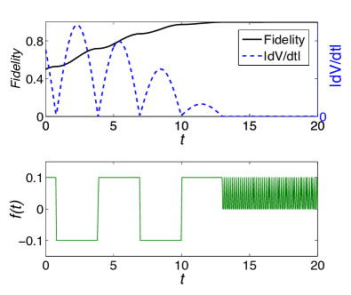
Before analytical calculations and analysis, we present a numerical simulation for the two-level system under control. The system starts with an arbitrary state, $|\psi_{0}\rangle=\cos\frac{\gamma_{0}}{2}|e\rangle+e^{i\phi}\sin\frac{\gamma_{0}}{2}|g\rangle$ with $\gamma_{0}\in(0,\pi)$ and $\phi\in[0,2\pi]$, the target state is $|e\rangle$. Fig. 1 shows the evolution of the fidelity, the control field and the time-derivative of the Lyapunov function with time. In the simulation, we set $\gamma_{0}=\pi/2$, $\phi=-\pi/4$, $\omega=1$ and $S=0.1$. Comparing the time derivative $dV/dt$ and the control field $f(t)$ in Fig. 1, we observe that the control field changes at $dV/dt=0,$ or $\text{Im}(ab^{*})=0$ in Eq. (18). Without loss of generality, $a$ can be set to be a real number, and $\phi$ and $\gamma_{0}$ determine the design of the control field. In addition, we find that the control field alters very quickly when the system is in the vicinity of the target state.

Figure 1: Numerical simulations of the two-level system under the Lyapunov control. $\omega=1$, $S=0.1$, the initial state is chosen as $|\psi(0)\rangle=\frac{1}{\sqrt{2}}[|e\rangle+e^{-i\pi/4}|g\rangle]$.

III.2 Dynamics evolution under control

Assume that the initial state of a two-level system is

$$|\psi_{0}\rangle = \cos\frac{\gamma_{0}}{2}|e\rangle+\sin\frac{\gamma_{0}}{2}e^{i\phi}|g\rangle$$ (29)

$$\equiv a_{0}|e\rangle+b_{0}|g\rangle,$$

where $\gamma_{0}\in[0,\pi]$, and $\phi\in[0,2\pi]$ is the relative phase. With different parameters $\gamma_{0}$ and $\phi$, $|\psi_{0}\rangle$ can represent an arbitrary pure state (ignoring the global phase). Let the target state $|e\rangle$ correspond to the north pole on the Bloch sphere. Since $\text{Im}(a_{0}b_{0}^{*}){=}{-}\frac{\sin\phi\sin\gamma_{0}}{2}$, using the method in (18), the first control field is calculated as,

$$f=\left\{\begin{array}[]{l}S,\ {\text{Im}(a_{0}b_{0}^{*})<}0\ (0{<}\phi{<}\pi),\\ 0,\ {\text{Im}(a_{0}b_{0}^{*})=}0\ (\phi{=}0,\pi),\\ {-}S,\ {\text{Im}(a_{0}b_{0}^{*})>}0\ (\pi{<}\phi{<}2\pi).\end{array}\right.$$ (33)

Assume that this control would last until time $\tau$; i.e., the duration of this control is $\tau$. With this control, the state evolves to

$$|\psi_{\tau}\rangle = [(e^{-iE_{+}\tau}\cos^{2}\frac{\theta}{2}+e^{-iE_{-}\tau}\sin^{2}\frac{\theta}{2})\cos\frac{\gamma_{0}}{2}+\frac{1}{2}(e^{-iE_{+}\tau}-e^{-iE_{-}\tau})\sin\theta\sin\frac{\gamma_{0}}{2}e^{i\phi}]|e\rangle$$ (34)

$$+ [\frac{1}{2}(e^{-iE_{+}\tau}-e^{-iE_{-}\tau})\sin\theta\cos\frac{\gamma_{0}}{2}+(e^{-iE_{-}\tau}\cos^{2}\frac{\theta}{2}+e^{-iE_{+}\tau}\sin^{2}\frac{\theta}{2})\sin\frac{\gamma_{0}}{2}e^{i\phi}]|g\rangle$$

$$\equiv a_{\tau}|e\rangle+b_{\tau}|g\rangle.$$

From the design of the control law in (18), we find that a control field would last until $\text{Im}(a_{\tau}b^{*}_{\tau})$ changes sign. Then $\tau$ can be given by solving $\text{Im}(a_{\tau}b^{*}_{\tau})=0.$ Meanwhile, the sign of $\text{Im}(a_{\tau}b^{*}_{\tau})$ determines the next control field. Simple algebra shows that

$$\text{Im}(a_{\tau}b^{*}_{\tau}) = -\sin\phi\cdot\frac{1}{2}\sin\gamma_{0}(\frac{1}{2}+\frac{1}{2}\cos^{2}\theta)\cdot\cos 2E_{+}\tau-\cos\phi\cdot\frac{1}{2}\sin\gamma_{0}\cdot\cos\theta\cdot\sin 2E_{+}\tau$$ (35)

$$- \sin\phi\cdot\frac{1}{2}\sin\gamma_{0}\cdot\sin^{2}\theta\cdot\frac{1}{2}\cos 2E_{+}\tau+\frac{1}{2}\cos\gamma_{0}\cdot\sin\theta\cdot\sin 2E_{+}\tau.$$

Since $a_{\tau}$ and $b_{\tau}$ are a function of $\phi$, $\gamma_{0}$ and $\theta$, the duration $\tau$ would be determined by these three parameters. Thereby, we arrange our discussions to cover the following cases.

(i) In the case of $\phi\neq 0$, the system would be steered from an arbitrary state to a state on the $xz$ plane on the Bloch sphere, i.e., $|\tilde{\psi}\rangle=\cos\frac{\gamma}{2}|e\rangle+\sin\frac{\gamma}{2}|g\rangle.$ Note that the relative phase is zero, i.e., $\tilde{\phi}=0$.

(ii) In the case of $\phi=0$ and $\gamma_{0}>\theta$, the control field switches slowly between $f=S$ and $f=-S$ until $\gamma_{0}<\theta$. Two situations, $\gamma_{0}\geq 2\theta$ and $\theta<\gamma_{0}<2\theta$, will be separately discussed.

(iii) In the case of $\phi=0$ and $0<\gamma_{0}\leq\theta$, the control becomes inefficient. The control field switches very quickly, and the system may not be steered to the target state $|e\rangle$.

Given an initial state with $\phi\neq 0$ (i.e., case (i)), the first control would steer the system into a state with zero relative phase, i.e., $\tilde{\phi}=0$. The second control process begins with the final state of the first control process (i.e., case (ii)). Using the control law, a state with a zero relative phase yields zero control fields. Hence, for a practical quantum system, a free evolution plays an important role at the beginning of the second control period. It accumulates a relative phase and triggers the second control. Similar control processes would be repeated until $0<\gamma_{0}\leq\theta$ (i.e., case (iii)).

For an arbitrary initial state, the listed cases cover all situations encountered in the method of optimal Lyapunov control used in (18). We will discuss these cases in the next three subsections, where the global phase of the quantum state is neglected throughout the discussions.

III.2.1 The case of $\phi\neq 0$

In this case, the control field is determined by the sign of $\texttt{Im}(a_{0}b_{0}^{*})$. The duration $\tau$ of this control process is determined by $\texttt{Im}(a_{\tau}b^{*}_{\tau})=0$. From Eq. (35), we have

$$\tan 2E_{+}\tau=\frac{\sin\phi}{\sin\theta\cot\gamma_{0}-\cos\phi\cos\theta}.$$ (36)

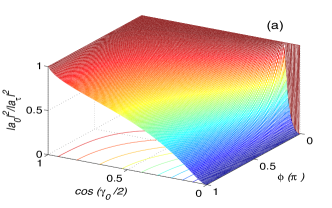
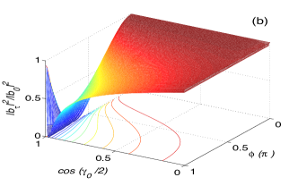
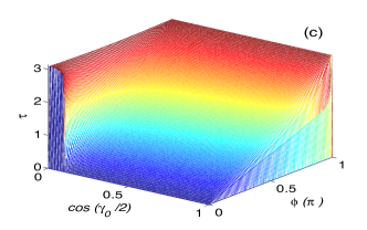
After this control process, the relative phase $\phi$ vanishes. In other words, with an arbitrary state as the initial state, the control would fall into either case (ii) or (iii) after the first control period. Population changes of the system on the two levels after the control can be described by $|a_{0}|^{2}/|a_{\tau}|^{2}$ or $|b_{\tau}|^{2}/|b_{0}|^{2}$, where $a_{\tau}$ and $b_{\tau}$ are given in Eq. (34). $|a_{0}|^{2}/|a_{\tau}|^{2}$ and $|b_{\tau}|^{2}/|b_{0}|^{2}$ versus $\phi$ and $\gamma_{0}$ are shown in Fig. 2-(a) and Fig.2-(b), and the control duration $\tau$ is shown in Fig. 2-(c). Fig. 2 shows that, after the first control process, the amplitude of $|e\rangle$ increases, while the amplitude of $|g\rangle$ decreases.

Figure 2: The state after a control with duration $\tau$ versus the state before the control, with $\omega=1$ and $S=0.1$. (a) is plotted for $|a_{0}|^{2}/|a_{\tau}|^{2}$, (b) for $|b_{\tau}|^{2}/|b_{0}|^{2}$, (c) for the duration $\tau$.

If the initial state can be written in the following form,

$$|\psi_{i}\rangle = \frac{1}{2}[e^{iE_{-}\tau_{i}}+e^{iE_{+}\tau_{i}}+(e^{iE_{+}\tau_{i}}-e^{iE_{-}\tau_{i}})\cos\theta]|e\rangle$$ (37)

$$+ \frac{1}{2}(e^{iE_{+}\tau_{i}}-e^{iE_{-}\tau_{i}})\sin\theta|g\rangle,$$

with $\forall\tau_{i}\in[0,{\pi}/{2E_{+}}]$, the state after the control would be

$$U(\tau_{i})|\psi_{i}\rangle=|e\rangle\langle e|,$$ (38)

i.e., the state can be controlled to the target state by a single control. The states that can be steered to the target state by a single control are shown in Fig. 2-(b) (i.e., the points $(\cos(\gamma_{0}/2),\phi)$ that satisfy $|b_{\tau}|^{2}/|b_{0}|^{2}=0$). A clear demonstration will be presented in Fig. 7-(a) and Fig. 7-(b)). This result will be used to propose an extended technique for optimal Lyapunov quantum control in Sec. IV.

III.2.2 The case of $\phi=0$ and $\gamma_{0}>\theta$

For a state with $\phi=0$, we have

$$|\psi_{1}\rangle_{\pm}=\cos\frac{\gamma_{0}}{2}|e\rangle\pm\sin\frac{\gamma_{0}}{2}|g\rangle,\ \ \gamma_{0}>\theta.$$ (39)

This state may be the resulting state of the first control process.

Note that at this moment $\text{Im}(a_{\tau}b^{*}_{\tau})=0$, and the control field satisfies $f=0$. However, a practical system will acquire a relative phase $\phi$ in an extremely short time due to the free evolution, which would trigger the control. To be specific, assume that the free evolution time is $\delta t^{\prime}\rightarrow 0$. The state after this free evolution is

$$|\psi_{1}^{\prime}\rangle_{\pm}=e^{-\frac{i\omega\delta t^{\prime}}{2}}\cos\frac{\gamma_{0}}{2}|e\rangle\pm e^{\frac{i\omega\delta t^{\prime}}{2}}\sin\frac{\gamma_{0}}{2}|g\rangle.$$ (40)

It turns out that $\text{Im}(a^{\prime}_{\pm}b^{\prime*}_{\pm})=\mp\cos\frac{\gamma_{0}}{2}\sin\frac{\gamma_{0}}{2}\sin{\omega\delta t}$. This triggers a control process with a control field $f=\pm S$. With this control, after $\delta t^{\prime\prime}$, we have

$$\texttt{Im}(a_{\pm}b_{\pm}^{*}) \simeq \mp\sin\omega\delta t^{\prime}\cdot\frac{1}{2}\sin\gamma_{0}\cdot\cos 2E^{+}\delta t^{\prime\prime}$$ (41)

$$\mp \sin(\gamma_{0}-\theta)\sin 2E^{+}\delta t^{\prime\prime}.$$

Here, $\cos\omega\delta t^{\prime}\simeq 1$ has been used. We find that $\texttt{Im}(a_{+}b_{+}^{*})<0$ (and $\texttt{Im}(a_{-}b_{-}^{*})>0$) is kept, since $\gamma_{0}>\theta$. In fact, the control field $f=S$ or $f=-S$ will last for a period of $\tau_{1}$ determined by

$$\mp\sin 2E_{+}\tau_{1}\cdot\frac{1}{2}\sin(\theta-\gamma_{0})=0.$$ (42)

Hence, $\tau_{1}=\pi/2E_{+}$. This control process steers the system from $|\psi_{1}\rangle_{\pm}$ to a state

$$|\psi_{2}\rangle_{\pm} = [(e^{-iE_{+}\tau_{1}}\cos^{2}\frac{\theta}{2}+e^{-iE_{-}\tau_{1}}\sin^{2}\frac{\theta}{2})\cos\frac{\gamma_{0}}{2}$$ (43)

$$+ \frac{1}{2}(e^{-iE_{+}\tau_{1}}-e^{-iE_{-}\tau_{1}})\sin\theta\sin\frac{\gamma_{0}}{2}]|e\rangle$$

$$\pm [\frac{1}{2}(e^{-iE_{+}\tau_{1}}-e^{-iE_{-}\tau_{1}})\sin\theta\cos\frac{\gamma_{0}}{2}$$

$$+ (e^{-iE_{-}\tau_{1}}\cos^{2}\frac{\theta}{2}+e^{-iE_{+}\tau_{1}}\sin^{2}\frac{\theta}{2})\sin\frac{\gamma_{0}}{2}]|g\rangle$$

$$= -i[\cos(\frac{\gamma_{0}}{2}-\theta)|e\rangle\mp\sin(\frac{\gamma_{0}}{2}-\theta)|g\rangle].$$

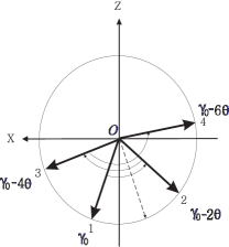
Eq. (43) shows that such a control brings the state closer to the target state. In the Bloch sphere representation, this control reduces the azimuthal angle by $2\theta$, taking the Bloch vector one step closer to the positive $z$ axis (see Fig. 3). The same control would be repeated. After $n$ times, the state evolves to

$$|\psi_{n}\rangle_{\pm} = \cos(\frac{\gamma_{0}}{2}-n\theta)|e\rangle+(-1)^{n}\sin(\frac{\gamma_{0}}{2}-n\theta)|g\rangle,$$ (44)

$$\equiv \cos\frac{\gamma^{\prime}}{2}|e\rangle+(-1)^{n}\sin\frac{\gamma^{\prime}}{2}|g\rangle.$$

Figure 3: Illustration of states after controls on the Bloch sphere. This illustration is for the case of $\gamma_{0}\geq 2\theta$. Each control brings the Bloch vector one step closer to the target by reducing the azimuthal angle. $1(\gamma_{0})\rightarrow 2(\gamma_{0}-2\theta)\rightarrow 3(\gamma_{0}-4\theta)\rightarrow 4(\gamma_{0}-6\theta)\rightarrow\cdots$.

This type of control continues UNTIL $\frac{\gamma_{0}}{2}-n\theta=\frac{\gamma}{2}^{\prime}<\theta$. Next, if $0<\gamma^{\prime}\leq\theta$, this type of control will stop. If $\theta<\gamma^{\prime}<2\theta$, another control would steer the system to the regime $0<\gamma^{\prime}\leq\theta$. Recalling Eq. (44), after $n$ control processes, if a state with $\gamma_{0}>2\theta$ falls into the regime $\theta<\gamma_{0}<2\theta$,

$$|\psi_{1}^{\prime\prime}\rangle_{\pm}=\cos\frac{\gamma_{0}}{2}|e\rangle\pm\sin\frac{\gamma_{0}}{2}|g\rangle,\theta<\gamma_{0}<2\theta,$$ (45)

we can employ the same analysis as that in the case of $\gamma_{0}>2\theta$ to find a control that will steer the initial state $|\psi_{1}^{\prime\prime}\rangle_{\pm}$ to

$$|\psi_{2}^{\prime\prime}\rangle_{\pm} = e^{i\epsilon}\Big{[}\cos\frac{|2\theta-\gamma_{0}|}{2}|e\rangle\pm\sin\frac{|2\theta-\gamma_{0}|}{2}|g\rangle\Big{]}$$ (46)

$$= \cos\frac{\gamma}{2}^{\prime\prime}|e\rangle\pm\sin\frac{\gamma}{2}^{\prime\prime}|g\rangle.$$

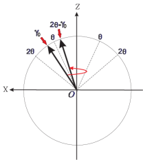
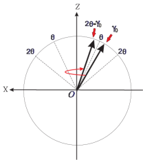
It is clear that $0<|2\theta-\gamma_{0}|<\theta$ since $\theta<\gamma_{0}<2\theta$. Namely, the states finally fall into the regime $0<\gamma_{0}\leq\theta$ (see Fig. 4). Hence, using the second type of control processes, the state can be driven to

$$|\psi^{\prime}_{n}\rangle_{\pm}=\cos\frac{\gamma}{2}^{\prime}|e\rangle\pm\sin\frac{\gamma}{2}^{\prime}|g\rangle,\ (0<\gamma^{\prime}\leq\theta).$$ (47)

Figure 4: Illustration of Bloch vectors before and after the control for the case $\phi=0$ and $\theta<\gamma_{0}<2\theta$. (a) is for initial state $|\psi_{1}^{\prime\prime}\rangle_{+}$, while (b) for initial state $|\psi_{1}^{\prime\prime}\rangle_{-}$.

If

$$\frac{\gamma_{0}}{2}-n\theta=0,(n=1,2,...),$$ (48)

the system can be steered exactly to the target state by $n$ controls. The number of controls $n$ can be given by

$$\theta=\frac{\gamma_{0}}{2n}\ \ \ \Leftrightarrow\ \ \ \arctan\frac{2f}{\omega}=\frac{\gamma_{0}}{2n}.$$ (49)

On the other hand, given a number of controls $n_{0}$, we can calculate the control strength such that the system can be steered exactly to the target state by $n_{0}$ times of control processes

When (48) is not satisfied, we consider a new control process for the state in (47) in the next subsection.

III.2.3 The case of $\phi=0$ and $0<\gamma_{0}\leq\theta$

Now we discuss the control starting with a state,

$$|\psi_{1}\rangle_{\pm}=\cos\frac{\gamma_{0}}{2}|e\rangle\pm\sin\frac{\gamma_{0}}{2}|g\rangle,\ \ 0<\gamma_{0}\leq\theta.$$ (50)

The control field is zero at the beginning by the control law. After an infinitesimal $\delta t^{\prime}\rightarrow 0$ free evolution, a control with control field $f=\pm S$ is triggered. After a period of $\delta t^{\prime\prime}$, we have,

$$\texttt{Im}(a_{\pm}b_{\pm}^{*}) = \pm\frac{1}{2}\sin\omega\delta t^{\prime}\cdot\sin\gamma_{0}\cdot\cos 2E^{+}\delta t^{\prime\prime}$$ (51)

$$\mp \sin(\gamma_{0}-\theta)\sin 2E^{+}\delta t^{\prime\prime}.$$

A careful examination shows that this is different from Eq. (41), because the sign of $\texttt{Im}(a_{\pm}b_{\pm}^{*})$ in Eq. (41) does not change after the infinitesimal control, and the control would last until the azimuthal angle lost $2\theta$, whereas in the case of $\gamma_{0}<\theta$, the control can not last for such a long time since $\sin(\gamma_{0}-\theta)<0$. In fact, the control field switches very quickly in this case. The (infinitesimal) duration of the control $\delta t^{\prime\prime}$ satisfies,

$$\tan 2E_{+}\delta t^{\prime\prime}=\frac{\sin\omega\delta t^{\prime}}{\sin\theta\cot\gamma_{0}-\cos\omega\delta t^{\prime}\cos\theta}.$$ (52)

After this duration, the system evolves to $|\psi\rangle=\cos\frac{\gamma}{2}^{\prime}|e\rangle+\frac{\gamma}{2}^{\prime}|g\rangle$ with $0<\gamma^{\prime}\leq\theta$ again. Since the control time $\delta t^{\prime\prime}$ are determined by the free-evolution time $\delta t^{\prime}$, therefore, $\delta t^{\prime}$ can not be ignored for a practical system.

For a very small duration, the control could drive the system closer to the target, since

$$\frac{|\cos\frac{\gamma}{2}^{\prime}|^{2}}{|\cos\frac{\gamma_{0}}{2}|^{2}} \simeq 1+\frac{(\omega\delta t^{\prime})^{2}\sin^{2}\frac{\gamma_{0}}{2}\sin\theta[\sin(\theta-\gamma_{0})+\frac{\sin\gamma_{0}}{2}]}{\sin^{2}(\theta-\gamma_{0})}$$ (53)

$$= 1+A(\gamma_{0})\delta t^{\prime 2}>1,$$

where we have neglected the high order terms of $\delta t^{\prime}$. Eq. (53) tells us that in this infinitesimal control, the convergence of the system towards the target state could depend on the free evolution time $\delta t^{\prime}$. Hence, an additional free evolution may help improve the effectiveness of the control law in (18).

III.3 Control limit and strength of control fields

As mentioned above, the state of the system can be described by $\gamma_{0}$ and $\phi$. When $\gamma_{0}$ satisfies $0<\gamma_{0}\leq\theta$, the control becomes inefficient, i.e., the control fields switch very quickly but the system may not evolve towards the target. We refer to this control as fast-switching control (FSC), and the controls before this as slow switching controls (SSC). With this knowledge, one may wonder, if we can stop the control before $\gamma_{0}$ enters the regime $0<\gamma_{0}\leq\theta$. To answer this question, we examine the fidelity achieved by the slow-switching controls.

Denoting $\gamma_{f}$ the azimuthal angle reached by the SSC, we find that

$$F=\cos^{2}\frac{\gamma_{f}}{2}\geq\cos^{2}\frac{\theta}{2}=\frac{1}{2}+\frac{1}{2\sqrt{1+(2S/\omega)^{2}}}.$$ (54)

Fig. 5 shows the fidelity of the SSC versus the strength of the control field and the initial state.

Figure 5: The fidelity of SSC versus the strength of the control field. The solid line in (a) plots the the lower bound of the fidelity reached by SSC, given in Eq. (54), while the dot-solid line is for the fidelity of SSC with initial state, $1/\sqrt{2}(|e\rangle+|g\rangle)$. Figure (b) shows the fidelity of SSC versus the strength of the control fields and initial states, $|\psi(0)\rangle=\cos\frac{\gamma}{2}|e\rangle+\sin\frac{\gamma}{2}|g\rangle$, $\gamma\in[0,\pi]$.

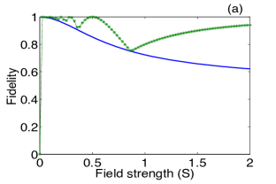
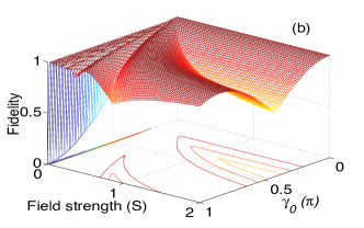
We find from Fig. 5 that the smaller the strength of the control field is, the larger the fidelity of the SSC could be. Note that small control strength needs more alternations (e.g., from $-S$ to $S$) in the control fields.

For an arbitrary initial state, $|\psi(0)\rangle=\cos\frac{\gamma}{2}|e\rangle+e^{i\phi}\sin\frac{\gamma}{2}|g\rangle$, the resulting state of the system after SSC becomes,

$$|\psi_{f}\rangle=\left\{\begin{array}[]{l}\cos\frac{2\theta-\gamma^{\prime}}{2}|e\rangle+\sin\frac{2\theta-\gamma^{\prime}}{2}|g\rangle,\ (\theta<\gamma^{\prime}\leq 2\theta),\\ \cos\frac{\gamma^{\prime}}{2}|e\rangle+\sin\frac{\gamma^{\prime}}{2}|g\rangle,\ (0<\gamma^{\prime}\leq\theta),\\ \end{array}\right.$$ (57)

where,

$$\gamma^{\prime}=\gamma-2n_{max}\theta,$$

$$\cos\frac{\gamma}{2}=(e^{-iE_{+}\tau}\cos^{2}\frac{\theta}{2}+e^{-iE_{-}\tau}\sin^{2}\frac{\theta}{2})\cos\frac{\gamma_{0}}{2}$$

$$\ \ \ \ \ \ \ \ +\frac{1}{2}(e^{-iE_{+}\tau}-e^{-iE_{-}\tau})\sin\theta\sin\frac{\gamma_{0}}{2}e^{i\phi},$$

$$\tan 2E_{+}\tau=\frac{\sin\phi}{\sin\theta\cot\gamma_{0}-\cos\phi\cos\theta}.$$ (58)

Here, $n_{max}$ denotes the number of SSC which depends not only on the initial states but also on the strength of the control. With these resulting states, we can calculate the fidelity reached by the SSC. Stronger control fields usually lead to smaller fidelity of SSC and less number of controls (see Fig. 6).

Figure 6: Fidelity of SSC as a function of initial states, $|\psi(0)\rangle=\cos\frac{\gamma_{0}}{2}|e\rangle+e^{i\phi}\sin\frac{\gamma_{0}}{2}|g\rangle$, (a) and (b) are for different control strengths, (a) $S=0.1$; (b) $S=0.05$.

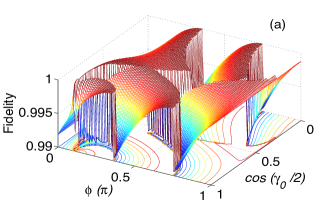
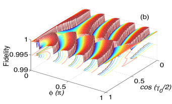
From Fig. 6, we also find that with fixed strength of the control field, the SSC itself can drive some initial states into the target state precisely. Alternatively, for an specific initial state, we can find a control strength that steers it to the target with fidelity one.

IV Extended technique

As discussed in the last section, the control law in (18) may become inefficient when the system is very close to the target state. If we stop the controls before the inefficient FSC, the control fidelity can not reach a desirable value. In this section, we propose an extended technique to improve the optimal Lyapunov quantum control in hou2012 .

Recall that an additional free evolution may enhance the efficiency of the control. We combine free evolution and external control into the extended technique where different controls are used for a state with $\texttt{Im}(ab^{*})=0$ according to whether $|a|^{2}<\cos^{2}\theta$ or not. For a state close to the target ($|a|^{2}>\cos^{2}\theta$), we implement an additional free evolution with $\Delta t$, while for a state far from the target, we take the same control law in (18). Suitable design of $\Delta t$ can steer the system to the target state.

In Subsection III.B, we find that if an initial state satisfies,

$$|\psi_{i}\rangle = \frac{1}{2}[e^{iE_{-}t}+e^{iE_{+}t}+(e^{iE_{+}t}-e^{iE_{-}t})\cos\theta]|e\rangle$$ (59)

$$+ \frac{1}{2}(e^{iE_{+}t}-e^{iE_{-}t})\sin\theta|g\rangle,$$

with parameter $t$ in $[0,{\pi}/{2E_{+}}]$, the state can be steered into the target state by a single control.

To see clearly what type of states can be steered to the target by a single control, we rewrite the state in Eq. (59) in the following form,

$$|\psi_{i}\rangle{=}e^{i\pi}\Big{[}e^{i\phi^{\prime}}\sqrt{1{-}\sin^{2}E_{+}t\sin^{2}\theta}|e\rangle+\sin E_{+}t\sin\theta|g\rangle\Big{]},$$

where $\phi^{\prime}$ is defined by

$$\tan\phi^{\prime}=\frac{\cos E_{+}t}{\sin E_{+}t\cos\theta}.$$ (61)

Figure 7: Figure (a) is an enlarged part of Fig.2-(b). (b) shows the states ( characterized by $\gamma$ and $\phi$ ) that can be steered to the target by a single control. (c) $|b_{\tau}|^{2}/|b_{0}|^{2}$ versus $\cos\frac{\gamma}{2}$ with $\phi=\pi/2$ in figure (a).

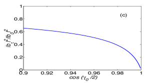
Since $\cos^{2}\theta\leq 1-\sin^{2}E_{+}t\sin^{2}\theta\leq 1$, and $1-\sin^{2}E_{+}t\sin^{2}\theta$ represents the probability to obtain the target state $|e\rangle$ when making a measurement, any state $a|e\rangle+b|g\rangle$ with $|a|^{2}>\cos^{2}\theta$ can be controlled to the target state by a single control, provided that $\phi^{\prime}$ satisfies the condition in (61). It is worth mentioning that $\phi^{\prime}$ is the relative phase, which can be manipulated by changing the free evolution time to any required value.

As shown in Subsection III.C, by the slow-switching control, the population of the system on the target state can reach at least $\cos^{2}\frac{\theta}{2}$ . Since

$$\cos^{2}\theta\leq\cos^{2}\frac{\theta}{2}\leq 1,\ \ \ \theta\in[0,\frac{\pi}{2}],$$ (62)

we conclude that all states after the slow-switching controls can be steered to the target by a single control. The free evolution time needed to accumulate the relative phase is

$$t^{\prime\prime}=\frac{\phi^{\prime\prime}}{2\omega}=\frac{1}{2\omega}\arctan\frac{\cos E_{+}\tau^{\prime}}{\sin E_{+}\tau^{\prime}\cos\theta},$$ (63)

where,

$$\tau^{\prime}=\frac{1}{E_{+}}{\arcsin\frac{\sin\frac{\gamma}{2}}{\sin\theta}},\ \ \ \tau^{\prime}\in[0,\frac{\pi}{2E_{+}}].$$ (64)

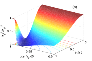
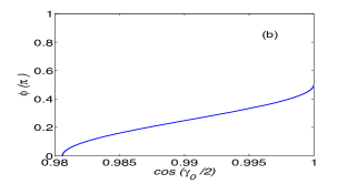
When an initial state $(\cos\frac{\gamma}{2}|e\rangle+\sin\frac{\gamma}{2}|e\rangle)$ is very close to the target state, i.e., $\cos^{2}\frac{\gamma}{2}\rightarrow 1$, by Eq. (63) and Eq. (64), we estimate that the relative phase required for the single control is $\phi^{\prime}\rightarrow\frac{\pi}{2}$, corresponding to a free-evolution time $t^{\prime\prime}\rightarrow\frac{\pi}{4\omega}$. This result is confirmed by Fig.7-(b), and it is in agreement with the following relationship

$$\frac{|b_{\tau}|^{2}}{|b_{0}|^{2}}\simeq\cos^{2}\phi^{\prime}=\frac{1+\cos(2\phi^{\prime})}{2},$$ (65)

since $|b_{\tau}|^{2}$ can be expanded in a neighborhood of $|b_{0}|^{2}$ when control starts with a state very close to its target, i.e., $b_{0}$ is very small.

In the case of small $b_{0}$, i.e., when $\phi^{\prime}\rightarrow\frac{\pi}{2}$,

$$\frac{|b_{\tau}|^{2}}{|b_{0}|^{2}}\rightarrow 0,$$

with $\cos\frac{\gamma}{2}\rightarrow 1$. This means if we let the system acquire a relative phase $\phi^{\prime}=\pi/2$, the Lyapunov control would become more effective when the system is very close to the target state (see Fig.7-(c)).

V conclusions

We have studied the optimal Lyapunov control by an exactly solvable two-level model in this paper. We found that the convergence time and the control fidelity are related to the strength of control fields. When the system is close to the target state, the optimal Lyapunov control in (18) may become inefficient, i.e., the system under control may not converge to the target state. To overcome this difficulty, we extended the control law by combining free evolution and external control. With this extended technique, the state in the vicinity of target state can be controlled to the target by a single control.

References

- (1) M. A. Nielsen and I. L. Chuang, Quantum Computation and Quantum Information(Cambridge University Press, 2000)
- (2) D. D’Alesandro, Introduction to Quantum Control and Dynamics, Taylor and Francis Group, Boca Raton, 2007.
- (3) H. M. Wiseman and G. J. Milburn, Quantum Measurement and Control, Cambridge University Press, 2010.
- (4) D. Dong, J. Lam, and I. R. Petersen, Int. J. Control 83, 206 (2010).
- (5) D. Dong and I. R. Petersen, IET Control Theory Appl. 4, 2651 (2010).
- (6) C. Altafini, Quantum Information Process 6, 9 (2007); C. Altafini, IEEE Trans. Autom. Control, 52, 2019 (2007).
- (7) S. Grivopoulos, and B. Bamieh, Proceedings of the 42nd IEEE Conference on Decision and Control (2003).
- (8) M. Mirrahimi, P. Rouchon, and G. Turinici, Automatica 41, 1987 (2005).
- (9) X. Wang and S. G. Schirmer, IEEE Transactions on Automatic Control 55, 2259 (2010); X. Wang and S. G. Schirmer, ENOC 2008, Saint Petersburg, Russia, June 30 July 4 (2008).
- (10) S. Kuang and S. Cong, Automatica 44, 98 (2008); S. Cong, and S. Kuang, Acta Automatica Sinica 33, 28 (2007).
- (11) J. M. Coron, A. Grigoriu, C. Lefter, and G. Turinici, New J. Phys. 11, 105034 (2009).
- (12) K. Beauchard, J. M. Coron, M. Mirrahimi, and P. Rouchon, Systems and Control Letters 56, 388 (2007).
- (13) X. Wang and S. G. Schirmer, Phys. Rev. A 80, 042305 (2009).
- (14) W. Wang, L. C. Wang, and X. X. Yi, Phys. Rev. A 82, 034308 (2010).
- (15) X. X. Yi, S. L. Wu, Chunfeng Wu, X. L. Feng, and C. H. Oh, J. Phys. B: At. Mol. Opt. Phys. 44, 195503 (2011).
- (16) X. X. Yi, B. Cui, Chunfeng Wu, and C. H. Oh, J. Phys. B: At. Mol. Opt. Phys. 44, 165503 (2011).
- (17) S. C. Hou, M. A. Khan, X. X. Yi, D. Dong, and I. R. Petersen, Phys. Rev. A 86, 022321 (2012).
- (18) X. X. Yi, X. L. Huang, Chunfeng Wu, and C. H. Oh, Phys. Rev. A 80, 052316 (2009).
- (19) W. Wang, L. C. Wang, and X. X. Yi, Phys. Rev. A 82, 034308 (2010).