Multi-fidelity Stochastic Collocation \authorheadRaissi & Seshaiyer \corrauthorPadmanabhan Seshaiyer \corremailpseshaiy@gmu.edu \corrurlhttp://math.gmu.edu/ pseshaiy/
A multi-fidelity stochastic collocation
method for parabolic PDEs with
random
input data
Abstract
Over the last few years there have been dramatic advances in our understanding of mathematical and computational models of complex systems in the presence of uncertainty. This has led to a growth in the area of uncertainty quantification as well as the need to develop efficient, scalable, stable and convergent computational methods for solving differential equations with random inputs. Stochastic Galerkin methods based on polynomial chaos expansions have shown superiority to other non-sampling and many sampling techniques. However, for complicated governing equations numerical implementations of stochastic Galerkin methods can become non-trivial. On the other hand, Monte Carlo and other traditional sampling methods, are straightforward to implement. However, they do not offer as fast convergence rates as stochastic Galerkin. Other numerical approaches are the stochastic collocation (SC) methods, which inherit both, the ease of implementation of Monte Carlo and the robustness of stochastic Galerkin to a great deal. In this work we propose a novel enhancement to stochastic collocation methods using deterministic model reduction techniques. Linear parabolic partial differential equations with random forcing terms are analysed. The input data are assumed to be represented by a finite number of random variables. A rigorous convergence analysis, supported by numerical results, shows that the proposed technique is not only reliable and robust but also efficient.
keywords:
collocation, stochastic partial differential equations, sparse grid, smolyak algorithm, finite element, proper orthogonal decomposition, multi-fidelity1 Introduction
The effectiveness of stochastic partial differential equations (SPDEs) in modelling complicated phenomena is a well-known fact. One can name wave propagation [1], diffusion through heterogeneous random media [2], randomly forced Burgers and NavierStokes equations (see e.g [3, 4, 5, 6] and the references therein) as a couple of examples. Currently, Monte Carlo is by far the most widely used tool in simulating models driven by SPDEs. However, Monte Carlo simulations are generally very expensive. To meet this concern, methods based on the Fourier analysis with respect to the Gaussian (rather than Lebesgue) measure, have been investigated in recent decades. More specifically, Cameron–Martin version of the Wiener Chaos expansion (see, e.g. [7, 8] and the references therein) is among the earlier efforts. Sometimes, the Wiener Chaos expansion (WCE for short) is also referred to as the Hermite polynomial chaos expansion. The term polynomial chaos was coined by Nobert Wiener [9]. In Wieners work, Hermite polynomials served as an orthogonal basis. The validity of the approach was then proved in [7]. There is a long history of using WCE as well as other polynomial chaos expansions in problems in physics and engineering. See, e.g. [10, 11, 12, 13], etc. Applications of the polynomial chaos to stochastic PDEs considered in the literature typically deal with stochastic input generated by a finite number of random variables (see, e.g. [14, 15, 16, 17]). This assumption is usually introduced either directly or via a representation of the stochastic input by a truncated Karhunen–Loève expansion. Stochastic finite element methods based on the Karhunen–Loève expansion and Hermite polynomial chaos expansion [15, 14] have been developed by Ghanem and other authors. Karniadakis et al. generalized this idea to other types of randomness and polynomials [18, 16, 19]. The stochastic finite element procedure often results in a set of coupled deterministic equations which requires additional effort to be solved. To resolve this issue, stochastic collocation (SC) method was introduced. In this method one repeatedly executes an established deterministic code on a prescribed node in the random space defined by the random inputs. The idea can be found in early works such as [20, 21]. In these works mostly tensor products of one-dimensional nodes (e.g., Gauss quadrature) are employed. Tensor product construction despite making mathematical analysis more accessible (cf. [22]) leads to the curse of dimensionality since the total number of nodes grows exponentially fast as the number of random parameters increases. In recent years we are experiencing a surge of interest in the high-order stochastic collocation approach following [23]. The use of sparse grids from multivariate interpolation analysis, is a distinct feature of the work in [23]. A sparse grid, being a subset of the full tensor grid, can retain many of the accuracy properties of the tensor grid. While keeping high-order accuracy, it can significantly reduce the number of nodes in higher random dimensions. Further reduction in the number of nodes was pursued in [24, 25, 26, 27]. Applications of these numerical methods take a wide range. Here we mention some of the more representative works. It includes Burgers’ equation [28, 29], fluid dynamics [30, 31, 32, 33, 16], flow-structure interactions [34], hyperbolic problems [35, 36, 37], model construction and reduction [38, 39, 40], random domains with rough boundaries [41, 42, 43, 44], etc.
Along with an attempt to reduce the number of nodes used by sparse grid stochastic collocation, one can try to employ more efficient deterministic algorithms. The current trend is to repeatedly execute a full-scale underlying deterministic simulation on prescribed nodes in the random space. However, model reduction techniques can be employed to create a computationally cheap deterministic algorithm that can be used for most of the grid points. This way we can limit the employment of an established while computationally expensive algorithm to only a relatively small number of points. A similar method is being used by K. Willcox and her team but in the context of optimization [45]. “Multifidelity", which we also adopt, is the term they employed in their work. Reduced order modelling, using proper orthogonal decompositions (POD) along with Galerkin projection, for fluid flows has seen extensive applications studied in [46, 47, 48, 49, 50, 51, 52, 53, 54, 55]. Proper orthogonal decomposition (POD) was introduce in Pearson [56] and Hotelling [57]. Since the work of Pearson and Hotelling, many have studied or used POD in a range of fields such as oceanography [58], fluid mechanics [46, 48], system feedback control [59, 60, 61, 62, 63, 64], and system modeling [49, 52, 54, 65]. In this work we analyse linear parabolic partial differential equations with random forcing terms. We propose a novel method which dramatically decreases the computational cost. The idea of the method is very simple. For each point of the stochastic parameter domain we search to see if the resulting deterministic problem is already solved for a sufficiently close problem. If yes, we use the solution to the nearby problem to create POD basis functions and we employ POD-Galerkin method to solve the original problem. We provide a rigorous convergence analysis for our proposed method. Finally, it is shown by numerical examples that the results of numerical computation are consistent with theoretical conclusions.
2 Problem definition
Let be a bounded, connected and polygonal domain and denote a complete probability space with sample space , which corresponds to the set of all possible outcomes. is the -algebra of events, and is the probability measure. In this section, we consider the stochastic linear parabolic initial-boundary value problem: find a random field , such that -almost surely the following equations hold:
| in | |||||
| on | (1) | ||||
| on |
In order to guarantee the existence and uniqueness of the solution of (2), we assume that the random forcing field satisfies:
| (2) |
Following [22] and inspired by the truncated KL expansion [66], we make the assumption that the random field depends on a finite number of independent random variables. More specifically,
| on | (3) |
where and . Lets define the space,
where denotes an -dimensional random vector over . We also define the Hilbert space,
with the inner product given by:
A function is called a weak solution of problem (2) if:
| (4) |
and -almost surely . The existence and uniqueness of the solution of problem (4) is a direct consequence of assumption (2) on ; see [67].
Let denote the image of the random variable , for , and . We also assume that the distribution measure of is absolutely continuous with respect to the Lebesgue measure. Thus, there exists a joint density function for . Hence, we can use instead of , where is the -dimensional Borel space. Analogous to the definitions of and we can define
and
with inner product
where
The weak solution of problem (2), using the finite dimensional noise assumption (3), is of the form . Therefore, the weak formulation (4) can be equivalently expressed as finding such that -almost everywhere in , , and
| (5) |
For each fixed , the solution to (5) can be viewed as a mapping . In order to emphasize the dependence on the variable , we use the notations and . Hence, we achieve the following equivalent settings: find such that -almost everywhere in , , and
| (6) |
Note that there may exist a -zero measure set in which (6) is not satisfied. Therefore, from a computational perspective, if a point is chosen, the resulting solution of (6) is not the true solution of the original equation. However, the computation of the moments of the solution does not suffer from this disadvantage.
3 Multi-fidelity Collocation method
In this section, we apply our multi-fidelity stochastic collocation method to the weak form (6). Let be a finite dimensional subspace of given by , where is a standard finite element space and is the span of tensor product polynomials with degree at most . The goal is to find a numerical approximation to the solution of (6) in the finite dimensional subspace . Choose to be a small real number. The procedure for solving (6) is divided into two parts:
-
1.
Fix , and search the -neighbourhood of . If problem (6) is not already solved for any nearby problem with , solve problem (6) using a regular backward Euler finite element method at and let . In contrast, if equation (6) is already solved for some points in , choose one of them and call it . In either case, use the solution at to find a small number of suitable orthonormal basis functions using proper orthogonal decomposition (POD) method. Now use Galerkin projection on to the subspace to find
such that
(7) and , where is the number of time steps, and denotes the time step increments. It is worth mentioning that denotes the -inner product. Note that we are employing a backward Euler scheme to discretize time.
-
2.
Collocate (7) on zeros of suitable orthogonal polynomials and build the interpolated discrete solution
(8) using
(9)
where the functions can be taken as Lagrange polynomials. Using this formula, as described in [22], mean value and variance of can also be easily approximated.
3.1 Proper orthogonal decomposition
In this section, we choose a fixed and drop the dependence of equation (6) on , for notational conveniences. Therefore, we consider the problem of finding such that:
| (10) |
and , for all . Note that . Let , where denotes the time step increments. Assume to be a uniformly regular family of triangulation of (see [68, 69]). The finite element space is taken as
where and is the space of polynomials of degree on . Write , and let denote the fully discrete approximation of resulting from solving the problem of finding such that and for ,
| (11) |
It is easy to prove that problem (11) has a unique solution , provided that (see [68]). One can also show that if and , the following error estimates hold:
| (12) |
where denotes the -norm and indicates a positive constant independent of the spatial and temporal mesh sizes, possibly different at distinct occurrences.
For the so-called snapshots , , where , let
Assume at least one of is non-zero, and let be an orthonormal basis of with . Therefore, for each we will have:
| (13) |
where . {defi} The POD method consists of finding an orthonormal basis such that for every , the following problem is solved
| (14) |
A solution of this minimization problem is known as a POD basis of rank . Let us introduce the correlation matrix given by
| (15) |
The following proposition (see [46, 51, 52]) solves problem (14).
Proposition 1.
Let denote the positive eigenvalues of and the associated orthonormal eigenvectors. Then a POD basis of rank is given by
| (16) |
where denotes the -th component of the eigenvector . Furthermore, the following error formula holds:
| (17) |
Let , and consider the problem of finding such that and for ,
| (18) |
If is a uniformly regular triangulation and is the the space of piecewise linear functions, the total degrees of freedom for problem (11) is , where is the number of vertices of triangles in , while the total of degrees of freedom for problem (18) is (where ). The following proposition, proved in [70], gives us an error estimate on the solution of problem (18).
Proposition 2.
Proposition 3.
Now, with a slight misusing of notation, we assume that the function is given by , where is the function employed in equation (6), and consider the following problem: find such that , for all , and
| (21) |
Note that since and under the assumption that is Lipschitz continuous on , we get that , where is the Lipschitz constant. Also, note that we are slightly misusing the symbol to denote both the function employed in equation (6) and the function used in equation (10). Let us also consider the following problem: find such that and for ,
| (22) |
Note that equations (22) and (7) are identical, using the fact that we are using . Our aim is to find an estimate for . First we need to prove two lemmas. {lemm} Let be the solution of problem (21) and let be the solution of problem (10), then we have:
| (23) |
Proof 3.1.
let and subtract equations (10) and (21) to get:
| (24) |
with , for all . Letting and integrating equation (24) from 0 to , we get:
This results in
Therefore,
| (25) |
Now we need to bound . For this, we integrate (24) once again but this time upto , and use the Poincaré inequality , for each , to get:
Therefore,
Thus,
Choose such that , and let
Proof 3.2.
4 Error analysis
In this section, we carry out an error analysis for the multi-fidelity collocation method introduced in section 3 for problem (6). In [22], the authors showed that if the solution of (6) is analytic with respect to the random parameters, then the collocation scheme (9) attains an exponential error decay for with respect to each . The convergence proof in [22] applies directly to our case. Therefore, our main task is to prove the analyticity property of the POD solution eith respect to each random variable . We will then only state the corresponding convergence result. In the following we impose similar restrictions on as in [22, 71], \ie is continuous with respect to each element and that it has at most exponential growth at infinity, whenever the domain is unbounded. Moreover, we assume that joint density function behaves like a Gaussian kernel at infinity. In order to make it precise, we introduce the weight function , where
and the space
where is a Banach space. In what follows, we assume that and the joint probability density satisfies
| (29) |
for some constant , with being strictly positive if is unbounded and zero otherwise. Under these assumptions, the following proposition is immediate; see [22].
Proposition 4.
Furthermore, we have the following regularity result. {lemm} The following energy estimate holds:
where is the Poincaré canstant.
Proof 4.1.
Similar to the proof of lemma 3.1.
4.1 Analyticity with respect to random parameters
We prove that the solution of equation (22) is analytic with respect to each random parameter , whenever is infinitely differentiable with respect to each component of . To do this, we introduce the following notations as in [22, 71]:
We first make the additional assumption that for every , there exists such that
| (30) |
Under the finite dimensional noise assumption (3), is represented by a truncated linear or nonlinear expansion so that assumption (30) holds. For example, consider a truncated KL expansion for random forcing term given by
| (31) |
We have
Therefore, we can set , and observe that definition (31) satisfies assumption (30). Moreover, the random forcing defined in (31), satisfies the Lipschitz continuity assumption of remark 3.1. {lemm} Under assumption (30), if the solution is considered as a function of , \ie, then the -th derivative of with respect to satisfies
| (32) |
where depends on , and the Poincaré constant .
Proof 4.2.
We will immediately obtain the following theorem, whose proof closely follows the proof of theorem 4.4 in [71]. {theo} Under assumption (30), the solution considered as a function of , admits an analytic extension , , in the region of complex plane
where .
Proof 4.3.
For each we define the power series as
Thus,
where is a function of , and the constant is a function of . The series is convergent for all , provided that . Therefore, the function admits an analytic extension in the region .
4.2 Convergence analysis
Our goal is to provide an estimate for the total error in the norm , for each . The error splits naturally into . Recall that and is given by (9). We can estimate the interpolation error by repeating the same procedure as in [22], using the analyticity result of theorem 4.2. All details about the estimates of the interpolation error can be found in section 4 of [22] and the references cited therein. Therefore we state the following theorem without proof. {theo} Under assumption (30), there exist positive constants and that are independent of , and such that
| (33) |
where
and
where is the minimum distance between and the nearest singularity in the complex plane, as defined in theorem 4.2, and is defined in assumption (29). {rema}[Convergence with respect to the number of collocation points] For an isotropic full tensor-product approximation, \ie, the number of collocation points is given by . Thus, one can easily obtain the following error bound with respect to ; see [71].
| (36) |
where as in theorem 4.2. The constant depends on and . {rema}[Extensions to sparse grid stochastic collocation methods] Note that the convergence as shown in (36) becomes slower as the dimension increases. This slow-down effect as a result of increase in dimension is called the curse of dimensionality. For large values of , sparse grid stochastic collocation methods [72, 26], specially adaptive and anisotropic ones, \eg[25, 27] are more effective in dealing with this problem. Our analyticity result (theorem 4.2) combined with the analysis in [72, 26, 25, 27], can easily lead to the derivation of error bounds for sparse grid approximations. For instance, for an isotropic Smolyak approximation [72, 26] with a total of sparse grid points, the error can be bounded by
Here, we will give a short description of the isotropic Smolyak algorithm. More detailed information can be found in [73, 26]. Assume . For , let be a sequence of interpolation operators given by equation (9). Define and . Now for , let
| (37) |
where is a non-negative integer. is the Smolyak operator, and is known as the sparse grid level. Now we need to find error bounds for the deterministic part of our algorithm in the norm, \ie. First, note that according to (29), the joint density function behaves like a Gaussian kernel at infinity. Therefore, in practice we are literally dealing with a compact random parameter set , since we can approximate with a large enough compact set. So from now on we assume that is compact. We know that . Thus, using the compactness assumption on , there exist and such that . Letting , we can write . {theo} Under the Lipschitz continuity (see remark 3.1) assumption, the exist constants and such that
| (38) |
Proof 4.4.
Let us first integrate the the last term in estimate (28). Thus, we have
Now letting , and assuming , we get the following upper bound for the above expression:
Letting , we get the last term in (38). The first three terms of (38) can also be easily computed by integrating the first three terms of (28). We will get the same expressions for the constants as above.
Note that due to the way that the POD method works, the constant is so small that the term has a very little effect on the error. Combining (33) and (38), we will finally get the following total error estimate. {theo} Under assumption (30) and the Lipschitz continuity (see remark 3.1) assumption , there exist positive constants and that are independent of and , and there exist constants such that
| (39) |
where and are the same as the ones in theorem 4.2. {rema} In some cases, one might be interested in estimating the expectation error, \ie. This can be easily achieved by observing that:
| (40) | |||||
5 Numerical experiments
In this section, we provide a computational example to illustrate the advantages of multi-fidelity stochastic collocation method. Specifically, we consider problem (2) with , , and the forcing term being given by:
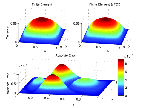
The real-valued random variables , are supposed to be independent and have uniform distributions . In the followings, we let . We employ the sparse grid stochastic collocation method introduced in remark 4.2 with sparse grid level . We use the Clenshaw-Curtis abscissas (see [74]) as collocation points. These abscissas are the extrema of Chebyshev polynomials. We divide the spatial domain into small squares with side length , and then we connect the diagonals of the squares to divide each square into two triangles. These triangles consist the triangulation , with . Take as the time step increment. We use all of the time steps to form the snapshots. We employ POD basis functions. In the following, we compare the solution resulting from a regular isotropic sparse grid stochastic collocation method which only uses the finite element method, with the hybrid multi-fidelity method proposed in this paper which employs both finite element and POD methods. In figure 1, we compare the expected values resulting from the multi-fidelity method and a regular sparse grid stochastic collocation method. We take . Recall that for each our method searches the neighbourhood of to check whether for some problem (6) is already solved. If a nearby problem (at ) is found to be solved by finite element method, our algorithm uses this information to create POD basis functions and solves problem (6) at using Galerkin-POD method which is computationally much cheaper than finite element. Moreover, figure 2 compares variances of solutions resulting from the two methods.

resulting from a regular sparse grid method (top left)
and the multi-fidelity method with (top right).
resulting from a regular sparse grid method (top left)
and the multi-fidelity method with (top right).
Figures 3 and 4, show the convergence patterns of expectations and variances of solutions with regard to , respectively. These results validate our theoretical estimates of previous sections. We are actually comparing our multi-fidelity method with a regular sparse grid stochastic method. Note that for small enough (less than the shortest distance between the collocation points) we get the regular sparse grid method back. Therefore the error is zero for such a small .
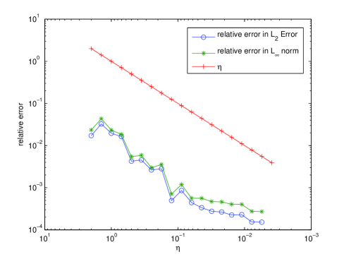
solutions with respect to .
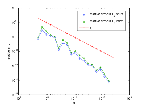
with respect to .

Figure 5 demonstrates how the number of times that the finite element code is employed increases with respect to a decrease in .
Table 1, summarizes the results when . In this case, the number of times that the finite element code is utilized by the multi-fidelity method is . Compared it to , the number of times that a regular sparse grid calls the finite element code.
| • | Relative error in norm | Relative error in norm |
|---|---|---|
| Expected value | ||
| Variance |
| FE calls | Expectation error | Expectation error | Variance error | Variance error | |
| 4 | 1 | 1.72E-02 | 2.34E-02 | 7.25E-02 | 8.72E-02 |
| 2 | 3 | 3.27E-02 | 4.35E-02 | 2.99E-01 | 4.84E-01 |
| 1 | 5 | 1.95E-02 | 2.33E-02 | 1.50E-01 | 2.45E-01 |
| 36 | 1.63E-02 | 1.85E-02 | 1.21E-01 | 1.38E-01 | |
| 92 | 4.26E-03 | 5.43E-03 | 9.27E-02 | 1.02E-01 | |
| 306 | 4.55E-03 | 5.89E-03 | 1.31E-02 | 1.68E-02 | |
| 621 | 2.64E-03 | 2.98E-03 | 3.91E-02 | 6.21E-02 | |
| 1866 | 2.81E-03 | 3.55E-03 | 2.88E-02 | 3.86E-02 | |
| 3743 | 4.96E-04 | 7.09E-04 | 6.23E-03 | 8.00E-03 | |
| 4129 | 8.58E-04 | 1.19E-03 | 8.00E-03 | 1.07E-02 | |
| 9026 | 4.42E-04 | 5.63E-04 | 3.22E-03 | 5.39E-03 | |
| 9026 | 3.35E-04 | 5.61E-04 | 2.18E-03 | 3.33E-03 | |
| 13442 | 2.76E-04 | 4.69E-04 | 1.15E-03 | 1.49E-03 | |
| 13442 | 2.65E-04 | 4.59E-04 | 1.08E-03 | 1.22E-03 | |
| 16642 | 2.25E-04 | 4.04E-04 | 4.18E-04 | 5.15E-04 | |
| 16642 | 2.29E-04 | 4.02E-04 | 5.75E-04 | 7.78E-04 | |
| 18434 | 1.54E-04 | 2.75E-04 | 1.89E-04 | 2.71E-04 | |
| 18434 | 1.52E-04 | 2.71E-04 | 7.42E-05 | 9.43E-05 | |
| 18946 | 0 | 0 | 0 | 0 |
The method proposed in this work is a generalization of the one introduced in [75]. This method with some slight improvements using sensitivity analysis of POD basis functions is applied to the Stochastic Burgers equation driven by Brownian motion in [76]. Similar performances are achieved in these papers.
6 Concluding remarks
In this paper, we have proposed a method to enhance the performance of stochastic collocation methods using proper orthogonal decomposition. We have carried out detailed error analyses of the proposed multi-fidelity stochastic collocation methods for parabolic partial differential equations with random forcing terms. We illustrated and supported our theoretical analyses with a numerical example. The analysis of this paper can be simply generalized to parabolic partial differential equations with random initial conditions and random coefficients. Our method only requires a well-posedness argument of the corresponding deterministic equations. Future works in this area can include applications of this method to partial differential equations in fluid mechanics, and proving error estimates for these equations.
Acknowledgements.
The authors thank George Karniadakis, Dongbin Xiu, Alireza Doostan, Sergey Lototsky and Peter Kloeden for their valuable comments during the ICERM uncertainty quantification workshop at Brown university. We also thank Karen Willcox for her comments during her visit to George Mason University.References
- [1] Papanicolaou, G., Wave propagation in a one-dimensional random medium, SIAM Journal on Applied Mathematics, 21(1):13–18, 1971.
- [2] Papanicolaou, G., Diffusion in random media, Surveys in applied mathematics, 1:205–253, 1995.
- [3] Bensoussan, A. and Temam, R., Equations stochastiques du type navier-stokes, Journal of Functional Analysis, 13(2):195–222, 1973.
- [4] Da Prato, G. and Debussche, A., Ergodicity for the 3d stochastic navier–stokes equations, Journal de mathématiques pures et appliquées, 82(8):877–947, 2003.
- [5] Khanin, K., Mazel, A., Sinai, Y., and others, , Probability distribution functions for the random forced burgers equation, Physical Review Letters, 78:1904–1907, 1997.
- [6] Mikulevicius, R. and Rozovskii, B., Stochastic navier–stokes equations for turbulent flows, SIAM Journal on Mathematical Analysis, 35(5):1250–1310, 2004.
- [7] Cameron, R. and Martin, W., The orthogonal development of non-linear functionals in series of fourier-hermite functionals, The Annals of Mathematics, 48(2):385–392, 1947.
- [8] Hida, T., Kuo, H., Potthoff, J., and Streit, L., White noise: an infinite dimensional calculus, Vol. 253, Springer, 1993.
- [9] Wiener, N., The homogeneous chaos, Amer. J. Math, 60(4):897–936, 1938.
- [10] Crow, S. and Canavan, G., Relationship between a wiener-hermite expansion and an energy cascade, J. Fluid Mech, 41(2):387–403, 1970.
- [11] Orszag, S. and Bissonnette, L., Dynamical properties of truncated wiener-hermite expansions, Physics of Fluids, 10:2603, 1967.
- [12] Chorin, A., Hermite expansions in monte-carlo computation, Journal of Computational Physics, 8(3):472–482, 1971.
- [13] Chorin, A., Gaussian fields and random flow, Journal of Fluid Mechanics, 63:21–32, 1974.
- [14] Sakamoto, S. and Ghanem, R., Simulation of multi-dimensional non-gaussian non-stationary random fields, Probabilistic Engineering Mechanics, 17(2):167–176, 2002.
- [15] Ghanem, R. and Spanos, P., Stochastic finite elements: a spectral approach, Dover publications, 2003.
- [16] Xiu, D. and Karniadakis, G., Modeling uncertainty in flow simulations via generalized polynomial chaos, Journal of Computational Physics, 187(1):137–167, 2003.
- [17] Zhang, D. and Lu, Z., An efficient, high-order perturbation approach for flow in random porous media via karhunen–loeve and polynomial expansions, Journal of Computational Physics, 194(2):773–794, 2004.
- [18] Jardak, M., Su, C., and Karniadakis, G., Spectral polynomial chaos solutions of the stochastic advection equation, Journal of Scientific Computing, 17(1):319–338, 2002.
- [19] Xiu, D. and Karniadakis, G., The wiener–askey polynomial chaos for stochastic differential equations, SIAM Journal on Scientific Computing, 24(2):619–644, 2002.
- [20] Mathelin, L. and Hussaini, M., A stochastic collocation algorithm for uncertainty analysis, Citeseer, 2003.
- [21] Tatang, M., Pan, W., Prinn, R., and McRae, G., An efficient method for parametric uncertainty analysis of numerical geophysical models, Journal of Geophysical Research, 102(D18):21925–21, 1997.
- [22] Babuška, I., Nobile, F., and Tempone, R., A stochastic collocation method for elliptic partial differential equations with random input data, SIAM Journal on Numerical Analysis, 45(3):1005–1034, 2007.
- [23] Xiu, D. and Hesthaven, J., High-order collocation methods for differential equations with random inputs, SIAM Journal on Scientific Computing, 27(3):1118–1139, 2005.
- [24] Agarwal, N. and Aluru, N., A domain adaptive stochastic collocation approach for analysis of mems under uncertainties, Journal of Computational Physics, 228(20):7662–7688, 2009.
- [25] Ma, X. and Zabaras, N., An adaptive hierarchical sparse grid collocation algorithm for the solution of stochastic differential equations, Journal of Computational Physics, 228(8):3084–3113, 2009.
- [26] Nobile, F., Tempone, R., and Webster, C. G., A sparse grid stochastic collocation method for partial differential equations with random input data, SIAM Journal on Numerical Analysis, 46(5):2309–2345, 2008.
- [27] Nobile, F., Tempone, R., and Webster, C. G., An anisotropic sparse grid stochastic collocation method for partial differential equations with random input data, SIAM Journal on Numerical Analysis, 46(5):2411–2442, 2008.
- [28] Hou, T., Luo, W., Rozovskii, B., and Zhou, H., Wiener chaos expansions and numerical solutions of randomly forced equations of fluid mechanics, Journal of Computational Physics, 216(2):687–706, 2006.
- [29] Xiu, D. and Karniadakis, G., Supersensitivity due to uncertain boundary conditions, International journal for numerical methods in engineering, 61(12):2114–2138, 2004.
- [30] Knio, O. and Le Maitre, O., Uncertainty propagation in cfd using polynomial chaos decomposition, Fluid Dynamics Research, 38(9):616–640, 2006.
- [31] Knio, O., Najm, H., Ghanem, R., and others, , A stochastic projection method for fluid flow: I. basic formulation, Journal of Computational Physics, 173(2):481–511, 2001.
- [32] Le Maıtre, O., Reagan, M., Najm, H., Ghanem, R., and Knio, O., A stochastic projection method for fluid flow: Ii. random process, Journal of computational Physics, 181(1):9–44, 2002.
- [33] Lin, G., Wan, X., Su, C., and Karniadakis, G., Stochastic computational fluid mechanics, Computing in Science & Engineering, 9(2):21–29, 2007.
- [34] Xiu, D., Lucor, D., Su, C., and Karniadakis, G., Stochastic modeling of flow-structure interactions using generalized polynomial chaos, Journal of Fluids Engineering, 124:51, 2002.
- [35] Chen, Q., Gottlieb, D., and Hesthaven, J., Uncertainty analysis for the steady-state flows in a dual throat nozzle, Journal of Computational Physics, 204(1):378–398, 2005.
- [36] Gottlieb, D. and Xiu, D., Galerkin method for wave equations with uncertain coefficients, Commun. Comput. Phys, 3(2):505–518, 2008.
- [37] Lin, G., Su, C., and Karniadakis, G., Predicting shock dynamics in the presence of uncertainties, Journal of Computational Physics, 217(1):260–276, 2006.
- [38] Doostan, A., Ghanem, R., and Red-Horse, J., Stochastic model reduction for chaos representations, Computer Methods in Applied Mechanics and Engineering, 196(37):3951–3966, 2007.
- [39] Ghanem, R., Masri, S., Pellissetti, M., and Wolfe, R., Identification and prediction of stochastic dynamical systems in a polynomial chaos basis, Computer methods in applied mechanics and engineering, 194(12):1641–1654, 2005.
- [40] Ghanem, R. and Doostan, A., On the construction and analysis of stochastic models: characterization and propagation of the errors associated with limited data, Journal of Computational Physics, 217(1):63–81, 2006.
- [41] Canuto, C. and Kozubek, T., A fictitious domain approach to the numerical solution of pdes in stochastic domains, Numerische mathematik, 107(2):257–293, 2007.
- [42] Lin, G., Su, C., and Karniadakis, G., Random roughness enhances lift in supersonic flow, Physical review letters, 99(10):104501, 2007.
- [43] Tartakovsky, D. and Xiu, D., Stochastic analysis of transport in tubes with rough walls, Journal of Computational Physics, 217(1):248–259, 2006.
- [44] Xiu, D. and Tartakovsky, D., Numerical methods for differential equations in random domains, SIAM Journal on Scientific Computing, 28(3):1167–1185, 2006.
- [45] Robinson, T., Eldred, M., Willcox, K., and Haimes, R., Surrogate-based optimization using multifidelity models with variable parameterization and corrected space mapping, Aiaa Journal, 46(11):2814–2822, 2008.
- [46] Sirovich, L., Turbulence and the dynamics of coherent structures. i-coherent structures. ii-symmetries and transformations. iii-dynamics and scaling, Quarterly of applied mathematics, 45:561–571, 1987.
- [47] Chambers, D., Adrian, R., Moin, P., Stewart, D., and Sung, H., Karhunen–loéve expansion of burgers’ model of turbulence, Physics of Fluids, 31(9):2573–2582, 1988.
- [48] Holmes, P., Lumley, J., and Berkooz, G., Turbulence, coherent structures, dynamical systems and symmetry, Cambridge University Press, 1998.
- [49] Fahl, M., Computation of pod basis functions for fluid flows with lanczos methods, Mathematical and computer modelling, 34(1):91–107, 2001.
- [50] Iollo, A., Lanteri, S., and Désidéri, J., Stability properties of pod–galerkin approximations for the compressible navier–stokes equations, Theoretical and Computational Fluid Dynamics, 13(6):377–396, 2000.
- [51] Kunisch, K. and Volkwein, S., Galerkin proper orthogonal decomposition methods for parabolic problems, Numerische Mathematik, 90(1):117–148, 2001.
- [52] Kunisch, K. and Volkwein, S., Galerkin proper orthogonal decomposition methods for a general equation in fluid dynamics, SIAM Journal on Numerical analysis, 40(2):492–515, 2002.
- [53] Henri, T. and Yvon, J., Stability of the POD and convergence of the POD Galerkin method for parabolic problems, Université de Rennes, 2002.
- [54] Rowley, C., Colonius, T., and Murray, R., Model reduction for compressible flows using pod and galerkin projection, Physica D: Nonlinear Phenomena, 189(1):115–129, 2004.
- [55] Camphouse, R., Boundary feedback control using proper orthogonal decomposition models, Journal of guidance, control, and dynamics, 28(5):931–938, 2005.
- [56] Pearson, K., Liii. on lines and planes of closest fit to systems of points in space, The London, Edinburgh, and Dublin Philosophical Magazine and Journal of Science, 2(11):559–572, 1901.
- [57] Hotelling, H., Analysis of a complex of statistical variables into principal components., Journal of educational psychology, 24(6):417, 1933.
- [58] Björnsson, H. and Venegas, S., A manual for eof and svd analyses of climatic data, CCGCR Report, 97(1), 1997.
- [59] Ravindran, S., A reduced-order approach for optimal control of fluids using proper orthogonal decomposition, International Journal for Numerical Methods in Fluids, 34(5):425–448, 2000.
- [60] Atwell, J., Borggaard, J., and King, B., Reduced order controllers for burgers’ equation with a nonlinear observer, Applied Mathematics And Computer Science, 11(6):1311–1330, 2001.
- [61] Atwell, J. and King, B., Proper orthogonal decomposition for reduced basis feedback controllers for parabolic equations, Mathematical and computer modelling, 33(1):1–19, 2001.
- [62] Kepler, G., Banks, H., Tran, H., and Beeler, S., Reduced order modeling and control of thin film growth in an hpcvd reactor, SIAM Journal on Applied Mathematics, 62(4):1251–1280, 2002.
- [63] Atwell, J. and King, B., Reduced order controllers for spatially distributed systems via proper orthogonal decomposition, SIAM Journal on Scientific Computing, 26(1):128–151, 2004.
- [64] Lee, C. and Tran, H., Reduced-order-based feedback control of the kuramoto–sivashinsky equation, Journal of computational and applied mathematics, 173(1):1–19, 2005.
- [65] Henri, T. and Yvon, J., Convergence estimates of pod-galerkin methods for parabolic problems, System Modeling and Optimization, pp. 295–306, 2005.
- [66] Loeve, M., Probability theory, volume i, Graduate Texts in Mathematics, Springer-Verlag, New York (fourth edition 1977), 1977.
- [67] Evans, L., Partial differential equations. 2002, American Mathematical Society, Providence, Rhode Island.
- [68] Thomée, V., Galerkin finite element methods for parabolic problems, Vol. 25, Springer Verlag, 1997.
- [69] Ciarlet, P. G., The finite element method for elliptic problems, Vol. 4, North Holland, 1978.
- [70] Luo, Z., Chen, J., Sun, P., and Yang, X., Finite element formulation based on proper orthogonal decomposition for parabolic equations, Science in China Series A: Mathematics, 52(3):585–596, 2009.
- [71] Zhang, G. and Gunzburger, M., Error analysis of a stochastic collocation method for parabolic partial differential equations with random input data, SIAM Journal on Numerical Analysis, 50(4):1922–1940, 2012.
- [72] Nobile, F. and Tempone, R., Analysis and implementation issues for the numerical approximation of parabolic equations with random coefficients, International journal for numerical methods in engineering, 80(6-7):979–1006, 2009.
- [73] Barthelmann, V., Novak, E., and Ritter, K., High dimensional polynomial interpolation on sparse grids, Advances in Computational Mathematics, 12(4):273–288, 2000.
- [74] Clenshaw, C. W. and Curtis, A. R., A method for numerical integration on an automatic computer, Numerische Mathematik, 2(1):197–205, 1960.
- [75] Raissi, M. and Seshaiyer, P., Multi-fidelity enhancement of sparse grid stochastic collocation via model reduction techniques, In Review.
- [76] Raissi, M. and Seshaiyer, P., A multi-fidelity stochastic collocation method using locally improved reduced-order models, In Review.