Stability of topologically-protected quantum computing proposals as seen through spin glasses

Abstract

Sensitivity to noise makes most of the current quantum computing schemes prone to error and nonscalable, allowing only for small proof-of-principle devices. Topologically-protected quantum computing aims at solving this problem by encoding quantum bits and gates in topological properties of the hardware medium that are immune to noise that does not impact the entire system at once. There are different approaches to achieve topological stability or active error correction, ranging from quasiparticle braidings to spin models and topological colour codes. The stability of these proposals against noise can be quantified by their error threshold. This figure of merit can be computed by mapping the problem onto complex statistical-mechanical spin-glass models with local disorder on nontrival lattices that can have many-body interactions and are sometimes described by lattice gauge theories. The error threshold for a given source of error then represents the point in the temperature-disorder phase diagram where a stable symmetry-broken phase vanishes. An overview of the techniques used to estimate the error thresholds is given, as well as a summary of recent results on the stability of different topologically-protected quantum computing schemes to different error sources.

1 Introduction

Topological error-correction codes represent an appealing alternative to traditional [1, 2, 3] quantum error-correction approaches. Interaction with the environment is unavoidable in quantum systems and, as such, efficient approaches that are robust to errors represent the holy grail of this field of research. Traditional approaches to error correction require, in general, many additional quantum bits, thus potentially making the system more prone to failures. However, topologically-protected quantum computation presents a robust and scalable approach to quantum error correction: The quantum bits are encoded in delocalized, topological properties of a system, i.e., logical qubits are encoded using physical qubits on a nontrivial surface [4]. Topological quantum error-correcting codes [5, 6, 7, 8, 9, 10] are thus instances of stabilizer codes [11, 12], in which errors are diagnosed by measuring check operators (stabilizers). In topological codes these check operators are local, thus keeping things simple. The ultimate goal is not only to achieve good quantum memories, but also to reliably perform computations.

The first topological quantum error-correction code was the Kitaev toric code [5]. Other proposals followed, such as colour codes [6, 7, 8], as well as stabilizer subsystem codes [13, 14]. Interestingly, topological quantum error correction has a beautiful and deep connection to classical spin-glass models [15] and lattice gauge theories [16, 4]: When computing the error stability of the quantum code to different error sources (e.g., qubit flips, measurement errors, depolarization, etc.) the problem maps onto disordered statistical-mechanical Ising spin models on nontrivial topologies with $N$-body interactions. Furthermore, for some specific error sources, the problem maps onto novel lattice gauge theories with disorder.

This paper outlines the close relationship between several realizations of these error-correction strategies based on topology to classical statistical-mechanical spin models. The involved mapping associates faulty physical qubits with “defective” spin-spin interactions, as well as imperfections in the error-correction process with flipped domains. Thus a disordered spin state—characterized by system-spanning domain walls—can be identified with the proliferation of minor errors in the quantum memory. As a result, the mapping can be used to calculate the error threshold of the original quantum proposal [4, 17, 18, 19, 20, 21, 22, 23]: If the spin system remains ordered, we know that error correction is feasible for a given error source and an underlying quantum setup. Because the quantum problem maps onto a disordered Ising spin-glass-like Hamiltonian [15], no analytical solutions exist. As such, the computation of the error thresholds strongly depends on numerical approaches.

Different methods to compute the error thresholds exist, ranging from zero-temperature approaches that use exact matching algorithms (see, for example, [21]), to duality methods [24, 25, 26, 27]. Unfortunately, the former only delivers an upper bound, while the latter is restricted to problems defined on planar graphs. A generic, albeit numerically-intensive approach that allows one to compute the error threshold for any error source (i.e., for any type of $N$-body Ising spin glass on any topology) is given via Monte Carlo simulations [28, 29].

In section 2 we outline the quantum–to–statistical mapping for the case of the toric code [4, 5]. In this particular case, computing the error tolerance of quantum error correction due to qubit flips maps onto a two-dimensional random-bond Ising model [15] with additional requirements imposed on the random couplings. The Monte Carlo methods used are described in section 3. Beyond the toric code, an equivalent mapping is also possible for more involved error-correction schemes, more realistic error sources, as well as under the assumption of an imperfect quantum measurement apparatus. Section 4 summarizes our results for different topologically-protected quantum computing proposals to different error sources and a summary is presented in section 5.

Besides providing new and interesting classical statistical-mechanical models to study, the results accentuate the feasibility of topological error correction and raise hopes in the endeavor towards efficient and reliable quantum computation.

2 Mapping topological qubits onto spin glasses: Example of the toric code

During the error-correction process, different errors can have the same error syndrome [5, 4] and we cannot determine which error occurred. The best way to proceed is by classifying errors into classes with the same effect on the system, i.e., errors that share the same error-correction procedure. Once the classification is complete, we correct for the most probable error class. Successful error correction then amounts to the probability of identifying the correct error class.

In topological error-correction codes, this is achieved by measuring local stabilizer operators. These are projective quantum measurements acting on multiple neighboring qubits in order to determine, for example in the case of qubit flip errors, their flip-parity. The actual quantum operators are chosen carefully to allow for the detection of a flipped qubit in a group without measuring (and thus affecting) the encoded quantum information. Due to this limitation, the stabilizer measurements can only provide some information about the location of errors, which is then used to determine the most probable error class.

The Kitaev proposal for the toric code arranges qubits on a square lattice with stabilizer operators of the form $\hat{\mathrm{Z}}^{\otimes 4}$ ($\hat{\mathrm{Z}}$ a Pauli operator) and $\hat{\mathrm{X}}^{\otimes 4}$ ($\hat{\mathrm{X}}$ a Pauli operator) acting on the four qubits around each plaquette. When only qubit-flip errors are considered, it is sufficient to treat only stabilizers of type $\hat{\mathrm{Z}}^{\otimes 4}$ which are placed on the dark tiles of the checkerboard decomposition, see figure 1. The measurement outcome of each stabilizer applied to its four surrounding qubits is $\pm 1$, depending on the parity of the number of flipped qubits. These parity counts are not sufficient to locate the exact position of the qubit errors, but for sufficiently low error rates it is still possible to recover using this partial information (see [5] for details). This can be achieved by interpreting sets of neighboring errors as chains and classifying them into error classes with the same effect on the encoded information. During the error-correction process, all stabilizer operators are measured and the resulting error syndrome represents the end points of error chains. We refer to these sets of errors as chains, because two adjacent errors cause a stabilizer to signal even flip-parity – only the end points of the chain are actually detected. This information is still highly ambiguous in terms of the actual error chain $E$, where the errors occurred. Fortunately, we do not need to know where exactly the error occurred: Successful error correction amounts to applying the error-correction procedure for an error from the correct error class, i.e., such that no system spanning loop is introduced. The question of whether error recovery is feasible therefore is determined by the probability of identifying the correct error class. This likelihood is what can be calculated through the mapping to classical spin glasses.

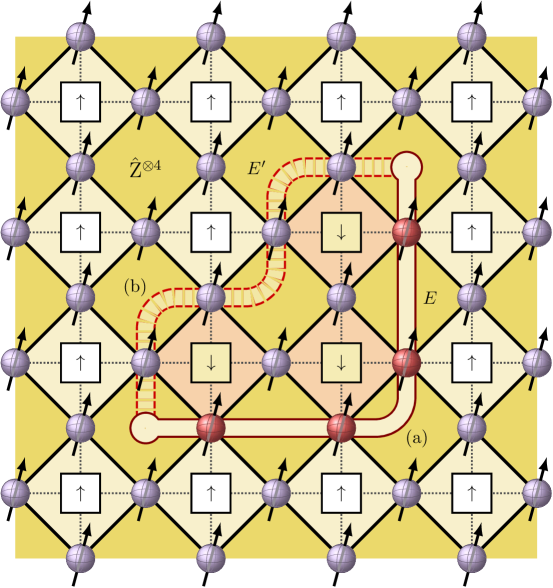
Figure 1: For the toric code, qubits are arranged on a square lattice, with stabilizer operators acting on plaquettes of four qubits. The figure shows the spin placement to sample chains from an error class $\bar{E}$: (a) A reference error chain $E$ defines the error class; the interactions are anti-ferromagnetic along this chain. (b) A chain which differs from the reference chain by a product of spin-plaquettes: Together with the reference chain it forms the boundary $E+E^{\prime}$ of a flipped domain of spins. The terms along $E^{\prime}$ are excited, while the ones along $E$ are now satisfied. Thus the Boltzmann weight for this configuration is proportional to $(p/(1-p))^{|E^{\prime}|-|E^{\prime}|}$.

For a constant qubit error rate $p$, the probability $\mathcal{P}$ for a specific error chain $E$ is determined by the number of faulty qubits $\left|E\right|$:

$$\mathcal{P}(E)=(1-p)^{N-\left|E\right|}(p)^{\left|E\right|}\,,$$ (1)

where $N$ is the number of qubits in the setup. Equivalently, we can describe this error chain with Boolean values $n_{\ell}^{E}\in\{0,1\}$ for each qubit $\ell$, describing whether an error occurred. The probability in (1) can then be written as

$$\mathcal{P}(E)=\prod_{\ell}\,(1-p)^{N-n_{\ell}^{E}}(p)^{n_{\ell}^{E}}=(1-p)^{N}\prod_{\ell}\,\left(\frac{p}{1-p}\right)^{n_{\ell}^{E}}\,,$$ (2)

where the product is over all qubits $\ell$. Because the stabilizer measurements only yield the boundary of the error chain, there are many other error chains $E^{\prime}$ that are compatible with the same error syndrome. If two chains $E$ and $E^{\prime}$ share the same boundary, then they can only differ by a set of cycles $C$, which have no boundary. The relative probability of $E^{\prime}=E+C$, compared to $E$, depends on the relative number of faulty qubits, which increases for every qubit in $C\setminus E$ but decreases for qubits in $C\cap E$. Therefore, using analogous Boolean descriptors for the chain, $n_{\ell}^{C}$, we can write the relative probability $\mathcal{P}(E^{\prime})/\mathcal{P}(E)$ as:

$$\frac{\mathcal{P}(E^{\prime})}{\mathcal{P}(E)}=\prod_{\ell}\left(\frac{p}{1-p}\right)^{n_{\ell}^{C}(1-2n_{\ell}^{E})}\propto\prod_{\ell}\exp[\beta J\tau_{\ell}(\underbrace{1-2n_{\ell}^{C}}_{u_{\ell}})]\,.$$ (3)

The newly-defined variable $u_{\ell}\in\{\pm 1\}$ is negative for all links in $C$ and we have introduced carefully-chosen coupling constants $\tau_{\ell}\in\{\pm 1\}$ and a factor $\beta J$ such that

$$e^{-2\beta J\tau_{\ell}}=[p/(1-p)]^{1-2n_{\ell}^{E}}\,.$$ (4)

Note that the sign of $\tau_{\ell}$ is dictated by the presence of an error in the reference chain $E$, and $J$ is related to the error probability via the Nishimori condition [30]:

$$-2\beta J=\ln\left(\frac{p}{1-p}\right)\,.$$ (5)

The constraint for $C$ to be cyclic (no boundary) imposes the additional requirement that the number of adjacent faulty qubits $\ell\in C$ must be even for every plaquette. One way to satisfy this condition is to introduce Ising variables $s_{i}\in\{\pm 1\}$ for each plaquette of the opposite colour. That is, each spin represents an elementary cycle around a plaquette and larger cycles are formed by combining several of these elementary loops. For any choice of the spin variables $s_{i}$, the variables $u_{\ell}=s_{i}s_{j}$, with $\ell$ the edge between plaquettes $i$ and $j$, describes such a cyclic set $C$ (see figure 1).

We have therefore found that the spin configurations enumerate all error chains $E^{\prime}$ that differ from the reference chain $E$ by a tileable set of cycles. With the Nishimori relation (5) their Boltzmann weight is also proportional to the probability of the respective error chain. Therefore, it is possible to sample the fluctuations of error chains within the same error class by sampling configuration from the classical statistical model described by the partition function

$$\mathcal{Z}_{\{\tau_{ij}\}}=\sum_{\{s\}}\exp\big{(}-\beta J\sum_{\left\langle{i,j}\right\rangle}\tau_{ij}s_{i}s_{j}\big{)}\,.$$ (6)

Here $J$ is dictated by the Nishimori condition (5) and $\tau_{ij}$ are quenched, disordered interactions which are negative if the associated qubit is faulty in the reference chain. Because the mapping identifies error chains with domain walls and their difference with a flipped patch of spins, we can identify the ordered state with the scenario where error chain fluctuations are small and correct error classification is feasible. And while this sampling does not implicitly consider homologically nontrivial cycles, we can interpret percolating domain walls as error fluctuations which are too strong to reliably distinguish cycles of different homology.

Because $\beta J$ and $p$ can only be related on the Nishimori line for the mapping between the quantum problem and the statistical-mechanical counterpart to work, we need to compute the point in the disorder $p$ and critical temperature $T_{{\mathrm{\scriptscriptstyle{c}}}}(p)$ plane where the Nishimori line (5) intersects the phase boundary between a paramagnetic and a ferromagnetic phase, see figure 3. This point, $p_{{\mathrm{\scriptscriptstyle{c}}}}$ then corresponds to the error threshold of the underlying topologically-protected quantum computing proposal. For the case of the toric code with qubit flip errors, the problem maps onto a two-dimensional random-bond Ising model described by the Hamiltonian:

$$\mathcal{H}=-J\sum_{\langle i,j\rangle}\tau_{ij}s_{i}s_{j}\,,$$ (7)

where $J$ is a global coupling constant chosen according to the Nishimori condition (5), $s_{i}\in\{\pm 1\}$, the sum is over nearest neighbor pairs, and the mapping requires $\tau_{ij}$ to be quenched bimodal random interactions, distributed according to the error rate $p$:

$$\mathcal{P}(\tau_{ij})=\left\{\begin{array}[]{cl}+1\;;&1-p\\ -1\;;&p\,.\end{array}\right.$$ (8)

For the toric code with qubit flip errors $p_{{\mathrm{\scriptscriptstyle{c}}}}\approx 10.9$% [31, 32, 25, 33], i.e., as long as the fraction of faulty physical qubits does not exceed $10.9$%, errors can be corrected. In the next section we outline the procedure used to estimate different error thresholds using Monte Carlo methods.

3 Estimating error thresholds using Monte Carlo methods

The partition function found in the mapping for Kitaev’s toric code can be interpreted as a classical spin model where the different spin configurations are weighted proportional to the likelihood of the error chain they represent. The existence of such a relationship is instrumental in understanding the fluctuations of error chains, because it allows for the computation of the thermodynamic value of the error threshold using tools and methods from the study of statistical physics of disordered systems.

3.1 Algorithms

The simulations are done using the parallel tempering Monte Carlo method [34, 35, 36, 37, 38]. The method has proven to be a versatile “workhorse” in many fields [39]. Similar to replica Monte Carlo [34], simulated tempering [40], or extended ensemble methods [41], the algorithm aims to overcome free-energy barriers in the free energy landscape by simulating several copies of a given Hamiltonian at different temperatures. The system can thus escape metastable states when wandering to higher temperatures and relax to lower temperatures again in time scales several orders of magnitude smaller than for a simple Monte Carlo simulation at one fixed temperature. A delicate choosing of the individual temperatures is key to ensure that the method works efficiently. See, for example, [38].

The classical Hamiltonians obtained when computing error thresholds in topological quantum computing proposals all have quenched bond disorder, i.e., a complex energy landscape with many metastable states. As such, parallel tempering is the algorithm of choice when simulating these systems, especially when temperatures are low and disorder high (for example, close to the error threshold) where thermalization is difficult.

Equilibration is typically tested in the following way: We study how the results for different observables vary when the simulation time is successively increased by factors of 2 (logarithmic binning). We require that the last three results for all observables agree within error bars.

3.2 Determination of the phase boundary

To determine the error threshold we have to first determine the phase boundary between an ordered and disordered phase. In most cases this phase boundary can be determined by studying dimensionless functions of local order parameters like the magnetization. Note, however, that some models map onto lattice gauge theories where averages of all local order parameters are zero. In these specific cases we use other approaches outlined below.

As an example, for the case of the toric code, we study a transition between a paramagnetic and a ferromagnetic phase. The transition is determined by a finite-size scaling of the dimensionless two-point finite-size correlation length divided by the system size [42, 43, 44, 45]. We start by determining the wave-vector-dependent susceptibility

$$\chi(k)=\frac{1}{N}\sum_{ij}^{N}\langle S_{i}S_{j}\rangle_{T}\;e^{i{\bf k}\cdot({\bf R}_{i}-{\bf R}_{j})}\;.$$ (9)

Here, $\langle\cdots\rangle_{T}$ represents a thermal (Monte Carlo time) average and ${\bf R}_{i}$ is the spatial location of the $N$ spins. The correlation length is then given by

$$\xi_{L}=\frac{1}{2\sin(k_{\rm min}/2)}\sqrt{\frac{[\chi(k=0)]_{\rm av}}{[\chi(k_{\rm min})]_{\rm av}}-1},$$ (10)

where $k_{\rm min}=(2\pi/L,0)$ is the smallest nonzero wave vector and $[\cdots]_{\rm av}$ represents an average over the different error configurations (bond disorder). The finite-size correlation length divided by the system size has the following simple finite-size scaling form:

$$\xi_{L}/L\sim\widetilde{X}(L^{1/\nu}[T-T_{{\mathrm{\scriptscriptstyle{c}}}}]),$$ (11)

where $\nu$ is a critical exponent and $T_{{\mathrm{\scriptscriptstyle{c}}}}$ represents the transition temperature we need to construct the phase boundary. Numerically, finite systems of linear size $L$ are studied. In that case the function $\xi_{L}/L$ is independent of $L$ whenever $T=T_{{\mathrm{\scriptscriptstyle{c}}}}$ because then the argument of the function $\tilde{X}$ is zero. In other words, if a transition is present, the data cross at one point (up to corrections to scaling). This is illustrated in figure 2 for the case of the toric code and $4$% faulty qubits: Data for different system sizes cross at $T_{{\mathrm{\scriptscriptstyle{c}}}}\approx 1.960(2)$ signaling a transition. Because finite-size scaling corrections are typically small, one can use the estimate of $T_{{\mathrm{\scriptscriptstyle{c}}}}$ obtained as a very good approximation to the thermodynamic limit value.

The simulations must now be repeated for different fractions $p$ of faulty qubits, i.e., for different fractions of ferromagnetic-to-antiferromagnetic bonds between the classical Ising spins. This then allows one to build a temperature–disorder phase diagram as shown in figure 3 for the case of the toric code. The error threshold then corresponds to the point where the Nishimori line (dashed line in figure 3) intersects the phase boundary (solid line in figure 3). In this particular case this occurs for $p_{{\mathrm{\scriptscriptstyle{c}}}}\approx 10.9$%, i.e., as long as there are less than $10.9$% physical qubit flips, errors can be corrected in the quantum code.

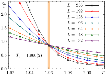
Figure 2: Two-point finite-size correlation length $\xi_{L}/L$ as a function of temperature for different system sizes $L$ for the two-dimensional random-bond Ising model with a fraction of $p=0.04$ antiferromagnetic bonds. This corresponds to a toric code with $4$% faulty qubits (bit flip errors). The data cross at $T_{{\mathrm{\scriptscriptstyle{c}}}}\approx 1.960(2)$, signaling a transition (shaded area; the width represents the statistical error bar). The data cross cleanly and show only small finite-size corrections (these become stronger close to $p_{{\mathrm{\scriptscriptstyle{c}}}}$).

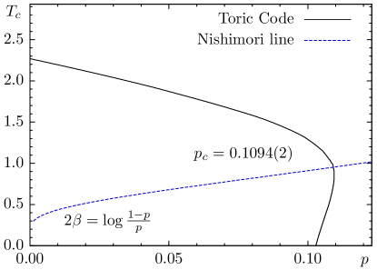
Figure 3: Phase diagram for the two-dimensional random-bond Ising model. $p$ represents the fraction of antiferromagnetic bonds (fraction of flipped qubits) and $T_{{\mathrm{\scriptscriptstyle{c}}}}$ the transition temperature. The dashed line is the Nishimori line. The point where it intersects the phase boundary (solid line) represents the error threshold which, in this case, is $p_{{\mathrm{\scriptscriptstyle{c}}}}\approx 0.1094(2)$ [31, 46, 32, 25, 33]. This means that errors can be corrected as long as no more than $10.9$% physical qubits have flipped. Phase boundary data taken from [47].

4 Results

We now summarize our results for different topological codes, as well as different sources of error. Note that the mappings onto the statistical-mechanical models are often complex and, for the sake of brevity, we refer the reader to the individual manuscripts cited.

4.1 Toric code with qubit-flip errors

The toric code with qubit-flip errors has already been described in detail in section 2. As stated before, the error-correction process maps onto a two-dimensional random-bond Ising model:

$$\mathcal{H}=-J\sum_{i,j}\tau_{\langle ij\rangle}s_{i}s_{j}\,,\;\;\;\;\;\;\;\;\;\;\;\;\;\;\mathcal{P}(\tau_{ij})=\left\{\begin{array}[]{cl}+1\;;&1-p\\ -1\;;&p\end{array}\right.$$ (12)

where $J$ is a global coupling constant chosen according to the Nishimori condition (5), $s_{i}\in\{\pm 1\}$, and the sum is over nearest neighbors. The error threshold for the toric code was computed by Dennis et al. in [4], $p_{{\mathrm{\scriptscriptstyle{c}}}}=0.1094(2)$, with a lower bound given by Wang et al. in [46] (the phase diagram is reentrant [46, 33, 47]). Note that more detailed estimates of $p_{{\mathrm{\scriptscriptstyle{c}}}}$ followed later [31, 32, 25, 33]. The associated phase boundary is shown in figure 3.

4.2 Colour codes with qubit-flip errors

In 2006 Bombín and Martín-Delgado showed that the concept of topologically-protected quantum bits could also be realized on trivalent lattices with three-colourable faces. The topological colour codes they introduced [6] share similar properties to the toric code: stabilizer generators are intrinsically local and the encoding is in a topologically-protected code subspace. However, colour codes are able to encode more qubits than the toric code and, for some specific lattice structures, even gain additional computational capabilities.

In colour codes, qubits are arranged on a trivalent lattice (hexagonal or square octagonal), such that each qubit contributes a term of the form $\beta J\tau_{ijk}s_{i}s_{j}s_{k}$ in the mapping. In the case of hexagonal lattices, the partition function takes the form [18]

$$\mathcal{Z}_{\{\tau_{ijk}\}}=\sum_{\{s\}}\exp\big{(}-\beta J\!\!\!\!\sum_{i,j,k\in\{\triangle\}}\!\!\!\tau_{ijk}s_{i}s_{j}s_{k}\big{)}\,.$$ (13)

Equation (13) describes a disordered statistical system with three-spin interaction for each plaquette. Note that the spins $s_{i}$ defined for the mapping are located on the triangular lattice which is dual to the original hexagonal arrangement. Every qubit corresponds to a triangle in the new lattice and dictates the sign of the associated plaquette interaction via $\tau_{ijk}$. Thus, the statistical-mechanical Hamiltonian for the system related to colour codes [as described by (13)] is given by

$$\mathcal{H}=-J\!\!\!\sum_{i,j,k\in\{\triangle\}}\!\!\tau_{ijk}s_{i}s_{j}s_{k}\,,$$ (14)

where $J$ is a global coupling constant chosen according to the Nishimori condition, $s_{i}\in\{\pm 1\}$, and the mapping requires $\tau_{ijk}$ to satisfy

$$\mathcal{P}(\tau_{ijk})=\left\{\begin{array}[]{cl}+1\;;&1-p\\ -1\;;&p\end{array}\right.\,.$$ (15)

Note that the disordered three-body Ising model on the triangular lattice with $p=0.5$ is NP-hard and therefore numerically difficult to study [48]. We would like to emphasize that colour codes on square-octagonal lattices are of particular interest, because, contrary to both toric codes and colour codes on honeycomb lattices, they allow for the transversal implementation of the whole Clifford group of quantum gates.

Figure 4 shows the $p$–$T_{{\mathrm{\scriptscriptstyle{c}}}}$ phase diagram for colour codes on hexagonal (maps onto a triangular lattice; empty circles), as well as square octagonal lattices (maps onto a Union Jack lattice; empty triangles). In addition, the solid (black) line is the phase boundary for the toric code. Surprisingly, the phase boundaries for all three models agree within statistical error bars, suggesting that colour as well as toric codes share similar error thresholds $p_{{\mathrm{\scriptscriptstyle{c}}}}$. This is surprising, because the underlying statistical models have very different symmetries and are in different universality classes. For example, in the absence of randomness, the three-body Ising model on a triangular lattice is in a different universality class than the two-dimensional Ising model. Whereas for three-body Ising model on a two-dimensional triangular lattice $\nu=\alpha=2/3$ [49], for the two-dimensional Ising model $\nu=1$ and $\alpha=0$. The disordered three-body Ising model on a triangular lattice has not been studied before, therefore highlighting again the fruitful relationship between quantum information theory and statistical physics.

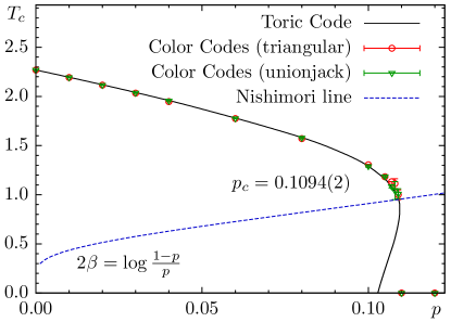
Figure 4: Comparison of the $p\,$–$\,T_{c}$ phase diagram for the toric code (solid black line) and the results for random three-body Ising model on a triangular lattice (red), as well as on a Union Jack lattice (green). The error threshold is indicated by the intersection of the phase boundary with the Nishimori line (dashed blue) For $p>p_{c}\approx 0.109$ the ferromagnetic order is lost. Note the agreement with the toric code. Data taken from Refs. [18], [50], and [47].

Finally, our results also show that the enhanced computing capabilities of colour codes on the square-octagonal lattice do not come at the expense of an increased susceptibility to noise.

4.3 Depolarizing channel

The effects of single-qubit operations can be decomposed into qubit flips and phase flips, as well as a combination thereof; represented by the three Pauli matrices $\hat{\mathrm{X}}$, $\hat{\mathrm{Z}}$, and $\hat{\mathrm{Y}}$. When describing decoherence effects as a noisy channel, depolarizing noise is characterized by equal probability for each type of error to occur, i.e., $p_{x}=p_{y}=p_{z}\vcentcolon=p/3$. Note that the depolarizing channel is more general than the bit-flip channel, because it allows for the unified, correlated effect of all three basic types of errors [8, 23].

As in the previous mappings, in order to express the probability of an error class in terms of a classical Boltzmann weight, we need to associate with each elementary error loop a classical Ising spin. However, because of the error correlations, we cannot treat errors of different types independently any more. Instead, the resulting model contains spins of different types, according to the types of stabilizers used in the code. In fact, the mapping can be carried out in a very general way that requires no assumptions on the individual error rates or the actual quantum setup, see [23]. However, here we merely provide a brief explanation of the resulting Hamiltonian for the Toric code within the depolarizing channel.

In addition to the stabilizers of type $\hat{\mathrm{Z}}^{\otimes 4}$ (see section 2), the toric code also places stabilizers of type $\hat{\mathrm{X}}^{\otimes 4}$ on the remaining squares in the checkerboard decomposition. These allow for the concurrent detection of possible phase errors on the physical qubits. As a result, whenever a qubit flips, this is signaled by adjacent $\hat{\mathrm{Z}}$-stabilizers, whereas a qubit attaining a phase error is identified by $\hat{\mathrm{X}}$-stabilizers. Additionally, a combined qubit flip and phase error affects both the neighboring $\hat{\mathrm{Z}}$ and $\hat{\mathrm{X}}$-stabilizers. Therefore, the resulting Hamiltonian contains three terms per qubit; one describing each of the aforementioned scenarios:

$$\mathcal{H}=-J\sum_{ijk\ell}(\tau_{ij}^{x}s_{i}^{z}s_{j}^{z}+\tau_{k\ell}^{z}s_{k}^{x}s_{\ell}^{x}+\tau_{ijk\ell}^{y}s_{i}^{z}s_{j}^{z}s_{k}^{x}s_{\ell}^{x})\,,$$ (16)

where the sum is over all qubits, the indices $i$, $j$, $k$ and $\ell$ denote the four affected elementary equivalences and the sign of $\tau^{w}$ is dictated by whether the qubit has suffered an error of type $w\in\{x,y,x\}$. This Hamiltonian describes a classical Ising model that can be interpreted as two stacked square lattices which are shifted by half a lattice spacing, see figure 6. In addition to the standard two-body interactions for the top and bottom layers, the Hamiltonian also includes four-body terms (light green in the figure) that introduce correlations between the layers. Interestingly, toric codes under the depolarizing channel are related to the eight-vertex model introduced by Sutherland [51], as well as Fan and Wu [52], and later solved by Baxter [53, 54, 55].

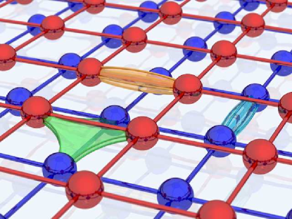
Figure 5: When computing the stability of the toric code to depolarization, the problem maps onto a classical statistical Ising model on two stacked square lattices with both two-body and four-body interactions.

Figure 6: For colour codes, the spins are arranged on triangular lattices. In addition to the three-body interactions found for qubit-flip errors, both layers are connected via six-body interactions (light green).

For topological colour codes, qubits are arranged on trivalent lattices (hexagonal or square-octagonal) and the problem then maps onto either a triangular or Union Jack lattice (see section 4.2). For the depolarizing channel, an analogous mapping to the previous one relates this quantum setup to a Hamiltonian of the form:

$$\mathcal{H}=-J\sum_{ijk}(\tau_{ijk}^{x}s_{i}^{z}s_{j}^{z}s_{k}^{z}+\tau_{ijk}^{z}s_{i}^{x}s_{j}^{x}s_{k}^{x}+\tau_{ijk}^{y}s_{i}^{z}s_{j}^{z}s_{k}^{z}s_{i}^{x}s_{j}^{x}s_{k}^{x})\,.$$ (17)

The details of this mapping are also contained in [23]. In addition to the in-plane three-body plaquette interactions that appear already when studying individual qubit-flips (see section 4.2), here additional six-body interactions add the necessary correlations between the planes (see figure 6). The resulting model maps to an eight-vertex model on a Kagomé lattice [56].

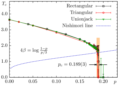
Figure 7: Estimated phase boundary for the models related to the depolarizing channel. The individual data sets represent the toric code (black), as well as colour codes on triangular (red) and Union Jack (green) lattices. The error threshold $p_{{\mathrm{\scriptscriptstyle{c}}}}=0.189(3)$ corresponds to the point where the Nishimori line (dashed, blue) intersects the phase boundary. Remarkably, the phase boundaries for all three codes agree within error bars. Data taken from [23].

We perform simulations using the sublattice magnetization [23] to compute the susceptibility, and construct again the $p\,$–$\,T_{{\mathrm{\scriptscriptstyle{c}}}}$ phase diagram for the toric code, as well as colour codes on both hexagonal and square-octagonal lattices. Note also, that the Nishimori condition changes slightly in this particular context (see the equation in figure 7 and [23]). Interestingly, the phase boundaries for all three error-correction models agree and we estimate conservatively an error threshold of $p_{{\mathrm{\scriptscriptstyle{c}}}}=0.189(3)$ for all three models. A similar study based on duality considerations [23, 24] yields results that agree within error bars. It is remarkable that the error threshold to depolarization errors for different classes of topological codes studied is larger than the threshold for expected uncorrelated errors, $p_{{\mathrm{\scriptscriptstyle{c}}}}^{\prime}=(3/2)p_{c,{\mathrm{\scriptscriptstyle{flip}}}}\approx 16.4\%$. This is encouraging and shows that topological codes are more resilient to depolarization than previously thought. It also suggests that a detailed knowledge of the correlations in the error source can allow for a more efficient, custom-tailored code to be designed.

4.4 Subsystem Codes

All topological codes share the advantage that the quantum operators involved in the error-correction procedure are local, thus rendering actual physical realizations more feasible. However, in practice the decoherence of quantum states is not the only source of errors: Both syndrome measurement and qubit manipulations are delicate tasks and should be kept as simple as possible to minimize errors. For the toric code and topological colour codes, the check operators, while local, still involve the combined measurement of $4$, $6$, or even $8$ qubits at a time.

By using concepts from subsystem stabilizer codes, Bombin was able to introduce a class of topological subsystem codes [8] that only requires pairs of neighboring qubits to be measured for syndrome retrieval. This is achieved by designating some of the logical qubits as “gauge qubits” where no information is stored. Due to the resulting simplicity of the error-correction procedure, these are very promising candidates for physical implementations.

The generation and mapping of a quantum setup that incorporates all these desired concepts is rather involved; we refer the reader to the relevant papers in Refs. [8] and [57]. One possible arrangement is shown in figure 8, consisting of qubits arranged in triangles, squares and hexagons with stabilizer operators of different types connecting neighboring pairs. In the mapping to a classical system, the setup then corresponds to a set of Ising spins (one for each stabilizer) with interactions dictated by how each stabilizer is affected by errors on adjacent qubits. This gives rise to a Hamiltonian of the general form

$$\mathcal{H}=-J\sum_{\ell}\sum_{w=x,y,z}\tau_{\ell}^{w}\prod_{i}s_{i}^{g_{i\ell}^{w}}\,,$$ (18)

where $\ell$ enumerates all qubit sites, $w$ the three error types and $i$ iterates over all Ising spins, respectively. The exponent $g_{i\ell}^{w}\in\{0,1\}$ determines whether the stabilizer $i$ is affected by an error of type $w$ on qubit $\ell$. Thus, for every qubit $\ell$ and error type $w$, the Hamiltonian contains a term of the form $-J\tau_{\ell}^{w}s_{i}s_{j}s_{k}$, where $J$ is a constant, $\tau_{\ell}^{w}$ is a quenched random variable (representing a possible qubit error) and the product contains all Ising spins corresponding to stabilizers affected by such an error.

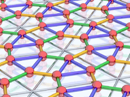
Figure 8: Topological subsystem codes combine aspects of both topological error-correction codes and subsystem codes. Starting from a triangular lattice, the construction places three qubits in each triangle with stabilizers acting on pairs of them. Here the red spheres represent individual qubits, interconnected with stabilizers of type $\hat{\mathrm{X}}$ (yellow), $\hat{\mathrm{Y}}$ (green) and $\hat{\mathrm{Z}}$ (blue). The original triangular lattice for the construction is shown in grey. Despite only relying on two-qubit stabilizers, this setup is able to preserve quantum information up to a threshold of $5.5$%.

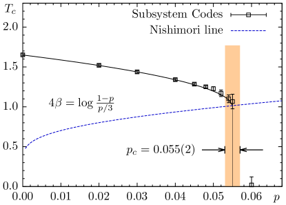
Figure 9: Disorder–temperature phase diagram for subsystem codes under depolarizing noise. The error threshold is given by the intersection of the phase boundary (solid line) with the Nishimori line (dashed). Our (conservative) numerical estimate is $p_{{\mathrm{\scriptscriptstyle{c}}}}=0.055(2)$ (orange vertical bar). Despite the low threshold compared to other proposals, this code is very promising due to the simpler stabilizers involved in the error-correction process.

Using Monte Carlo simulations, we compute the temperature–disorder phase diagram for the aforementioned statistical-mechanical model (see figure 9) and estimate an error threshold of $p_{{\mathrm{\scriptscriptstyle{c}}}}=0.055(2)$ [57], which is remarkable given the simplicity of the error-correction procedure. Note that this critical error rate is (numerically) smaller than the threshold calculated for the toric code, as well as topological colour codes. This is a consequence of a compromise for a much simpler syndrome-measurement and error-correction procedure: with a streamlined syndrome measurement process, the physical qubits are given less time to decohere and the error rate between rounds of error correction in an actual physical realization will be smaller.

4.5 Topological codes with measurement errors

So far we have only considered different types of errors that might occur on the physical qubits (at a rate $p$), while the process of syndrome measurement was assumed to be flawless. However, if additional measurement errors occur (at a rate $q$), we need to devise a scheme that can preserve quantum information over time even if intermediate measurements are faulty. This leads to the notion of so-called “fault-tolerant” codes: in this case, our best option is actually to continuously measure and correct errors as they are detected. Note that this introduces errors whenever the syndrome is faulty and these pseudo errors can only be detected and corrected in a later round of error correction.

This process of alternating measurement and correction phases can be modeled by considering vertically stacked copies of the original quantum setup, each representing one round of error correction. In this simplified scenario, errors only occur at discrete time steps, and it is instructive to think of the additional vertical dimension as a time. In particular, the measurements are represented by vertical connections between the plaquettes where the corresponding stabilizer resides. Then, the state of each layer is related to the layer immediately before it by the effect of the error channel, followed by one round of syndrome measurement and error correction. For no measurement errors (i.e., $q=0$) all errors are detected perfectly and are corrected within one step. Consequently, there is no inter-relation between the errors found in consecutive layers. If $q>0$, however, some errors can remain and new ones might be introduced due to the faulty syndrome measured. In analogy to the error chains seen earlier, we refer to these errors persevering over time as “error histories.”

Figure 10: Toric code with measurement errors. (a) Elementary loops are error chains as seen before (figure 1). (b) Vertical links represent stabilizer measurements. This minimal error history consists of two consecutive qubit flips that remain unnoticed due to faulty measurements. (c) A more complex error history.

Mapping the qubit-flip and measurement problem in the toric code to a statistical-mechanical Ising model to compute the error threshold [4, 46, 58] yields a Hamiltonian of them form

$$\mathcal{H}=-J\sum_{\square}\tau_{\square}^{{\mathrm{\scriptscriptstyle{s}}}}s^{{\mathrm{\scriptscriptstyle{s}}}}_{i}s^{{\mathrm{\scriptscriptstyle{s}}}}_{j}s^{{\mathrm{\scriptscriptstyle{t}}}}_{k}s^{{\mathrm{\scriptscriptstyle{t}}}}_{\ell}-K\sum_{\square}\tau_{\square}^{{\mathrm{\scriptscriptstyle{t}}}}s^{{\mathrm{\scriptscriptstyle{t}}}}_{i}s^{{\mathrm{\scriptscriptstyle{t}}}}_{j}s^{{\mathrm{\scriptscriptstyle{t}}}}_{k}s^{{\mathrm{\scriptscriptstyle{t}}}}_{\ell}\,,$$ (19)

where the first [second] sum is over all qubits [vertical links] in the lattice. Furthermore, we have introduced positive interaction constants $J$ and $K$ to be chosen according to the (adapted) Nishimori conditions [30] $\exp(-2\beta J)=p/(1-p)$ and $\exp(-2\beta K)=q/(1-q)$. Note that each of the spatial spins $s^{{\mathrm{\scriptscriptstyle{s}}}}$ represents an in-plane (i.e., horizontal) elementary loop that consists purely of qubit flip errors, while the time-like spins $s^{{\mathrm{\scriptscriptstyle{t}}}}$ represent minimal error histories (vertical loops) that consist of two qubit flip errors and two faulty measurements (see figure 10). As for the toric code without measurement errors, these loops are used to tile the difference between two error chains. Thus different spin configurations represent error chains of the same class (sharing the same end points), albeit with different qubit and measurement errors. And, given the Nishimori condition, the Hamiltonian ensures that the Boltzmann weight corresponds to the relative probability of each scenario.

Equation (19) describes a disordered Ising lattice gauge theory with multi-spin interactions and four parameters, $\beta J$, $\beta K$, $p$ and $q$. The mapping is valid along the two-dimensional Nishimori sheet. We have treated spatial and time-like equivalences separately to allow for different qubit and measurement error rates. Interestingly, for the special case $p=q$, the resulting Hamiltonian is isotropic, i.e.,

$$\mathcal{H}=\sum_{\square}\tau_{{\scriptscriptstyle{\square}}}s_{i}s_{j}s_{k}s_{l}\,,$$ (20)

where $\square$ represents a sum over all plaquettes in the lattice (both vertical and horizontal). Because $p=q$ also implies $J=K$ via the Nishimori condition, the model to investigate for this special case has only two parameters, namely $\beta J$ and $p$.

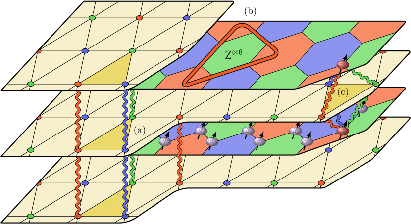
Figure 11: Lattice structure for colour codes that consists of stacked triangular and hexagonal layers. (a) Vertical connections represent the measurement history, while the qubits reside on hexagonal lattice sites. The lattice gauge theory has two elementary equivalences: (b) Coloured loops in the hexagonal planes. (c) Temporal equivalences consisting of two consecutive qubit errors and three faulty measurements.

The model is a ${\mathbb{Z}}_{2}$ lattice gauge theory [46, 58], so we cannot use a local order parameter to determine the phase transition in our numerical simulations. Instead we consider the peak in the specific heat and the distribution of Wilson loop values to identify ordering in the system [59]. The latter observable is interesting because the first-order transition present in this system causes a double-peak structure near the transition. Even though the effect is smeared out when disorder is introduced, we can still reliably detect this shift of weight from one peak to the other by performing a finite-size scaling analysis of the skewness (third-order moment of the distribution). The temperature where the skewness is zero represents the point where the distribution of Wilson loops is double-peaked and symmetric, i.e., the phase transition. Comparisons to more traditional methods, such as a Maxwell construction, show perfect agreement. Note that this approach is generic and can be applied to any Hamiltonian that has a first-order transition.

An analogous mapping and analysis is also possible for topological colour codes with measurement errors. In this case, one considers a three-dimensional lattice consisting of stacked triangular layers, each representing one round of error syndrome measurement. The qubits reside on intermediate hexagonal layers and are connected to their respective check operators via vertical links as indicated in figure 11. In this case, the mapping to compute the error threshold for faulty measurements and qubit flips produces a ${\mathbb{Z}}_{2}\times{\mathbb{Z}}_{2}$ lattice gauge theory given by the Hamiltonian

$$\mathcal{H}=-J\sum_{\triangle}\tau_{\triangle}s^{{\mathrm{\scriptscriptstyle{s}}}}_{i}s^{{\mathrm{\scriptscriptstyle{s}}}}_{j}s^{{\mathrm{\scriptscriptstyle{s}}}}_{k}s^{{\mathrm{\scriptscriptstyle{t}}}}_{l}s^{{\mathrm{\scriptscriptstyle{t}}}}_{m}-K\sum_{{\mbox{\tiny\hexagon}}}\tau{{\mbox{\tiny\hexagon}}}s^{{\mathrm{\scriptscriptstyle{t}}}}_{i}s^{{\mathrm{\scriptscriptstyle{t}}}}_{j}s^{{\mathrm{\scriptscriptstyle{t}}}}_{k}s^{{\mathrm{\scriptscriptstyle{t}}}}_{l}s^{{\mathrm{\scriptscriptstyle{t}}}}_{m}s^{{\mathrm{\scriptscriptstyle{t}}}}_{n}\,,$$ (21)

where the first [second] sum is, again, over all qubits [measurements], represented by the product of the five [six] equivalences affected by the corresponding errors. The choice of the constants $J$ and $K$ is done as for the toric code following the modified Nishimori conditions. This Hamiltonian also describes an Ising lattice gauge theory, but even for the choice of $p=q$ it is not isotropic as was the case for the toric code with measurement errors.

Both models for topological codes with measurement errors are studied numerically using Monte Carlo simulations [59]. Interestingly, the thresholds calculated for the toric code and topological colour codes do not agree when possible measurement errors are taken into account. While the toric code can only correct up to $3.3\%$ errors when $p=q$, colour codes remain stable up to $4.8\%$. This remarkable discrepancy is also seen in numerical studies where we allow $p$ and $q$ to be different (as long as $q>0$), see figure 12.

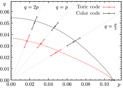
Figure 12: Preliminary results: Error threshold for bit flip errors (probability $p$) with different probabilities of measurement errors $q$ for the toric code (red) and colour codes (black). For perfect error syndrome measurement, i.e., $q=0$ (horizontal axis), the error thresholds of both codes agree, [$p_{{\mathrm{\scriptscriptstyle{c}}}}=0.109(2)$]. However, for a non-vanishing measurement error rate ($q>0$), the error thresholds differ. The dashed lines are guides to the eye. Numerical values listed in Table 1.

5 Summary and conclusions

In Table 1 we summarize our results for different combinations of topological codes and error sources. As can be seen, the different proposals for topologically-protected quantum computation are very resilient to the different error sources.

Note that the results for different error channels in Table 1 cannot be compared directly: For the qubit-flip channel, $p_{{\mathrm{\scriptscriptstyle{c}}}}$ only refers to the maximum amount of flip errors that can be sustained, while for the depolarizing channel $p_{{\mathrm{\scriptscriptstyle{c}}}}$ is the sum of all three basic error types. Furthermore, the lower threshold for subsystem codes is the result of a compromise for a simpler error-correction procedure. Likewise, a lower value of $p_{{\mathrm{\scriptscriptstyle{c}}}}$ is to be expected in fault-tolerant schemes due to the additional presence of measurement errors. Remarkably, the error stability of the toric code and topological colour codes appears to be different only in the fault-tolerant regime where the mapping to a statistical-mechanical model produces a lattice gauge theory, despite finding perfect agreement in all other error channels.

We have outlined the mapping and subsequent analysis of several topological error-correction codes to classical statistical-mechanical Ising spin models with disorder. Because error chains correspond to domain walls under this mapping, an ordered state in the classical model can be identified with the scenario of feasible error correction, while the proliferation of errors in the quantum setup is associated with a disordered state in the classical model. After numerically calculating the disorder–temperature phase diagram of the (classical) statistical spin models, the error threshold can be identified with the intersection point of the phase boundary with the Nishimori line. This critical error threshold represents the maximum amount of perturbation each setup can sustain and does not include the effects of realistic device implementations. However, the fact that these “theoretical” best-case thresholds are so high is rather promising.

We conclude by highlighting again the beautiful synergy between quantum error correction and novel disordered spin models in statistical physics. We hope that these results will encourage scientists specialized in analytical studies of disordered systems to tackle these simple yet sophisticated Hamiltonians.

Error Source	Topological Error Code	Threshold $p_{{\mathrm{\scriptscriptstyle{c}}}}$
Qubit-Flip	Toric code	$0.109(2)$
Qubit-Flip	Colour code (honeycomb lattice)	$0.109(2)$
Qubit-Flip	Colour code (square-octagonal lattice)	$0.109(2)$
Depolarization	Toric code	$0.189(2)$
Depolarization	Colour code (honeycomb lattice)	$0.189(2)$
Depolarization	Subsystem code	$0.055(2)$
Qubit-Flip & Measurement	Toric code	$0.033(5)$
Qubit-Flip & Measurement	Toric code ($q=2p$)	$0.017(3)$
Qubit-Flip & Measurement	Toric code ($q=p/2$)	$0.047(6)$
Qubit-Flip & Measurement	Colour code ($p=q$)	$0.048(3)$
Qubit-Flip & Measurement	Colour code ($q=2p$)	$0.025(4)$
Qubit-Flip & Measurement	Colour code ($q=p/2$)	$0.066(7)$

Table 1: Summary of error thresholds calculated numerically. Note that our estimate for the toric code with qubit-flip and measurement errors agrees with the results of Wang et al. [46] and Ohno et al. [58]. The most precise estimate for the toric code with qubit-flip errors is $p_{{\mathrm{\scriptscriptstyle{c}}}}=0.10919(7)$, see [33].

Part of the figures shown in this work are from the PhD Thesis of Ruben S. Andrist (Eidgenössische Technische Hochschule Diss. No. 20588). Work done in collaboration with H. Bombin (Perimeter Institute), M. A. Martin-Delgado (Universidad Complutense de Madrid), and C. K. Thomas (Texas A&M University). H.G.K. acknowledges support from the SNF (Grant No. PP002-114713) and the NSF (Grant No. DMR-1151387) and would like to thank ETH Zurich for CPU time on the Brutus cluster and Texas A&M University for CPU time on the Eos, as well as Lonestsar clusters.

References

References

- [1] Shor P W 1995 Phys. Rev. A 52 R2493
- [2] Steane A M 1996 Phys. Rev. Lett. 77 793
- [3] Knill E and Laflamme R 1997 Phys. Rev. A 55 900
- [4] Dennis E, Kitaev A, Landahl A and Preskill J 2002 J. Math. Phys. 43 4452
- [5] Kitaev A Y 2003 Ann. Phys. 303 2
- [6] Bombin H and Martin-Delgado M A 2006 Phys. Rev. Lett. 97 180501
- [7] Bombin H and Martin-Delgado M A 2007 Phys. Rev. B 75 075103
- [8] Bombin H 2010 Phys. Rev. A 81 032301
- [9] Bravyi S, Terhal B M and Leemhuis B 2010 New J. Phys. 12 083039
- [10] Haah J 2011 Phys. Rev. A 83 042330
- [11] Gottesman D 1996 Phys. Rev. A 54 1862
- [12] Calderbank A R and Shor P W 1996 Phys. Rev. A 54 1098
- [13] Poulin D 2005 Phys. Rev. Lett. 95 230504
- [14] Bacon D 2006 Phys. Rev. A 73 012340
- [15] Binder K and Young A P 1986 Rev. Mod. Phys. 58 801
- [16] Nishimori H 2001 Statistical Physics of Spin Glasses and Information Processing: An Introduction (New York: Oxford University Press)
- [17] Raussendorf R and Harrington J 2007 Phys. Rev. Lett. 98 190504
- [18] Katzgraber H G, Bombin H and Martin-Delgado M A 2009 Phys. Rev. Lett. 103 090501
- [19] Barrett S D and Stace T M 2010 Phys. Rev. Lett. 105 200502
- [20] Duclos-Cianci G and Poulin D 2010 Phys. Rev. Lett. 104 050504
- [21] Wang D S, Fowler A G and Hollenberg L C L 2011 Phys. Rev. A 83 020302
- [22] Landahl A, Anderson J T and Rice P 2011 (arXiv:quant-phys/1108.5738)
- [23] Bombin H, Andrist R S, Ohzeki M, Katzgraber H G and Martin-Delgado M A 2012 Phys. Rev. X 2 021004
- [24] Ohzeki M, Nishimori H and Berker A N 2008 Phys. Rev. E 77 061116
- [25] Ohzeki M 2009 Phys. Rev. E 79 021129
- [26] Ohzeki M 2009 Phys. Rev. E 80 011141
- [27] Ohzeki M, Thomas C K, Katzgraber H G, Bombin H and Martin-Delgado M A 2011 J. Stat. Mech. P02004
- [28] Landau D P and Binder K 2000 A Guide to Monte Carlo Simulations in Statistical Physics (Cambridge University Press)
- [29] Katzgraber H G 2009 Introduction to Monte Carlo Methods (arXiv:0905.1629)
- [30] Nishimori H 1981 Prog. Theor. Phys. 66 1169
- [31] Honecker A, Picco M and Pujol P 2001 Phys. Rev. Lett. 87 047201
- [32] Merz F and Chalker J T 2002 Phys. Rev. B 65 054425
- [33] Parisen Toldin F, Pelissetto A and Vicari E 2009 J. Stat. Phys. 135 1039
- [34] Swendsen R H and Wang J 1986 Phys. Rev. Lett. 57 2607
- [35] Geyer C 1991 23rd Symposium on the Interface ed Keramidas E M (Fairfax Station, VA: Interface Foundation) p 156
- [36] Hukushima K and Nemoto K 1996 J. Phys. Soc. Jpn. 65 1604
- [37] Marinari E, Parisi G, Ruiz-Lorenzo J and Ritort F 1996 Phys. Rev. Lett. 76 843
- [38] Katzgraber H G, Trebst S, Huse D A and Troyer M 2006 J. Stat. Mech. P03018
- [39] Earl D J and Deem M W 2005 Phys. Chem. Chem. Phys. 7 3910
- [40] Marinari E and Parisi G 1992 Europhys. Lett. 19 451
- [41] Lyubartsev A P, Martsinovski A A, Shevkunov S V and Vorontsov-Velyaminov P N 1992 J. Chem. Phys. 96 1776
- [42] Cooper F, Freedman B and Preston D 1982 Nucl. Phys. B 210 210
- [43] Palassini M and Caracciolo S 1999 Phys. Rev. Lett. 82 5128
- [44] Ballesteros H G, Cruz A, Fernandez L A, Martin-Mayor V, Pech J, Ruiz-Lorenzo J J, Tarancon A, Tellez P, Ullod C L and Ungil C 2000 Phys. Rev. B 62 14237
- [45] Martín-Mayor V, Pelissetto A and Vicari E 2002 Phys. Rev. E 66 026112
- [46] Wang C, Harrington J and Preskill J 2003 Ann. Phys. 303 31
- [47] Thomas C K and Katzgraber H G 2011 Phys. Rev. E 84 040101(R)
- [48] Thomas C K and Katzgraber H G 2011 Phys. Rev. E 83 046709
- [49] Baxter R J and Wu F Y 1973 Phys. Rev. Lett. 31 1294
- [50] Katzgraber H G, Bombin H, Andrist R S and Martin-Delgado M A 2010 Phys. Rev. A 81 012319
- [51] Sutherland B 1970 J. Math. Phys. 11 3183
- [52] Fan C and Wu F Y 1970 Phys. Rev. B 2 723
- [53] Baxter R J 1971 Phys. Rev. Lett. 26 832
- [54] Baxter R J 1972 Ann. Phys. 70 193
- [55] Baxter R 1982 Exactly Solved Models in Statistical Mechanics (London: Academic Press)
- [56] Baxter R J 1978 Phil. Trans. Roy. Soc. 289 315
- [57] Andrist R S, Bombin H, Katzgraber H G and Martin-Delgado M A 2012 Phys. Rev. A 85 050302
- [58] Ohno T, Arakawa G, Ichinose I and Matsui T 2004 Nucl. Phys. B 697 462
- [59] Andrist R S, Katzgraber H G, Bombin H and Martin-Delgado M A 2011 New J. Phys. 13 083006