Using Cross-Correlations to Calibrate Lensing Source Redshift Distributions
Improving Cosmological Constraints
from Upcoming Weak Lensing Surveys
Abstract
A major challenge for weak gravitational lensing to reach its full potential as a probe of dark energy is the requirement of sub-percent level calibration of the source redshift distribution, . This goal will be difficult to achieve with photometric redshift information only. A promising complementary approach is to use cross-correlations between the galaxy number density in the lensing source sample and that in an overlapping spectroscopic sample to calibrate the source redshift distribution. In this paper, we study in detail to what extent this cross-correlation method can mitigate loss of cosmological information in upcoming weak lensing surveys (combined with a CMB prior) due to lack of knowledge of the source distribution. We consider a scenario where photometric redshifts are available, and find that, unless the photometric redshift distribution is calibrated very accurately a priori (bias and scatter known to for, e.g., EUCLID), the additional constraint on from the cross correlation technique to a large extent restores the cosmological information originally lost due to the uncertainty in . Considering only the gain in photo- accuracy and not the additional cosmological information, enhancements of the dark energy figure of merit of up to a factor of 4 (40) can be achieved for a SuMIRe (Subaru Measurement of Images and Redshifts, the combination of the Hyper Suprime Cam lensing survey and the Prime Focus Spectrograph redshift survey)-like (EUCLID-like) combination of lensing and redshift surveys. However, the success of the method is strongly sensitive to our knowledge of the galaxy bias evolution in the source sample. If this bias is modeled by a free parameter in each of a large number of redshift bins, we find that a prior of order is needed on in each redshift slice (where is the bin width and the value of the bias in the -th bin) to optimize the gains from the cross-correlation method (i.e. to approach the cosmology constraints attainable if the bias were known exactly). Finally, we study a scenario where no photo- knowledge is available and demonstrate that the redshift distribution itself can be reconstructed very accurately using cross-correlations (to in redshift bins in this particular example) if the galaxy bias is known, but not at all if the galaxy bias is left free. We also find that, when a CMB prior is included, the ability of weak lensing to constrain cosmological parameters is mainly sensitive to our knowledge of one particular mode of and that the coefficient of this mode can in principle be well measured using the cross-correlation approach.
I Introduction
Weak gravitational lensing, the subtle distortion of galaxy images by large scale structure along the line of sight, is a potentially powerful cosmological probe and has been identified as one of the key future probes of dark energy Albrecht et al. (2006) (see, e.g., Bartelmann and Schneider (2001); Hoekstra and Jain (2008); Weinberg et al. (2012) for reviews). Promising results have already been obtained with existing data, see for instance Massey et al. (2007a, b); Fu et al. (2008); Schrabback et al. (2009); Huff et al. (2011); Kilbinger et al. (2013); Heymans et al. (2013). Ongoing and upcoming surveys, such as the Dark Energy Survey (DES, des ), the Subaru Hyper Suprime Cam lensing survey (HSC, hsc ), LSST lss and EUCLID Laureijs et al. (2011), are expected to deliver shear measurements with sky coverage of more than an order of magnitude larger than what is currently available and thus have the potential to strongly improve constraints on dark energy and other cosmological parameters from weak lensing.
However, before the full potential of these upcoming data can be reached, there are a number of serious challenges that need to be addressed, such as correcting for the effect of the PSF on galaxy images and reaching galaxy shape measurements with level precision, modeling non-linear and baryonic effects on the matter power spectrum, and understanding the contribution to the cosmic shear signal from intrinsic alignments.
Another main challenge comes from the requirement that the redshift distribution of lensing source galaxies be known to high precision. It is this question that motivates the research presented in this paper. Since the depth and large number density of typical lensing source galaxy samples preclude the possibility of obtaining spectroscopic redshifts for all galaxies, the standard approach is to employ broadband photometry, using the measured flux through a number of bands to estimate redshifts. These photometric redshifts (photo-’s) can also be used to divide the sample into tomographic bins, which allows the extraction of information on redshift evolution of the background cosmology and of large scale structure.
The photo- estimator can be characterized by the distribution of estimated redshifts , given an object’s true redshift , . Since photometric redshifts are essentially based on very low resolution spectra, they tend to have large uncertainties (). While this large width of the photo- distribution is not a big problem for weak lensing studies (the lensing kernel is very broad anyway), the shape of the distribution needs to be known to high precision to avoid biasing cosmological parameter estimates. For example, Ma et al. (2006) (see also Huterer (2002); Huterer et al. (2004, 2006)) have shown that both the width and the bias of this distribution need to be known to better than about (depending on the dark energy model considered) for future surveys.
In order to characterize the photo- distribution, spectroscopic redshifts are required for a large, representative subsample of galaxies111Alternatively, a large spectroscopic sample could even be used to directly characterize the source redshift distribution without using photo-’s. However, there would be no way to do tomography in that approach. (in addition, depending on the photo- method used, spectroscopic redshifts are needed to “train” the photo- estimator). For upcoming surveys, this would require samples of faint () spectroscopic galaxies with large redshift success rates and few redshift failures (e.g. Cunha et al. (2012)). For many upcoming weak lensing surveys, it is not at all clear if appropriate spectroscopic samples will be available.
A complementary/alternative method that can be used either to directly estimate the redshift distribution of a (source) galaxy sample, or to calibrate the photo- distribution, was proposed in Newman (2008). In this method, angular cross-correlations between the number density of source galaxies and the number density of an overlapping sample of spectroscopic galaxies in various redshift bins are used to deduce the average source galaxy number density in these bins222This is but one of the ways in which complementarity between (overlapping) imaging and spectroscopic surveys can be exploited. For example, Cai and Bernstein (2012); Gaztañaga et al. (2012) studied the expected gains from using the full cosmological information encoded in both the weak lensing and galaxy clustering signal.. The spectroscopic galaxies are only required to cover the same volume (or a subvolume) as the source galaxies so that they trace the same matter density modes and are not required to be drawn from the same sample as the source galaxies.
While the focus of this article is the application to weak lensing source samples, the cross-correlation method can be applied more generally to any sample for which the redshift distribution is desired. The expected performance of the cross-correlation method has been studied in detail in previous works Newman (2008); Matthews and Newman (2010); Schulz (2010); Matthews and Newman (2012); McQuinn and White (2013) (see also Schneider et al. (2006); Bernstein and Huterer (2010)) and interesting results have been obtained on how the success of the method depends on survey properties, and on what are the main potential obstacles. While conclusions vary somewhat between works depending on the focus, the cross-correlation technique looks promising based on these studies. The approach has also been applied to existing data with some success Phillipps (1985); Masjedi et al. (2006); Ho et al. (2008); Ménard et al. (2013).
The goal of this paper is to quantify to what extent measurements of the lensing source distribution via the cross-correlation method improve the expected cosmological constraints from cosmic shear data. In other words, we wish to know to what degree the cross-correlation method mitigates the loss of information in a cosmic shear analysis due to uncertainty in the source distribution. This question has only indirectly been studied in previous work. Typically, the accuracy of redshift distribution reconstruction is ascertained, translated to an uncertainty on the average redshift and the redshift scatter/width of a sample, and then compared to requirements on these quantities from weak lensing forecasts available elsewhere in the literature (e.g. Ma et al. (2006)). While these previous studies show that the cross-correlation method is promising, a more quantitative study would provide more insight. In this paper, we therefore present an integrated analysis of the use of the cross-correlation technique in conjunction with a forecast of cosmology constraints from cosmic shear, explicitly showing how dark energy (and other) constraints from cosmic shear are affected by the information on the lensing source redshift distribution obtained from the cross-correlations.
We will consider two examples of upcoming combinations of overlapping lensing and redshift surveys: (1) SuMIRe, the combination of the HSC lensing survey and the PFS spectroscopic galaxy survey Ellis et al. (2012), and (2) EUCLID, which will carry out both types of surveys. We will use the Fisher matrix formalism to forecast parameter constraints, with a focus on the dark energy equation of state. The resulting uncertainties approximately correspond to the uncertainties expected to be obtained from a maximum likelihood estimator or optimal quadratic estimator (McQuinn and White (2013)).
One of the main potential problems with the cross-correlation method is that the effect of the source redshift distribution on the observed angular cross-correlations is degenerate with redshift evolution of the source galaxy bias (see also Schulz (2010); Bernstein and Huterer (2010); Matthews and Newman (2010); McQuinn and White (2013)). This means that the strength of the cross-correlation technique crucially depends on the (prior) knowledge of this bias evolution. We will in this work go significantly beyond previous studies of this issue by allowing for an arbitrary redshift dependence of the galaxy bias (defined in narrow redshift slices) and studying how the source redshift distribution reconstruction and cosmological constraints depend on the priors places on the bias evolution.
We consider two scenarios for the application of the cross-correlation method, roughly dividing the paper into two parts. In the first part of the paper (Sections II - VII), we will study the use of the cross-correlation technique in combination with photometric redshift information. This analysis follows the more or less standard method in the literature, where the source distribution in tomographic bins is determined by the shape of , taken for simplicity to be a Gaussian. The information from cross-correlations between the source galaxy number density and spectroscopic galaxies then comes in as a way to measure the parameters (the bias and width specified at different redshift) defining . Questions of particular interest we will address, in addition to that of the degeneracy with bias evolution, are the dependence on the smallest scale used () in the cross-correlation analysis, and the dependence on how well the photo- distribution was calibrated (e.g. by using a deep spectroscopic galaxy sample) before the information from cross-correlations is employed.
The outline of this first part of the paper is as follows. In Section II, we review the relevant expressions describing the cosmic shear signal and the roles of the source redshift distribution and the photo- parameters. In Section III, we briefly describe the assumed survey specifications for the HSC and EUCLID lensing surveys. We then forecast cosmological constraints from these surveys (including a CMB prior) in Section IV, and highlight the dependence on the assumed knowledge of the source distribution. Next, in Section V, we review the formalism of the cross-correlation technique and describe our galaxy bias priors, while in Section VI we describe the PFS and EUCLID spectroscopic surveys. The main results of the first part of the paper are then presented in Section VII, where we consider dark energy (and other) constraints when combining the information on the source redshift distribution from the cross-correlations with the cosmological information encoded in the weak lensing power spectra.
In the (much shorter) second part of the paper, Section VIII, we consider a different approach and study the case of an unknown source distribution without photo- information. On the one hand, we will quantify how well such a distribution can be measured in narrow redshift bins directly from the cross-correlations with the spectroscopic sample (this is also what has been done in previous works). On the other hand, we will ask which components of the source redshift distribution need to be known, and how well, in order for cosmic shear constraints not to be impacted. We then compare these two results to gain more insight into how the cross-correlation method improves cosmological constraints from weak lensing and therefore into the results of the prior sections.
We end the article with a Discussion and Conclusions in Section IX.
II Cosmic Shear (Theory)
The weak lensing convergence of source galaxies in a tomographic bin is given by
| (1) |
where the radial coordinate distance to redshift , is the relative matter overdensity, and the kernel
| (2) |
Here, and are the present values of the Hubble rate and the matter density relative to critical and is the radial coordinate distance from redshift to redshift (in a spatially flat universe, . Finally, is the redshift distribution of source galaxies in the -th bin, normalized to unity, i.e.
| (3) |
with the number of galaxies per steradian per unit redshift. We summarize these properties in the left column of Table 1.
The power- and cross-spectra of the convergence are (in the Limber approximation Limber (1954)) given by
| (4) |
where is the matter power spectrum at redshift . The convergence spectra probe cosmology both through their dependence on the matter power spectrum and through the dependence on the distances and expansion rate appearing in the line of sight integral. An important advantage of gravitational lensing over many other probes of large scale structure is that it directly measures the matter density field as opposed to a tracer of it, avoiding the need to model the bias of such a tracer (note, however, that Eq. (4) assumed general relativity to relate metric perturbations to the matter density).
To describe the source redshift distribution, we use what is more or less the standard in the literature for forecasts that include photometric redshift calibration uncertainties, see e.g. Ma et al. (2006); Huterer et al. (2006); Ma and Bernstein (2008); Hearin et al. (2010). We assume that the galaxies have photometric redshifts , characterized by a distribution (the probability density for the photometric redshift, given the true galaxy redshift) and that tomographic bins are defined by cuts in . The (true) redshift distribution in a bin is then
| (5) |
where and are the boundaries of the bin. The true redshift distribution of the full sample, , is assumed to be known and will depend on the survey under consideration (given explicitly in Section III). The normalized distribution in a given bin can be trivially obtained from Equations (5) and (3).
As a baseline model for the photo- distribution, we assume a Gaussian
| (6) |
characterized by a scatter and a bias . We parametrize the photo- scatter and bias by the values of and at 11 equally spaced redshifts in the range . The values of and at arbitrary redshift are then obtained by interpolation. We assume a fiducial of and . To incorporate uncertainty in the photo- distribution, the 11 pairs of values are treated as free parameters, on which priors can later be imposed. In reality, the photo- distribution is typically not Gaussian, but the Gaussian form serves as a simple ansatz with which to study uncertainty in the width and average of the photo- distribution. For future work, it would be interesting to include, e.g., skewness of the distribution, and the possibility of outliers to study catastrophic redshift failures.
The model described above clearly presents an oversimplified description of the use of photometric redshifts with a real survey, but should suffice for a first investigation of how useful cross-correlations are for optimizing cosmological information in cosmic shear by calibrating the source redshift distribution. Another simplification we will make is to ignore the effect of intrinsic alignments (e.g. Pen et al. (2000); Catelan et al. (2001); Hirata and Seljak (2004); Heymans et al. (2013); Heavens et al. (2000)), optimistically assuming that for the galaxy types where this effect matters, it can be modeled and removed.
III Weak Lensing Surveys
| HSC WL survey | EUCLID WL survey | |
| number density | arcmin-2 | arcmin-2 |
| sky coverage | deg2 | deg2 |
| shape noise | ||
| redshift distribution | (median ) | |
| tomography | 3 bins | 6 bins |
| multipole range |
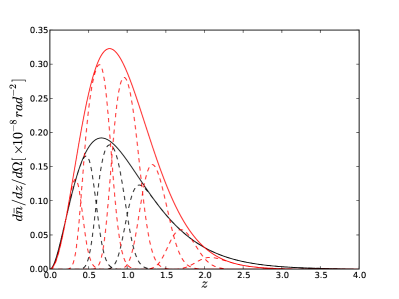
We consider two upcoming weak lensing surveys: the Subaru Hyper Suprime-Cam (HSC) wide field survey hsc , starting in 2013, and that of the EUCLID satellite Laureijs et al. (2011), scheduled to launch in 2020. The main specifications of each experiment are listed in Table 1. For HSC, they are based on Oguri and Takada (2011) and for EUCLID on Amendola et al. (2012). Figure 1 shows the source distributions for the full sample and in the individual bins for each experiment.
IV Effect of uncertainty in photo-z distribution
We use the Fisher matrix formalism (see, e.g., Tegmark et al. (1997)) to forecast constraints from weak lensing on cosmological (and photo-) parameters. The matter power spectra that serve as input for this calculation are computed using the public Boltzmann code CAMB Lewis et al. (2000). We consider a spatially flat universe with dynamical dark energy parametrized by the equation of state function333The varying dark energy equation of state is implemented using the parametrized post-Friedmann (PPF) description Fang et al. (2008). . We thus have eight parameters in total, with fiducial values and , where is the optical depth to reionization. Weak lensing on its own places only weak constraints on the dark energy parameters because of parameter degeneracies. Hence, we combine weak lensing with a forecasted CMB prior from the Planck Planck Collaboration et al. (2013); Planck collaboration et al. (2013); Planck Collaboration et al. (2013) experiment. The Planck Fisher matrix employed here was calculated using the specifications given in Table 2. We assume only multipoles are used and neglect CMB lensing to be on the conservative side and to avoid having to model covariance between the CMB spectra and the lensing spectra. Forecasted constraints much stronger than the ones we will show could be obtained by adding more data sets, but since we would like to isolate as much as possible the constraining power of weak lensing, we will not follow this path. We study the results for different surveys below. While we will consider uncertainties on all parameters, the main quantity of interest will be the dark energy figure of merit (FOM, Albrecht et al. (2006)), defined here as
| (7) |
which is inversely proportional to the area enclosed by a fixed confidence level contour in the plane. Note that, unlike in the definition of the Dark Energy Task Force, we do not marginalize over spatial curvature , but instead fix it to zero.
| - arcmin | - arcmin | ||||
|---|---|---|---|---|---|
| Planck | 100 GHz | 9.5’ | 80 | 114 | 0.8 |
| 143 Ghz | 7.1’ | 46 | 77 | 0.8 | |
| 217 Ghz | 4.7’ | 70 | 122 | 0.8 |
We use linear power spectra as input to calculate the derivatives going into the Fisher matrix and also to compute the covariance matrix of the observables. The latter calculation assumes Gaussianity of the shear field, leading to a diagonal covariance matrix. As we briefly illustrate at the end of Section IV.1, using the information in the non-linear power spectra would lead to significantly stronger forecasted constraints. However, using the non-linear signal, but ignoring the non-Gaussian contributions (specifically the off-diagonal contributions) to the covariance matrix, overestimates the constraining power of weak lensing (see, e.g., Takada and Jain (2009); Kiessling et al. (2011)). While this mainly manifests itself in an underestimate of the multi-dimensional volume of the allowed region in parameter space and individual parameter uncertainties are not affected strongly, we still prefer to present conservative constraints that do not use the information in the non-linear regime at all. Since our main interest in this work is in the dependence of parameter constraints on the level of knowledge of the source redshift distribution, rather than in the exact values of the forecasted uncertainties or FOM, this is not a choice of great consequence.
IV.1 HSC
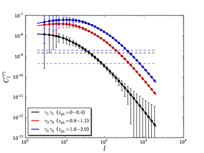
We show the cosmic shear angular power spectra (solid) in our fiducial cosmology, the shape noise power spectra (dashed) and the uncertainty on the binned angular power spectrum in Figure 2. A comparison of the noise and signal spectra shows that the measurement becomes noise dominated above a critical multipole in the range depending on the redshift bin (and on the bin widths chosen). However, by averaging over the large number of available modes, the power spectrum itself can be measured with high accuracy to much higher multipoles, as is shown by the error bars. Using these spectra and their derivatives with respect to cosmological and photo- parameters, we construct a Fisher matrix.
In Table 3, we show the resulting parameter uncertainties and dark energy figure of merit. When perfect knowledge of the photo- parameters is assumed (i.e. fixing the and parameters), adding weak lensing to Planck significantly improves cosmological constraints, causing an increase of the dark energy FOM by a factor 20 and tightening parameter uncertainties by up to a factor of five. The third column, however, shows the results in the case where the 22 photo- parameters are left free. In this case, these parameters are self-calibrated by the cosmic shear data. As can be expected, there is so much freedom in the photo- parameter space, that the weak lensing spectra leave them essentially unconstrained. In other words, the self-calibration is ineffective. As a result, there is a strong degradation of cosmological information, with the parameter uncertainties and dark energy figure of merit returning to their values in the case of Planck only. Thus, when no knowledge of the photo- parameters is assumed, weak lensing does not add any cosmological information compared to the CMB.
In reality, one will have some more knowledge about the photo- distribution, coming from our understanding of the photo- estimator and its calibration with spectroscopic galaxies. This knowledge can in our simplified model be captured by an external prior on the photo- parameters. The question of what prior level is needed to obtain optimal cosmological constraints has been studied in great detail in Ma et al. (2006); Huterer et al. (2006). We find here that if we place a prior on each photo- parameter of , we recover all - most of the cosmological information (FOM ). This is consistent with the findings in the above mentioned works. In Sections V - VII we will show to what extent cross correlations between the source galaxies and an overlapping sample of spectroscopic galaxies can calibrate the photo- parameters and recover the cosmological information in weak lensing. We will there also include the effect of having prior knowledge of the photo- parameters.
Finally, we show in Table 4 the forecasted parameter constraints found when using non-linear matter power spectra (both for the derivatives and the covariances) to calculate the Fisher matrix. Using the non-linear information improves the dark energy figure of merit by a factor of three in the case of known photo- parameters. Moreover, the non-linear power spectrum helps break some of the degeneracy between cosmological parameters and the photo- distribution (as discussed in Hearin et al. (2012)), as even without a prior on the photo- parameters, we now find that lensing (slightly) improves constraints relative to the Planck-only case. For reasons discussed above, we will from now on only use the linear power spectra in our Fisher matrix calculations, but it is good to keep in mind that this is gives rather conservative error estimates.

| Planck | Planck + (known ) | Planck + (“free” ) | |
|---|---|---|---|
| 0.00013 | 0.00011 | 0.00013 | |
| 0.0011 | 0.00069 | 0.0011 | |
| 0.18 | 0.051 | 0.17 | |
| 0.0033 | 0.0027 | 0.0033 | |
| 0.20 | 0.043 | 0.18 | |
| 1.5 | 0.61 | 1.5 | |
| 3.7 | 1.6 | 3.7 | |
| FOM | 0.47 | 9.5 | 0.52 |
| Planck | Planck + (known ) | Planck + (“free” ) | |
|---|---|---|---|
| 0.00013 | 0.000097 | 0.0012 | |
| 0.0011 | 0.00044 | 0.0011 | |
| 0.18 | 0.018 | 0.13 | |
| 0.0033 | 0.0023 | 0.0031 | |
| 0.20 | 0.019 | 0.15 | |
| 1.5 | 0.29 | 0.85 | |
| 3.7 | 0.82 | 1.6 | |
| FOM | 0.47 | 29 | 1.7 |
IV.2 EUCLID
For EUCLID’s lensing survey, the angular power spectra and noise spectra are shown in Figure 3 for a subset of the six tomographic bins, showing that the shear measurements become noise dominated at scales , with , depending on the bin. The error bars on the binned angular spectra are significantly smaller than in the case of HSC, mainly because the ten times larger sky coverage for EUCLID (note, however that because of the different binning choices, one cannot make a direct quantitative comparison between the two figures).
The forecasted parameter uncertainties are given in Table 5. As in the case of HSC, cosmic shear strongly improves cosmological parameter constraints provided that the photo- distribution is known. With EUCLID, the improvement is even more spectacular than before, giving more than a factor 300 increase in FOM. Allowing freedom in the photo- parameters (without an external prior) degrades this information again, although the constraints are still slightly better than with CMB only. The requirement on an external prior on the photo- parameters is a bit more stringent than before, with priors giving figures of merit FOM , so that again subpercent level priors are required to fully exploit the power of weak lensing.
| Planck | Planck + (known ) | Planck + (“free” ) | |
|---|---|---|---|
| 0.00013 | 0.000093 | 0.00013 | |
| 0.0011 | 0.00031 | 0.0011 | |
| 0.18 | 0.013 | 0.13 | |
| 0.0033 | 0.0021 | 0.0031 | |
| 0.20 | 0.011 | 0.12 | |
| 1.5 | 0.14 | 1.4 | |
| 3.7 | 0.36 | 3.6 | |
| FOM | 0.47 | 162 | 1.5 |
V Cross-Correlations (Theory)
We now consider including a galaxy sample with spectroscopic redshifts that covers the same area of the sky as the photometric sample of lensing source galaxies. We stress that the galaxy selection of this sample does not need to overlap with that of the lensing source galaxy sample. All that matters is that the two samples overlap in surveyed volume, so that the galaxy densities trace the same underlying dark matter density. In practice, the spectroscopic sample will most likely consist of more luminous galaxies, with a smaller number density, than the lensing source sample. Allowing for the possibility of dividing both the photometric (label ) and spectroscopic (label ) samples into bins, the auto- and cross-correlations of the overdensities in these bins are given by Equation (4),
where now the kernels are given by
| (8) |
for the bin(s) of photometric source galaxies, where is the galaxy bias of this sample and the normalized redshift distribution, and by
| (9) |
for the spectroscopic bins, with and the bias and distribution of the spectroscopic galaxies. Equation (V) assumes the Limber approximation, which, for the auto-spectra, is appropriate for scales (see Loverde and Afshordi (2008)), where and are the distance to, and width of the redshift slice. McQuinn and White (2013) have recently shown that the Limber approximation is appropriate for the application considered here because most of the information on the source redshift distribution comes from scales well into the regime. To be careful, we choose in our forecast so that the above inequality is satisfied approximately for all included modes (the largest/worst case value of will actually be , but, again, not much information comes from the modes at , so our choice of should suffice for a forecast).
We will divide the spectroscopic sample into a large number of narrow redshift slices and will treat the spectroscopic redshifts as infinitely accurate so that the redshift distribution within a slice has zero weight outside of its defining redshift bounds. In the limit of an infinitely narrow bin at redshift , (with the Dirac delta function), so that the cross correlation with a photometric bin becomes
| (10) |
(note that the Limber approximation can still be applied here because the photometric galaxy distribution is assumed to be spread out in redshift). The cross-correlation is thus proportional to, , the redshift distribution of photometric galaxies in the -th source bin at redshift . This is what motivates cross-correlating with a large number of spectroscopic redshift bins to reconstruct the full function . The spectroscopic galaxy bias in Equation (10) can in principle be obtained from the auto-spectrum of the spectroscopic galaxies. Moreover, the auto-spectrum of the photometric sample may contain additional information on as well. We therefore include in our analysis not just the photo-spec cross correlations (), but also the auto-correlations ( and ).
We will neglect the effect of magnification bias on the auto- and cross-spectra. Magnification bias may act as a double-edged sword (see also McQuinn and White (2013) for an interesting discussion of magnification bias on redshift distribution estimation from cross-correlations). On the one hand, it introduces a correction to Equation (10), so that the cross-spectra are no longer directly proportional to and the correction is non-trivial to model because of the uncertainty in the power law index of the source galaxy number vs. flux threshold relation, . On the other hand, the additional signal may help break the bias degeneracy we will discuss below. We leave further investigation of this possibility for future work.
Of course, to extract all information from the shear/convergence field and the galaxy overdensities, one would use all possible correlations, including for example the cross correlations between shear and the spectroscopic galaxies (galaxy-galaxy lensing). However, we here wish to focus specifically on the use of the spectroscopic galaxies to measure the lensing source distribution. For this reason, we will only consider the , and spectra (in addition to the lensing power spectrum discussed in the previous section and a CMB prior). Moreover, the galaxy overdensities do not only carry information on the redshift distribution, but also direct cosmological information. For the reason explained above however, and to be on the conservative side, we will first calculate a Fisher matrix for the parameters determining , marginalized over the cosmological parameters, using , and . We then add this Fisher matrix to the full Fisher matrix from weak lensing and CMB. This way, we are not including directly any cosmological information encoded in the galaxy clustering. Moreover, any degeneracy between the effect of the source redshift distribution and the effect of cosmological parameters is thus explicitly marginalized over, unlike in previous studies.
V.1 The Role of Galaxy Bias Evolution
Equation (4) shows that all the spectra involving the photometric sample are only sensitive to the bias and the redshift distribution through their product, , giving rise to an exact degeneracy between the two functions Schulz (2010); Bernstein and Huterer (2010); Matthews and Newman (2010); McQuinn and White (2013). This is a potentially serious challenge for the cross-correlation technique. In the following, we will first show how well this technique works in the case where the photometric galaxy bias function is known exactly a priori. We will also study the more realistic case where it is not, and we ask what prior is needed on the galaxy bias for the method to still be useful.
To do this, we will treat the galaxy bias of the source sample as scale independent (appropriate in the linear regime), with redshift evolution modeled as a piecewise constant function in redshift bins, with the value in each bin given by a parameter . We assume a fiducial for all . The binning choice will be discussed for each survey in Section VI. The case of a priori unknown galaxy bias is reproduced by leaving these parameters free, without an external prior. We will then consider two types of bias priors:
-
•
Imposing independent priors on the binned bias parameters. In this case, the required prior depends on the choice of redshift bins in which the galaxy bias is assumed piecewise constant. Specifically, in the limit of a large number of bins (bin width small), the scaling is approximately . To quantify the prior in a binning-independent manner, we thus define
(11) for all redshift bins and will quote the quantity . can be thought of as the prior on the average galaxy bias in a bin of fixed width .
-
•
Assuming the redshift dependence of the bias to be linear in redshift (expanded around a central redshift , the precise choice of which is irrelevant),
(12) and applying a prior to the coefficient,
(13) Here, is the central redshift of the -th galaxy bias redshift bin. We note that the prior on any redshift independent contribution to is irrelevant, as a constant galaxy bias is not degenerate with because of the normalization constraint on the latter function.
We will not study the important question of how to obtain a prior on the bias evolution of the source sample. This is a difficult questions, deserving of a paper of its own. As stated above, the source for the number density per unit area of the source sample, to linear order, is directly proportional to the product (considering the -th tomographic bin) so that this quantity alone can never be used to break the degeneracy. However, as we discussed briefly, there is also a magnification bias contribution. The source term for this contribution is similar in nature to the source for the cosmic shear signal itself. It thus does not depend on galaxy bias and in principle carries information on the source distribution that is independent of galaxy bias. While this information is unfortunately not localized in redshift, it has been found that it may still be possible to use it to constrain the galaxy bias to McQuinn and White (2013). Another way of avoiding the bias degeneracy is to consider the signal in the non-linear regime, where the one-halo term and non-linear bias may carry additional information. Finally, it may be enough to put bounds on the bias evolution from theory, using models and/or simulations to predict the galaxy bias evolution as a function of redshift, luminosity, color, etc. In this work however, we will simply quantify what level of knowledge of the galaxy bias evolution is required for the cross-correlation method to benefit weak lensing studies. These results can then be used as a target for whatever method (or combination of methods) to determine the galaxy bias is used.
Finally, for the galaxy bias of the spectroscopic sample, we again assume a scale independent bias described by a free parameter, for each spectroscopic galaxy bin. We will not impose external priors on the spectroscopic galaxy bias because it can be measured quite accurately using the power spectra of the spectroscopic sample (since there the redshift distribution is assumed to be known perfectly). We describe our (survey dependent) choice of binning in the next section.
VI Spectroscopic Redshift Surveys
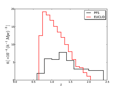
We consider two upcoming galaxy redshift surveys that overlap with the lensing surveys discussed in Section III. For HSC, we study the Prime Focus Spectrograph (PFS) cosmology survey (Ellis et al. (2012)), also with the Subaru telescope, and planned to start in early 2018. Together, these surveys are known as Subaru Measurement of Images and Redshifts (SuMIRe). EUCLID has its own redshift survey, of which we study the complementarity with its lensing survey. Our forecasts of the spectroscopic surveys are based on the specifications in Ellis et al. (2012) (PFS) and Amendola et al. (2012) (EUCLID), We assume the same sky coverage for each spectroscopic survey as for its matching lensing survey (see Table 1). Figure 4 depicts the assumed comoving number density as a function of redshift for each survey.
For the fiducial galaxy bias, we follow Table 2 of Ellis et al. (2012) for PFS, and for EUCLID. We use the binning (7 bins) for PFS and (14 bins) for EUCLID. We remind the reader that each redshift bin has an independent spectroscopic galaxy bias parameter associated with it. Finally, we need to specify the bins that define the photometric galaxy bias parameters. Here we choose for both survey (i.e. coinciding with the PFS spectroscopic bins, but adding a bin at the low and high redshift ends). Note that the bin widths for the are typically smaller than the tomographic redshift bin widths to allow for as general as possible a redshift dependence of .
The redshift bins above are our default choices. We will also consider the effect of varying these choices and will show that our results are robust with respect to the details of the binning of the spectroscopic sample and the binning defining the galaxy bias evolution.
When including galaxy clustering, we apply a cutoff to avoid using modes that are too far into the non-linear regime, , where is the comoving angular diameter distance (as in Section II) to the central redshift of the -th bin. Our standard choice for the comoving wave vector is Mpc, but we will study in detail the dependence of our results. We keep the cutoff in the cosmic shear analysis constant at unless explicitly stated otherwise.
VII Results of Cross-Correlations Technique
VII.1 SuMIRe
VII.1.1 photo- calibration using cross-correlations
We now use the galaxy clustering information in SuMIRe, i.e. the cross-spectra, the auto-spectra (although only the 7 auto-spectra actually contain information because of the absence of overlap between the spectroscopic bins) and the auto-spectra, to constrain the photo- parameters . We marginalize over the cosmological parameters in the process. Because of the large freedom in the redshift evolution of and , the resulting uncertainties in the individual photo- parameters are very large ( and ). However, this does not necessarily mean there is no useful photo- information in the galaxy clustering spectra. What matters is how well the constrain the linear combinations of photo- parameters that are degenerate with the effect of cosmological parameters on the lensing spectra. It is possible for these parameter directions to be well (enough) constrained while the individual and parameters have large error bars.
We next consider explicitly to what extent the photo- information from helps the weak lensing (+Planck) analysis of cosmological parameters. In Table 6, we repeat in the first and last column the cases discussed in Section IV of free photo- parameters (no external priors) and exactly known photo- parameters, respectively. These are the two extreme cases to which we can compare the results using the cross-correlation technique. Ideally, adding the photo- information from will bring the uncertainties and FOM close to the case of perfectly known photo- parameters. What we actually find is shown in the two central columns. The second column shows the results when the galaxy bias of the photometric (source) sample is known perfectly. There is clear improvement, with the dark energy FOM increasing by more than a factor four. However, the result is a long way off from the case of perfectly known photo- parameters. In the third column, we consider the constraints when the redshift evolution of the photometric galaxy bias is unknown a priori (i.e. self-calibrated by the data). We see that leaving free deteriorates constraints, but only by about .
| (“free” ) | + ( known) | + ( unknown) | (known ) | |
|---|---|---|---|---|
| 0.00013 | 0.00012 | 0.00012 | 0.00011 | |
| 0.0011 | 0.0010 | 0.0011 | 0.00069 | |
| 0.17 | 0.11 | 0.12 | 0.051 | |
| 0.0033 | 0.0031 | 0.0032 | 0.0027 | |
| 0.18 | 0.11 | 0.12 | 0.043 | |
| 1.5 | 1.0 | 1.2 | 0.61 | |
| 3.7 | 2.4 | 2.7 | 1.6 | |
| FOM | 0.52 | 2.3 | 1.7 | 9.5 |
VII.1.2 including information from direct photo- calibration
It is instructive to compare the yield of the cross correlation technique to imposing a simple diagonal prior on the photo- parameters. This prior represents the level of calibration that has been achieved for the photo- estimator. For simplicity, we consider the case where we can place a constant prior on all photo- parameters, for all . We find that the obtained figure of merit in Table 6 of FOM for known (unknown) photometric galaxy bias can also be reached with a prior . It is not unlikely that photometric redshifts will be calibrated to this level so that using the galaxy clustering information in the absence of a prior on the photo- parameters is not better than having a prior and not using the information from at all. However, this is not the proper comparison to make. In reality, there will always be some prior on the photo- parameters and we should ask the question how much improvement one gets from adding .
We address this question in Table 7, where we show the dark energy figure of merit with and without for different priors on the photo- parameters. We find that if is larger than , adding galaxy clustering information causes a significant improvement in FOM, but if the prior is better than this, the cross-correlation technique does not add much.
When improves constraints, there is a significant advantage to knowing the galaxy bias. For instance, if the photo- prior is , the FOM is 7.0 if is assumed to be known and 4.7 when it is left free. We tested how well the galaxy bias needs to be known a priori to improve from FOM to (close to) FOM . Applying an independent prior to each bin (see the first bullet point in the discussion in the end of Section V for the definition of the prior), we find that a percent level prior significantly improves the dark energy FOM. For example, gives FOM (approximately halfway between the cases of unknown and known galaxy bias), and gives FOM. Using our second type of galaxy bias prior (the second bullet point in the end of Section V), we find that any prior brings the figure of merit virtually all the way to its optimal value FOM. In other words, merely imposing that the galaxy bias is linear in redshift constrains the bias evolution sufficiently for it to not hinder the determination of the photo- parameters using .
| prior on | (known ) | (unknown ) | |
|---|---|---|---|
| no prior | 0.52 | 2.3 | 1.7 |
| 0.05 | 1.8 | 7.0 | 4.7 |
| 0.02 | 4.4 | 7.5 | 6.0 |
| 0.01 | 7.0 | 8.2 | 7.6 |
| 0.005 | 8.7 | 8.9 | 8.8 |
| 0.0 | 9.5 | 9.5 | 9.5 |
VII.1.3 dependence on and on modeling of photo- distribution
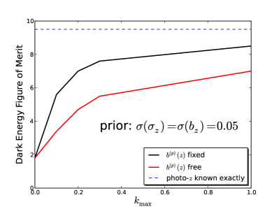
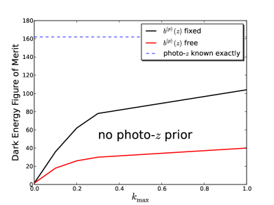
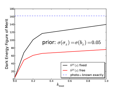
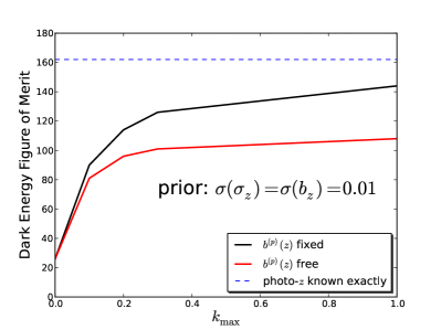
We now consider the dependence of the dark energy figure of merit on the maximum wave vector, , that is included in the . We keep the range of scales used for the lensing analysis fixed (). The results (again for both known galaxy bias and free galaxy bias) are shown in Figure 5. The top left panel gives the figure of merit in the absence of any prior on the photo- parameters, the top right panel describes the case of a (very modest) prior , and the bottom plot is for a stronger prior . In each case, the dependence beyond our default choice Mpc is not very strong.


Finally, we wish to point out that the success of the cross-correlation method depends strongly on how much freedom is allowed in the photo- distribution and its evolution. In the above, we have chosen a fairly general approach with a total of 22 photo- parameters. We now briefly consider the results when we assume the photo- distribution to be redshift independent, i.e. the parameters and are constants. We choose a fiducial (equal to the value of in the previous redshift dependent model at the average redshift ) and , and now have only two free photo- parameters. In this case, the shear-only FOM is already almost four times as large as in the case of redshift dependent photo- parameters (fixing the photo- parameters gives FOM, which is similar to the original result, as expected). Adding the information from , lifts the figure of merit to FOM for fixed (free) photometric galaxy bias. In this more restricted photo- model, the cross-correlation method is thus significantly more powerful. Moreover, the constraints from on the individual photo- parameters are now quite strong (unlike in the more general model), and (here, no galaxy bias prior is assumed).
VII.2 EUCLID
| (“free” ) | + ( known) | + ( unknown) | (known ) | |
|---|---|---|---|---|
| 0.00013 | 0.000096 | 0.00011 | 0.000093 | |
| 0.0011 | 0.00040 | 0.00065 | 0.00031 | |
| 0.13 | 0.025 | 0.050 | 0.013 | |
| 0.0031 | 0.0022 | 0.0025 | 0.0021 | |
| 0.12 | 0.021 | 0.042 | 0.011 | |
| 1.4 | 0.27 | 0.54 | 0.14 | |
| 3.6 | 0.67 | 1.3 | 0.36 | |
| FOM | 1.5 | 62 | 26 | 162 |
VII.2.1 photo- calibration using cross-correlations
We now consider the photo- information in the EUCLID lensing source sample and the EUCLID spectroscopic galaxy sample. Using the cross- and auto-spectra , we find strong direct constraints on a large number of the and parameters, with the uncertainties in the best measured nodes and (assuming no galaxy bias prior). Table 8 (cf. Table 6) shows the effect of the photo- prior from on the cosmological constraints from cosmic shear (+Planck). We again find that the cross-correlation technique significantly improves the weak lensing bounds relative to the case of (a priori) unknown photo- parameters, with the dark energy figure of merit increasing from to for known (unknown) source galaxy bias. As was the case for SuMIRe, the constraints with are still not at the level of cosmic shear with perfectly known source distribution. Moreover, not knowing the bias aversely affects the constraints (decreasing the FOM by ).
| prior on | (known ) | (unknown ) | |
|---|---|---|---|
| no prior | 1.5 | 62 | 26 |
| 0.05 | 3.9 | 101 | 61 |
| 0.02 | 10 | 106 | 75 |
| 0.01 | 26 | 114 | 96 |
| 0.005 | 61 | 127 | 119 |
| 0.002 | 124 | 145 | 143 |
| 0.001 | 150 | 154 | 153 |
| 0.0 | 162 | 162 | 162 |
VII.2.2 including information from direct photo- calibration
The gains from the cross-correlation method shown in Table 8, i.e. FOM, are equivalent to having a photo- prior , showing the strength of this technique for a survey like EUCLID. In Table 9, we show the constraints with and without use of for various external priors on the photo- parameters. Unless this prior is very strong , the cross-correlation method always helps to strongly improve the cosmological constraints.
Considering as an example the case of a photo- prior (as we did for SuMIRe) the figure of merit ranges from FOM , depending on how much information on is available. We find that a diagonal bias prior gives a FOM halfway between these two extremes (FOM), while an even stronger prior is essentially equivalent to knowing the galaxy bias perfectly, lifting the figure of merit to FOM. The bias knowledge requirements are thus stricter than in the case of SuMIRe. On the other hand, imposing to be linear in is already enough to ensure FOM even if no prior is imposed on the slope of this relation (i.e. ).
VII.2.3 dependence on
The dependence of our forecasts on the smallest modes included in the galaxy clustering analysis is shown in Figure 6 for several choices of the external photo- prior . As before the is not particularly strong beyond our default choice of Mpc.
VIII General redshift distribution (no photo- information)
In the previous sections, we have assumed that photometric redshifts are available for the lensing source galaxies, taking into account that the photo- distributions may not be perfectly known. This uncertainty in the photo- distribution translates into uncertainty in the lensing source redshift distribution, which in turn translates into additional uncertainty in cosmological parameters obtained from cosmic shear tomography (or into parameter bias if the effect is not properly modeled). The photo- parameters cannot be properly calibrated by the cosmic shear data itself and we have shown that the resulting degradation in cosmological parameter uncertainties can be very large, depending on the prior knowledge of the photo- parameters.
The main goal of the previous sections (and of this article) was to quantify to what extent cross-correlations between the source galaxies and an overlapping sample of spectroscopic galaxies (in addition to the autocorrelations of these samples) can calibrate the photo- distribution and mitigate the degradation of cosmological parameter estimation from cosmic shear. This addresses directly the question of how useful the cross-correlation technique will be for supporting the constraining power of upcoming lensing surveys. However, because of the assumption of having photo-’s, and because of the joint analysis with a focus on the end product (i.e. cosmological parameters), the analysis thus far does not give much insight into how well in general the cross-correlation method can constrain redshift distributions or what knowledge of the source distribution is required for a lensing analysis. We will address these questions individually in this section. First, we will consider an a priori completely unknown, arbitrary galaxy redshift distribution and study how well it can be measured (Section VIII.1) using the cross- and autocorrelations of the overlapping galaxy number densities (the spectra). We will not assume any photometric redshift information in this section and will pay specific attention to the dependence of our results on our knowledge of galaxy bias evolution. Compared to the rest of this work, Section VIII.1 follows more closely the spirit of previous studies of the subject of using cross-correlations to constrain (source) redshift distributions, see Ho et al. (2008); Newman (2008); Matthews and Newman (2010); Schulz (2010); McQuinn and White (2013); Ménard et al. (2013).
In section VIII.2, we then ask which specific properties (/modes) of the source distribution do we really need to know in order to not weaken cosmological parameter constraints? Comparing how well measures the source distribution to what is the requirement from lensing will then give more insight into when the cross-correlation technique is useful.
Throughout this section, unless otherwise specified, we assume the survey properties of SuMIRe, as described in sections III and VI. While the galaxy sample of which we try to measure the redshift distribution is no longer assumed to have photometric redshift estimates, we will still refer to it as the sample (and refers to the spectroscopic sample). Since for our discussion in Section VIII.1, this sample also no longer has to be a lensing source sample, we will no longer refer to it as the photometric or source sample, but instead call it the target sample.
VIII.1 Measuring a general redshift distribution using the cross-correlation technique
We consider a target sample of galaxies with a distribution based on what would be obtained when applying a photometric redshift cut to the HSC source sample, with . Instead of using the exact resulting distribution, we approximate it by a piecewise constant function defined in bins. The fiducial distributions are depicted by the black lines in Fig. 7 for (top panels) and (bottom). The redshift bins cover the range and have width for .
To quantify how well (the normalized source distribution, as before) can be reconstructed by the cross-correlation method, we treat its value in each bin as a free parameter, , in the Fisher matrix (imposing the normalization condition ). For each bin, we define one slice of spectroscopic galaxies with the same redshift range (thus giving rise to spectroscopic slices). Each spectroscopic bin has a corresponding free galaxy bias parameter (as before). Moreover, in each of these redshift bins, we allow for a free galaxy bias of the target () sample, and, in addition, two free target bias parameters for the bins and .
Thus, in total, we consider auto-spectra (the cross-spectra are zero in the Limber approximation because of the absence of redshift overlap), cross-spectra, and one auto-spectrum as our (prospected) data set and parameters (making 24 or 39 in practice). We wish to stress again that the constraints on the target redshift distribution we will present have any degeneracy with cosmological parameters taken into account and marginalized over. No CMB prior is included so that any degeneracy between and cosmological parameters has to be broken by the galaxy spectra themselves.
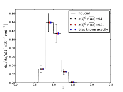
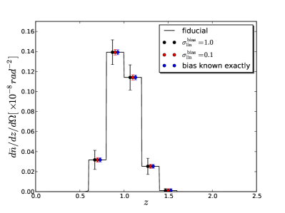


Our main results are shown in Fig. 7. We first consider the case where the target galaxy bias is known exactly (but the cosmological parameters and spectroscopic galaxy bias are marginalized over). The resulting uncertainties in the reconstructed redshift distribution are indicated by the black error bars in the top(bottom) panels for the case (for these errors, there is no difference between the left and right panels). In both cases, errors as small as 2 % can be reached on in the central bins. The uncertainties in do not vary strongly between bins, but the relative uncertainties do because of the lower fiducial values in the bins on the edge of the distribution. In those bins, the relative uncertainties are of order unity or larger. The measurement of the redshift distribution corresponds to a determination of the sample’s mean redshift of (independent of the number of bins ).
The bounds above, however, rely strongly on our assumption that the galaxy bias is known exactly, and will deteriorate when uncertainty in the bias (of the sample) is allowed. In fact, if we allow the bias to be completely free (no prior) in the redshift bins discussed above, the error bars on approach infinity (not shown in the figure) and we are left with no information on the redshift distribution. This was to be expected because of the exact degeneracy between a free and .
We now consider the constraints when independent bias measurements and/or theoretical considerations allow us to place a prior on the galaxy bias evolution, again employing the two types of priors discussed in Section V: a diagonal prior , or a prior on the slope of the bias-redshift relation (assuming linearity), . The left panels show that a weak prior (i.e. , with the bin width) makes it possible again to measure , although still with rather large error bars (typical relative uncertainties 30 %, ). Qualitatively similar results (but somewhat stronger) can be obtained by imposing to be a linear function of redshift and applying a weak prior (right panels). Applying priors an order of magnitude better ( or , see Figure 7) is almost equivalent to knowing the bias exactly for the purpose of redshift distribution reconstruction.
We have shown above that to reconstruct a general galaxy redshift distribution using the cross-correlation technique, it is crucial to have prior knowledge of the galaxy bias evolution. On the bright side, the required bias prior for the method to be successful is not very strict and might be within reach (under the simple assumptions made in this forecast). In the analysis with a cosmic shear focus in the previous sections, by contrast, we had found that a bias prior, while useful, was not as important as here. In particular, even in the absence of such a prior, information on the photo- parameters (and thus on ) could be obtained from the cross-correlation method. The crucial difference, however, in the former analysis is that the true underlying distribution was assumed to be known and that multiple source bins were used. In that case, at the redshifts where the true redshift distributions of neighboring tomographic slices overlap, we are sensitive to both and , where and are the normalized redshift distributions in neighboring bins. The combination (specifically the ratio) of these quantities contains information on the photo- parameters that does not suffer from the bias degeneracy. Therefore, the photo- parameters could be constrained (weakly) even without making assumptions about . Note however that this is only the case because the galaxy bias was assumed to be a function of redshift only. An additional dependence on color for instance would require us to model the bias of galaxies in separate tomographic bins as independent functions, thus reinstating the bias degeneracy.
VIII.2 Lensing requirements on the redshift distribution measurement
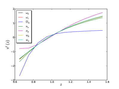
We now isolate the main question on the other end of the procedure of using cross-correlations to improve weak lensing as a cosmological probe: what do we need to know about the lensing source redshift distribution to optimize cosmological parameter constraints from cosmic shear? For simplicity, we will study this question for the case of a single source bin, with the same fiducial redshift distribution (and parametrization in terms of redshift bins) as in the previous subsection. Considering variations from the fiducial , the effects of certain modes on the shear power spectrum will be orthogonal to the effects of cosmological parameters so that uncertainty in these modes would not affect cosmological parameter constraints. We here ask which modes/components of we do need to know because they are degenerate with cosmological parameters. Note that these conclusions will hold only for a given model and might change if we include, e.g., massive neutrinos, etc.
We study this question by considering the cosmological parameter bias induced by assuming the wrong source distribution, with the difference between the assumed and the true distribution. Note that this bias is closely related to the increase in variance in the case where uncertainty in is modeled properly and marginalized over 444Specifically, the requirement for the parameter bias to be small compared to the uncertainty is equivalent to the requirement for the relative change in parameter uncertainty (due to marginalization over uncertainty in ) to be small compared to the uncertainty in in the case where is known..
In the Fisher matrix formalism, the parameter bias is given by
| (14) |
where is the bias in the -th cosmological parameter, the number of parameters not including the parameters describing the source distribution, the Fisher matrix restricted to those parameters, the Fisher matrix for the complete parameter space, and the offset in the binned values of the normalized source redshift distribution . In the limit of a large number of redshift bins, it is convenient to approximate this in terms of continuous functions, and to write the parameter bias as the product of , which is the inner product of with a mode picking out the redshift dependence degenerate with , and a factor , determining the amplitude of the parameter bias. In equations,
| (15) |
with
| (16) |
and the normalized mode defining the inner product (assuming uniform redshift bins for all bins ) given by
| (17) |
(this fully defines , except for its sign, which is arbitrary). An alternative interpretation of is as the coefficient of the mode in an expansion of ,
| (18) |
where the modes in the second term on the right hand side can be part of any basis with
| (19) |
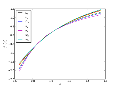
In Figure 8 (left panel), we show the modes for the seven cosmological parameters considered in this work for the case of cosmic shear data with a Planck prior. Strikingly, the mode is almost the same for each parameter except , showing that the only property of that matters is its inner product with this set of two distinct modes. Uncertainty in orthogonal components of would not lead to cosmological parameter bias (or additional uncertainty). The main reason that all these modes are so similar, even though they describe the degeneracy directions with very different cosmological parameters, is the inclusion of the CMB prior. This prior already constrains rather tightly a large number of parameters. Considering the principal components of the CMB-only Fisher matrix, we find that weak lensing only moderately improves three of these (and the other four not at all). Thus, the only variations in that can affect joint cosmological parameter constraints are the ones biasing parameters in this three-dimensional subvolume of the total cosmological parameter space. This significantly narrows down the range of possible modes. In fact, we have checked that, when only the weak lensing data are considered, the modes differ much more strongly, confirming that the reason for them being the same in our case is the inclusion of the CMB prior.
Table 10 shows the parameter bias resulting from an offset in the coefficient (which for a given hardly depends on because of the near-universality of the mode ). The left column shows the change in parameter bias per unit change in , and the right column shows the same quantity normalized by the uncertainty in the cosmological parameter. Judging from the second column, the parameters most affected by a misestimate of (or by uncertainty in) are and . Specifically, we find . This means that if we can limit our misestimate of the relevant mode of to be , then the parameter bias will be small, (note that errors are added in quadrature). Equivalently, limiting the uncertainty , means that the additional uncertainty in is small in case the uncertainty is marginalized over. Since the relevant mode is so similar for each parameter (the only exception being , which has a weak response, , to variations in ), and since is the most strongly affected parameter, the requirement for the other parameters to be negligibly affected is less stringent than this.
| 0.00016 | 1.3 | |
| -0.0021 | -1.9 | |
| -0.033 | -0.20 | |
| 0.0019 | 0.58 | |
| 0.092 | 0.51 | |
| 4.7 | 3.7 | |
| -16 | -6.4 |
In summary, in the simple case considered above of cosmic shear in a single tomographic bin, the requirement on our knowledge of the source distribution is
| (20) |
where is given by the cyan curve in Figure 8. In the present case (single lensing source bin with CMB prior, etc.), this constraint is more or less satisfied even when the source distribution is self-calibrated using the lensing information (i.e. no external information from cross correlations). Specifically, we find (the uncertainties of the other coefficients are in the range for all parameters, but we have confirmed that is the parameter most affected by uncertainty in ) so that even without additional information, the uncertainty in does not affect the WL+Planck cosmological constraints much.
However, upon further inspection, the reason for this is simply that a single source bin at , with HSC-like survey specifications, does not add much information to the CMB-only case even with perfect knowledge of . Variations in thus do not have a large effect on the final cosmological constraints and the requirement on the knowledge of is weak. We therefore consider next the more interesting case where the lensing measurement does add significant information to the Planck-only case. We achieve this by simply considering a full-sky shear measurement of a source sample with the same properties as above (except for the sky coverage). The resulting modes are shown in the right panel of Figure 8 and the response of cosmological parameters to variations in the coefficients in Table 11. The modes are now even more similar across the set of cosmological parameters. Since now the lensing contributes more to parameter constraints, they are more sensitive to uncertainty in , as is shown best in the second column of Table 11.
The strictest requirement on again comes from . In order not to bias this parameter significantly, is needed. The uncertainty in from the shear power spectrum itself (+ Planck) is (in general, ). Thus, marginalizing over the uncertainty in , the constraint on is weakened by a factor compared to the case of known (). Other parameter uncertainties increase by smaller factors, but overall this is a significant degradation of cosmological information. On the other hand, using the cross and auto spectra (as used in the previous subsection, 1500 deg2 sky coverage), fixing , we find a constraint (in fact, for all parameters, ) so that the effect of on parameter constraints becomes negligible.
| 0.00021 | 1.7 | |
| -0.0036 | -3.6 | |
| -0.47 | -4.4 | |
| 0.0058 | 1.9 | |
| -0.43 | -4.1 | |
| 7.7 | 7.6 | |
| -21 | -9.2 |
VIII.3 Summary
The study above has broken down the procedure followed in this paper into its two main components.
-
•
Weak lensing constraints are weakened if is not known accurately enough, and we have quantified above which properties of need to be constrained, and with what precision. We have done this for the particular case of a single source distribution (no tomography). The specific results will depend on many assumptions, but the methodology above is of general application. Moreover, a result that appears robust against changes in fiducial source redshift distribution is that the main property of that affects cosmological constraints is an inner product of with a mode of the shape depicted in Figure 8 that crosses zero only once. The dominant effect of such a mode is to shift the average redshift of the distribution.
-
•
The other component, discussed in subsection VIII.1, is how well the cross-correlation technique can provide an external measurement of . We have shown that this method can provide a strong measurement of , provided that sufficient knowledge of the galaxy bias evolution is available. This measurement of can then be propagated to a measurement of the mode coefficients (inner products) , which can be compared to the requirement of a cosmic shear cosmology analysis. The quantitative results are strongly dependent on survey and sample assumptions, but we have given an example for illustration. In general, it appears that with sufficient knowledge of , the cross-correlation technique provides enough information to restore the power of cosmic shear to its level in the case of perfectly known , but the specific galaxy bias prior requirement differs from case to case.
The analysis in this section takes a rather different approach than our main forecasts for realistic surveys in the previous sections, but we hope that by isolating the phenomenology involved in the Fisher forecasts of those sections, we have provided a bit more insight into those constraints.
IX Discussion and Conclusions
We have studied the use of cross-correlations between lensing source galaxies and an overlapping sample of spectroscopic galaxies as a method to measure the source galaxy redshift distribution and to thus improve cosmic shear as a cosmological probe. We used the Fisher matrix formalism to for the first time directly forecast the impact on cosmological constraints of this cross-correlation technique, focusing on dark energy constraints from two types of future experiments: a ground based SuMIRe-like survey (HSC lensing + PFS redshift survey) and a space based EUCLID-like survey. For the main results of this paper, we have considered the scenario where the source galaxies have photometric redshifts, which are used to divide the source sample into tomographic bins, so that the redshift distribution in each bin is known perfectly (only) in the limit where the photo- distribution is known exactly.
We first considered weak lensing constraints in the absence of galaxy density cross-correlation information and have shown that cosmic shear can strongly improve dark energy constraints relative to the case of (unlensed) CMB information only (increasing the dark energy figure of merit by factors of 20-300 for HSC-EUCLID), if and only if the photo- parameters (defining the photo- distribution) are known well. We confirmed the well known result from the literature that in order for weak lensing to reach its full potential as a dark energy probe, the photo- distribution needs to be known at the level .
We then considered to what extent the cross-correlation technique can restore the cosmology constraints from weak lensing by measuring the photo- parameters (we remind the reader that we do not use information on cosmological parameters present in the galaxy cross- and auto-spectra, only the information on the source redshift distribution). We list some key results below.
-
•
Starting with the case where there is no prior knowledge of the photo- parameters, the cross-correlation technique results in strong improvements in the forecasted weak lensing uncertainties. For the SuMIRe-like survey, the effect of the cross-correlation information on the dark energy FOM is equivalent to placing a prior (known galaxy bias - free galaxy bias) on the photo- parameters at all redshifts. For the EUCLID-like survey, using the cross-correlations is equivalent to an even better known photo- distribution, . One reason for the increased success of the method in the case of EUCLID is the fact that EUCLID’s spectroscopic survey has much better coverage of the low redshift end of the distribution.
-
•
In the more realistic case where some level of prior knowledge of the photo- distribution is assumed, e.g. coming from calibration of the photo- estimator using galaxy spectra for a representative subsample of the source galaxies, the cross-correlation approach still strongly improves constraints, unless the prior on the photo- distribution is very strong. For example, for SuMIRe, with a prior on the photo- parameters, including the information from the cross-correlation technique improves the dark energy FOM by more than a factor (known galaxy bias - free galaxy bias) relative to the case without this information. For EUCLID, with the same photo- prior, the gains are even more spectacular, giving a factor improvement. Only when the photo- calibration is better than for SuMIRe (EUCLID), do the benefits from the cross-correlation method become negligible (). We do note that, even in the cases where the dark energy figure of merit is significantly enhanced by use of the cross-correlation information, it does not reach all the way to the value that could have been obtained if the source redshift distribution were known perfectly.
-
•
The power of the cross-correlation method, however, depends strongly on the assumed knowledge of the galaxy bias evolution of the source sample. We have modeled the galaxy bias as a free function of redshift, defined by independent bias values in a large number of redshift bins and have considered both the case of a priori completely unknown values of these bias parameters and various levels of prior knowledge (including knowing the galaxy bias exactly). For example, again in the case with a photo- calibration at the level, assuming exact knowledge of yields a larger dark energy FOM (and therefore effective survey volume) for SuMIRe (EUCLID) than when no prior knowledge of is assumed. The optimal constraints of the known bias case can be approached by imposing a bias prior () for SuMIRe (EUCLID). This prior can be seen as the prior on the galaxy bias per redshift bin of width , see Section V.1. As discussed in Section VIII.1, the reason that the cross-correlation technique still provides some information in the absence of a galaxy bias prior can be explained by our simple model for the source distribution, which allows the extraction of information from the overlap in tomographic bins that does not suffer from the bias degeneracy. This would likely not work in practice however.
To gain more insight in the results described above, we have included a section (Section VIII) showing to what degree a single redshift distribution can be reconstructed in redshift bins using the cross-correlation method, in the absence of photo- information. In this case, we have confirmed that without any galaxy bias prior, no information on the sample’s redshift distribution can be obtained. We have found that a reasonable reconstruction of the distribution ( uncertainties) can be achieved with a bias prior . A prior an order of magnitude smaller results in an optimal (in the sense that it can not be improved by tightening the prior even more) reconstruction of the redshift distribution, with error bars in individual redshift bins as small as .
We have in the same section determined, for each cosmological parameter, which component (or mode) of the source redshift distribution
needs to be known in order to not bias that parameter in a cosmic shear study.
We have demonstrated that, when weak lensing is combined with the CMB,
this mode varies very little between different cosmological parameters and predominantly describes a shift in the average redshift of the distribution.
With only weak lensing data (including the CMB prior, as always), the coefficient of this mode is typically not well measured,
leading to a degradation of cosmological constraints. However, the galaxy cross- (and auto-)spectra are capable of measuring this coefficient
much more accurately, thus explaining how the cross-correlation technique aids weak lensing as a cosmological probe.
In summary, our results confirm that using cross-correlations to constrain the source redshift distribution (whether on its own or, more realistically, in combination with photometric redshifts) has the potential to significantly improve the constraining power of upcoming weak lensing surveys, although the level of success depends strongly on our ability to constrain the bias evolution of the source galaxies. While these are very encouraging results, we have made several simplifications and additional research is needed to clarify how the method is affected by changes in these assumptions. For example, it would be interesting to go beyond the Gaussian description of the photo- distribution and include, among other things, outliers in the distribution. It would also be useful to study extensions of the cosmological model considered in this work, including massive neutrinos, modifications of gravity, etc. Moreover, it is not clear what the role will be of magnification bias (whether it will weaken the cross-correlation approach or improve it by helping break the degeneracy between redshift distribution and galaxy bias). Finally, the fact that the photo- parameters could be measured even in the absence of a galaxy bias prior really hinges on the assumption that the galaxy bias is a function of redshift only. A more general treatment would allow for dependence on galaxy properties such as color (so that the bias of galaxies in different tomographic bins at the same true redshift is not necessarily equal), which, if left otherwise unconstrained by additional data or modeling, would worsen the constraints from the cross-correlation method.
X acknowledgments
The authors thank Carlos Cunha, Patrick MacDonald, Jeffrey Newman, David Schlegel, David Spergel and Masahiro Takada for useful discsussions. Part of the research described in this paper was carried out at the Jet Propulsion Laboratory, California Institute of Technology, under a contract with the National Aeronautics and Space Administration. This work is supported by NASA ATP grant 11-ATP-090.
References
- Albrecht et al. (2006) A. Albrecht, G. Bernstein, R. Cahn, W. L. Freedman, J. Hewitt, W. Hu, J. Huth, M. Kamionkowski, E. W. Kolb, L. Knox, et al., ArXiv Astrophysics e-prints (2006), eprint arXiv:astro-ph/0609591.
- Bartelmann and Schneider (2001) M. Bartelmann and P. Schneider, Physics Reports 340, 291 (2001), eprint arXiv:astro-ph/9912508.
- Hoekstra and Jain (2008) H. Hoekstra and B. Jain, Annual Review of Nuclear and Particle Science 58, 99 (2008), eprint 0805.0139.
- Weinberg et al. (2012) D. H. Weinberg, M. J. Mortonson, D. J. Eisenstein, C. Hirata, A. G. Riess, and E. Rozo, ArXiv e-prints (2012), eprint 1201.2434.
- Massey et al. (2007a) R. Massey, J. Rhodes, A. Leauthaud, P. Capak, R. Ellis, A. Koekemoer, A. Réfrégier, N. Scoville, J. E. Taylor, J. Albert, et al., Astrophys.J.Supp. 172, 239 (2007a), eprint arXiv:astro-ph/0701480.
- Massey et al. (2007b) R. Massey, J. Rhodes, R. Ellis, N. Scoville, A. Leauthaud, A. Finoguenov, P. Capak, D. Bacon, H. Aussel, J. Kneib, et al., Nature 445, 286 (2007b), eprint arXiv:astro-ph/0701594.
- Fu et al. (2008) L. Fu, E. Semboloni, H. Hoekstra, M. Kilbinger, L. van Waerbeke, I. Tereno, Y. Mellier, C. Heymans, J. Coupon, K. Benabed, et al., Astronomy & Astrophysics 479, 9 (2008), eprint arXiv:0712.0884.
- Schrabback et al. (2009) T. Schrabback, J. Hartlap, B. Joachimi, M. Kilbinger, P. Simon, K. Benabed, M. Bradač, T. Eifler, T. Erben, C. D. Fassnacht, et al., ArXiv e-prints (2009), eprint arXiv:0911.0053.
- Huff et al. (2011) E. M. Huff, T. Eifler, C. M. Hirata, R. Mandelbaum, D. Schlegel, and U. Seljak, ArXiv e-prints (2011), eprint 1112.3143.
- Kilbinger et al. (2013) M. Kilbinger, L. Fu, C. Heymans, F. Simpson, J. Benjamin, T. Erben, J. Harnois-Déraps, H. Hoekstra, H. Hildebrandt, T. D. Kitching, et al., Mon. Not. R. Astron. Soc. 430, 2200 (2013), eprint 1212.3338.
- Heymans et al. (2013) C. Heymans, E. Grocutt, A. Heavens, M. Kilbinger, T. D. Kitching, F. Simpson, J. Benjamin, T. Erben, H. Hildebrandt, H. Hoekstra, et al., ArXiv e-prints (2013), eprint 1303.1808.
- (12) http://www.darkenergysurvey.org
- (13) http://www.naoj.org/Projects/HSC/index.html
- (14) http://www.lsst.org/
- Laureijs et al. (2011) R. Laureijs, J. Amiaux, S. Arduini, J. . Auguères, J. Brinchmann, R. Cole, M. Cropper, C. Dabin, L. Duvet, A. Ealet, et al., ArXiv e-prints (2011), eprint 1110.3193.
- Ma et al. (2006) Z. Ma, W. Hu, and D. Huterer, Astrophys. J. 636, 21 (2006), eprint arXiv:astro-ph/0506614.
- Huterer (2002) D. Huterer, Phys. Rev. D 65, 063001 (2002), eprint arXiv:astro-ph/0106399.
- Huterer et al. (2004) D. Huterer, A. Kim, L. M. Krauss, and T. Broderick, Astrophys. J. 615, 595 (2004), eprint arXiv:astro-ph/0402002.
- Huterer et al. (2006) D. Huterer, M. Takada, G. Bernstein, and B. Jain, Mon. Not. R. Astron. Soc. 366, 101 (2006), eprint arXiv:astro-ph/0506030.
- Cunha et al. (2012) C. E. Cunha, D. Huterer, H. Lin, M. T. Busha, and R. H. Wechsler, ArXiv e-prints (2012), eprint 1207.3347.
- Newman (2008) J. A. Newman, Astrophys. J. 684, 88 (2008), eprint 0805.1409.
- Cai and Bernstein (2012) Y.-C. Cai and G. Bernstein, Mon. Not. R. Astron. Soc. 422, 1045 (2012), eprint 1112.4478.
- Gaztañaga et al. (2012) E. Gaztañaga, M. Eriksen, M. Crocce, F. J. Castander, P. Fosalba, P. Marti, R. Miquel, and A. Cabré, Mon. Not. R. Astron. Soc. 422, 2904 (2012), eprint 1109.4852.
- Matthews and Newman (2010) D. J. Matthews and J. A. Newman, Astrophys. J. 721, 456 (2010), eprint 1003.0687.
- Schulz (2010) A. E. Schulz, Astrophys. J. 724, 1305 (2010), eprint 0910.3683.
- Matthews and Newman (2012) D. J. Matthews and J. A. Newman, Astrophys. J. 745, 180 (2012), eprint 1109.2121.
- McQuinn and White (2013) M. McQuinn and M. White, ArXiv e-prints (2013), eprint 1302.0857.
- Schneider et al. (2006) M. Schneider, L. Knox, H. Zhan, and A. Connolly, Astrophys. J. 651, 14 (2006), eprint arXiv:astro-ph/0606098.
- Bernstein and Huterer (2010) G. Bernstein and D. Huterer, Mon. Not. R. Astron. Soc. 401, 1399 (2010), eprint 0902.2782.
- Phillipps (1985) S. Phillipps, Mon. Not. R. Astron. Soc. 212, 657 (1985).
- Masjedi et al. (2006) M. Masjedi, D. W. Hogg, R. J. Cool, D. J. Eisenstein, M. R. Blanton, I. Zehavi, A. A. Berlind, E. F. Bell, D. P. Schneider, M. S. Warren, et al., Astrophys. J. 644, 54 (2006), eprint arXiv:astro-ph/0512166.
- Ho et al. (2008) S. Ho, C. Hirata, N. Padmanabhan, U. Seljak, and N. Bahcall, Phys. Rev. D 78, 043519 (2008), eprint 0801.0642.
- Ménard et al. (2013) B. Ménard, R. Scranton, S. Schmidt, C. Morrison, D. Jeong, T. Budavari, and M. Rahman, ArXiv e-prints (2013), eprint 1303.4722.
- Ellis et al. (2012) R. Ellis, M. Takada, H. Aihara, N. Arimoto, K. Bundy, M. Chiba, J. Cohen, O. Dore, J. E. Greene, J. Gunn, et al., ArXiv e-prints (2012), eprint 1206.0737.
- Limber (1954) D. N. Limber, Astrophys. J. 119, 655 (1954).
- Ma and Bernstein (2008) Z. Ma and G. Bernstein, Astrophys. J. 682, 39 (2008), eprint 0712.1562.
- Hearin et al. (2010) A. P. Hearin, A. R. Zentner, Z. Ma, and D. Huterer, Astrophys. J. 720, 1351 (2010), eprint 1002.3383.
- Pen et al. (2000) U.-L. Pen, J. Lee, and U. Seljak, Astrophys. J. Lett. 543, L107 (2000), eprint arXiv:astro-ph/0006118.
- Catelan et al. (2001) P. Catelan, M. Kamionkowski, and R. D. Blandford, Mon. Not. R. Astron. Soc. 320, L7 (2001), eprint arXiv:astro-ph/0005470.
- Hirata and Seljak (2004) C. M. Hirata and U. Seljak, Phys. Rev. D 70, 063526 (2004), eprint arXiv:astro-ph/0406275.
- Heavens et al. (2000) A. Heavens, A. Refregier, and C. Heymans, Mon. Not. R. Astron. Soc. 319, 649 (2000), eprint arXiv:astro-ph/0005269.
- Oguri and Takada (2011) M. Oguri and M. Takada, Phys. Rev. D 83, 023008 (2011), eprint 1010.0744.
- Amendola et al. (2012) L. Amendola, S. Appleby, D. Bacon, T. Baker, M. Baldi, N. Bartolo, A. Blanchard, C. Bonvin, S. Borgani, E. Branchini, et al., ArXiv e-prints (2012), eprint 1206.1225.
- Tegmark et al. (1997) M. Tegmark, A. Taylor, and A. Heavens, Astrophys.J. 480, 22 (1997).
- Lewis et al. (2000) A. Lewis, A. Challinor, and A. Lasenby, Astrophys.J. 538, 473 (2000), eprint arXiv:astro-ph/9911177.
- Fang et al. (2008) W. Fang, W. Hu, and A. Lewis, Phys. Rev. D 78, 087303 (2008), eprint 0808.3125.
- Planck Collaboration et al. (2013) Planck Collaboration, P. A. R. Ade, N. Aghanim, C. Armitage-Caplan, M. Arnaud, M. Ashdown, F. Atrio-Barandela, J. Aumont, C. Baccigalupi, A. J. Banday, et al., ArXiv e-prints (2013), eprint 1303.5062.
- Planck collaboration et al. (2013) Planck collaboration, P. A. R. Ade, N. Aghanim, C. Armitage-Caplan, M. Arnaud, M. Ashdown, F. Atrio-Barandela, J. Aumont, C. Baccigalupi, A. J. Banday, et al., ArXiv e-prints (2013), eprint 1303.5075.
- Planck Collaboration et al. (2013) Planck Collaboration, P. A. R. Ade, N. Aghanim, C. Armitage-Caplan, M. Arnaud, M. Ashdown, F. Atrio-Barandela, J. Aumont, C. Baccigalupi, A. J. Banday, et al., ArXiv e-prints (2013), eprint 1303.5076.
- Takada and Jain (2009) M. Takada and B. Jain, Mon. Not. R. Astron. Soc. 395, 2065 (2009), eprint 0810.4170.
- Kiessling et al. (2011) A. Kiessling, A. N. Taylor, and A. F. Heavens, Mon. Not. R. Astron. Soc. 416, 1045 (2011), eprint 1103.3245.
- Hearin et al. (2012) A. P. Hearin, A. R. Zentner, and Z. Ma, JCAP 4, 034 (2012), eprint 1111.0052.
- Loverde and Afshordi (2008) M. Loverde and N. Afshordi, Phys. Rev. D 78, 123506 (2008), eprint 0809.5112.