TraMoS project III: Improved physical parameters, timing analysis, and star-spot modelling of the WASP-4b exoplanet system from 38 transit observations.

Abstract

We report twelve new transit observations of the exoplanet WASP-4b from the Transit Monitoring in the South Project (TraMoS) project. These transits are combined with all previously published transit data for this planet to provide an improved radius measurement of $R_{p}=1.395\pm 0.022~{}R_{jup}$ and improved transit ephemerides. In a new homogeneous analysis in search for Transit Timing Variations (TTVs) we find no evidence of those with RMS amplitudes larger than $20$ seconds over a 4-year time span. This lack of TTVs rules out the presence of additional planets in the system with masses larger than about $2.5~{}M_{\earth}$, $2.0~{}M_{\earth}$ and $1.0~{}M_{\earth}$ around the 1:2, 5:3 and 2:1 orbital resonances. Our search for the variation of other parameters, such as orbital inclination and transit depth also yields negative results over the total time span of the transit observations. Finally we perform a simple study of stellar spots configurations of the system and conclude that the star rotational period is about 34 days.

1 Introduction

Since the discovery of the first extrasolar planet around the Sun-like star 51-Peg via radial velocities (Mayor & Queloz, 1995), a number of systematic extrasolar planet searches have spread adopting a wide variety of techniques, of which the radial velocity method is still the most prolific approach. The transit technique is currently the second most successful, with the detection of over 290 systems with confirmed planet detection. Of these, most are Hot-Jupiters (Jupiter-mass objects with orbital periods of a few days). Just recently, space missions such as Kepler and Corot have started to expand transit discoveries to planets smaller than $50~{}M_{\earth}$.

Transiting planets provide a wealth of information about their systems. For instance, transits are currently the only tool to measure the planet-to-star radius ratio and orbital inclination. Combined with radial velocity results, those parameters allow the determination of the absolute mass of the planet and its mean density. Another type of study that can be conducted via transiting planets is the search of unseen companions in the system. Those companions introduce variations in the orbital period of the transiting planet (Miralda-Escudé, 2002; Agol et al., 2005; Holman & Murray, 2005), which can be detected by monitoring the systems in search for Transit Timing Variations (TTVs). This TTV technique has the potential of finding planets in the Earth-mass regime and even exomoons (Kipping, 2009).

In addition, Silva-Valio (2008) and Sanchis-Ojeda et al. (2011) have pointed out that observations of star-spot occultations during closely-spaced transits can be used to not only estimate the rotation period of the host star, but also to measure alignment differences between the rotation axis of the star and the orbital axis of the planet.

As part of the Transit Monitoring in the South (TraMoS) project (Hoyer et al., 2011, 2012), we are conducting a photometric monitoring survey of transits observable from the Southern Hemisphere. The aim of this project is to perform a careful and homogeneous monitoring of exoplanet transits trying to minimize systematics and reduce uncertainties in the transit parameters, such as the transit mid-time, following the approach of using high-cadence observations and the same instruments and setups.

In the framework of the TraMoS project we present twelve new transit observations of the exoplanet WASP-4b. This was the first exoplanet detected by the WASP-South survey in 2008. A that time, Wilson et al. (2008, hereafter W08) reported a Hot-Jupiter ($P=1.34$ days) with a mass of $M_{P}=1.22^{+0.09}_{-0.08}~{}M_{J}$ and a planetary radius of $R_{p}=1.42^{+0.07}_{-0.04}~{}R_{J}$ orbiting a G7V southern star. This discovery paper included WASP photometry, two additional transit epochs (observed in September 2007), and radial velocities measurements.

Gillon et al. (2009, hereafter G09), added to the follow-up of this exoplanet a VLT/FORS2 light curve observed in October 2007 with a z-GUNN filter. Using a reanalysis of the W08 data they found no evidence of period variability. Winn et al. (2009, hereafter W09), presented two new high-quality transits observed in 2008 with the Baade Telescope (one of the twin 6.5-m Magellan telescopes at Las Campanas Observatory) using a z-band filter. Four new transit epochs were reported shortly after by Southworth et al. (2009, hereafter S09), with the 1.54-m Danish Telescope at La Silla Observatory using a Cousins-R filter during 2008. Sanchis-Ojeda et al. (2011, hereafter S011), using four new transit light curves observed during 2009, interpreted two anomalies in the photometry as starspot occultations by the planet and concluded from that result that the stellar rotation axis is nearly aligned with the planet’s orbital axis. This result agrees with the observations of the Rossiter-McLaughlin effect for this system by Triaud et al. (2010). Later, two new transits of WASP-4b were reported by Dragomir et al. (2011, hereafter D11), with data from the 1-m telescope at Cerro Tololo Inter-American Observatory (V-band and R-band filter). Most recently, Nikolov et al. (2012, hereafter N12) observed three transits simultaneously in the Sloan g’, r’, i’ and z’ filters with the Gamma Ray burst Optical and Near-infrared Detector (GROND) at the MPG/ESO-2.2 m telescope at La Silla Observatory.

In this work we present twelve new transits observations. We combined these new light curves with all the previously available light curves (twenty-six additional light curves) and reanalyzed them to provide a new homogeneous timing analysis of the transits of WASP-4b and to place stronger constraints to the mass of potential perturbers in the main orbital resonances with this planet. We also search the entire dataset for signs of stellar spots that would help improve the conclusions of S011.

In Section 2 and 3 we describe the new observations and the data reduction. Section 4 details the modelling of the light curves and in Section 5 we present the timing analysis and discuss the mass limits for unseen perturbers. In section 6 we discuss the occultations of stellar spots by the planet. Finally, we present our conclusions in Section 7.

2 Observations

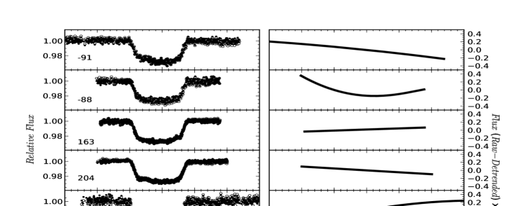
Figure 1: Left: Detrended light curves (black points) plotted over the raw light curves (gray points) to illustrate the amount of detrending applied before the transit modelling using MCMC. The epoch of each transit is shown in the bottom left of each panel. Right: The flux difference (x 100 times) between the raw and detrended light curves.

2.1 The instruments

As mentioned before, the TraMoS project has undertaken a photometric campaign to follow-up transiting planets observable from the Southern Hemisphere. Our goal is to use high cadence observations minimizing change of instruments to reduce systematics and therefore, based on an homogeneous analysis, obtain the most precise values of the light curve parameters, such as the central time of the transit, the orbital inclination and the planet radius, among others.

The observations we present in this work were performed with the Y4KCam on the SMARTS 1-m Telecope at Cerro Tololo Inter-American Observatory (CTIO) and with the SOAR Optical Imager (SOI) at the 4.2-m Southern Astrophysical Research (SOAR) telescope in Cerro Pachón. The epochs of four of the transits we present here coincide with previous published data (see Table 1).

We have taken advantage of the $20\times 20$ squared arcminute of Field of View (FoV) of the Y4KCam, which is a $4064\times 4064$ CCD camera with a pixel scale of 0.289 arcsec pixel^-1, which despite its large dimensions allows to use a readout time of only $\sim 16/5$ sec when using the 2x2/4x4 binning mode (compared with the $46$ sec of the unbinned readout time). The SOI detector is composed of two E2V mosaics of $4096\times 2048$ pixels with a scale of 0.077 arcsec pixel^-1. The SOI has a FoV of $5.2\times 5.2$ squared arcminutes and allows a readout time of only $\sim 11$ sec after binning 2x2 ($20.6$ sec is its standard readout time).

As part of the TraMoS project we have observed a total of 12 transits of WASP-4b, between August 2008 and September 2011. Three transits were observed with the SOI at the SOAR telescope and the remaining nine were observed with the Y4KCAM at the 1-m CTIO telescope. The first ten transits were observed using a Bessell I or Cousins I filter. For the 2011 transit observations we use the 4x4 binning mode of the Y4KCam and a Cousins R filter. The observing log is summarized in Table 1.

All the transits were fully covered by our observations except for some portions of the $E=754$, $482$ and $-62$ transits that were lost due to technical failures (see Figure 2). The before-transit and ingress portions of the $E=-71$ transit were not observed, but after $phase=-0.034$ (where $phase=0$ is defined as the phase of the mid-transit) the observation of the transit was done without interruption.

Table 1: Details about each of the new transit epoch observation presented in this work.

UT date	Epochb	Telescope/Instrument	Filter	Binning	Average	Detrending	$K_{\textit{RMS}}$
					exptime (sec)
2008-08-23a	-91	1-mt SMART/Y4KCam	Cousins I	2x2	20	3	0.78
2008-08-23a	-91	SOAR/SOI	Bessell I	2x2	7	–	–
2008-08-27	-88	1-mt SMART/Y4KCam	Cousins I	2x2	20	1+3	0.90
2008-09-19	-71	1-mt SMART/Y4KCam	Cousins I	2x2	20	–	–
2008-09-23a	-68	1-mt SMART/Y4KCam	Cousins I	2x2	20	–	–
2008-10-01a	-62	1-mt SMART/Y4KCam	Cousins I	2x2	26	–	–
2009-07-29	163	SOAR/SOI	Bessell I	2x2	8	2	0.91
2009-09-22	204	SOAR/SOI	Bessell I	2x2	10	2	0.87
2009-10-28	231	1-mt SMART/Y4KCam	Bessell I	2x2	14	–	–
2010-09-29	482	1-mt SMART/Y4KCam	Cousins I	2x2	14	1+3	0.96
2011-09-24	751	1-mt SMART/Y4KCam	Cousins R	4x4	20	1+3	0.95
2011-09-28	754	1-mt SMART/Y4KCam	Cousins R	4x4	20	–	–
a These epochs have been already observed by other authors. b Epochs are caculated using the ephemeris equation
from Dragomir et al. (2011). c Detrending using (1) airmass, (2) linear or (3) quadratic regression.

3 Data Reduction

The trimming, bias and flatfield correction of all the collected data was performed using custom-made pipelines specifically developed for each instrument.

The Modified Julian Day (JD-2400000.5) value was recorded at the start of each exposure in the image headers. In the SMARTS telescope, the time stamp recorded in the header of each frame is generated by a IRIG-B GPS time synchronization protocol connected to the computers that control the instrument. The SOAR telescope data use the time values provided by a time service connected to the instrument. We confirmed that these times coincide with the time of the Universal Time (UT) reference clock within 1 second. The time stamp assigned to each frame corresponds to the Julian Day at the start of the exposure plus 1/2 of the integration time of each image.

For the photometry and light curve generation we used the same procedure described in Hoyer et al. (2012). That is, we performed a standard aperture photometry where the optimal sky-aperture combination was chosen based on the RMS minimization of the differential light curves of the target and the reference stars. For this analysis we excluded the ingress and egress portions of the light curves, i.e. we used only the out-of transit and in-transit data. The final light curves were generated computing the ratio between the target flux and the average flux of the best 1 to 3 comparison stars.

In order to detrend the light curves, we searched for correlations of the out-of-transit flux ($F_{OOT}$) with the X-Y CCD coordinates of the target, airmass and/or time. Trends are identified as such when the correlation coefficient values are larger than the RMS of the out-of-transit points. To remove the trends, we applied linear or quadratic regressions fits, which were subtracted from the light curve only when we detect that RMS of the $F_{OOT}$ is improved. Otherwise no subtraction is applied. The RMS after detrending are $3-22\%$ lower than on the raw light curves. A posteriori we have checked that doing this detrending previous to modelling our light curves does not introduce any bias or differences in the estimated parameters and its uncertainties. In the last two columns of Table 1 we show which detrending was applied and the value $K_{{\it RMS}}$, which corresponds to the ratio of the $F_{OOT}$ RMS after and before removing the trends to illustrate the improvement in the RMS by the detrending. Therefore, the values of $K_{RMS}$ indicate how much the dispersion of the light curves changes after detrending. When no numerical values of $K_{{\it RMS}}$ is shown means that no significant systematic trend with any of the parameters searched was found. Also, to illustrate the amount of detrending applied for each light curve in left panels of Figure 1 we show the detrended over the raw light curves and in the right-side of the same figure we also show the differences in flux (magnified by 100 times) between the light curves before and after detrending.

4 Light Curve Modelling

In a first step we performed a modelling of the 12 new light curves we present in this work and the 26 available light curves of the WASP-4 system from other authors. The goal of this first analysis is to determine transit parameters single values from each light curve. With these values we search for variations in 4 years time span in parameters such as the central time of the transits, the orbital inclination and/or the transit’s depth. Variations in these parameters can be indicative of the presence of a perturbing body in the system. In a second step, we take advantage of the information contained in all the light curves by fitting simultaneously the transit parameters. With this global analysis we determined the properties of the system.

4.1 Individual Analysis: searching for parameter variations

We used the TAP package (Gazak et al., 2011) to fit all the available light curves of WASP-4. This package allows to fit the analytical models of Mandel & Agol (2002) based on the Markov Chain Monte Carlo (MCMC) method which have proved to give the most reliable results compared with other approaches, particularly in the case of uncertainty estimations of the fitted parameters (see Hoyer et al., 2012, section 3.1 and 3.2). This point is critical especially for the timing analysis of the transits. TAP also implements a wavelet-based method (Carter & Winn, 2009) to account for the red-noise in the light curve fitting. This method helps impose more conservative uncertainty estimates compared to other red noise calculations such as the ‘time averaging’ or ‘residual permutation’ methods, in cases where the noise has a power spectral density (PSD) that varies as $1/f^{\gamma}$ (where $f$ is the frequency and $\gamma$ is a spectral index $>0$). For all other types of noise the Carter & Winn (2009) method gives uncertainty estimations as good as the other methods (see e.g. Hoyer et al., 2011, 2012).

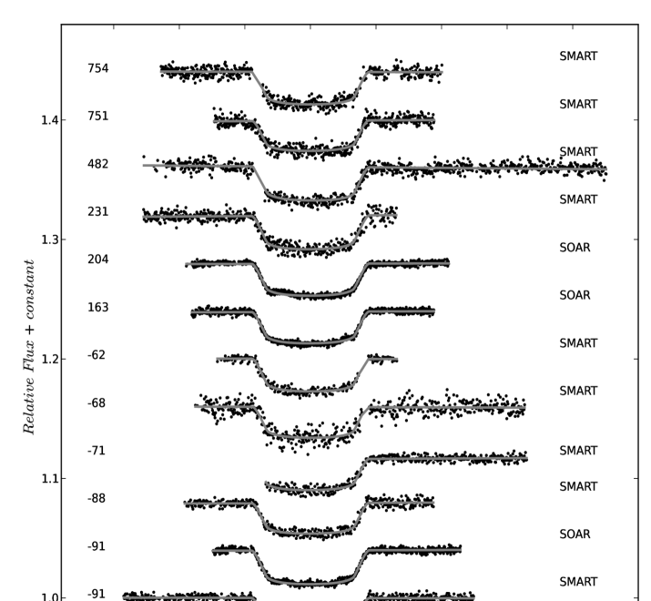
Figure 2: Light curves of the twelve new transits of WASP-4b presented in this work after the detrending described in Section 3. The solid lines show our best model fits using TAP. The epoch number is indicated to the left of each light curve and the telescope on the right.

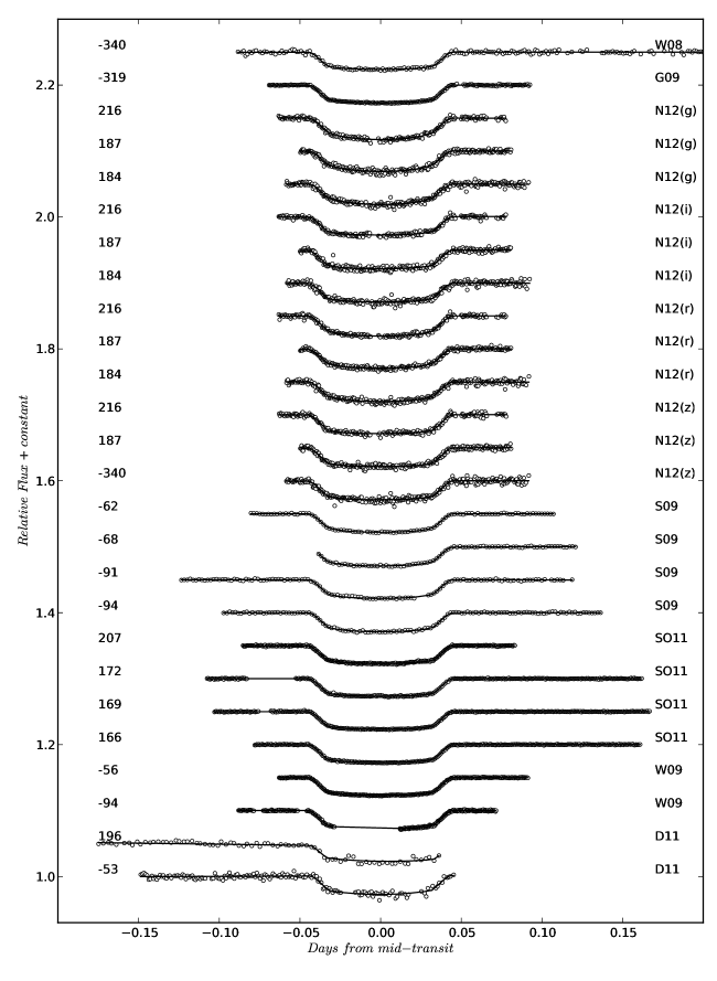
Figure 3: Light curves of the twenty-six transits of WASP-4b available in the literature. The solid lines show our best model fits using the TAP. The epoch is indicated on the left of each light curve. The author of each light curve is indicated on the righ.

We fitted the twelve new transit light curves presented in this work and the other 26 available light curves from W08, G09, W09, S09, D11, SO11 and N12. To perform the modelling we grouped all the light curves observed with the same filter in a given telescope (we treated all our light curves as observed with the same filter/telescope). As we described below, this allows us to fit for the linear limb-darkening coefficient ($\mu_{1}$) using all the light curves simultaneously as was done in Hoyer et al. (2012). Therefore, the first group is composed by our ten I-band light curves (from 2008 to 2010) and the second by our two Cousins-R light curves (the 2011’s transits). A third group is formed by the six SO11 z-band light curves (which includes the two transits observed by W09) and the S09 light curves form the fourth group (Cousins-R). We fit the V- and R-light curves of D11 separately. Finally, we fit the twelve light curves of N12 in four groups (three light curves for each of the four filters).

We fit each group independently, leaving as free parameters for each light curve the orbital inclination ($i$), the planet-to-star radius ratio ($R_{p}/R_{s}$) and the central time of the transit ($T_{c}$). The orbital period, the eccentricity, and the longitude of the periastron were fixed to the values $P=1.33823326~{}days$ (from D11), $e=0$ and $\omega=0$. We searched for possible linear trend residuals in the light curves by fitting for the out-of-transit flux ($F_{OOT}$) and for a flux slope ($F_{slope}$), but did not find any. The ratio between the semi-major axis and the star radius, $a/R_{s}$, usually presents strong correlations with $i$ and $R_{p}/R_{s}$. To break those correlations and their effects in our results (and because we are searching for relative variations in $i$ and $R_{p}/R_{s}$), we fixed $a/R_{s}$ in all the light curves to 5.53 (from D11). We checked that doing this we are not introducing any bias/effect on the rest of the parameters fitted and its errors (for details, see Hoyer et al. 2012). In particular we are not affecting the mid-times of the transits due to its weak correlation with $a/R_{s}$. We also fit for a white and red noise parameter, $\sigma_{w}$ and $\sigma_{r}$, respectively, as defined by Carter & Winn (2009).

The coefficients of a quadratic limb-darkening law ($\mu_{1}$ and $\mu_{2}$) in our light curves are strongly correlated, therefore we fixed $\mu_{2}$ to 0.32 (based in the tabulated values by Claret 2000) and let $\mu_{1}$ as free parameter on each group of light curves.

Therefore, for each light curve fit we obtained a value of $i$, $R_{p}/R_{s}$, $\sigma_{w}$, $\sigma_{r}$ and $T_{c}$ and a single value of $\mu_{1}$ for each group.

To fit the transits and derive errorbars for all parameters we ran 10 MCMC chains of $10^{5}$ links each, discarding the first 10% of the results from each chain to minimize any bias introduced by the parameter initial values. The resulting values for each parameter of the thirty-eight light curves together with their 1$\sigma$ errors are shown in Table 2 and 3. The data and the best models fits for all twelve light curves presented in this work are illustrated in Figure 2. The same is shown in Figure 3 for the twenty-six light curves from the literature.

Variations in transit parameters, in particular in $i$ and $R_{p}/R_{s}$, can be attributed to the perturbations produced by an additional body in the system. In Figure 4, we plot $R_{p}/R_{s}$ and $i$ as a function of the transit epoch, based in the results of the 38 transit fits. We do not find any significant variations in those parameters. As reference, in Figure 4 the weighted average values and the $\pm 1\sigma$ errors of $i$ and $R_{p}/R_{s}$ based on all the light curves results are represented by the solid and dashed horizontal lines, respectively. Our analysis of the transit timing is described in detail in section 5.

Is worthy to noticing that including the detrending parameters in the MCMC during the modelling is the most appropriate approach to estimate uncertainties of the transit parameters. We have checked that in our data there is no significant differences by doing the detrending before the MCMC fitting. The TAP version we use (v2.104) does not allow to detrend against airmass or X-Y position of the centroid or neither perform quadratic regression fits of the flux against the time, that is why we decided to check for correlations against these parameters before modelling with TAP. Also, most of the literature light curves we used to search for variations in transit parameters have been already detrended and therefore the uncertainties we estimate from them can be compared with those obtained from our data when we detrended it before the MCMC modelling.

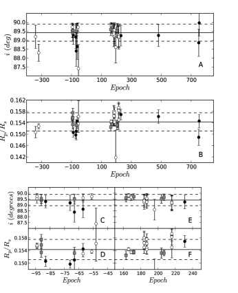
Figure 4: The orbital inclination (Panel A) and the planet-to-star radii ratio (Panel B) we derived for the twelve transit we present in this work (solid symbols) and for the twenty-six transits available in the literature (open symbols), as a function of the transit epoch. The parameters derived from transits with evidence of star-spot occultations are shown with gray squares. The solid and dashed horizontal lines represent the weighted average and its $\pm 1\sigma$ errors, respectively. There is no evidence of variations on these parameters for the time span of the observations. In the bottom panels we show a zoom of the diagrams around the -70th (Panel C and D) and 200th epochs (Panel E and F).

Table 2: Parameters derived for each of the twelves new transits of WASP-4b presented in this work. We modeled each light curve individually with TAP while $\mu_{1}$ was fitted simultaneously from light curves of the same filter.

Epoch	Filter	$T_{c}-2450000$	$i$	$R_{p}/R_{s}$	$\mu_{1}$	$\sigma_{red}^{a}$	$\sigma_{white}^{a}$	RMS	Spot
		($BJD_{TT}$)	$(\degr)$					(residuals)	Detectionb
-91	I	$4701.81280^{+0.00022}_{-0.00023}$	$89.52^{+0.33}_{-0.44}$	$0.1558^{+0.0012}_{-0.0012}$	$0.217^{+0.019}_{-0.020}$	$0.0066$	$0.0017$	$0.0023$	$\surd$
-91	”	$4701.81303^{+0.00018}_{-0.00019}$	$89.53^{+0.33}_{-0.44}$	$0.1575^{+0.0016}_{-0.0016}$	”	$0.0101$	$0.0012$	$0.0015$	$\surd$
-88	”	$4705.82715^{+0.00029}_{-0.00030}$	$89.29^{+0.48}_{-0.59}$	$0.1506^{+0.0016}_{-0.0017}$	”	$0.0066$	$0.0022$	$0.0024$	$\cdots$
-71	”	$4728.57767^{+0.00043}_{-0.00042}$	$89.18^{+0.57}_{-0.75}$	$0.1497^{+0.0013}_{-0.0013}$	”	$0.0046$	$0.0021$	$0.0023$	$\cdots$
-68	”	$4732.59197^{+0.00050}_{-0.00051}$	$88.39^{+0.96}_{-0.76}$	$0.1510^{+0.0031}_{-0.0030}$	”	$0.0165$	$0.0034$	$0.0049$	$\cdots$
-62	”	$4740.62125^{+0.00036}_{-0.00035}$	$88.64^{+0.82}_{-0.63}$	$0.1545^{+0.0018}_{-0.0017}$	”	$0.0058$	$0.0019$	$0.0021$	$\cdots$
163	”	$5041.72377^{+0.00019}_{-0.00018}$	$89.59^{+0.29}_{-0.40}$	$0.1525^{+0.0014}_{-0.0014}$	”	$0.0095$	$0.0012$	$0.0014$	$\surd$
204	”	$5096.59148^{+0.00023}_{-0.00022}$	$89.53^{+0.32}_{-0.45}$	$0.1533^{+0.0016}_{-0.0016}$	”	$0.0108$	$0.0022$	$0.0013$	$\surd$
231	”	$5132.72310^{+0.00041}_{-0.00041}$	$89.25^{+0.51}_{-0.66}$	$0.1569^{+0.0018}_{-0.0019}$	”	$0.0082$	$0.0021$	$0.0034$	$\cdots$
482	”	$5468.61943^{+0.00046}_{-0.00046}$	$89.26^{+0.52}_{-0.70}$	$0.1562^{+0.0023}_{-0.0025}$	”	$0.0166$	$0.0034$	$0.0033$	$\cdots$
751	R	$5828.60375^{+0.00042}_{-0.00041}$	$88.85^{+0.75}_{-0.78}$	$0.1489^{+0.0028}_{-0.0029}$	$0.212^{+0.066}_{-0.067}$	$0.0167$	$0.0021$	$0.0033$	$\cdots$
754	”	$5832.61815^{+0.00041}_{-0.00042}$	$88.96^{+0.69}_{-0.76}$	$0.1546^{+0.0024}_{-0.0023}$	”	$0.0141$	$0.0023$	$0.0033$	$\cdots$
a $\sigma_{red}$ and $\sigma_{white}$ parameters as defined by Carter & Winn (2009).
b Detections of spot-crossing events during transits ($\surd$: positive detection, $X$: negative detection, $\cdots$: inconclusive). See Section 6 for details.

Table 3: Parameters derived for each of the 26 transits of WASP-4b reanalized in this work. We modeled each light curve individually with TAP while $\mu_{1}$ was fitted simultaneously from light curves of the same filter of a given telescope.

Epoch	Authora,	$T_{c}-2450000$	$i$	$R_{p}/R_{s}$	$\mu_{1}$	$\sigma_{red}^{b}$	$\sigma_{white}^{b}$	RMS	Spot
	Filter	($BJD_{TT}$)	$(\degr)$					(residuals)	Detectionc
-340	W08, R	$4368.59279^{+0.00033}_{-0.00032}$	$89.19^{+0.57}_{-0.73}$	$0.1507^{+0.0020}_{-0.0020}$	$0.219^{+0.073}_{-0.078}$	$0.0036$	$0.0015$	$0.0016$	$\cdots$
-319	G09, z	$4396.69576^{+0.00012}_{-0.00012}$	$88.29^{+0.47}_{-0.49}$	$0.15279^{+0.00094}_{-0.00085}$	$0.253^{+0.030}_{-0.037}$	$0.0027$	$0.0005$	$0.0006$	$X$
-94	S09, R	$4697.79788^{+0.00013}_{-0.00013}$	$89.53^{+0.32}_{-0.41}$	$0.15533^{+0.00072}_{-0.00072}$	$0.333^{+0.017}_{-0.017}$	$0.0010$	$0.0006$	$0.0008$	$X$
-91	”	$4701.81234^{+0.00026}_{-0.00026}$	$89.41^{+0.41}_{-0.53}$	$0.1534^{+0.0016}_{-0.0015}$	”	$0.0037$	$0.0007$	$0.0008$	$\surd$
-68	”	$4732.59188^{+0.00027}_{-0.00027}$	$89.51^{+0.34}_{-0.49}$	$0.1532^{+0.0017}_{-0.0020}$	”	$0.0025$	$0.0005$	$0.0007$	$\surd$
-62	”	$4740.62118^{+0.00016}_{-0.00016}$	$89.59^{+0.29}_{-0.41}$	$0.1530^{+0.0010}_{-0.0011}$	”	$0.0020$	$0.0005$	$0.0006$	$X$
-94	W09, z	$4697.79817^{+0.00008}_{-0.00009}$	$89.73^{+0.19}_{-0.28}$	$0.15560^{+0.00077}_{-0.00079}$	$0.2027^{+0.0076}_{-0.0076}$	$0.0027$	$0.0005$	$0.0007$	$\cdots$
-56	”	$4748.65111^{+0.00007}_{-0.00007}$	$89.72^{+0.20}_{-0.28}$	$0.15369^{+0.00057}_{-0.00058}$	”	$0.0024$	$0.0003$	$0.0005$	$X$
-53	D11, V	$4752.66576^{+0.00067}_{-0.00069}$	$87.4^{+1.6}_{-1.1}$	$0.1562^{+0.0053}_{-0.0059}$	$0.50^{+0.18}_{-0.16}$	$0.0104$	$0.0022$	$0.0029$	$\cdots$
196	D11, R	$5085.88418^{+0.00084}_{-0.00086}$	$88.6^{+0.79}_{-0.99}$	$0.1418^{+0.0092}_{-0.0099}$	$0.42^{+0.20}_{-0.19}$	$0.0132$	$0.0012$	$0.0026$	$\cdots$
166	SO11, z	$5045.73853^{+0.00008}_{-0.00008}$	$89.8^{+0.14}_{-0.22}$	$0.15441^{+0.00053}_{-0.00055}$	$0.2027^{+0.0076}_{-0.0076}$	$0.0023$	$0.0004$	$0.0005$	$X$
169	”	$5049.75325^{+0.00007}_{-0.00007}$	$89.65^{+0.24}_{-0.29}$	$0.15347^{+0.00049}_{-0.00047}$	”	$0.0018$	$0.0004$	$0.0005$	$X$
172	”	$5053.76774^{+0.00009}_{-0.00009}$	$89.72^{+0.19}_{-0.28}$	$0.15346^{+0.00058}_{-0.00058}$	”	$0.0026$	$0.0004$	$0.0005$	$\surd$
207	”	$5100.60595^{+0.00012}_{-0.00012}$	$89.66^{+0.23}_{-0.32}$	$0.15318^{+0.00086}_{-0.00087}$	”	$0.0043$	$0.0004$	$0.0007$	$\surd$
184	N12, g’	$5069.82676^{+0.00031}_{-0.00030}$	$89.22^{+0.54}_{-0.64}$	$0.1550^{+0.0019}_{-0.0020}$	$0.598^{+0.029}_{-0.031}$	$0.0061$	$0.0020$	$0.0026$	$\cdots$
187	”	$5073.84108^{+0.00028}_{-0.00029}$	$89.34^{+0.47}_{-0.57}$	$0.1548^{+0.0020}_{-0.0020}$	”	$0.0056$	$0.0017$	$0.0023$	$\cdots$
216	”	$5112.65009^{+0.00032}_{-0.00033}$	$89.13^{+0.58}_{-0.68}$	$0.1593^{+0.0020}_{-0.0020}$	”	$0.0001$	$0.0015$	$0.0018$	$\cdots$
184	N12, i’	$5069.82617^{+0.00038}_{-0.00038}$	$89.42^{+0.41}_{-0.60}$	$0.1574^{+0.0026}_{-0.0029}$	$0.238^{+0.037}_{-0.040}$	$0.0$	$0.0021$	$0.0028$	$\cdots$
187	”	$5073.84128^{+0.00025}_{-0.00026}$	$89.52^{+0.34}_{-0.58}$	$0.1562^{+0.0019}_{-0.0019}$	”	$0.0$	$0.0018$	$0.0025$	$\cdots$
216	”	$5112.65005^{+0.00048}_{-0.00049}$	$89.25^{+0.52}_{-0.70}$	$0.1550^{+0.0034}_{-0.0033}$	”	$0.0020$	$0.0008$	$0.0019$	$\cdots$
184	N12, z’	$5069.82670^{+0.00028}_{-0.00027}$	$89.41^{+0.42}_{-0.55}$	$0.1580^{+0.0018}_{-0.0018}$	$0.218^{+0.034}_{-0.035}$	$0.0$	$0.0023$	$0.0029$	$\cdots$
187	”	$5073.84111^{+0.00023}_{-0.00023}$	$89.25^{+0.51}_{-0.58}$	$0.1576^{+0.0017}_{-0.0017}$	”	$0.0$	$0.0016$	$0.0022$	$\cdots$
216	”	$5112.64986^{+0.00036}_{-0.00039}$	$89.18^{+0.56}_{-0.68}$	$0.1583^{+0.0025}_{-0.0025}$	”	$0.0$	$0.0016$	$0.0020$	$\cdots$
184	N12, r’	$5069.82661^{+0.00029}_{-0.00029}$	$89.34^{+0.46}_{-0.59}$	$0.1564^{+0.0019}_{-0.0020}$	$0.390^{+0.025}_{-0.027}$	$0.0003$	$0.0019$	$0.0025$	$\cdots$
187	”	$5073.84114^{+0.00018}_{-0.00018}$	$89.56^{+0.30}_{-0.44}$	$0.1543^{+0.0013}_{-0.0014}$	”	$0.0002$	$0.0011$	$0.0017$	$\cdots$
216	”	$5112.65005^{+0.00031}_{-0.00031}$	$89.20^{+0.55}_{-0.67}$	$0.1587^{+0.0019}_{-0.0019}$	”	$0.0$	$0.0014$	$0.0018$	$\cdots$
a Transits from W08 (Wilson et al., 2008), G09 (Gillon et al., 2009), S09 (Southworth et al., 2009), W09 (Winn et al., 2009), D11 (Dragomir et al., 2011),
SO11 (Sanchis-Ojeda et al., 2011) and N12 (Nikolov et al., 2012).
b $\sigma_{red}$ and $\sigma_{white}$ parameters as defined by Carter & Winn (2009).
c Detections of spot-crossing events during transits ($\surd$: positive detection, $X$: negative detection, $\cdots$: inconclusive). See Section 6 for details.

4.2 Global Analysis

Since we find no evidence of significant variations in the parameters fitted for each individual light curve, we can model all light curves simultaneously to improve the determination of $i$, $R_{p}/R_{s}$ and $a/R_{s}$. For this, we fitted simulaneausly these parameters in the 38 light curves, while letting to vary on each light curve the transit mid-times, $F_{slope}$, $F_{OOT}$, $\sigma_{W}$ and $\sigma_{red}$. We fixed P and the linear and quadratic limb-darkening coefficients for each filter to the values obtained in the previous section. We used 10 chains of $10^{5}$ links each in the MCMC. The resulting values of the MCMC analysis for the simultaneuosly fitted parameters are shown in Table 4 and the resulting distributions in Figure 5. Using the resulting value for $R_{p}/R_{s}$ and the value of the star radius ($R_{S}=0.907\pm 0.014~{}R_{\sun}$) derived by SO11, we obtained an improved radius measurement for the planet of $R_{p}=1.395\pm 0.022~{}R_{jup}$, which is consistent with the most recent radius estimation reported by SO11 and N12.

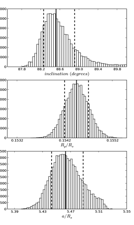
Figure 5: Distributions of the MCMC results of the 10 chains of $10^{5}$ links each obtained by fitting simultaneously the orbital inclination, $R_{p}/R_{s}$ and $a/R_{s}$ in the 38 available light curves of WASP-4.

5 Timing analysis and limits to additional planets

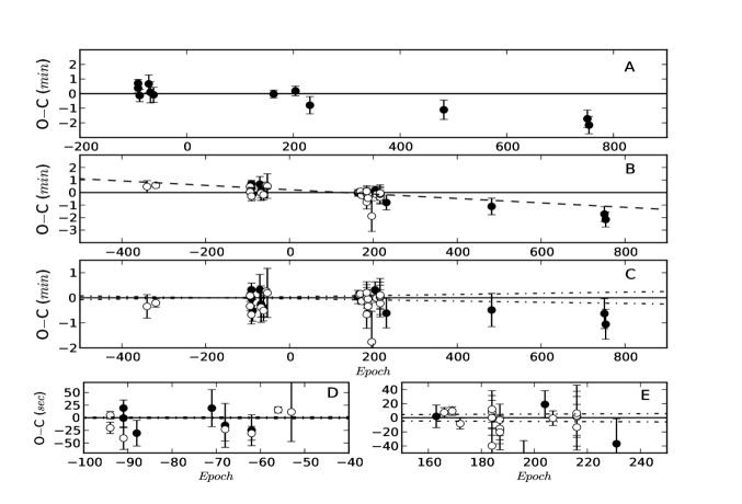
Figure 6: $Observed$ $minus$ $Calculated$ diagrams of the WASP-4b’s transits. Panel A: Timing residuals of the observed new twelve transit midtimes presented in this work compared with the predicted ephemerides from D11. Panel B: Our twelve $T_{c}$ (solid circles) combined with the new times derived from W08, G09, W09, S09, SO11, D11 and N12 (open circles). A linear trend in the residuals is evident. Panel C: If the linear trend is removed, with the updated ephemeris equation (shown by the horizontal solid line) the $RMS$ of the timing residuals is $20$ seconds. The $\pm 1\sigma$ levels are shown by the point-dashed lines. Panel D and E: we show a close view centered in -70 and 200 epoch, respectively. The lines are as in Panel C. An excellent agreement is found in the mid-times derived from the common epoch transits and with the updated ephemeris equation.

The times of our twelve transits and the D11 transits were initially computed in Coordinated Universal Time (UTC) and then converted to Barycentric Julian Days, expressed in Terrestrial Time, BJD(TT), using the Eastman et al. (2010) online calculator. The time stamps of the S09 light curves were initially expressed in HJD(UT) and have also been converted to BJD(TT). The same was done with the transit midtimes obtained from W08 and G09 light curves. No conversion was necessary for the light curves reported by SO11 (which includes the two transits of W09) and the ones reported by N12, since they are already expressed in BJD(TT). Finally, we did not include the $T_{c}$ derived from the 2006 and 2007 WASP data since that value is based on the folded transits of the entire WASP observational seasons, and therefore lacks the precision required for our timing analysis.

We used the D11 ephemeris equation to calculate the residuals of the mid-times of the 38 transits of WASP-4b analyzed in this work. Panel A in Figure 6 shows the $Observed$ $minus$ $Calculated$ ($O-C$) diagram of the times for our twelve transits. In panel B we combined the $O-C$ values of these twelve transits with the new values derived for the W08, G09, W09, S09, SO11, D11 and N12 (shown as open circles). A linear trend is evident in the residuals of all the transits (represented by a dashed line in panel B). That trend is caused by the accumulated error over time in the transit ephemerides. Once those ephemerides are updated, that trend is removed (panel C), and the RMS of the transit times residuals is only of $29$ seconds. The reduced-chi-squared of the linear regression is $\chi^{2}_{red}=1.25$ ($\chi^{2}=45$ for 36 degrees of freedom). If we removed the D11’s transit with the largest uncertainties (E=196, which corresponds to an incomplete transit observation) and re-calculated the linear trend, the RMS of the residuals is only $20$ seconds after updated the ephemerides ($\chi^{2}_{red}=1.18$, $\chi^{2}=41.3$ for 35 degrees of freedom).

Once the linear trend is removed (using the linear regression with $\chi^{2}_{red}=1.18$) the updated ephemeris equation is:

$$T_{c}=2454823.591924(28)[BJD_{TT}]+1.33823204(16)\times E,$$ (1)

where $T_{c}$ is the central time of a transit in the epoch $E$ since the reference time $T_{0}$. The errors of the last digits are shown in parenthesis.

Panel C in Figure 6 shows the resulting $O-C$ values of all available transits using the updated ephemeris equation. Almost all the $T_{c}$ coincide with it within the $\pm 1~{}\sigma$ errors represented by the point-dashed lines. Despite there is still non negligible residuals in the timing of $E=751,754$ transits (panel C) those epochs do not deviate from the updated ephemeris equation by more than $2.5\sigma$. These points have relative large uncertainties compare with other epochs and therefore have less weight in the calculated linear regression. We found no evidence of a quadratic function in the $O-C$ values. We show in panels D and E a close-up of the $O-C$ diagram around the -70 and 200 epochs, were the transit observations are more clustered. All the $T_{c}$ of the common transits analyzed in this work are in excellent agreement within the errors.

This newly obtained precision permits to place strong constraints in the mass of an hypothetical companion, particularly in MMR’s, as we discuss below.

We used the Mercury N-body simulator (Chambers, 1999) to place upper limits to the mass of a potential perturber in the WASP-4 system, based on our timing analysis of the transits. A detailed description of the setup we used for running the dynamical simulations can be found in Hoyer et al. (2011) and Hoyer et al. (2012). As a summary, for the simulated perturber bodies we used circular ($e=0$) and coplanar orbits with WASP-4b. We explored a wide range of perturber masses ($0.1M_{\earth}~{}\leq M_{pert}\leq 5000M_{\earth}$) and distances between $0.1~{}AU$ and $0.06~{}AU$ in steps of $0.001~{}AU$. The semi-major axis steps were reduced to $0.0005~{}AU$ near MMRs with the respective transiting body. The density of the perturber body corresponds to the mean density of the Earth (for $M_{pert}\leq 1M_{\earth}$) or Jupiter (for $\geq 300M_{\earth}$). The density was obtained from a linear function that varies from Earth’s to Jupiter’s density for all the other $M_{pert}$.

We identified a region of unstable orbits where any orbital companion experimented close encounters with the transiting body in the time of the integrations we studied (10 years). For all the other stable orbits we recorded the central times of the transits, which were compared with predicted times assuming an average constant orbital period for each system. This period did not deviate by more than $3\sigma$ from the derived period of each transiting body. When the calculated TTV RMS approached to 60 seconds we reduced the mass sampling in order to obtain high precision values ($\leq 1~{}M_{\earth}$) in the mass of the perturber.

The results of our model simulations are illustrated in Figure 7, where we show the perturber mass, $M_{pert}$ ($M_{\earth}$), versus orbital semi-major axis, $a$ ($AU$), diagram that places the mass limits to potential perturbers in the system. The solid line in the diagram indicates the derived upper limits to the mass of the perturbers that would produce TTV RMS of $20$ seconds at different orbital separation. The dashed line shows the perturber mass upper limits imposed by the most recent RV observations of the WASP-4 system, for which we have adopted a precision of $15~{}m~{}s^{-1}$ (Triaud et al., 2010).

In the same figure, we also show the result of calculating the MEGNO (Mean Exponential Growth of Nearby Orbits) factor $\langle Y\rangle$ (Cincotta & Simó, 1999, 2000; Cincotta et al., 2003) which measures the degree of chaotic dynamics of the potential perturber. This technique found widespread application within dynamical astronomy in studies of stability and orbital evolution, in particular in extrasolar planetary systems and Solar system bodies (Goździewski et al., 2001; Goździewski & Maciejewski, 2001; Hinse et al., 2010). Here we use MEGNO to identity phase space regions of orbital instability in the WASP-4 system. We calculated $\langle Y\rangle$ on a grid considering 450x400 initial conditions with the perturber initially placed on a $e=0$ orbit in all integrations. The transiting planet is located at $a=0.02312~{}AU$ from the host star. Each test orbit was integrated for $10^{6}$ days. For quasi-periodic orbits $\langle Y\rangle\rightarrow 2.0$ for $t\rightarrow\infty$ and for chaotic orbits $\langle Y\rangle\neq 2$ (represented by the gray region in the figure). In theses cases $\langle Y\rangle$ usually diverges quickly away from 2.0 in the beginning of the orbit integration. The region close to the transiting planets is highly chaotic due to strong gravitational interactions resulting in collisions and/or escape scenarios and coincides with the unstable region we have identified with Mercury code. We identify the locations of MMRs by the chaotic time evolution at certain distances from the host star. These coincide with the TTV sensitivity for smaller masses of the perturber.

For WASP-4b, we found that the upper limits in the mass of an unseen orbital companion are 2.5, 2.0 and 1.0 $M_{\earth}$ in the 1:2, 5:3 and 2:1 MMRs respectively (vertical lines in Figure 7). These limits are more strict than the radial velocities constraints, specially in the MMRs, although by using our approach we can not reproduce the mass limits derived by N12.

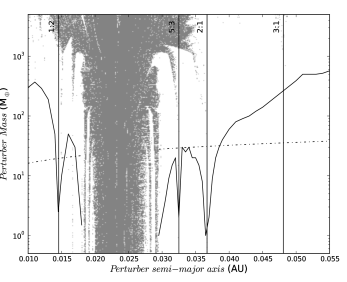
Figure 7: Upper mass limits as function of the orbital semi-major axis of an hypothetical perturber of the exoplanet WASP-4b, based on dynamical simulations done with the Mercury N-body simulator (Chambers et al. 1999). The solid line corresponds to perturber masses which produce TTVs RMS of $\sim 20$ as we measure in our timing analysis (see section 5). The point-dashed line shows the limits imposed by the radial velocity measurements. Vertical lines mark the locations of MMRs with WASP-4b and the gray region indicates MEGNO factor $\langle Y\rangle\neq 2$, i.e. the region of chaotic orbits in the system.

6 Starspot Occultations

Table 4: New derived parameters for the WASP-4 system using the results of the simultaneous modelling of all available light curves (Section 4.2). The orbital period, P, and the reference epoch, $T_{0}$, were determined in the timing analysis of the transits (Section 5).

Parameter	Derived Value	error
P ($days$)	$1.33823204$	$\pm 0.00000016$
$T_{0}$ ($BJD_{TT}$)	$2454823.591924$	$\pm 0.000028$
$i$ (deg)	$88.52$	$+0.39,-0.26$
$R_{p}/R_{s}$	$0.15445$	$\pm 0.00025$
$a/R_{s}$	$5.463$	$+0.025,-0.020$
$R_{p}$ ($R_{jup}$)	$1.395$	$\pm 0.022$
$e$	$0$ a	$\cdots$
a This value was fixed in the light curve modelling.

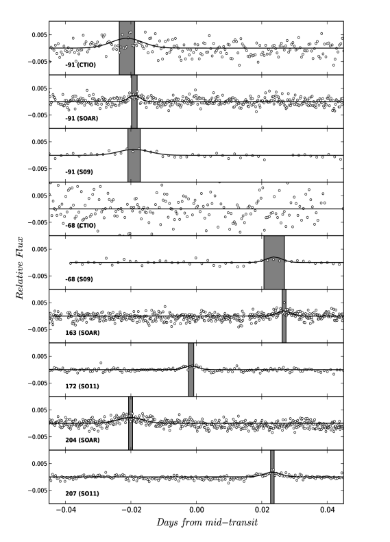
Figure 8: Light curves with evidences of star-spot occultations by WASP-4b are shown. The epoch and telescope (or the author) of the light curve are shown in the bottom left. The solid lines represent the fitted gaussian model and the gray regions are proportional to the uncertainties in the timing of the occultations. We confirm the detection of the occultation with our -91 epoch’s data but in our -68 transit we found no evidence of occultation due the low SNR of the data.

Table 5: Results of the fitting of the star-spots occultations. For each light curve, the amplitude ($A_{occ}$), the central time of the occultation ($T_{occ}$) relative to midtime of the transit ($T_{c}$) and the width of the fitted Gaussian function ($\sigma$) are shown. The errors were obtained from Monte-Carlo

Epoch	RMS	$A_{occ}$  (ppm)	$T_{c}-T_{occ}$ (days)	$\sigma$ (days)
-91 (CTIO)	0.0023	$0.0037\pm 0.0037$	$-0.0211\pm 0.0023$	$0.0048\pm 0.0027$
-91 (SOAR)	0.0015	$0.0024\pm 0.0006$	$-0.0189\pm 0.0008$	$0.0018\pm 0.0009$
-91 (S09)	0.0008	$0.0022\pm 0.0006$	$-0.0190\pm 0.0019$	$0.0047\pm 0.0018$
-68 (S09)	0.0007	$0.0021\pm 0.0020$	$0.024\pm 0.003$	$0.0024\pm 0.0019$
163 (SOAR)	0.0014	$0.0019\pm 0.0003$	$0.0268\pm 0.0006$	$0.0022\pm 0.0008$
172 (SO11)	0.0005	$0.0014\pm 0.0004$	$-0.0016\pm 0.0008$	$0.0021\pm 0.0006$
204 (SOAR)	0.0014	$0.0022\pm 0.0003$	$-0.0201\pm 0.0006$	$0.0039\pm 0.0006$
207 (S011)	0.0007	$0.0017\pm 0.0007$	$0.0232\pm 0.0005$	$0.0026\pm 0.0009$

As SO11 previously noted, in some of the light curves during the transit there are bump-like features or anomalies that can be interpreted as star-spot occultations by the exoplanet while it crosses in front the star’s disk. SO11 detected evidence of these occultations in two of the light curves they presented and in the two light curves of S09. Depending on the SNR and the sampling of the data, we also identified these bumps in four of our light curves (during three different epochs).

Using the residuals of the detrended light curves after modelling the transits (see section 4), we fit a gaussian function around each bump feature, initially identified by eye and which we assume are caused by spots. In particular we fit for the amplitude ($A_{occ}$), central time of the spot occultation ($T_{occ}$) and the width ($\sigma$) of the Gaussian which can be used to described the duration of the occultation event. To estimate the uncertainties of these values, before fitting we added to the observational points an amount of random noise proportional to the RMS of the residuals (without bumps). We repeated this procedure 10 000 times for each light curve and calculated the errors from the width of the resulting distributions. In Figure 8 we show the results of those fits for the light curves that present signs of spots in the stars. No spots were apparent in the remaining light curves. Our data of the -91 transit epoch confirms the detection of a spot occultation in the S09 light curve by SO11. Given the better sampling and signal-to-noise ratio (SNR) of our SOAR light curve, we can improve the central timing of the spot by a factor of three, as illustrated by the gray vertical bands in Figure 8, which indicate the error obtained in the central timings of each spots. However, our CTIO light curve of the transit epoch -68 shows no sign of spots and we cannot confirm the spot in that epoch in the S09 light curve. This can be attributed to the worse SNR of our light curve, but notice also that the amplitude of the spot occultation that we obtain in the S09 data is $A_{occ}=0.0021\pm 0.0020$. Therefore that detection could render spurious. Among our new data we also detect two new spots during transit epochs 163 and 204.

In Table 5 we show the results of the gaussian fits. Taking into account the values obtained for $A_{occ}$ and the RMS values of the residuals, no starspot occultations were detected in the light curves of the epochs: -88, -71, 166 and 169. These non-detections (especially the transits closer to those with positive detections) can be used to constrain the spot’s location and/or lifetime. For example, it can be argued that during those transits the spot is located in the non-visible hemisphere of the star, or that the spot have migrated to different latitudes that those occulted by the exoplanet’s path.

SO11 found two possible values for the rotation period of the star, $22.2~{}days$ (based on the spots of their new light curves), and $25.5~{}days$, based on the S09 light curves. Both results are consistent with the constraint of the radial velocities measurements (Triaud et al., 2010).

We used a simple linear model to estimate the rotational period of WASP-4 relying only in the timing of the occultations. We assumed an aligned system (an assumption consistent with the RM effect observations and with the SO11’s previous analysis of the spots) since this geometry increases the probability of detecting occultations of the same spots by the exoplanet.

We assigned angular coordinates for the location of the spots, such that at ingress (first contact) and at egress (fourth contact) of the transit a spot will have a relative angle of $0\degr$ and $180\degr$, respectively. Relative angles in the non-visible hemisphere will extent between $180\degr$ and $360\degr$. For the epochs where no spot occultations were detected we assigned an aleatory angle for the location of the spot between 180 and 360 degrees and assumed larger errors in its timing ($\sim 0.05~{}days$) to compensate for the non-detection during transit. Later, as explained below, we checked if the rotational period we obtained is consistent with the corresponding non-detections.

Then, we fit the following linear function for the displacement of the spots:

$$\delta\Theta=\Theta_{0}+\Omega\cdot(T-T_{0}),$$ (2)

where $\Theta_{0}$ is the relative angle of the spot in an arbitrary reference time $T_{0}$, and $\Omega$ is the displacement rate of the spots due to stellar rotation (assuming no migration), in degrees per days. To test our model we fit the same spot pairs analyzed by SO11 (E=172,207), using our newly computed $T_{occ}$ and obtain a stellar rotation period $P_{rot}=22.7\pm 0.2~{}days$, consistent with the $22.2~{}days$ period derived by SO11 but inconsistent with the non-detections of E=166,169. Our new occultation central times for the S09 spots (E=-91,-68) give a $P_{rot}$ of $27.5\pm 0.5~{}days$, slightly longer than the $25.5~{}days$ period obtained by SO11 but consistent with the no-detections in E=-62,-56. We conclude that, to first order approximation, our linear model provides a good estimate of the star’s rotational period, given the available data.

Next we tried to improve the $P_{rot}$ of the star by adding, first, the new 204 transit epoch to the 172 and 207 epochs (we assumed the spot was the same in the 47 days covered by those epochs). The first minimum of the fit to those three epochs gives a $P_{rot}$ of $44\pm 1~{}days$ ($\chi^{2}=10^{2}$). That period is almost twice the value derived by SO11 and their value of the RV constraints estimated to be $\sim(21.5\pm 4.3~{}days)\times sin(i_{s})$, where $i_{s}$ is the inclination of the stellar rotation axis with respect to the line of sight. The second minimum of the fit gives a $P_{rot}$ of $22.4\pm 0.2~{}days$ but with a $\chi^{2}\sim 10^{3}$. This high values of the $\chi^{2}$ mean that none of the obtained values of $P_{rot}$ are consistent with the the locations of the spot in the three epochs. Both solutions deviate by more than $10\degr$ in the location of the spot in E=204 event. The second minimun is also inconsistent with the location of the spot in E=207 while the first minimum is consistent with it within the errors. Furthemore, these solutions are inconsistent with the no-detection of the spot during E=166,169. Probably this is an indication that the events occurring in the 172 and 204-207 epoch do not correspond to occultations of same star-spot and therefore this is a constraint for the lifetime of the spot. Using only the spot $T_{occ}$ of the 204 and 207 epochs we obtained a $P_{rot}$ of $34\pm 2~{}days$. However, this period do not match the occultation of the 172 epoch event, supporting the idea that the occultations in E=172 and E=204,207 are over different spots ($\sim 43~{}days$ have elapse between the E=204 and E=172 transits). Nevertheless, is very likely that WASP-4b have occulted the same spot in E=204,207 due to time span between this events is only of $\sim 4~{}days$.

To explain why the $P_{rot}=34~{}days$ is above the limits of the RV’s measurements we can use the observed decrease in the amplitude and duration of spots between the 204 and 207 epochs. One possibility is that we are evidencing a change in the rotational speed of the spots over the average rotation of the star. The spot can be migrating to higher latitudes in the star surface, decreasing by this way the projected area that is being occulted by the planet, and if WASP-4 presents differential rotation (like the observed in the Sun), the relative displacement rate of the spot over the stellar surface could vary. Therefore the increment in the rotation period we observed compared with the values of the RV’s constraints and the rotational period we estimated using -91 and -68 data, can be indicative of the spot migration to latitudes with lower rotational periods. To fully support this argument we would need a more dense sample of transit observations using the same filters and observing configurations. A summary of the results of this section is presented in Table 6.

With the same analysis, if we fit the 163 and 172 epoch’s occultations, the minimum we found corresponds to a rotational period of $\sim 13\pm 0.2~{}days$ (also consistent with the no-detections of the 166 and 169 epochs) but again this period is far below the range indicated by the RV’s measurements and is a evidence that those occultation events are over different spots.

Of course, a more detailed model is necessary to constrain strictly the rotation period of the star. This model has to take into account other parameters such the amplitude and duration of the spot occultations, the relative angle between spin axis of the star axis and the orbital axis of the planet, the lifetime of the spots, etc.

Table 6: Results of the fitting of the rotational period of WASP-4 using different spot occultation events (indicated with bold numbers) and no-detection of occultations during transit. As reference, in the second column we indicate the time span between the first and last epoch used in the minimization. In the last column is indicated if the fitted $P_{rot}$ is consistent with the no-detections (No-D).

Epochs	time span	$P_{rot}$	$\chi^{2}$	No-D?
	$(days)$	$(days)$
166, 169, 172, 207	55	$22.7\pm 0.2$	$10^{-5}$	no
-91, -68 , -62, -56	47	$27.5\pm 0.5$	$10^{-7}$	yes
166, 169,172, 204, 207	55	$44\pm 1$	$10^{2}$	no
166, 169,172, 204, 207	55	$22\pm 0.4$	$10^{3}$	no
204, 207	4	$34\pm 1$	$10^{-8}$	$\cdots$
163, 166, 169, 172	12	$13\pm 0.2$	$10^{-8}$	yes

7 Summary

We present twelve new transit epoch observations of the WASP-4b exoplanet. These new transits observed by the TraMoS project were combined with all the light curves available in the literature for this exoplanet. It is worth noticing that the analysis and modelling we perform in Section 4 was done over detrended light curves (both for the TraMoS and literature data). This does not significantly affect the results in this paper because the system does not show TTVs. However, the light curve analysis should be done, whenever possible, including detrending coefficients as part of a global parameter fit. Therefore, we encourage authors to provide the raw light curves data in the publications to allow future homogeneous analyses of different datasets of a given planet. With an homogeneous modelling of all this data (the new presented here and the previously published) we performed a timing analysis of the transits. Based in the RMS of the $O-C$ diagram of about $20$ seconds we confirmed that WASP-4b orbits its host star with a linear orbital period. We updated the ephemeris equation of this planet and also refined the values of the inclination of the orbit and the planet-to-star radii ratio. Also, during the transits we detected small anomalies in the relative flux of four of the transits (of three different epochs) presented in this work. As Sanchis-Ojeda et al. (2011) previously noted we identified these anomalies as stellar spot occultations by the planet. With a simple modelling using the timing of these occultations we estimated the rotational period of the star. With the timing of the events we are more confident correspond to occultations of a same spot allowed to propose the rotational period is about 34 days. Since this value deviates from the limits imposed by the radial velocities measurements a further modelling that include spot migration and star differential rotation is needed. A monitoring of more consecutive transits will be necessary to allow for new spots detections and to do a better constrain in the rotational period of WASP-4. High cadence light curves with relative small dispersion are critical on this matter, as can be seen in our SOAR light curves.

8 Acknowledgements

The authors would like thank D. Dragomir and S. Kane for providing TERMS light curves, M. Gillon for the VLT data and the anonymous referee for the useful and accurate comments which helped to improve this manuscript. S.H. and P.R. acknowledge support from Basal PFB06, Fondap #15010003, and Fondecyt #11080271 and #1120299. S.H, received support from ALMA-CONICYT FUND #31090030 and from the Spanish Ministry of Economy and Competitiveness (MINECO) under the 2011 Severo Ochoa Excellence Program MINECO SEV-2011-0187 at the IAC. TCH acknowledges support from KRCF via the KRCF Young Scientist Fellowship program and financial support from KASI grant number 2013-9-400-00. TCH wish to acknowledge the SFI/HEA Irish Centre for High-End Computing (ICHEC) for the provision of computational facilities and support. V.N. acknowledge partial support by the Università di Padova through the ”progetto di Ateneo” #CPDA103591. We thanks the staff of CTIO and SOAR for the help and continuous support during the numerous observing nights, and R. Sanchis-Ojeda for helpful comments and discussions. Based on observations made with the SMARTS 1-m telescope at CTIO and the SOAR Telescope at Cerro Pachon Observatory under programmes ID CNTAC-08B-046,-09A-089,-09B-050,-10A-089 and -10B-066.

References

- Agol et al. (2005) Agol E., Steffen J., Sari R., Clarkson W., 2005, MNRAS, 359, 567
- Carter & Winn (2009) Carter J. A., Winn J. N., 2009, ApJ, 704, 51
- Chambers (1999) Chambers J. E., 1999, MNRAS, 304, 793
- Cincotta et al. (2003) Cincotta P., Giordano C., Simó C., 2003, Physica D, 182, 151
- Cincotta & Simó (1999) Cincotta P., Simó C., 1999, CMDA, 73, 195
- Cincotta & Simó (2000) Cincotta P., Simó C., 2000, ApJS, 147, 205
- Claret (2000) Claret A., 2000, A&A, 363, 1081
- Dragomir et al. (2011) Dragomir D. et al., 2011, AJ, 115
- Eastman et al. (2010) Eastman J., Siverd R., Gaudi B. S., 2010, PASP, 122, 935
- Gazak et al. (2011) Gazak J. Z., Johnson J. A., Tonry J., Eastman J., Mann A. W., Agol E., 2011, ArXiv e-prints
- Gillon et al. (2009) Gillon M. et al., 2009, A&A, 496, 259
- Goździewski et al. (2001) Goździewski K., Bois E., Maciejewski A. J., Kiseleva-Eggleton L., 2001, aap, 378, 569
- Goździewski & Maciejewski (2001) Goździewski K., Maciejewski A. J., 2001, apjl, 563, L81
- Hinse et al. (2010) Hinse T. C., Christou A. A., Alvarellos J. L. A., Goździewski K., 2010, mnras, 404, 837
- Holman & Murray (2005) Holman M. J., Murray N. W., 2005, Science, 307, 1288
- Hoyer et al. (2012) Hoyer S., Rojo P., López-Morales M., 2012, ApJ, 748, 22
- Hoyer et al. (2011) Hoyer S., Rojo P., López-Morales M., Díaz R. F., Chambers J., Minniti D., 2011, ApJ, 733, 53
- Kipping (2009) Kipping D. M., 2009, MNRAS, 392, 181
- Mandel & Agol (2002) Mandel K., Agol E., 2002, ApJL, 580, L171
- Mayor & Queloz (1995) Mayor M., Queloz D., 1995, Nature, 378, 355
- Miralda-Escudé (2002) Miralda-Escudé J., 2002, ApJ, 564, 1019
- Nikolov et al. (2012) Nikolov N., Henning T., Koppenhoefer J., Lendl M., Maciejewski G., Greiner J., 2012, A&A, 539, A159
- Sanchis-Ojeda et al. (2011) Sanchis-Ojeda R., Winn J. N., Holman M. J., Carter J. A., Osip D. J., Fuentes C. I., 2011, ApJ, 733, 127
- Silva-Valio (2008) Silva-Valio A., 2008, ApJL, 683, L179
- Southworth et al. (2009) Southworth J. et al., 2009, MNRAS, 399, 287
- Triaud et al. (2010) Triaud A. H. M. J. et al., 2010, A&A, 524, A25+
- Wilson et al. (2008) Wilson D. M. et al., 2008, ApJL, 675, L113
- Winn et al. (2009) Winn J. N., Holman M. J., Carter J. A., Torres G., Osip D. J., Beatty T., 2009, AJ, 137, 3826