Peixoto’s Structural Stability Theorem:
The One-dimensional Version

Abstract

Peixoto’s structural stability and density theorems represent milestones in the modern theory of dynamical systems and their applications. Despite the importance of these theorems, they are often treated rather superficially, if at all, in upper level undergraduate courses on dynamical systems or differential equations. This is mainly because of the depth and length of the proofs. In this note/module, we formulate and prove the one-dimensional analogs of Peixoto’s theorems in an intuitive and fairly simple way using only concepts and results that for the most part should be familiar to upper level undergraduate students in the mathematical sciences or related fields. The intention is to provide students who may be interested in further study in dynamical systems with an accessible one-dimensional treatment of structural stability theory that should help make Peixoto’s theorems and their more recent generalizations easier to appreciate and understand.

1 Introduction

Inspired by the pioneering work of [1] and encouraged by Solomon Lefschetz, the Brazilian engineer and mathematician, Maurício Matos Peixoto, formulated and proved the first global characterization of structural stability and its density properties on smooth surfaces [5] in terms that have become synonymous with the modern theory of dynamical systems and blazed a path for myriad extensions and generalizations. One of the most powerful aspects of Peixoto’s theorems is the way it uses local properties to characterize global features of dynamical systems. Both the structural stability and density theorems can be combined as follows (see Perko, etc.):

Theorem P (Peixoto’s Structural Stability and Density Theorems). Let $\dot{x}=f(x)$ be a $C^{1}$ dynamical system on a smooth closed surface $M$. Then the dynamical system is $C^{1}$-structurally stable if and only if it satisfies the following properties:

• All recurrent behavior is confined to finitely many fixed points and periodic orbits, all of which are hyperbolic.

• There are no separatrices, i.e. orbits connecting saddle points.

Moreover, if $M$ is orientable, then the set of structurally stable systems is $C^{1}$ open and dense in the collection of all dynamical systems on the surface.

This theorem involves mathematical concepts unfamiliar to many advanced undergraduates interested in studying dynamical systems, and the proof is quite long and complicated. Given the importance of the results, both from a theoretical and applied perspective, the much simpler one-dimensional analog treated in what follows is likely to prove useful for understanding Peixoto’s theorems and their generalizations, which comprise an essential part of the modern theory of dynamical systems and its applications.

Consider a dynamical system on the circle $\mathbb{S}^{1}$, to which all smooth closed one-dimensional manifolds (curves) are equivalent. We can represent this as the unit interval on the real line with the end points identified:

$$\mathbb{S}^{1}=\mathbb{R}/\mathbb{Z}$$ (1)

where $\mathbb{R}/\mathbb{Z}$ denotes the real numbers mod$1$; i.e. for $x,y\in\mathbb{R}$, $x\sim y\Leftrightarrow x\equiv y(\text{mod}1)\Leftrightarrow x-y\in\mathbb{Z}$.

Now let $f:\mathbb{R}\rightarrow\mathbb{R}$ be continuous, then we can define our dynamical system as

$$\dot{x}=f(x)\text{,}\qquad f(x+1)=f(x)\;\forall\,x\in\mathbb{R}.$$ (2)

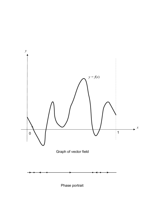
Figure 1: Example of a vector field of a structurally stable dynamical system on the circle $\mathbb{S}$, represented as the unit interval, and its phase portrait.

That is, $f$ is a periodic function of period one. This can be simplified by restricting to one period, namely the unit interval $0\leq x\leq 1$ such that $f(0)=f(1)$. Then (2) becomes

$$\dot{x}=f(x)\text{,}\qquad f(1)=f(0).$$ (3)

In this context the function $f$ is called a vector field. The vector field on $\mathbb{S}^{1}$ of class $C^{k}$ is a function that has $k$ continuous derivatives where each derivative is identified at the end points; i.e. $f:[0,1]\rightarrow\mathbb{R}$ such that $f^{(m)}(0)=f^{(m)}(1)$ $\forall\,0\leq m\leq k$. An example of this would be the graph in Fig 1.

2 Some Key Definitions

Before we begin discussing our main results, let us introduce some definitions that are to play key roles in our work. We shall assume in the sequel that all of our dynamical systems are at least $C^{1}$.

Definition 1.

A fixed point $x_{\ast}$ of (3) is one such that $f(x_{\ast})=0$, and is said to be hyperbolic if $f^{\prime}(x_{\ast})\neq 0$, otherwise it is said to be nonhyperbolic.

Definition 2.

A map $h:M\rightarrow M$, where $M$ is a manifold, is said to be a homeomorphism if it is a bijective bicontinuous map.

For example in [3] it is shown the maps $h:(0,\infty)\rightarrow(0,1)$ defined by $h=1/(1+x^{2})$ and $h:\mathbb{S}^{1}\rightarrow\mathbb{S}^{1}$ defined by $h(x)=x+a\cos x$ for $|a|<1$ are homeomorphisms.

Definition 3.

Two dynamical systems $\dot{x}=f(x)$ and $\dot{y}=g(y)$ on $M$ are topologically equivalent if there is a homeomorphism $h$ of $M$ such that $h$ maps oriented (by incresing time) orbits of the first system onto oriented orbits of the second system. Such an $h$ is called a topological equivalence between the systems (or sometimes a conjugacy - especially for the case of discrete dynamical systems).

It is easy to verify that a rotation of $-\pi/2$ radians, which corresponds to $y=h(x)=x-1/4$ for the $\operatorname{mod}1$ representation, is a topological equivalence between the dynamical systems $\dot{\theta}=\sin\theta$ and $\dot{\phi}=\cos\phi$ on the circle $\mathbb{S}^{1}$. A two-dimensional example (in the plane $\mathbb{R}^{2}$) in [6] shows that the linear system $\dot{x}=Ax$ is topologically equivalent to $\dot{y}=By$ where

$$A=\left[\begin{array}[c]{cc}-1&-3\\ -3&-1\end{array}\right]\quad\text{and}\quad B=\left[\begin{array}[c]{cc}2&0\\ 0&-4\end{array}\right]$$

via the homeomorphism

$$h(x)=\frac{1}{\sqrt{2}}\left[\begin{array}[c]{cc}1&-1\\ 1&1\end{array}\right]x.$$

To see this we note that the origin is the only fixed point of both systems, and for any other $(x_{1}^{0},x_{2}^{0})$, $h$ maps the solution of $\dot{x}=Ax$ beginning at this initial point onto the solution $(y_{1}^{0}e^{2t},y_{2}^{0}e^{-4t})$, with $(y_{1}^{0},y_{2}^{0})=h\left((x_{1}^{0},x_{2}^{0})\right)=1/\sqrt{2}\left(x_{1}^{0}-x_{2}^{0},x_{1}^{0}+x_{2}^{0}\right).$

Definition 4.

Denote the class of $C^{1}$ maps of the circle by $C^{1}(\mathbb{S}^{1})$. Then

$$\left\|f\right\|_{1}:=\sup\{\left|f(x)\right|:x\in\mathbb{S}^{1}\}+\sup\{\left|f^{\prime}(x)\right|:x\in\mathbb{S}^{1}\}$$

defines a norm on $C^{1}(\mathbb{S}^{1})$ called the $C^{1}$ norm. This norm generates a topology, called the $C^{1}$-topology, in the usual way via the open $\epsilon$-balls $B_{\epsilon}^{1}(f):=\{g\in C^{1}(\mathbb{S}^{1}):\left\|g-f\right\|_{1}<\epsilon\}$.

Definition 5.

The dynamical systems $\dot{x}=f(x)$ with $f\in C^{1}(\mathbb{S}^{1})$ is said to be $C^{1}$ structurally stable if for every $\epsilon>0$ sufficiently small, all $g\in B_{\epsilon}^{1}(f)$ are topologically equivalent to $f$.

We note that it is not difficult to imagine how these last two definitions can be generalized to any finite-dimensional closed (compact and without boundary) manifolds.

It is useful to take note of the following rather simple characterization of topological equivalence for a pair of $C^{1}$ dynamical systems, (i) $\dot{x}=f(x)$ and (ii) $\dot{y}=g(y)$ on the unit circle $\mathbb{S}^{1}$: A homeomorphism $h:S^{1}\rightarrow S^{1}$ is a topological equivalence from (i) to (ii) if and only if

$$h\left(\{x\in\mathbb{S}^{1}:f(x)=0\}\right) =\{y\in\mathbb{S}^{1}:g(y)=0\},\;h\left(\{x\in\mathbb{S}^{1}:f(x)>0\}\right)=\{y\in\mathbb{S}^{1}:g(y)>0\}\text{ and}$$

$$\text{ }h\left(\{x\in\mathbb{S}^{1}:f(x)<0\}\right) =\{y\in\mathbb{S}^{1}:g(y)<0\}.$$ (TE)

2.1 Bump functions

Throughout the necessity portion of the proof of the one-dimensional analog of Theorem P, we will be using bump functions. A simple example of a bump function is $\psi:\mathbb{R}\rightarrow\mathbb{R}$ defined as (4) and plotted in Fig 2.

$$\psi(x):=\begin{cases}e^{\frac{-1}{1-x^{2}}}&\text{for}\;x\in(-1,1),\\ 0&\text{for}\;x\notin(-1,1);\end{cases}$$ (4)

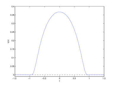
Figure 2: Example of a bump function.

Now, we can restrict the bump to any ball, which for our proof will correspond to an interval of our choice. Let $x_{0}$ be the center of the ball, and $r$ $(>0)$ be the radius. Then, denoting the ball as $B_{r}\left(x_{0}\right):=\{x\in\mathbb{R}:$ $\left|x-x_{0}\right|<r\}$, our bump function becomes

$$\psi(x):=\begin{cases}\exp\left(\frac{-r^{2}}{r^{2}-(x-x_{0})^{2}}\right)&\text{for}\;x\in B_{r}(x_{0}),\\ 0&\text{for}\;x\notin B_{r}(x_{0});\end{cases}$$ (5)

This can be specified to any interval $[a,b]$, which corresponds to a ball centered at $(a+b)/2$ with a radius of $(b-a)/2$: namely,

$$\psi(x):=\begin{cases}\exp\left(-\left(\frac{b-a}{2}\right)^{2}\middle/\left[\left(\frac{b-a}{2}\right)^{2}-\left(x-\frac{a+b}{2}\right)^{2}\right]\right)&\text{for}\;x\in(a,b),\\ 0&\text{for}\;x\notin(a,b);\end{cases}$$ (6)

We also note that that it can be easily verified using basic calculus that the bump function (6) satisfies

$$\left\|\psi\right\|_{1}<e^{-1}\left[1+6e^{-1}(b-a)^{-1}\right],$$ (7)

so once the interval has been specified, for every $\epsilon>0$ there exists a $\sigma>0$ such that $\left\|\sigma\psi\right\|_{1}<\epsilon$. This will be an important fact to keep in mind for the necessity portion of our proof. In many instances we will use a scaled bump function to obtain small $C^{1}$ perturbations of given functions in $C^{1}(\mathbb{S}^{1})$.

3 Peixoto’s Theorem on $\mathbb{S}^{1}$

We note that every closed one-dimensional manifold is homeomorphic to a circle, as shown in [4]. So, it suffices to restrict our attention to $\mathbb{S}^{1}$ in the one-dimensional analog of Theorem P that follows.

Theorem 1.

Suppose (3) is a $C^{1}$ dynamical system on $\mathbb{S}^{1}$. Then (3) is $C^{1}$ structurally stable if and only if it has finitely many fixed points, all of which are hyperbolic.

Proof.

For sufficiency, let us first prove the result for a dynamical system with no fixed points. Suppose (3) has no fixed points, then $|f(x)|>0$ on $[0,1]$. With out loss of generality, assume $f$ is positive, which means the phase space consists of a single periodic counterclockwise orbit. Since $f$ is continuous, there is an $\epsilon_{0}>0$ such that $f(x)>\epsilon_{0}\;\forall\,x\in[0,1]$. Consider the dynamical system

$$\dot{y}=g(y),$$ (8)

where $g\in C^{1}(\mathbb{S}^{1})$. If

$$\left\|g-f\right\|_{1}<\epsilon<\epsilon_{0},$$ (9)

then $g$ must also be positive on $\mathbb{S}^{1}$. Therefore, it follows from (TE) that the identity map is a topological equivalence, so (3) is structurally stable.

Next we prove the result for finitely many hyperbolic fixed points. Suppose $f(x_{k})=0$ and $f^{\prime}(x_{k})\neq 0$ for $k=1,2,\ldots,m$. We may assume none of them is an endpoint of the unit interval, since this can always be accomplished via a simple translation of the period interval. Let us order them as follows:

$$x_{k}<x_{k+1},k=1,2,\ldots,m-1\quad\text{and}\quad x_{m}<x_{1}.$$

We use this ordering to make it more understandable when speaking about “sequential” points. Notice, the end points are between the fixed points $x_{m}$ and $x_{1}$ and the non-fixed orbits are just open intervals between sequential points.

We observe that between any two sequential fixed points, $f$ does not change sign, and in some $\delta$-neighborhood of every fixed point, $f^{\prime}$ is nonzero owing to the hyperbolicity and continuity. So, we can select $\epsilon_{0}$ and $\delta>0$ small enough such that $|f^{\prime}(x)|\geq 2\epsilon_{0}$ on $[x_{k}-\delta,x_{k}+\delta]$ for $k=1,2,\ldots,m$, where the intervals $[x_{k}-\delta,x_{k}+\delta]$ are disjoint. Hence, $f$ is monotonic and has a single zero on each of these intervals. Now define $K(\delta)$ as the closure of the complement of these intervals, which is just a disjoint union of closed intervals itself. Since $f$ does not change sign between any two sequential fixed points, $f$ is nonvanishing in $K(\delta)$. Furthermore, it follows from continuity of $f$ that there is $0<\epsilon_{1}<\epsilon$ such that $|f(x)|\geq 2\epsilon_{1}\;\forall\,x\in K(\delta)$.

Now we show that structural stability is satisfied; in particular, for any $g\in C^{1}(\mathbb{S}^{1})$ satisfying

$$\left\|f-g\right\|_{1}<\epsilon<\min\{\epsilon_{0},\epsilon_{1}\}$$ (10)

the dynamical system (8) is topologically equivalent to (3). That is, there is a homeomorphism $h:\mathbb{S}^{1}\rightarrow\mathbb{S}^{1}$ mapping oriented orbits of (8) to (3). By (10), $g$ has exactly one zero, denoted as $y_{k}$, on each interval $[x_{k}-\delta,x_{k}+\delta]$ and no zeros on $K(\delta)$, and furthermore $g^{\prime}(y_{k})\neq 0$ and $g$ has the same sign on $(y_{k},y_{k+1})$ as $f$ does on $(x_{k},x_{k+1})$ whenever $1\leq k\leq m$. We select $h$ to be a piecewise linear homeomorphism with the following properties: $h(0)=h(1)=0$ and also $h(x_{k})=y_{k}$ for $k=1,2,\ldots,m$, and linear on the intervals $(0,x_{1}),(x_{1},x_{2}),\ldots,(x_{m-1},x_{m}),(x_{m},1)$; namely

$$h(x):=\left\{\begin{array}[c]{cc}\left(\frac{y_{1}}{x_{1}}\right)x,&0\leq x\leq x_{1}\\ \frac{\left(y_{k+1}-y_{k}\right)x+\left(y_{k}x_{k+1}-x_{k}y_{k+1}\right)}{\left(x_{k+1}-x_{k}\right)},&x_{k}\leq x\leq x_{k+1},1\leq k\leq m-1\\ \left(\frac{y_{m}}{x_{m}-1}\right)(x-1),&x_{m}\leq x\leq 1\end{array}\right.$$

This proves the sufficiency of the hypothesis owing to (TE).

For necessity, we show that if the fixed point hypothesis is not satisfied, then (3) is not structurally stable. In order to show this, we need to analyze all the cases in which the hypothesis may be violated. In each case we show if we add an arbitrarily small $C^{1}$ perturbation, $\eta$, of the right form to the original system, $g(x)=f(x)+\eta(x)$, we obtain a system that is not topologically to (3). The analysis is to be done in neighborhoods of nonhyperbolic fixed points, with the intention of showing that an arbitrarily small perturbation can change the homeomorphism type of the original fixed point set, thus insuring in view of (TE) that the perturbed system cannot be topologically equivalent to the original.

Case 1: An isolated nonhyperbolic fixed point $x_{\ast}$ across which $f$ does not change sign. It can be assumed, without loss of generality, that $f(x)>0$ in some punctured neighborhood $\mathring{B}_{\delta}(x_{\ast}):=B_{\delta}(x_{\ast})\smallsetminus\{x_{\ast}\}$ of $x_{\ast}$ as shown in Fig 3.

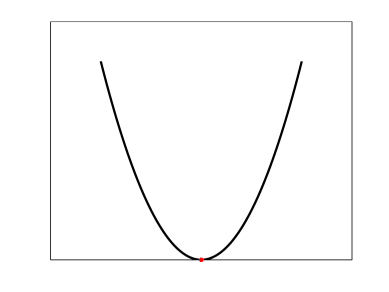
Figure 3: An example of a function in a neighborhood of a nonhyperbolic fixed point with the aforementioned properties.

Note that if $x_{\ast}$ is the only fixed point, the perturbation $g(x)=f(x)+\epsilon$ defines a dynamical system with an empty fixed point set, denoted as $g^{-1}(0)=\varnothing$, while $f^{-1}(0)=\{x_{\ast}\}$, so it follows from (TE) that $\dot{x}=f$ and $\dot{y}=g$ are topologically inequivalent.

If $x_{\ast}$ is not unique, we have to localize the above analysis. In order to do this we would like to perturb the system in such a way as to annihilate the fixed point without affecting anything outside of the neighborhood. This can be accomplished by using a bump function (cf. section 2.1).

Since $x_{\ast}$ is the only fixed point, which we may assume is not an end point of the unit interval, in $(x_{\ast}-\delta,x_{\ast}+\delta)$, we define

$$\psi(x):=\begin{cases}\exp\left(\frac{-\delta^{2}}{\delta^{2}-(x-x_{\ast})^{2}}\right)&\text{for}\;x\in(x_{\ast}-\delta,x_{\ast}+\delta),\\ 0&\text{for}\;x\notin(x_{\ast}-\delta,x_{\ast}+\delta);\end{cases}$$ (11)

It follows from (7) that for any $\epsilon>0$, there exists a $\sigma>0$ such that $\left\|\sigma\psi\right\|_{1}<\epsilon$. Hence, if $g=f+\sigma\psi$, $\left\|f-g\right\|_{1}<\epsilon$ and $\dot{y}=g$ has no fixed point in $(x_{\ast}-\delta,x_{\ast}+\delta)$. Consequently, $f^{-1}(0)$ and $g^{-1}(0)$ cannot be homeomorphic, which means that $f$ is not structurally stable.

Case 2: An isolated nonhyperbolic fixed point $x_{\ast}$ across which $f$ changes sign, which can be assumed, without loss of generality, to be as shown in Fig. 4. Again, we define $\delta>0$ such that $f$ is not zero in $\mathring{B}_{\delta}(x_{\ast})$ .

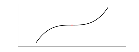
Figure 4: An example of a function in a neighborhood of a nonhyperbolic fixed point with the aforementioned properties.

For this case, we shall show there is an arbitrarily small $C^{1}$ perturbation confined to $B_{\delta}(x_{\ast})$, which has three hyperbolic fixed points in this interval instead of one nonhyperbolic one.

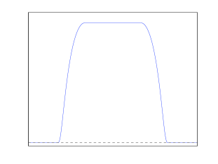
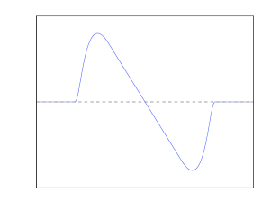
Figure 5: Example plots of equations 12 and 13 respectively.

First, we put two bump functions together to create a new bump function that is equal to $e^{-1}$ in the closed interval $[x_{\ast}-\delta/2,x_{\ast}+\delta/2]$ and vanishes in the complement of $(x_{\ast}-\delta,x_{\ast}+\delta)$; namely,

$$\varphi(x):=\left\{\begin{array}[c]{cc}\exp\left(-\left(\frac{\delta}{2}\right)^{2}\middle/\left[\left(\frac{\delta}{2}\right)^{2}-\left(x-x_{\ast}+\frac{\delta}{2}\right)^{2}\right]\right),&x_{\ast}-\delta<x\leq x_{\ast}-\delta/2\\ e^{-1},&x_{\ast}-\delta/2\leq x\leq x_{\ast}+\delta/2\\ \exp\left(-\left(\frac{\delta}{2}\right)^{2}\middle/\left[\left(\frac{\delta}{2}\right)^{2}-\left(x_{\ast}-x+\frac{\delta}{2}\right)^{2}\right]\right),&x_{\ast}+\delta/2\leq x<x_{\ast}+\delta\\ 0,&x\notin(x_{\ast}-\delta,x_{\ast}+\delta)\end{array}\right\}.$$ (12)

Observe that this function is $C^{\infty}$ on the whole real line except at the points $x_{\ast}-\delta/2$ and $x_{\ast}+\delta/2$ where it is only $C^{1}$. Next, we define

$$\vartheta(x):=-\frac{2(x-x_{\ast})\varphi(x)}{\delta e}$$ (13)

Examples of (12) and (13) are given in Fig 5.

Note, as usual, for each $\epsilon>0$ there exists a $\sigma>0$ such that $\left\|\sigma\vartheta\right\|_{1}<\epsilon$. Moreover, $g:=f+\sigma\vartheta$ has a zero at $x_{\ast}$ with $g^{\prime}(x_{\ast})<0$ and just two other zeros in $B_{\delta}(x_{\ast})$ at points $x_{\ast}\pm\nu$, with $0<\nu<\delta$, and $g^{\prime}(x_{\ast}-\nu)=g^{\prime}(x_{\ast}+\nu)>0$. As $\left\|f-g\right\|_{1}<\epsilon$ and $f^{-1}(0)$ and $g^{-1}(0)$ are not homeomorphic, (TE) implies that $f$ is not structurally stable.

Case 3: An interval of (nonhyperbolic) fixed points, i.e. $f(x)=0$ on some interval $[a,b]\subseteq[0,1]$. If $[a,b]=[0,1]$, the addition of an arbitrarily small positive constant changes the fixed point set from all of $\mathbb{S}^{1}$ to the empty set, which proves that such a system cannot be $C^{1}$structurally stable. On the other hand, if the interval is a proper subset of the unit interval, we may assume that $[a,b]\subseteq\left(0,1\right)$ and it is isolated from any other points in the fixed point set of $\dot{x}=f$. Accordingly, there is a positive $\delta$ such that $[a-\delta,b+\delta]\subset\left(0,1\right)$ and $[a-\delta,b+\delta]\cap f^{-1}\left(0\right)=[a,b]$. By analogy with Case 1 and Case 2 above, we consider two subcases: (i) $f$ has the same sign in $(a-\delta,a)$ and $(b,b+\delta)$; and (ii) $f$ has opposite signs in $(a-\delta,a)$ and $(b,b+\delta)$. Naturally, we may assume without loss of generality the the sign in (i) is positive, and in (ii) it goes from negative to positive. It is convenient to use the following analog of the bump function $\varphi$ for both (i) and (ii):

$$\hat{\varphi}(x):=\left\{\begin{array}[c]{cc}\exp\left(-\left(\frac{\delta}{2}\right)^{2}\middle/\left[\left(\frac{\delta}{2}\right)^{2}-\left(x-a+\frac{\delta}{2}\right)^{2}\right]\right),&a-\delta<x\leq a-\delta/2\\ e^{-1},&a-\delta/2\leq x\leq b+\delta/2\\ \exp\left(-\left(\frac{\delta}{2}\right)^{2}\middle/\left[\left(\frac{\delta}{2}\right)^{2}-\left(b-x+\frac{\delta}{2}\right)^{2}\right]\right),&b+\delta/2\leq x<b+\delta\\ 0,&x\notin(a-\delta,b+\delta)\end{array}\right..$$ (14)

Inasmuch as for any $\epsilon>0$ there is a $\sigma>0$ such that $\left\|\sigma\phi\right\|_{1}<\epsilon$, in subcase (i) the perturbation $\dot{y}=g=f+\sigma\phi$ satisfies has $\left\|f-g\right\|_{1}<\epsilon$ and has no fixed points in $[a-\delta,b+\delta]$, which means it cannot be topologically equivalent to $\dot{x}=f$ in virtue of (TE). While for subcase (ii), the perturbation $\dot{y}=g$, where

$$g:=f+\sigma\hat{\vartheta},$$

with

$$\hat{\vartheta}(x):=-\frac{2\hat{\varphi}(x)}{e\left(a+b\right)}\left(x-\frac{a+b}{2}\right),$$ (15)

produces an arbitrarily small $C^{1}$ perturbation of $\dot{x}=f$ having precisely three hyperbolic fixed points in $[a-\delta,b+\delta]$. Therefore, $f$ is not structurally stable for any of these subcases.

Although there remain some situations for which the hypothesis of the theorem does not hold, we have actually introduced the bump function methodology which can be readily seen to be capable of disposing of the remaining cases. Consequently, we leave the remaining details of the proof to the reader, with the following very interesting exception.

Case 4: Suppose $\dot{x}=f$ has distinct fixed points $x_{1},x_{2},x_{3},\ldots$ and $x_{n}\rightarrow x_{\ast}$ , so that $x_{\ast}$ is a fixed point and the limit of the sequence $\{x_{n}\}$, which may be assumed to lie in an open interval $J=(x_{\ast}-r,x_{\ast}+r)$ contained in $(0,1)$, which contains no other fixed points. The sequence might consist of all hyperbolic fixed points as shown in Fig 6, or it might be comprised of some combination of hyperbolic fixed points and and nonhyperbolic fixed points of the types treated in Cases 1 and 2.

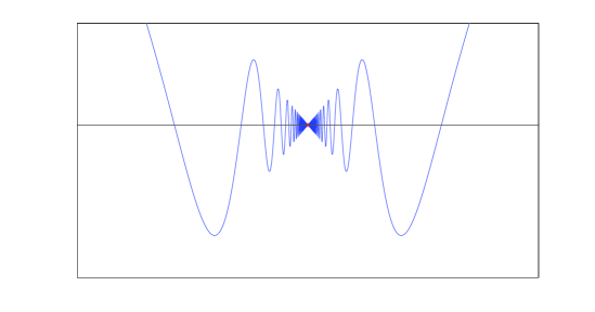
Figure 6: An example of a function with fixed points having the aforementioned properties.

Notice that $\{x_{n}\}$ is countably infinite, so that if we perturb the system $\dot{x}=f$ to a system $\dot{y}=g$ with only finitely many fixed points in $J$, and the same fixed points in the complement of $J$, the two systems must be topologically inequivalent.

Since $f$ is $C^{1}$, for any $\epsilon>0$ there is a positive $\delta=\delta(\epsilon)<\epsilon$ such that $|x-x_{\ast}|<\delta$ implies $\left|f(x)\right|=|f(x)-f(x_{\ast})|<\epsilon\left|x-x_{\ast}\right|$. Furthermore, there are only finitely many fixed points in $J\smallsetminus B_{s}(x_{\ast})$ for any $0<s<r$. Let us use the bump function

$$\psi(x):=\begin{cases}\exp\left(\frac{-\delta^{2}}{\delta^{2}-(x-x_{\ast})^{2}}\right)&\text{for}\;x\in(x_{\ast}-r/2,x_{\ast}+r/2),\\ 0&\text{for}\;x\notin(x_{\ast}-r/2,x_{\ast}+r/2);\end{cases},$$ (16)

and for any given $\epsilon>0$ choose $\sigma>0$ such that $\left\|g-f\right\|_{1}=\left\|\left(f+\sigma\upsilon\right)-f\right\|_{1}<\epsilon$. Then $g$ has no zeros in $B_{s}(x_{\ast})$ for some $0<s<r/2$ and so only finitely many fixed points in $J$, which means that $f$ is not structurally stable. This completes our proof.

∎

4 Density Theorem on $\mathbb{S}^{1}$

We now prove the one-dimensional analog of the density part of Theorem P. It is convenient to introduce the following notation towards this end. Define $SS^{1}\left(\mathbb{S}^{1}\right)$ to be the $C^{1}$-structurally stable systems $\dot{x}=f$ on $C^{1}\left(\mathbb{S}^{1}\right).$

Theorem 2.

The set of dynamical systems $SS^{1}\left(\mathbb{S}^{1}\right)$ is $C^{1}$ open and dense in $C^{1}\left(\mathbb{S}^{1}\right).$

Proof.

The openness follows directly from the sufficiency proof of Theorem 1, and the density is essentially a straightway consequence of the necessity argument for the same theorem. In particular, it was shown in the sufficiency proof that the fixed point hypothesis is preserved under sufficiently small perturbations, and so $SS^{1}\left(\mathbb{S}^{1}\right)$ is a $C^{1}$ open subset of $C^{1}\left(\mathbb{S}^{1}\right)$.

It is clear from the methods used in proving the necessity part of Theorem 1, that for any $C^{1}$ dynamical system $\dot{x}=f$ on $\mathbb{S}^{1}$ there is an arbitrarily small $C^{1}$ perturbation $\dot{y}=g$ such that $g$ has only finitely many zeros. Then, using the bump function methods employed for Cases 1 and 2 of the necessity in Theorem 1, we can obtain a further arbitrarily small perturbation $\dot{z}=h$ with only hyperbolic fixed points. This completes the proof.

∎

It is worth noting that one could have used several other types of bump function based perturbations in the above proofs of the necessity of the hyperbolic hypothesis in Theorem 1 and the density result in Theorem 2. For example, the functions $\vartheta$ and $\hat{\vartheta}$ used for Case2 and Case 3 (ii), respectively, in the necessity proof of Theorem 1 could be replaced with an appropriate form of the derivative of a bump function, as is evident from the plot of the first and second derivatives of the simple bump function (4) given in Fig 7.

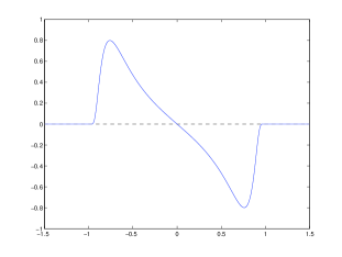
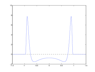
Figure 7: The first and second derivatives, respectively, of the simple bump function.

Finally, it is interesting to remark that the proofs of both Theorems 1 and 2 can be reduced to just a few lines by the application of a standard transversality theorem described for example in [2], which is an indication of the importance of differential topology in the modern theory of dynamical systems.

5 Conclusion

The epochal structural stability and density theorems of Peixoto for dynamical systems on closed surfaces have long and complicated proofs involving concepts unfamiliar to many undergraduate enthusiasts. In this note we have demonstrated that the one-dimensional analogs of these theorems can be proved using methods that are well known to most undergraduate mathematics majors, thus providing a useful introduction to many of the elements of the two-dimensional proofs. One might well imagine that Peixoto himself considered the one-dimensional version and used it, along with the pioneering efforts of Andronov and Pontryagin, as a guide for his theorems.

6 Acknowledgement

I would like to thank Professor Denis Blackmore of the Department of Mathematical Sciences at New Jersey Institute of Technology for suggesting this project - which he often sketched when teaching dynamical systems courses - and for his constant encouragement and advice in bringing it to fruition. In addition, I would like to thank my friends Tom, Heather, and Ivana for giving me early feedback on the readability of this note.

References

- [1] A. Andronov and L. Pontryagin. Systèmes grossiers. Dokl. Akad. Nauk. SSSR, 14:247–251, 1937.
- [2] V. Guillemin and A. Pollack. Differential Topology. Prentice-Hall, 1974.
- [3] J. Meiss. Differential Dynamical Systems. SIAM, Philadelphia, PA, 2007.
- [4] J. Milnor. Topology from the Differentiable Viewpoint. Princeton University Press, 1997.
- [5] M. Peixoto. Structural stability on two-dimensional manifolds. Topology, 1:101–120, 1962.
- [6] L. Perko. Differential Equations and Dynamical Systems. Springer-Verlag, New York, NY, 3 edition, 2001.
- [7] S. Strogatz. Nonlinear Dynamics and Chaos. Westview Press, Cambridge, MA, 1994.