ABSTRACT: A simple discrete planar dynamical model for the ideal (logical) R-S flip-flop circuit is developed with an eye toward mimicking the dynamical behavior observed for actual physical realizations of this circuit. It is shown that the model exhibits most of the qualitative features ascribed to the R-S flip-flop circuit, such as an intrinsic instability associated with unit set and reset inputs, manifested in a chaotic sequence of output states that tend to oscillate among all possible output states, and the existence of periodic orbits of arbitrarily high period that depend on the various intrinsic system parameters. The investigation involves a combination of analytical methods from the modern theory of discrete dynamical systems, and numerical simulations that illustrate the dazzling array of dynamics that can be generated by the model. Validation of the discrete model is accomplished by comparison with certain Poincaré map like representations of the dynamics corresponding to three-dimensional differential equation models of electrical circuits that produce R-S flip-flop behavior.

Keywords: R-S flip-flop, discrete dynamical system, Poincaré map, bifurcation, chaos, transverse homoclinic orbits

AMS Subject Classification: 37C05, 37C29, 37D45, 94C05

1 Introduction

The ideal R-S flip-flop circuit is a logical feedback circuit that can be described most efficiently in terms of Fig. 1, with input/output behavior described in Table 1, which shows the set ($S$) and reset ($R$) inputs feeding into the simple circuit comprised of two nor gates and the corresponding outputs $Q$ and $P$ that are generated. The input to this circuit may be represented as $(S,R)$ and the output by $(Q,P)$, so the association of the input to the output, denoted by $(S,R)\rightarrow(Q,P)$ may be regarded as the action of a map from the plane $\mathbb{R}^{2}:=\{(x,y):x,y\in\mathbb{R}\}$ into itself, where $\mathbb{R}$ denotes the real numbers. Our goal, from this mapping perspective, is to construct a simple nonlinear map of the plane that models the logical properties of the R-S flip-flop circuit, with iterates (discrete dynamics) that at least qualitatively capture most of its interesting dynamics, both those that are intuitive and those that have been observed in studies of physical circuit simulations - especially in certain critical cases that we shall describe in the sequel.

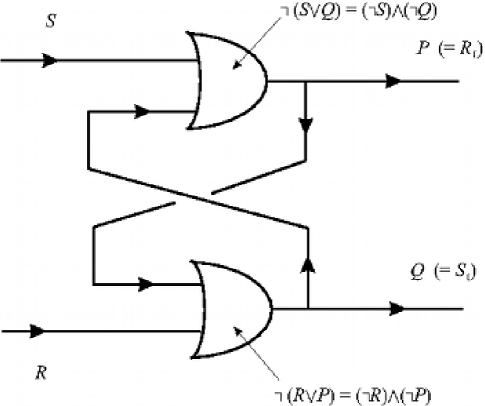
Figure 1: $R$-$S$ flip-flop circuit

The binary input/output behavior, with 0 and 1 representing false and true, respectively, is given in the following table.

$S$	$R$	$S_{1}:=Q$	$R_{1}:=P$
1	0	$\begin{array}[c]{c}1\end{array}$	$\begin{array}[c]{c}0\end{array}$
0	1	$\begin{array}[c]{c}0\end{array}$	$\begin{array}[c]{c}1\end{array}$
1	1	$\begin{array}[c]{c}0\end{array}$	$\begin{array}[c]{c}0\end{array}$
0	0	or $\ \begin{array}[c]{c}1\\ 0\end{array}$	or $\begin{array}[c]{c}0\\ 1\end{array}$

Table 1. Binary input/output of $R$-$S$ flip-flop circuit

Note that the input/output behavior is not well defined when the set and reset values are both $0$; a situation that can be remedied by identifying $(1,0)$ with $(0,1)$. Such an identification strategy is consistent with the obvious symmetry of the circuit with respect to $S$ and $R$, and in fact we shall employ this in the sequel when we describe and analyze our $R$-$S$ flip-flop map model. If we make this symmetry identification, it leads to an unambiguous input/output behavior for the circuit, and from an abstract perspective, it is not immediately clear why the state $(1,1)$ should be problematical - other than that it is the only state that produces non-complementary output values $0,0$. Notwithstanding the well defined behavior of the abstract R-S flip-flop circuit when the symmetry identification is imposed, actual physical circuit models comprised of elements such as capacitors, diodes, inductors and resistors exhibit highly oscillatory, very unstable and even chaotic dynamics (metastable operation), as experimentally observed in such studies as [4, 14, 15, 17]. This type of highly irregular dynamical behavior has also been found in R-S flip-flop realizations in the context of Josephson junctions [27]. In general, it is found that physical models of R-S flip-flop circuits invariably generate very complex dynamics belying the simplicity of the abstract logical circuit, which can plausibly be ascribed to the fact that every real model of this circuit must have inherent time sequencing characteristics due to the finite speed of electromagnetic waves.

Continuous dynamical systems representations of R-S flip-flop circuits derived from the usual circuit equations applied to the physical models, typically lead to three-dimensional systems of first order, autonomous, (possibly discontinuous) piecewise smooth (and usually piecewise linear) differential equations such as those investigated by Murali et al. [20], Okazaki et al. [21] and Ruzbehani et al. [23]. These mathematical models are traceable back to the pioneering work of Moser [19], and are subsumed by the famous circuit of Chua and its generalizations [5, 6]. Experimental observations on real circuit models of R-S flip-flops, together with numerical simulations utilizing such tools as SPICE [11], and analytical studies employing the tools of modern dynamical systems theory (see e.g. [9, 16, 22, 26]) including Poincaré sections and Melnikov functions such as in [6, 8, 15, 21, 23] have painted a rather compelling picture of the extreme complexity of the dynamical possibilities.

Naturally, when one has a series of quite successful mathematical representations of phenomena or processes as is the case for R-S flip-flop circuit behavior, it leads to the question of the possible existence of simpler models. One cannot expect to reduce the dimension of the continuous dynamical models, since it is impossible for two-dimensional systems of autonomous differential equations to have chaotic solutions. However, two-dimensional discrete dynamical systems are an enticing possibility since they can exhibit almost all types of complex dynamics - including chaotic regimes. Moreover, there have been some studies, albeit just a few, including those of Danca [8] and Hamill et al. [10], which give strong indications of the potential of modeling circuits such as the R-S flip-flop using two-dimensional difference equations or iterated planar maps. Encouraged by this literature on discrete dynamical models and relying heavily on our knowledge of dynamical systems theory and physical intuition, we have developed a discrete - essentially phenomenological -dynamical model generated by iterates of a rather simple nonlinear (quadratic), two-parameter planar map, which we present and analyze in this paper.

Our investigation is organized as follows. First, in Section 2, we define our simple planar map model - with iterates producing the dynamic behavior that we shall show mimics that observed in real R-S flip-flop circuits. Moreover, we derive some basic properties of the map related to fixed points and the existence of a local inverse. This is followed in Section 3 with a more thorough analysis of the fixed points of the map - including a local stability analysis and an analysis of stable and unstable manifolds - under very mild, and quite reasonable, restrictions on the two map parameters. Next, in Section 4, we fix the value of one of the parameters and prove the existence of a Hopf bifurcation at an interior fixed point as the other parameter is varied. We also note what appears to be a kind of Hopf bifurcation cascade (manifested by an infinite sequence) as the parameter is increased, which suggests the existence of extreme oscillatory behavior culminating in chaos. We then prove the existence of chaotic dynamics in Section 5. This is followed in Section 6 by a comparison of the dynamics of our model with other results in the literature, primarily from the perspective of planar Poincaré maps. Naturally, liberal use is made in this section of numerical simulations of our model for comparison purposes. Finally, in Section 7, we summarize and underscore some of the more important results of this investigation, and identify several interesting directions for future related research.

2 A Discrete Model

Based upon the ideal mathematical properties of the R-S flip-flop circuit, which were briefly delineated in the preceding section, and a knowledge of the interesting dynamical characteristics of actual physical circuits constructed to perform like the R-S flip-flop circuit (see e.g. [10, 15, 21, 23, 27], and also [8] for related results) , we postulate the following simple, quadratic, two-parameter planar map model:

$$\Phi=\left(\varphi,\psi\right)=\Phi_{\lambda,\mu}=\left(\varphi_{\lambda,\mu},\psi_{\lambda,\mu}\right):\mathbb{R}^{2}\rightarrow\mathbb{R}^{2},$$ (1)

where $\lambda$ and $\mu$ are positive parameters, and the coordinate functions $\varphi$ and $\psi$ are defined as

$$\varphi\left(x,y\right) =\varphi_{\lambda,\mu}\left(x,y\right):=1-x\left[\lambda\left(1-x\right)+y\right],$$

$$\psi\left(x,y\right) =\psi_{\lambda,\mu}\left(x,y\right):=\mu y\left(x-y\right)$$ (2)

Naturally, this map generates a discrete dynamical system - actually a discrete semidynamical system - in terms of its forward iterates determined by $n$-fold compositions of the map with itself, denoted as $\Phi_{\lambda,\mu}^{n}$, or more simply as $\Phi^{n}$, where $n$ is a nonnegative integer. We shall employ the usual notation and definitions for this discrete system; for example, the positive semiorbit of a point $p\in\mathbb{R}^{2}$, which we denote as $O_{+}(p)$, is simply defined as

$$O_{+}(p):=\left\{\Phi^{n}(p):n\in\mathbb{Z},\,n\geq 0\right\},$$

and all other relevant definitions are standard (cf. [9, 12, 16, 22, 26]). Our model map is clearly real-analytic, which we denote as usual by $\Phi\in C^{\omega}$ and a fortiori smooth, denoted as $\Phi\in C^{\infty}$.

Assuming the reset and set values, corresponding to the $x$- and $y$-coordinates, respectively, are normalized so that they may assume the discrete (logical) values $0$ or $1$, it makes sense to restrict the model map to the square $I^{2}:=I\times I:=[0,1]\times[0,1]$ in the plane. In fact, owing to the obvious symmetry of the circuit with respect to the reset and set inputs, it is actually natural to further restrict our attention to the triangular domain

$$T:=\left\{(x,y)\in\mathbb{R}^{2}:0\leq x\leq 1,\,0\leq y\leq x\right\},$$ (3)

but we shall defer additional discussion of this point until later, except to note here that

$$\Phi(0,0)=(1,0),\;\Phi(1,0)=(1,0)\text{ and }\Phi(1,1)=(0,0),$$ (4)

which shows that our model is at least logically consistent with the R-S flip-flop circuit.

2.1 Basic properties of the model

Before embarking on a more thorough dynamical analysis of the iterates of our simple map model, we shall describe some of its simpler properties. The fixed points of the map, satisfying $\Phi(x,y)=(x,y)$, are the solutions of the equations

$$1-x\left[\lambda\left(1-x\right)+y\right] =x$$

$$\mu y\left(x-y\right) =y,$$ (5)

from which we readily deduce the property.

• The points $(1,0)$ and $(1/\lambda,0)$ are fixed points of $\Phi$ for all $\lambda,\mu>0$ (cf. (4)), while all other fixed points are in the complement of the $x$-axis and are determined by the equations

  $$\left(1-\lambda\right)x^{2}+\left(1+\lambda-\mu^{-1}\right)x-1=0,\;y=x-\mu^{-1}.$$

  Hence, we have the following: there are no additional fixed points if $\lambda=1$ and $\mu^{-1}=1+\lambda=2$; there is one more fixed point, $(x,y)$ with

  $$x=\frac{\mu}{\mu(1+\lambda)-1},\;y=\frac{\mu}{\mu(1+\lambda)-1}-\frac{1}{\mu};$$

  if $\lambda=1$ and $\mu^{-1}\neq 1+\lambda=2$; and if $\lambda\neq 1$ and $\left(1+\lambda-\mu^{-1}\right)^{2}+4\left(1-\lambda\right)\geq 0$, there two additional fixed points $(x,y)$ with

  $$x=\frac{\left(\mu^{-1}-\lambda-1\right)\pm\sqrt{\left(1+\lambda-\mu^{-1}\right)^{2}+4\left(1-\lambda\right)}}{2\left(1-\lambda\right)},\;y=x-\frac{1}{\mu},$$ (6)

  while if $\left(1+\lambda-\mu^{-1}\right)^{2}+4\left(1-\lambda\right)<0$, there are only the two fixed points on the $x$-axis.

The following additional properties of the map follow directly from its definition.

• $\Phi$ maps the $x$-axis into itself, and if $0<\lambda\leq 4$, $\Phi$ actually maps the horizontal edge $e_{h}:=\{(x,0):0\leq x\leq 1\}$ of $T$ into itself.

• $\Phi$ maps the diagonal line $x-y=0$ into the $x$-axis, and maps the diagonal edge $e_{d}:=\{(x,x):0\leq x\leq 1\}$ of $T$ into $e_{h}$ if $0<\lambda\leq 2$.

• $\Phi$ maps the $y$-axis onto the portion of the line $x=1$ with $y\leq 0$, and maps the line $x=1$, containing the vertical edge $e_{v}:=\{(1,y):0\leq y\leq 1\}$ of $T$, onto the parabola $y=\mu x(1-x)$ passing through the origin and the fixed point $(1,0)$.

• It follows from the derivative (matrix)

  $$\Phi^{\prime}(x,y)=\left(\begin{array}[c]{cc}\lambda(2x-1)-y&-x\\ \mu y&\mu(x-2y)\end{array}\right)$$ (7)

  and the inverse function theorem that $\Phi$ is a local $C^{\omega}$-diffeomorphism at any point in the complement of the quadratic curve

  $$\lambda\left(2x-1\right)\left(x-2y\right)+2y^{2}=0,$$

  while in general, the preimage of any point in the plane, denoted as $\Phi^{-1}\left((x,y)\right)$, is comprised of at most four points.

3 Elementary Dynamics of the Model

We shall analyze the deeper dynamical aspects of the model map (1)-(2) for various parameter ranges in the sequel, but first we dispose of some of the more elementary properties such as a the usual local linear stability analysis of the fixed points. At this stage, and for the remainder of our investigation, we shall focus on the restriction of the model map to the triangle $T$ and assume that

($\mathcal{A}$1)$\qquad\qquad 0<\lambda<1<\mu$

With the above restriction and assumption, it follows from the preceding section that our model map has precisely four fixed points: two in $T$; one near $T$ at $(1/\lambda,0)$ when $\lambda$ is close to unity; and the final one rather distant from $T$. In the next subsection, we embark on a local stability analysis of the fixed points of $\Phi$ on or near the triangle $T$.

3.1 Local analysis of the fixed points

The local properties of the fixed points of our model map shall be delineated in a series of lemmas. They all have straightforward proofs that follow directly from the results in the preceding section and fundamental dynamical systems theory (as in [9, 16, 22, 26]), which are left to the reader.

Lemma 3.1. The fixed points of $\Phi$ on the $x$-axis, namely $(1,0)$ and $(1/\lambda,0)$, are a saddle and a source with eigenvalues (of $\Phi^{\prime}(1,0)$ and $\Phi^{\prime}(1/\lambda,0)$) $\lambda,\mu$ and $2-\lambda,\mu/\lambda$, respectively. For $(1,0)$, the stable manifold is

$$W^{s}\left(1,0\right)=\left\{(x,0):x<1/\lambda\right\},$$

and the linear unstable manifold is

$$W_{\ell}^{u}(1,0)=\left\{\left(x,(\lambda-\mu)(x-1)\right):x\in\mathbb{R}\right\}.$$

Lemma 3.2. The fixed point of $\Phi$ in the interior of $T$, which we denote as $p_{\ast}=(x_{\ast},y_{\ast})$, is defined according to (6) as

$$x_{\ast}=x_{\ast}(\lambda,\mu)=\frac{\left(\mu^{-1}-\lambda-1\right)+\sqrt{\left(1+\lambda-\mu^{-1}\right)^{2}+4\left(1-\lambda\right)}}{2\left(1-\lambda\right)},\;y_{\ast}=y_{\ast}(\lambda,\mu)=x_{\ast}-\frac{1}{\mu},$$

and has complex conjugate eigenvalues that are roots of the quadratic equation

$$\sigma^{2}-a\sigma+b=0,$$

where

$$a =a(\lambda,\mu):=\left(2\lambda-\mu-1\right)x_{\ast}+\left(2-\lambda+\mu^{-1}\right),\;$$

$$b =b(\lambda,\mu):=\mu\left\{\left[\lambda\left(4\mu^{-1}-1\right)-2(1+\mu^{-1})\right]x_{\ast}+2\left[1-\mu^{-1}\left(\lambda-\mu^{-1}\right)\right]\right\};$$

namely

$$\sigma =\sigma(\lambda,\mu)=\frac{1}{2}\left[a+i\sqrt{4b-a^{2}}\right]$$

$$\bar{\sigma} =\bar{\sigma}(\lambda,\mu)=\frac{1}{2}\left[a-i\sqrt{4b-a^{2}}\right].$$

Hence it is a spiral sink or spiral source, respectively, when

$$\left|\sigma\right|^{2}=\left|\bar{\sigma}\right|^{2}=b<1,$$

or

$$\left|\sigma\right|^{2}=\left|\bar{\sigma}\right|^{2}=b>1.$$

Otherwise (when $b=1$) it has neutral stability.

Lemma 3.3. For any fixed $\lambda$ and variable $\mu$ satisfying ($\mathcal{A}$1), the coefficient $b$ defined above satisfies the following properties:

• It is a smooth $(=C^{\infty})$, nonnegative function of $\mu$ for $\mu>1$, such that $db/d\mu>0$ for every $\mu>1$.

• $b\uparrow\infty$ as $\mu\uparrow\infty.$

• There exists a positive $c(\lambda)$ such that $b<1$ for $1<\mu<1+c(\lambda).$

• In particular, for each $0<\lambda<1$, there exists a unique $\mu_{h}=\mu_{h}(\lambda)=1+c(\lambda)$ such that $1<\mu_{h}$, $b(\lambda,\mu_{h})=1$, $0<b(\lambda,\mu)<1$ for $1<\mu<\mu_{h}$, and $b(\lambda,\mu)>1$ for $\mu_{h}<\mu$.

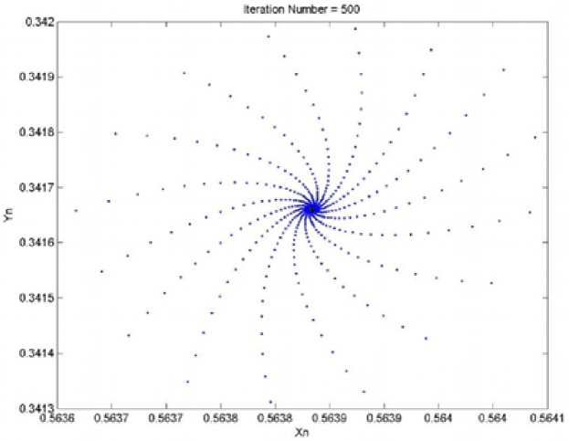
Figure 2: Spiral attractor at interior fixed point ($\cong(0.5639,0.3417)$) for $\lambda=0.99,\,\mu=4.5$. The initial point is $(x,y)=(0.564,0.342)$ and the eigenvalues are $\xi\cong-0.3763\pm 0.9171i$.

The case when the interior fixed point is a spiral attractor is shown in Fig. 2. By fixing $\lambda$ at a value near one, say $\lambda=0.99$, and then varying $\mu$ over a range from $4$ to $5$, we obtain a very rich array of dynamics as described in what follows.

4 Oscillation and Hopf Bifurcation

In order to achieve a reasonable amount of focus - given the wide range of possible model map parameters - we shall narrow our range of investigation by adhering to the following additional assumption in the sequel:

($\mathcal{A}$2)$\qquad\qquad\lambda=0.99=\frac{99}{100}.$

Then assuming ($\mathcal{A}$1) and ($\mathcal{A}$2), our map $\Phi=\Phi_{\mu}$ satisfies all the properties delineated above, and depends only on the single parameter $\mu\in(1,\infty)$. In particular, it follows directly from Lemma 3.2 that

$$x_{\ast}(\mu):=x_{\ast}(.99,\mu)=50\left\{\left(\mu^{-1}-1.99\right)+\sqrt{\left(1.99-\mu^{-1}\right)^{2}+0.04}\right\},\;y_{\ast}(\mu):=y_{\ast}(.99,\mu)=x_{\ast}-\frac{1}{\mu},$$ (8)

and

$$a(\mu) :=a(.99,\mu)=\left(.98-\mu\right)x_{\ast}+\left(1.01+\mu^{-1}\right),$$

$$b(\mu) :=b(.99,\mu)=\mu\left\{\left[(.99)\left(4\mu^{-1}-1\right)-2(1+\mu^{-1})\right]x_{\ast}+2\left[1-\mu^{-1}\left(.99-\mu^{-1}\right)\right]\right\}.\;$$ (9)

It is then straightforward to compute in the notation of Lemma 3.3 that

$$c:=c(.99)\cong 3.5438,\;\mu_{h}:\cong\mu_{h}(.99)\cong 4.5438,\;x_{\ast}(\mu_{h})\cong 0.5632,\;y_{\ast}(\mu_{h})\cong 0.3431.$$ (10)

In order to study the behavior of the map in a neighborhood of the fixed point $p_{\ast}=(x_{\ast},y_{\ast})$, it is convenient to translate the coordinates and map to the origin by defining

$$\hat{\Phi} :=\hat{\Phi}_{\mu}(\xi,\eta):=\Phi_{\mu}(\xi+x_{\ast},\eta+y_{\ast})-\Phi_{\mu}(x_{\ast},y_{\ast})$$

$$=\Phi_{\mu}(\xi+x_{\ast},\eta+y_{\ast})-(x_{\ast},y_{\ast}).$$ (11)

It is easy to compute that

$$\hat{\Phi}:=\hat{\Phi}_{\mu}(\xi,\eta)=\left(\hat{\varphi}_{\mu}(\xi,\eta),\hat{\psi}_{\mu}(\xi,\eta)\right),$$ (12)

where

$$\hat{\varphi}_{\mu}(\xi,\eta) :=\left[(0.98)x_{\ast}(\mu)+\mu^{-1}-0.99\right]\xi-x_{\ast}(\mu)\eta+\xi\left[(0.99)\xi-\eta\right],$$

$$\hat{\psi}_{\mu}(\xi,\eta) :=\left[\mu x_{\ast}(\mu)-1\right]\xi-\left[2-\mu x_{\ast}(\mu)\right]\eta+\mu\eta\left(\xi-\eta\right).$$ (13)

4.1 Invariant curve and Hopf bifurcation

Now with this simple quadratic representation of the model map with respect to the fixed point $p_{\ast}$ interior to the triangle $T$ is a straightforward matter to describe the bifurcation behavior and oscillatory properties. In particular, we have the following result.

Theorem 4.1. The discrete semidynamical system associated to the map $\Phi_{\mu}$ $($or $\hat{\Phi}_{\mu})$ has a Hopf bifurcation at the fixed point $p_{\ast}$ when $\mu=\mu_{h}$. More specifically, $p_{\ast}$ is a spiral sink $($source$)$ for $1<\mu<\mu_{h}$ $(\mu_{h}<\mu)$, and $p_{\ast}$ is neutrally stable for $\mu=\mu_{h}$ with $\Phi_{\mu_{h}}^{\prime}(p_{\ast})$ having complex conjugate eigenvalues on the unit circle $S^{1}$ in the complex plane $\mathbb{C}$ $(``=$” $\mathbb{R}^{2})$. Furthermore, for sufficiently small $\nu:=\mu-\mu_{h}>0$, say $0<\nu<\epsilon$, there exists a unique $\Phi_{\mu}$-invariant, smooth Jordan curve $\Gamma_{\nu}$ $($i.e. with $\Phi_{\mu}(\Gamma_{\nu})=\Gamma_{\nu})$ enclosing $p_{\ast}$ in its interior, $\mathcal{I}(\Gamma_{\nu}),$satisfying the following properties:

• There is a $0<\epsilon_{\ast}\leq\epsilon$ for which $0<\nu<\epsilon_{\ast}$ implies that for every point $p\in\mathcal{I}(\Gamma_{\nu})\smallsetminus\{p_{\ast}\}$ the iterates $\Phi_{\mu}^{n}(p)$ spiral around $p_{\ast}$ in a counterclockwise manner and approach $\Gamma_{\nu}$; in particular, the distance between these iterates and the curve, denoted $\Delta(\Phi_{\mu_{h}+\nu}^{n}(p),\Gamma_{\nu})$, converges monotonically to zero as $n\rightarrow\infty$.

• With $\epsilon_{\ast}$ and $\epsilon$ as in $(i)$, $\Gamma_{\nu}$ is a local attractor, in that all positive semiorbits originating in some open neighborhood of this curve converge to $\Gamma_{\nu}$.

• The dynamical system on $\Gamma_{\nu}$ induced by the restriction of the map $\Phi_{\mu}$ is either ergodic $($with dense orbits$)$ or has periodic orbits $($or cycles$)$ according as the rotation number is irrational or rational, respectively, including an $11$-cycle as $\mu$ just exceeds the bifurcation value $\mu_{h}$, the collection $\{\Gamma_{\nu}:0<\nu<\epsilon_{\ast}\}$ includes $m$-cycles for infinitely many $m\in\mathbb{N}$, where $\mathbb{N}$ comprises the natural numbers.

• Under the same conditions as in $(i)$, $\Delta(p_{\ast},\Gamma_{\nu})=O(\nu).$

Proof. Properties (i) and (ii) follow from a direct application to the map (11) of the Hopf bifurcation theorem for discrete dynamical systems (see e.g. [7, 18, 24, 25] and also [9, 13, 16, 26]), or one can obtain the same results via a straightforward modification of the main theorem of Champanerkar & Blackmore [3]. In fact, the latter approach actually shows that the invariant curve is analytic in its variables and parameter $\nu$. To prove (iii) and (iv) requires a deeper analysis of the invariant curves, which we shall merely outline in the interest of brevity (cf. [9] and Lanford’s version of Ruelle’s proof in [18]).

The curve $\Gamma_{\nu}$ can be parametrized in polar form as

$$\Gamma_{\nu}:\xi=\xi(\theta;\mu):=\rho(\theta;\mu)\cos\theta,\quad\eta=\eta(\theta;\mu):=\rho(\theta;\mu)\sin\theta,$$ (14)

where $\theta$ is the usual polar angle about the point $p_{\ast}$. Then $\Phi_{\mu}$-invariance requires that

$$\hat{\Phi}_{\mu}\left(\xi(\theta;\mu),\eta(\theta;\mu)\right)=\left(\xi(\Theta;\mu),\eta(\Theta;\mu)\right),$$ (15)

where $\Theta$ represents the angular rotational action of the map defined as

$$\Theta=\Theta\left(\xi,\eta;\nu\right):=\tan^{-1}\left(\frac{\hat{\psi}_{\mu}(\xi,\eta)}{\hat{\varphi}_{\mu}(\xi,\eta)}\right).$$ (16)

We note that is easy to verify that we must take the branch of the arctangent that takes on values between $\theta+\pi/2$ and $\theta+3\pi/2.$

It is convenient to introduce the following more compact notation for the map as expressed in terms of its coordinate functions in (13):

$$\hat{\varphi}_{\mu}(\xi,\eta) :=-\alpha(\nu)\xi-\beta(\nu)\eta+\xi\left[(0.99)\xi-\eta\right],$$

$$\hat{\psi}_{\mu}(\xi,\eta) :=\gamma(\nu)\xi+\delta(\nu)\eta+\mu\eta\left(\xi-\eta\right),$$ (17)

where the parameter dependent, positive coefficients $\alpha(\nu)$, $\beta(\nu)$, $\gamma(\nu)$ and $\delta(\nu)$ are defined in the obvious way according to (13). In polar coordinates with respect to $p_{\ast}$, the functions defined in (17) have the form

$$\hat{\varphi}_{\mu}(r,\theta) :=r\left\{-\alpha(\nu)\cos\theta-\beta(\nu)\sin\theta+r\cos\theta\left[(0.99)\cos\theta-\sin\theta\right]\right\},$$

$$\hat{\psi}_{\mu}(r,\theta) :=r\left[\gamma(\nu)\cos\theta+\delta(\nu)\sin\theta+\mu r\sin\theta\left(\cos\theta-\sin\theta\right)\right].$$ (18)

Moreover, in the context of these polar coordinates, our map can be rewritten in the form

$$\hat{\Phi}_{\mu}\left(r,\theta\right):=\left(R(r,\theta;\mu),\Theta(r,\theta;\mu)\right),$$ (19)

and we compute that

$$R^{2} =\hat{\varphi}_{\mu}^{2}+\hat{\psi}_{\mu}^{2}=r^{2}\left\{\left(\alpha^{2}+\gamma^{2}\right)\cos^{2}\theta+\left(\alpha\beta+\gamma\delta\right)\cos 2\theta+\left(\beta^{2}+\delta^{2}\right)\sin^{2}\theta-\right.$$

$$r\left(0.99\cos\theta-\sin\theta\right)\left[2\alpha\cos^{2}\theta+\beta\cos 2\theta-r\cos^{2}\theta\left(0.99\cos\theta-\sin\theta\right)\right]+$$

$$\left.\mu r\left(\cos\theta-\sin\theta\right)\left[\gamma\cos 2\theta+2\delta\sin^{2}\theta+r\sin^{2}\theta\left(\cos\theta-\sin\theta\right)\right]\right\},$$

which implies that

$$R\left(r,\theta;\mu\right) :=rU\left(r,\theta;\mu\right)=r\left\{\left(\alpha^{2}+\gamma^{2}\right)\cos^{2}\theta+\left(\alpha\beta+\gamma\delta\right)\cos 2\theta+\left(\beta^{2}+\delta^{2}\right)\sin^{2}\theta-\right.$$

$$r\left(0.99\cos\theta-\sin\theta\right)\left[2\alpha\cos^{2}\theta+\beta\cos 2\theta-r\cos^{2}\theta\left(0.99\cos\theta-\sin\theta\right)\right]+$$ (20)

$$\left.\mu r\left(\cos\theta-\sin\theta\right)\left[\gamma\cos 2\theta+2\delta\sin^{2}\theta+r\sin^{2}\theta\left(\cos\theta-\sin\theta\right)\right]\right\}^{1/2}$$

Now it follows from the $\hat{\Phi}_{\mu}$-invariance of $\Gamma_{\nu}$, manifested by (19), and (14)-(20) that the radius function $\rho$ must satisfy

$$\rho=\rho\left(\theta;\mu\right)=U\left(\rho,\theta;\mu\right)^{-1}\rho\left(\tan^{-1}\left(\frac{\left[\gamma(\nu)\cos\theta+\delta(\nu)\sin\theta+\mu\rho\sin\theta\left(\cos\theta-\sin\theta\right)\right]}{\left\{-\alpha(\nu)\cos\theta-\beta(\nu)\sin\theta+\rho\cos\theta\left[(0.99)\cos\theta-\sin\theta\right]\right\}}\right)\right).$$ (21)

This equation expresses the fact that $\rho$ is a fixed point of the operator on the right-hand side, and can be used to approximate this radius function to any desired degree of accuracy. As we noted above, $\rho$ is analytic in $(\theta,\mu)$, so the approximation can be effected by assuming a power series representation in $\theta$ or $\mu$, whereupon substitution in (21) would provide a means for recursive determination of the series coefficients. But this turns out to be a rather laborious, albeit straightforward, process. It is actually more efficient in this case to find (global in $\theta$) approximations via Picard iteration. For example, if we take $\rho_{0}=\nu$, the next approximation yields

$$\rho_{1}=\nu U\left(\nu,\theta;\mu\right)^{-1},$$

which owing to the easily verified rather rapid geometric convergence of the iterates, gives quite a good approximation of the (fixed point) solution - one that is, for example, sufficient to verify property (iv). Then a closer examination of the accuracy of the remaining successive approximations, with special attention to the angular aspect of the restriction of $\hat{\Phi}_{\mu}$ to $\Gamma_{\nu}$ embodied in

$$\Theta=\tan^{-1}\left(\frac{\left[\gamma(\nu)\cos\theta+\delta(\nu)\sin\theta+\mu\rho\sin\theta\left(\cos\theta-\sin\theta\right)\right]}{\left\{-\alpha(\nu)\cos\theta-\beta(\nu)\sin\theta+\rho\cos\theta\left[(0.99)\cos\theta-\sin\theta\right]\right\}}\right),$$

together with some fundamental results on rotation numbers such as given in Hartman [12], makes it possible to verify (iii); thereby completing the proof. $\blacksquare$

4.2 Cascading Hopf doubling bifurcations

If one continues further along the lines of analysis of the behavior of the map $\hat{\Phi}_{\mu}$ in the proof of Theorem 4.1, a much more intricate sequence of bifurcations and dynamical properties emerges, which we shall just sketch here. We begin by keeping close tabs on the stability of the invariant curve $\Gamma_{\nu}$ as $\nu$ increases. A careful analysis of this locally attracting curve and the map, which we leave to the reader, reveals that there is a small $\nu_{1}>0$ beyond which the curve becomes locally repelling, and for which the main theorem of [3] applies. Accordingly a pair of new locally attracting, smooth Jordan curves emerge from a pitchfork bifurcation of $\Gamma_{\nu}$ - one interior to $\Gamma_{\nu}$, which we denote as $\Gamma_{\nu}^{(0)}$, and the other exterior to $\Gamma_{\nu}$, denoted as $\Gamma_{\nu}^{(1)}$, such that $\Gamma_{\nu}^{(0)}\cup\Gamma_{\nu}^{(1)}$ is $\hat{\Phi}_{\mu}$-invariant, with $\hat{\Phi}_{\mu}(\Gamma_{\nu}^{(0)})=\Gamma_{\nu}^{(1)}$ and $\hat{\Phi}_{\mu}(\Gamma_{\nu}^{(1)})=\Gamma_{\nu}^{(0)}$. In effect then, $\{\Gamma_{\nu}^{(0)},\Gamma_{\nu}^{(1)}\}$ is a 2-cycle of sets. Thus we have a doubling bifurcation for one-dimensional closed smooth manifolds analogous to the beginning of a period doubling cascade for points (zero-dimensional manifolds) observed in such one-dimensional discrete dynamical systems as that of the logistic map.

One can actually show that this analog is complete, in that there is an infinite sequence of such stability shifting, smooth, invariant, Jordan curve doubling bifurcations that converge to an extremely complicated chaotic state. More specifically, there is a $\nu_{2}>\nu_{1}$ such that across this parameter value, each member of the pair $\Gamma_{\nu}^{(0)}$, $\Gamma_{\nu}^{(1)}$ becomes locally repelling, and gives birth - via pitchfork bifurcation (cf. [3]) - to a pair of locally attracting, smooth Jordan curves, $\Gamma_{\nu}^{(0,0)},\Gamma_{\nu}^{(0,1)}$ and $\Gamma_{\nu}^{(1,0)},\Gamma_{\nu}^{(1,1)}$, respectively. Furthermore, $\Gamma_{\nu}^{(0,0)}$ ($\Gamma_{\nu}^{(0,1)}$) is in the interior (exterior) of $\Gamma_{\nu}^{(0)}$ and $\Gamma_{\nu}^{(1,0)}$ ($\Gamma_{\nu}^{(1,1)}$) is in the interior (exterior) of $\Gamma_{\nu}^{(1)}$, $\Gamma_{\nu}^{(0,0)}\cup\Gamma_{\nu}^{(0,1)}\cup\Gamma_{\nu}^{(1,0)}\cup\Gamma_{\nu}^{(1,1)}$ is $\hat{\Phi}_{\mu}$-invariant, with these four curves forming the 4-cycle $\Gamma_{\nu}^{(0,0)}\rightarrow\Gamma_{\nu}^{(1,0)}\rightarrow\Gamma_{\nu}^{(0,1)}\rightarrow$ $\Gamma_{\nu}^{(1,1)}\rightarrow\Gamma_{\nu}^{(0,0)}$. This process continues ad infinitum to generate a bounded monotone increasing sequence of parameter values $\nu_{1}<\nu_{2}<\nu_{3}<\cdots$, with $\nu_{n}\rightarrow\nu_{\infty}<3$, with $\Phi_{\mu_{h}+\nu_{\infty}}$ exhibiting chaotic dynamics. Among the consequences of this cascade of bifurcations is that for $\mu\geq\mu_{h}+\nu_{\infty}$ there exists a closed, smooth, $\hat{\Phi}_{\mu}$-invariant curvilinear annulus $A$ that encloses the fixed point $p_{\ast}$ and contains an infinite number (with cardinality of the continuum) of smooth Jordan curves that can be partitioned into $n$-cycles, with $n$ ranging over the nonnegative integers, and naturally this annulus contains very intricate dynamics. We summarize this in the next result - illustrated in Fig. 3 for the Hopf bifurcation and Fig. 4 for the multiring configuration - whose proof we shall leave to the reader for now, although we plan to prove it in a more general form in a forthcoming paper. It is helpful to observe that it describes the discrete dynamical behavior embodied in the following paradigm represented in polar coordinates, with angular coordinate function similar to the circular map of Arnold [1]:

$$(r,\theta)\rightarrow\left(R,\Theta\right),$$

where

$$R :=\left(\nu+1\right)r\left(1-r\right),$$

$$\Theta :=\theta+\frac{2\pi}{a+\nu}\left(1+kr\sin\theta\right)\;(\mathrm{mod\,}2\pi),$$

and $a$ and $k$ are positive numbers.

Theorem 4.2. Let $\hat{\Phi}_{\nu}$ be defined as $\hat{\Phi}_{\mu_{h}+\nu}$. There exists an increasing sequence $0=\nu_{0}<\nu_{1}<\nu_{2}<\cdots\rightarrow\nu_{\infty}<3$ such that, in addition to the $\hat{\Phi}_{\nu}$-invariant smooth Jordan curve $\Gamma_{\nu}$, which exists for all $\nu>\nu_{0}$, and is locally attracting $(\emph{repelling})$ for $\nu_{0}<\nu<\nu_{1}$ $(\nu>\nu_{1})$, for each $m\in\mathbb{N}$ and $\nu>\nu_{m}$ there is a $2^{m}$- cycle $($of sets that are smooth Jordan curves$)$ of $\hat{\Phi}_{\nu},$

$$\mathcal{Z}_{m}:=\left\{\Gamma_{\nu}^{i_{m}}:i_{m}\in\{0,1\}^{m}\right\}$$

 which is created from $\mathcal{Z}_{m-1}$ via pitchfork bifurcation, and is locally attracting $($repelling$)$ for $\nu_{m}<\nu<\nu_{m+1}$ $\emph{(}\nu>\nu_{m+1})$. Furthermore, $\hat{\Phi}_{\nu}^{2^{m}}$ restricted to any of the curves $\Gamma_{\nu}^{i_{m}}$ is either ergodic or has periodic orbits according as the rotation number $($which varies continuously with $\nu)$ is irrational or rational, respectively. Consequently, $\hat{\Phi}_{\nu}$ has periodic orbits of arbitrarily large period for infinitely many $\nu$ in a small neighborhood of  $\nu_{\infty}$, where it can also be shown to have chaotic orbits if $\nu>\nu_{\infty}$. Furthermore, for $\nu\geq\nu_{\infty}$ there is a closed, smooth, $\hat{\Phi}_{\nu}$-invariant annulus $A$  enclosing the fixed point $p_{\ast}$, which contains $\Gamma_{\nu}$, is locally attracting and is the minimal invariant set containing all the cycles $\mathcal{Z}_{m}$.

The invariant, locally attracting annulus $A$ may not precisely qualify as a strange attractor, yet the intricacies of the dynamics it contains - including cycles of arbitrarily large period - deserves a special name such as a pseudo-strange attractor.

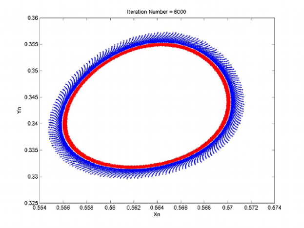
Figure 3: Hopf bifurcation at interior fixed point ($\cong(0.5639,0.3417)$) for $\lambda=0.99,\,\mu=4.5449$, with eigenvalues $\xi\cong-0.3889\pm 0.9215i$. The initial points are $(x,y)=(0.555,0.340)$ and $(x,y)=(0.558,0.34)$.

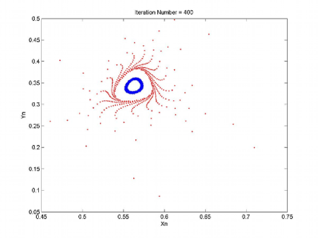
Figure 4: Multiring structure around interior fixed point ($\cong(0.5639,0.3417)$) for $\lambda=0.99,\,\mu=4.55$, with eigenvalues $\xi\cong-0.3903\pm 0.922i$. The initial points are $(x,y)=(0.555,0.338)$ and $(x,y)=(0.43,0.38)$.

5 Chaotic Dynamics and Instability

As pointed out in Theorem 4.2, our model exhibits chaotic dynamics at the limit of the cascade of doubling bifurcations described therein. The proof of this “limiting form” of chaos turns out to be rather subtle and difficult, so we shall not go into it here. Instead, we shall prove the existence of chaotic regimes for higher parameter values using a fairly simple geometric argument based upon demonstrating that a sufficiently high power (iterate) of our model map exhibits Smale horseshoe-like behavior (see e.g. [9, 16, 22, 26]), as illustrated in Fig. 5, and also heteroclinic cycles with transverse intersections (cf. [2, 22, 26]). We keep the value of $\lambda=0.99$, and set $\mu=5$, and summarize our main findings on chaos in the following result.

Theorem 5.1. Let $\Phi:=\Phi_{0.99,5}$. Then there exist an $N\in\mathbb{N}$ and a region $Q$ homeomorphic with a square that intersects the triangular domain $T$, and has the following properties depicted in Fig. $5$:

• $F:=\Phi^{N}$ maps $Q$ onto a pill shaped region, which contains the fixed point $(1,0)$ in its interior, lies along the vertical edge $e_{v}$ of $T$, has maximum $y$ value of $0.22$, and is of sufficient height to include the line segment from $(1,0)$ to $(1,0.2)$ in its interior.

• $G:=\Phi^{N+1}$ maps $Q$ along the curve described above in (B4) into a thin curved homeomorph $\Phi(F(Q))$ of a square that just crosses the diagonal edge $e_{d}$ of $T$ in the interior of the unit square.

• $H:=\Phi^{N+2}=\Phi\circ G$ maps $Q$ into a stretched and folded homeomorph of $Q$ that (transversely) intersects $Q$ in a disjoint pair of curvilinear rectangles in a horseshoe-like fashion.

Consequently, $Q$ contains a compact invariant set $\Lambda$ on which $H$ is topologically conjugate to a shift map $($or equivalently, $\Phi$  is topologically conjugate to a subshift$),$ which implies that $\Phi$ generates chaotic dynamics in $Q\cap\Lambda$, including a dense orbit and cycles of arbitrarily large period.

Proof. We begin our proof with a disk $D$ with an elliptical boundary having its center at $(0.95,0.1)$, semimajor axis length equal to $0.13$ and semiminor axis length equal to $0.075$. Then it follows from the properties of the model map delineated in (B1)-(B5) above that there exist a sufficiently large positive integer $N$ and a diffeomorph of $D$, which we denote as $Q$, such that $\Phi^{-N}(D)=Q$, where $Q$ contains the horizontal edge $e_{h}$ of  $T$ as shown in Fig. 5(a). Observe here that $\Phi$ restricted to $e_{h}$ is a doubling map taking the left vertex into the right vertex, which is symmetric with respect to $x=1/2$, so the inverse notation in this definition must be viewed in the set theoretical preimage context. Nevertheless, $Q$ satisfies $F(Q):=\Phi^{N}(Q)=D$.

Next, we consider the image of $D$ under $\Phi$; namely, $\Phi(D)=\Phi\left(F(Q)\right)=G(Q)$, which is illustrated in Fig. 5(b). To see that this is an accurate depiction of the image, first observe that for the point $(1,0.2)$ lying in the interior of $D$ near its highest point, we have $\Phi(1,0.2)=(0.8,0.8)$, which lies on the diagonal edge $e_{d}$ of $T$. Moreover, the fixed point $(1,0)$ is also an interior point of $D$, but one that lies near its lowest point. Accordingly in virtue of the properties of $\Phi$ - in particular (B4) - the shape of $\Phi(D)$ must be that of the thickened version of part of the parabolic curve described in (B4) and must slightly overlap $e_{d}$ around the point $(0.8,0.8)$, just as depicted in Fig. 5(a).

In order to obtain the desired horseshoe-like behavior, another application of $\Phi$ is required; that is, we need to describe $\Phi^{2}(D)=\Phi\left(G(Q)\right)=H(Q)$. Taking into account the overall definition of the map, property (B3), and the fact that $\Phi(0.8,0.8)=(0.2016,0)$, it is clear that Fig. 4(c) is a rather accurate rendering of the region $H(Q)$, which intersects $Q$ in a fairly typical horseshoe type set comprised of two approximately rectangular components. With this geometric representation of $Q$ and its image $H(Q)$ in hand, we can describe the key fractal component $\Lambda$ of nonwandering set $\Omega$ of $H$ (and a fortiori, $\Phi$) and the topological conjugacy of the restriction of $H$ on $\Lambda$, which we denote as $h$, to a shift map on doubly-infinite binary sequences in essentially the usual way (cf. [9, 16, 22, 26]), modulo a minor alteration necessitated by the fact that $\Phi$ fails to injective on some subsets of $T$.

It remains to describe the alteration and the final steps in defining $\Lambda$ and establishing the topological conjugacy between $h:\Lambda\rightarrow\Lambda$ and the shift map $\sigma:2^{\mathbb{Z}}\rightarrow 2^{\mathbb{Z}}$, where $2^{\mathbb{Z}}:=\{0,1\}^{\mathbb{Z}}$ - the space of all doubly-infinite binary sequences $\ldots a_{-2}a_{-1}a_{0}a_{1}a_{2}\ldots$with $a_{i}=0$ or $1$. To this end, we define $C_{\ell}$ and $C_{r}$ to be the left and right components of $H(Q)\cap Q$, respectively, as shown in Fig. 5(c), and observe that $C_{\ell}\subset Q_{l}:=Q\cap\{(x,y):x<2/5\}$ and $C_{r}\subset Q_{r}^{+}:=\left(Q\cap\{(x,y):x>3/5\}\right)\cup D$. It follows readily from the definition and properties of $\Phi$ delineated in Section 2 that by making $Q$ more slender and $N$, larger, if necessary, $\Phi$ maps $Q_{\ell}$ and $Q_{r}^{+}$ diffeomorphically onto their images, with $\Phi\left(Q_{\ell}\right),\Phi\left(Q\cap\{(x,y):x>3/5\}\right)\subset$ $\{(x,y):x>3/5\}$. In addition, possibly after another shrinking of $Q$ and increase of $N$, we may assume that the iterated sets $\{C_{\ell},\Phi^{m}\left(C_{\ell}\right)\cap Q_{r}^{+}:m\in\mathbb{N}\}$ are pairwise disjoint. We denote the restriction of $\Phi$ to $Q_{\ell}$ and $Q_{r}$ by $\Phi_{\ell}$ and $\Phi_{r}$, respectively. Furthermore, $C_{\ell}$ is the diffeomorphic image of a disjoint set $C_{\ell}^{-1}$ ($=\Phi_{\ell}^{-1}(C_{\ell})$) under $\Phi$, which intersects the edge $e_{d}$, and $C_{\ell}^{-1}$ is, in turn, the diffeomorphic image under $\Phi_{r}$ of a set $C_{\ell}^{-2}$ ($=\Phi_{r}^{-1}(C_{\ell}^{-1})$) contained in $D=\Phi^{N}(Q)$.

We can now define a unique inverse on $\Lambda\subset C_{\ell}\cup C_{r}$ - a set to be defined in this last phase of our proof. As $H^{-1}=\Phi^{-1}\circ\Phi^{-1}\circ\cdots\circ\Phi^{-1}$ ($N$ factors), it remains to select the proper branch of each of the factors in this composition so as to prescribe $H^{-1}$ unambiguously. It is easy to see that this is accomplished as follows: set

$$\Phi_{\ast}^{-1}\left(x,y\right):=\left\{\begin{array}[c]{cc}\Phi_{\ell}^{-1}(x,y),&\left(x,y\right)\in C_{\ell}\cup\Phi_{\ell}\left(C_{\ell}\right)\\ \Phi_{r}^{-1}(x,y)&(x,y)\in C_{\ell}^{-1}\cup\left(Q_{r}^{+}\smallsetminus\Phi_{\ell}\left(C_{\ell}\right)\right)\end{array}\right.,$$

and

$$H^{-1}:=\Phi_{\ast}^{-1}\circ\Phi_{\ast}^{-1}\circ\cdots\circ\Phi_{\ast}^{-1}\quad(N\text{ factors}),$$

and define

$$\Lambda:=Q\cap\left[{\displaystyle\bigcap\nolimits_{m\in\mathbb{Z}}}H^{m}\left(H(Q)\cap Q\right)\right].$$

It is easy to verify that $\Lambda$ is a compact, $H$-invariant set, which is homeomorphic with the cartesian product of a pair of 2-component Cantor sets that , in turn, is homeomorphic with $2^{\mathbb{Z}}$ employing the standard topologies. Then the restriction $h:=H_{\mid\Lambda}$ can be shown to be topologically conjugate to the shift map in the usual way (such as in [9, 22, 26]), thereby completing the proof. $\blacksquare$

We note here that the existence of chaotic regimes described in Theorem 5.1 could also have been demonstrated following a more detailed analysis of the iterates along the lines of the above proof - revealing both transverse homoclinic points of periodic points and transverse heteroclinic points of branches of heteroclinic cycles of periodic points, both of which imply the existence of chaos (as shown or indicated in [2, 9, 16, 22, 26]). The chaotic case (with its characteristic splattering effect) is depicted in Fig. 6, which shows the iterates corresponding to three initial points selected near $(1,0)$. Note the accumulation of points near $(0.85,0)$, $(0.7,0.6)$, $(0.4,0.4)$ and $(0.35,0)$, which are near the set $\Lambda$ and its images under $\Phi$, as described above. Three initial points were used in order to get a reasonable representation of the chaotic iterates because of the sensitivity (associated with chaos) of the system and the limits of computing accuracy.

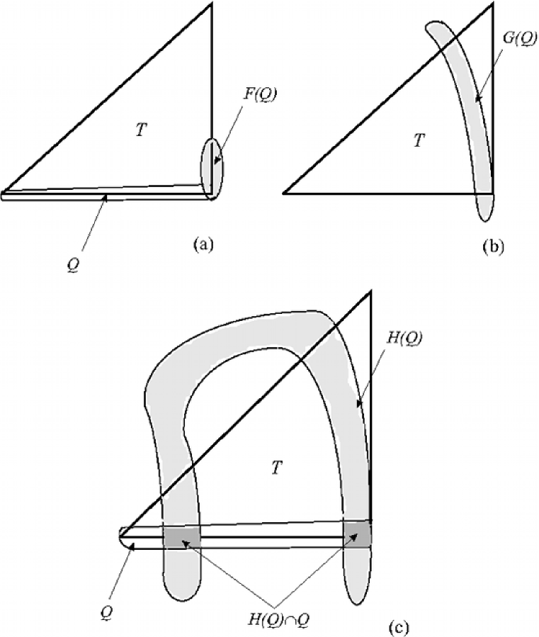
Figure 5: Horseshoe-like behavior of map for $\lambda=0.99,\,\mu=5$: (a) Domain and first stage of geometric image of iterated map; (b) Second stage focusing on stretching and nascent folding; and (c) Final stage of horseshoe configuration

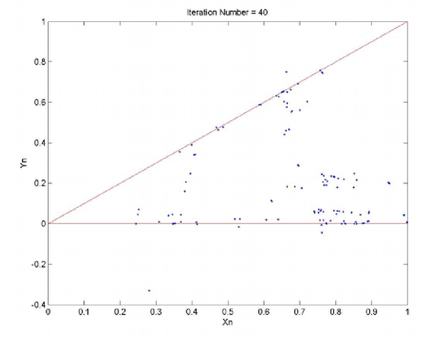
Figure 6: Chaotic orbits about interior fixed point ($\cong(0.5569,0.3569)$) for $\lambda=0.99,\,\mu=4.55$, with eigenvalues $\xi\cong-0.5144\pm 0.9596i$. The three initial points were taken very close to $(1,0)$

6 Comparison with Physical Models

Our purpose in this section is to show that our discrete dynamical model shares many properties with actual physical realizations (and their associated mathematical models) of the R-S flip-flop circuit. Among the several physically based studies of flip-flop type circuit behavior, which includes the work in [4, 8, 14, 15, 17, 19, 20, 21, 23, 27], perhaps the best source of comparison is provided by the investigation of Okazaki et al. [21], so this shall be our focus here. We shall also provide additional numerical simulation illustrations of the behavior of the orbits of our system to further highlight the areas of agreement between our dynamical model and that of [21].

The approach in [21] is quite different from ours. Okazaki and his collaborators start with a physical realization of an R-S flip-flop circuit using two capacitors, one inductor, one linear resistor, one DC battery and a pair of piecewise linear resistors comprised of tunnel diodes. They then derive the state equations for their circuit (hereafter referred to as the OKT system), which is a system of three first-order, piecewise linear ordinary differential equations in two dependent voltage and one dependent current variable, and depends on several parameters associated with the various electrical elements in the circuit. In their study they find numerical solutions of this system of equations using a Runge-Kutta scheme, which they compare with data collected directly from the physical circuit using fairly standard electronic measuring and representation devices. They find that the dynamical behavior deduced from numerical simulation of their system of differential equations is in very good agreement with that observed experimentally from the physical circuit. This behavior includes Hopf bifurcation and chaotic dynamics for certain ranges of their parameters , which of course we have also observed and actually proved for our discrete dynamical model.

More specifically, they deduce - mainly by observing the phase space behavior of their numerical solutions - that there is a certain parameter value where their system develops a Hopf bifurcation on a center manifold, followed, as the parameter increases, by what appears to be a sequence of Hopf bifurcations on the periodic orbits generated. This, of course, is consistent with the qualitative behavior for our model described in Theorems 4.1 and 5.1, and illustrated in Figs. 3 and 4. Moreover, although there are one-dimensional but no two-dimensional Poincaré sections studied in [21], several projections of phase space structure on the two-dimensional voltage coordinate plane, which are at least indicative of Poincaré map behavior on this plane, have a striking similarity to the ring structure delineated in Theorem 5.1. Thus, there appears to be considerable qualitative agreement in the dynamical behavior of our model and the OKT system for parameter values nearly up to but just below those producing full-blown chaos.

Chaotic dynamics for the OKT system [21] is inferred primarily by numerical computation of Lyapunov exponents, analysis of approximate one-dimensional Poincaré sections, and observation of very complicated, ostensibly random outputs in the experimental monitors. The projections onto the voltage coordinate planes also have a somewhat chaotic appearance, with a complicated looking tangle of orbits attached to and partially surrounding the ring configuration mentioned above. Comparing this with the dynamics in the examples pictured in Fig. 5 and 6, which shows ring configurations and the tell-tale splatter (around the rings and concentrated near the fixed point) associated with chaotic discrete dynamics, we have additional qualitative validation for our model.

7 Concluding Remarks

In this investigation we have introduced and analyzed a rather simple discrete dynamical model for the R-S flip-flop circuit, which is based upon the iterates of a two-parameter family of planar, quadratic maps. We proved that for certain parameter ranges, the dynamics of our model exhibits the qualitative behavior expected in and observed for physical realizations of the logical R-S flip-flop circuit such as Hopf bifurcations and chaotic responses including oscillatory outputs of arbitrarily large periods concentrated around states corresponding to nearly equal set and reset inputs. In addition, we indicated how the dynamics of our model displays fascinating complexity - as the parameters are varied - generated by cascading bifurcations of stability transferring, doublings of invariant collections of curves encircling a single equilibrium state, which produce extremely intricate orbit structures.

Not being satisfied with the fact that the interesting variety of complex dynamical structures produced by our model is certainly interesting from a purely mathematical perspective, we undertook a more comprehensive validation by comparing our results with the numerically simulated and experimentally observed characteristics of a fairly standard realization of an R-S flip-flop circuit comprised of linear elements such as inductors and capacitors and piecewise linear components consisting of tunnel diodes. We found that the qualitative agreement between the dynamics of our model and that of physical realization is surprisingly good. Notwithstanding this very favorable comparison, we are aware that it may be largely fortuitous. After all, our model is formulated in an essentially ad hoc manner that relies heavily on intuition and a desire to obtain the simplest maps producing the kinds of dynamics known to be exhibited in working R-S flip-flop circuits. Consequently, we are in the near future going to revisit this logical circuit and investigate others of its kind using a much more direct, first principles oriented approach along the lines of the work of Danca [8] and Hamill et al. [10]. Of course, it would be particularly satisfying if we are able to show that such an approach produces essentially the same discrete model for the R-S flip-flop circuit investigated here, which is something that we expect but naturally remains to be seen. We also intend to formulate and prove a generalized version of Theorem 5.1, which we expect to have numerous applications in our envisaged program of developing discrete dynamical models for a host of logical circuits.

References

- [1] V. Arnold, Small denominators, I: mappings of the circumference into itself, AMS Transl. Ser. 2 46 (1965), 213-284.
- [2] D. Blackmore, New models for chaotic dynamics, Regular & Chaotic Dynamics 10 (2005), 307-321.
- [3] J. Champanerkar and D. Blackmore, Pitchfork bifurcations of invariant manifolds, Topology and Its Applications 154 (2007), 1650-1663.
- [4] T. Chaney, A note on synchronizer and interlock maloperation, IEEE Trans. Computers C-28 (1979), 802-804.
- [5] L. Chua, Chua’s circuit: Ten years later, IEICE Trans. Fundamentals E77-A (1994), 1811-1821.
- [6] L. Chua, C.-W. Wu, A. Huang and G.-Q. Zhong, A universal circuit for studying and generating chaos - Part II: Strange attractors, IEEE Trans. Circuits & Systems 40 (1993), 745-761.
- [7] M. D’Amico, J. Moiola and E. Paolini, Hopf bifurcation in discrete-time systems via a frequency domain approach, Proc. IEEE COC Conf., St. Petersburg, Russia, 2000, pp. 290-293.
- [8] M-F. Danca, Numerical approximation of a class of switch dynamical systems, Chaos, Solitons & Fractals 38 (2008), 184-191.
- [9] J. Guckenheimer and P. Holmes, Nonlinear Oscillations, Dynamical Systems, and Bifurcations of Vector Fields, Springer-Verlag, New York, 1983.
- [10] D. Hamill, J. Deane and D. Jeffries, Modeling of chaotic DC/DC converters by iterated nonlinear maps, IEEE Trans. Power Electron. 7 (1992), 25-36.
- [11] D. Hamill, Learning about chaotic circuits with SPICE, IEEE Trans. Education 36 (1993), 28-35.
- [12] P. Hartman, Ordinary Differential Equations, ed., Birkhäuser, New York, 1982.
- [13] G. Ioos and D. Joseph, Elementary Stability and Bifurcation Theory, Springer-Verlag, New York, 1981.
- [14] T. Kacprzak and A. Albicki, Analysis of metastable operation in RS CMOS flip-flop, IEEE J. Solid-State Circuits SC-22 (1987), 57-64.
- [15] T. Kacprzak, Analysis of oscillatory metastable operation of RS flip-flop, IEEE J. Solid-State Circuits 23 (1988), 260-266.
- [16] A. Katok and B. Hasselblatt, Introduction to the Modern Theory of Dynamical Systems, Cambridge University Press, Cambridge, 1995.
- [17] G. Lacroix, P. Marchegay and N. Al Hossri, Prediction of flip-flop behavior in metastable state, Electron. Lett. 16 (1980), 725-726.
- [18] J. Marsden and M. McCracken, The Hopf Bifurcation and Its Applications, Springer-Verlag, New York, 1976.
- [19] J. Moser, Bistable systems of differential equations with applications to tunnel diode circuits, IBM J. Res. Dev. 5 (1961), 226-240.
- [20] K. Murali, S. Sinha and W. Ditto, Implementation of a nor gate by a chaotic Chua’s circuit, Int. J. Bifurcation and Chaos 13 (2003), 2669-2672.
- [21] H. Okazaki, H. Nakano and T. Kawase, Chaotic and bifurcation behavior in an autonomous flip-flop circuit used by piecewise linear tunnel diodes, IEEE Proc. ?, 1998, III-291 - III-297.
- [22] J. Palis and W. de Melo, Geometric Theory of Dynamical Systems, Springer-Verlag, Berlin, 1982.
- [23] M. Ruzbehani, L. Zhou and M. Wang, Bifurcation features of a dc-dc converter under current-mode control, Chaos, Solitons & Fractals 28 (2006), 205-212.
- [24] Y.H. Wan, Computations of the stability condition for the Hopf bifurcation of diffeomorphisms on , SIAM J. Appl. Math. 34 (1978), 167-175.
- [25] G. Wan, D. Xu and X. Han, On creation of Hopf bifurcations in discrete-time nonlinear systems, CHAOS 12 (2002), 350-355.
- [26] S. Wiggins, Introduction to Applied Nonlinear Dynamical Systems and Chaos, 2nd ed., Springer-Verlag, New York, 2003.
- [27] A. Zorin, E. Tolkacheva, M. Khabipov, F.-I. Buchholz and J. Niemeyer, Dynamics of Josephson junctions and single-flux-quantum networks with superconductor-normal-metal junction shunts, Phys. Rev. B 74 (2006), 014508.