Quantum versus classical polarization states: when multipoles count

Abstract

We advocate for a simple multipole expansion of the polarization density matrix. The resulting multipoles are used to construct bona fide quasiprobability distributions that appear as a sum of successive moments of the Stokes variables; the first one corresponding to the classical picture on the Poincaré sphere. We employ the particular case of the $Q$ function to formulate a whole hierarchy of measures that properly assess higher-order polarization correlations.

1 Introduction

Polarization is a fundamental property of light that has received a lot of attention over the years [1]. As polarization is a robust characteristic, relatively simple to manipulate without inducing more than marginal losses, it is not surprising that many experiments at the forefront of quantum optics involve this observable [2].

In classical optics, polarization is elegantly visualized using the Poincaré sphere and is determined by the Stokes parameters. These are measurable quantities that allow for a classification of the states according to a degree of polarization. Furthermore, the formalism can be extended to the quantum domain, where the Stokes parameters become the mean values of the Stokes operators [3].

The classical degree of polarization is just the length of the Stokes vector. This provides a very intuitive picture, but for intricate fields it has serious drawbacks. Indeed, this classical quantity does not distinguish between states having remarkably different polarization properties [4]. In particular, it can be zero for light that cannot be regarded as unpolarized, giving rise to the so-called hidden polarization [5]. All these flaws have prompted some alternative measures [6, 7, 8, 9, 10, 11, 12, 13, 14, 15, 16, 17, 18, 19].

We adhere to the viewpoint that the Stokes measurements ought to be the basic building blocks for any practical approach to polarization. Actually, the aforesaid problems with the classical degree are due to its definition in terms exclusively of first-order moments of the Stokes variables. This may be sufficient for most classical situations, but for quantum fields higher-order correlations might be crucial.

Our goal in this paper is to advance a practical solution to these hurdles. From coherence theory, we learn that a complete description of interference phenomena involves a hierarchy of correlation functions, with classical behavior represented by the first one of those. In the same spirit, we propose to go beyond the first-order description and look for a way to systematically assess higher-order polarization correlations.

For that purpose, we borrow basic ideas from the standard theory of SU(2) quasidistributions [20], but we reinterpret them in terms of multipoles that contain sequential moments of the Stokes variables. The dipole, being just the first-order moment, can be identified with the classical picture, whereas the other multipoles account for higher-order correlations. Finally, we illustrate how the particular instance of the SU(2) $Q$ function can be used as an efficient measure for the quantitative assessment of those fluctuations.

2 Polarization structure of quantum fields

We start with a brief survey of the basic ingredients involved in a proper description of quantum polarization. We assume a monochromatic plane wave, propagating in the $z$ direction, so its electric field lies in the $xy$ plane. We are thus effectively dealing with a two-mode field that can be characterized by two complex amplitude operators, denoted by $\hat{a}_{\mathrm{H}}$ and $\hat{a}_{\mathrm{V}}$, where the subscripts H and V indicate label horizontal and vertical polarization modes. These operators obey the commutation rules $[\hat{a}_{\lambda},\hat{a}_{\mu}^{\dagger}]=\delta_{\lambda\mu}$, with $\lambda,\mu\in\{\mathrm{H},\mathrm{V}\}$.

The use of the Schwinger representation [21]

$$\textstyle\hat{S}_{1}=\frac{1}{2}(\hat{a}_{\mathrm{H}}^{\dagger}\hat{a}_{\mathrm{V}}+\hat{a}_{\mathrm{V}}^{\dagger}\hat{a}_{\mathrm{H}})\,,\qquad\hat{S}_{2}=\frac{i}{2}(\hat{a}_{\mathrm{H}}\hat{a}_{\mathrm{V}}^{\dagger}-\hat{a}_{\mathrm{H}}^{\dagger}\hat{a}_{\mathrm{V}})\,,\qquad\hat{S}_{3}=\frac{1}{2}(\hat{a}_{\mathrm{H}}^{\dagger}\hat{a}_{\mathrm{H}}-\hat{a}_{\mathrm{V}}^{\dagger}\hat{a}_{\mathrm{V}})\,,$$ (2.1)

together with the total number operator $\hat{N}=\hat{a}_{\mathrm{H}}^{\dagger}\hat{a}_{\mathrm{H}}+\hat{a}_{\mathrm{V}}^{\dagger}\hat{a}_{\mathrm{V}}$, will prove very convenient in what follows. In fact, the average of $\mathbf{\hat{S}}=(\hat{S}_{1},\hat{S}_{2},\hat{S}_{3})$ coincides (except for an unimportant factor 1/2) with the classical Stokes vector [3]. Such a numerical factor is inserted to guarantee that $\{\hat{S}_{k}\}$ satisfy the commutation relations of the su(2) algebra

$$[\hat{S}_{k},\hat{S}_{\ell}]=i\epsilon_{k\ell m}\,\hat{S}_{m}\,,\qquad[\hat{N},\hat{S}_{k}]=0\,,$$ (2.2)

where the Latin indices run over $\{1,2,3\}$ and $\epsilon_{k\ell m}$ is the Levi-Civita fully antisymmetric tensor. This noncommutability precludes the simultaneous exact measurement of the physical quantities they represent, which is expressed by the uncertainty relation

$$\Delta^{2}\hat{\mathbf{S}}=\Delta^{2}\hat{S}_{1}+\Delta^{2}\hat{S}_{2}+\Delta^{2}\hat{S}_{3}\geq\langle\hat{N}\rangle/2\,,$$ (2.3)

$\Delta^{2}\hat{S}_{k}=\langle\hat{S}_{k}^{2}\rangle-\langle\hat{S}_{k}\rangle^{2}$ standing for the variance.

In classical optics, the states of definite polarization are specified by the constraint $\langle\hat{\mathbf{S}}\rangle^{2}=\langle\hat{N}/2\rangle^{2}$. Since the intensity is there a nonfluctuating quantity, in the three-dimensional space of the Stokes parameters this define a sphere with radius equal to the intensity: the Poincaré sphere. In contradistinction, in quantum optics we have that $\hat{\mathbf{S}}^{2}=S(S+1)\leavevmode\hbox{\small 1\normalsize\kern-3.30002pt1}$, with the angular momentum being $S=N/2$ and, as fluctuations in the number of photons are unavoidable, we are forced to work in the three-dimensional Poincaré space that can be regarded as a set of nested spheres with radii proportional to the different photon numbers that contribute to the state.

As our final remark, we stress that the second equation in (2.2) prompts to address each subspace with fixed number of photons $N$ separately. To bring this point out more clearly, it is advantageous to relabel the standard two-mode Fock basis $|n_{\mathrm{H}},n_{\mathrm{V}}\rangle$ in the form

$$|S,m\rangle=|n_{\mathrm{H}}=S+m,n_{\mathrm{V}}=S-m\rangle\,,$$ (2.4)

so that $S=N/2$ and $m=(n_{H}-n_{V})/2$. For each fixed $S$, $m$ runs from $-S$ to $S$ and the states (2.4) span a $(2S+1)$-dimensional subspace wherein $\hat{\mathbf{S}}$ act in the standard way.

3 The polarization sector

For any arbitrary function of the Stokes operators $f(\hat{\mathbf{S}})$, we have $[f(\hat{\mathbf{S}}),\hat{N}]=0$ as well, so the matrix elements of the density matrix $\hat{\varrho}$ connecting subspaces with different photon numbers do not contribute to $\langle f(\hat{\mathbf{S}})\rangle$. This translates the fact that polarization and intensity are, in principle, independent concepts: in classical optics the form of the ellipse traced out by the electric field (polarization) does not depend on its size (intensity).

In other words, the only accessible information from $\hat{\varrho}$ is its polarization sector [22, 23, 24, 25, 26], which is specified by the block-diagonal form

$$\hat{\varrho}_{\mathrm{pol}}=\bigoplus_{S}\hat{\varrho}^{(S)}$$ (3.1)

where $\hat{\varrho}^{(S)}$ is the reduced density matrix in the $S$th subspace ($S$ runs over all the possible photon numbers, i. e., $S=1/2,1,\ldots$). Any $\hat{\varrho}$ and its associated block-diagonal form $\hat{\varrho}_{\mathrm{pol}}$ cannot be distinguished in polarization measurements; accordingly, we drop henceforth the subscript pol.

To go ahead, we resort to the standard SU(2) machinery [27] and expand each $\hat{\varrho}^{(S)}$ as

$$\hat{\varrho}^{(S)}=\sum_{K=0}^{2S}\sum_{q=-K}^{K}\varrho_{Kq}^{(S)}\,\hat{T}_{Kq}^{(S)}\,,$$ (3.2)

where the irreducible tensor operators $\hat{T}_{Kq}^{(S)}$ (please, note carefully that the index $K$ takes only integer values) read [28]

$$\hat{T}_{Kq}^{(S)}=\sqrt{\frac{2K+1}{2S+1}}\sum_{m,m^{\prime}=-S}^{S}C_{Sm,Kq}^{Sm^{\prime}}\,|S,m^{\prime}\rangle\langle S,m|\,,$$ (3.3)

and the expansion coefficients

$$\varrho_{Kq}^{(S)}=\Tr[\hat{\varrho}^{(S)}\,T_{Kq}^{(S)\,\dagger}]$$ (3.4)

are known as state multipoles and contain all the information about the state. The quantities $C_{Sm,Kq}^{Sm^{\prime}}$ are the Clebsch-Gordan coefficients that couple a spin $S$ and a spin $K$ to a total spin $S$ and vanish unless the usual angular momentum coupling rules are satisfied, namely

$$0\leq K\leq 2S\,,\qquad-K\leq q\leq K\,.$$ (3.5)

The operators $\hat{T}_{Kq}^{(S)}$ are quite a convenient tool for they have the proper transformation properties under rotations and besides fulfill

$$\Tr[T_{Kq}^{(S)\,\dagger}\,T_{K^{\prime}q^{\prime}}^{(S)}]=\delta_{KK^{\prime}}\delta_{qq^{\prime}}\,,$$ (3.6)

so, they indeed constitute the most suitable orthonormal basis for the problem at hand. Although the definition of $\hat{T}_{Kq}^{(S)}$ in (3.3) might look a bit unfriendly, the essential observation for what follows is that $\hat{T}^{(S)}_{Kq}$ can be related to the $K$th power of the generators (2.1), so they are intimately linked to the moments of the Stokes variables, precisely our main objective in this work. In particular, the monopole $\varrho_{00}^{(S)}$ being proportional to the identity, is always trivial, while the dipole $\varrho_{1q}^{(S)}$ is the first-order moment of $\hat{\mathbf{S}}$ and thus gives the classical picture, in which the state is represented by its average value.

The complete characterization of the state demands the knowledge of all the multipoles. This implies measuring the probability distribution of $\hat{\mathbf{S}}$ in all the directions, and then performing an integral inversion (put in another way, a whole tomography), which turns out to be a hard task [24, 25, 26]. However, in most realistic cases, only a finite number of multipoles are needed and then the reconstruction of the $K$th multipole entails measuring along just $2K+1$ independent directions [29, 30].

4 Polarization quasidistributions

The discussion thus far suggests that polarization must be specified by a probability distribution of polarization states. As a matter of fact, such a probabilistic description is unavoidable in quantum optics from the very beginning, since $\{\hat{S}_{k}\}$ do not commute and thus no state can have a definite value of all them simultaneously.

The SU(2) symmetry inherent in the polarization structure, as discussed in the previous sections, allows us to take advantage of the pioneering work of Stratonovich [31] and Berezin [32], who worked out quasiprobability distributions on the sphere satisfying all the pertinent requirements. This construction was later generalized by others [33, 34, 35, 36, 37] and has proved to be very useful in visualizing properties of spinlike systems [38, 39, 40, 41, 42].

For each partial $\hat{\varrho}^{(S)}$, one can define the SU(2) $Q$ function as

$$Q^{(S)}(\theta,\phi)=\langle S;\theta,\phi|\hat{\varrho}^{(S)}|S;\theta,\phi\rangle\,,$$ (4.1)

where $|S;\theta,\phi\rangle$ are the SU(2) coherent states (also known as spin or atomic coherent states), given by [43, 44]

$$|S;\theta,\phi\rangle=\hat{D}(\theta,\phi)|S,-S\rangle\,.$$ (4.2)

Here $\hat{D}(\theta,\phi)=\exp(\xi\hat{S}_{+}-\xi^{\ast}\hat{S}_{-})$ [with $\xi=(\theta/2)\exp(-i\phi)$ and $(\theta,\phi)$ being spherical angular coordinates] plays the role of a displacement on the Poincaré sphere of radius $S$. The ladder operators $\hat{S}_{\pm}=\hat{S}_{1}\pm i\hat{S}_{2}$ select the fiducial state $|S,-S\rangle$ as usual: $\hat{S}_{-}|S,-S\rangle=0$. As we can appreciate, both the definition of the $Q$ function and the coherent states for SU(2) closely mimic their standard counterparts for position-momentum.

While for spins, $S$ is typically a fixed number, in quantum optics most of the states involve a full polarization sector as in equation (3.1) and for the total polarization matrix $\hat{\varrho}$ we have

$$Q(\theta,\phi)=\sum_{S}\frac{2S+1}{4\pi}Q^{(S)}(\theta,\phi)\,.$$ (4.3)

The sum extends over the subspaces contributing to the state. Since the SU(2) coherent states are eigenstates of the total number operator $\hat{N}$, the sum over $S$ in (4.3) attempts to remove the total intensity of the field in such a way that $Q(\theta,\phi)$ contains only relevant polarization information. Furthermore, since $|S;\theta,\phi\rangle$ are the only states saturating the uncertainty relation (2.3), the definition of $Q(\theta,\phi)$ is quite appealing, for it appears as the projection on the states having the most definite polarization allowed by the quantum theory.

On the other hand, as $Q$ contains the whole information about the state, its knowledge is tantamount to determining all the state multipoles. Actually, the $Q$ function (and, more generally, any $s$-parametrized quasidistribution) can be also written in terms of $\varrho_{Kq}^{(S)}$ [45]:

$$Q^{(S)}(\theta,\phi)=\frac{\sqrt{4\pi}}{\sqrt{2S+1}}\sum_{K=0}^{2S}\sum_{q=-K}^{K}C_{SS,K0}^{SS}\,\varrho_{Kq}^{(S)}\,Y_{Kq}^{\ast}(\theta,\phi)\,,$$ (4.4)

with $Y_{Kq}(\theta,\phi)$ being the spherical harmonics, which constitute a complete set of orthonormal functions on the sphere. This definition can be shown to be fully equivalent to (4.1). Note also that the Clebsch-Gordan coefficient $C_{SS,K0}^{SS}$ has a very simple analytical form [28]:

$$C_{SS,K0}^{SS}=\frac{\sqrt{2S+1}(2S)!}{\sqrt{(2S-K)!\,(2S+1+K)!}}\,.$$ (4.5)

By plugging (4.4) in the general definition (4.3), we can express the $Q$ function as a sum over multipoles:

$$Q(\theta,\phi)=\sum_{K=0}^{\infty}Q_{K}(\theta,\phi)\,,$$ (4.6)

where each partial component can be written as

$$Q_{K}(\theta,\phi)=\sum_{S=\lfloor K/2\rfloor}^{\infty}\sqrt{\frac{2S+1}{4\pi}}\sum_{q=-K}^{K}C_{SS,K0}^{SS}\,\varrho_{Kq}^{(S)}\,Y_{Kq}^{\ast}(\theta,\phi)\,.$$ (4.7)

Here, the floor function $\lfloor x\rfloor$ is the largest integer not greater than $x$. For the particular case of single $S$ (fixed number of photons), the sum over $S$ has to be ignored.

The partial components $Q_{K}$ inherit the properties of $Q$, but they contain exclusively the relevant information of the $K$th moment of the Stokes variables. So, (4.6) appears as an optimum tool to arrange the successive moments and thus achieves our goals in this paper.

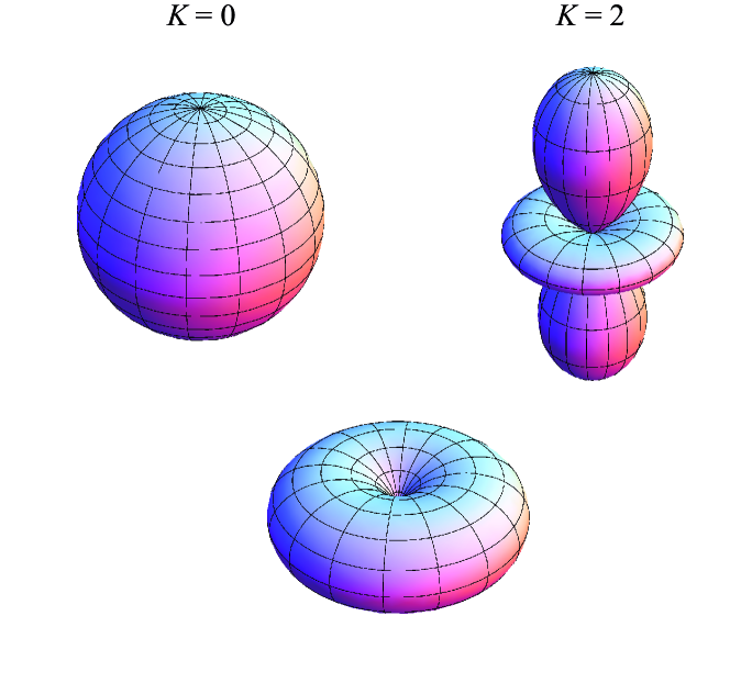
Figure 1: Plot of the monopolar ($K=0$) and quadrupolar ($K=2$) components of the state $|1,0\rangle$ (top), as well as the total $Q$ function (bottom). The dipolar component ($K=1$) vanishes, so this state lacks any first-orden information, which translates in the presence of hidden polarization.

Let us illustrate our viewpoint with the simple example of the state $|1_{\mathrm{H}},1_{\mathrm{V}}\rangle$, produced in parametric down conversion. In the $|S,m\rangle$ notation, the state is $|1,0\rangle$ and its $Q$ function can be easily computed according to (4.6) and (4.7); the final result is

$$Q(\theta,\phi)=\frac{3}{4}\sqrt{\frac{1}{3\pi}}\sin^{2}\theta\,.$$ (4.8)

It does not depend on $\phi$ and its shape is an equatorial belly, revealing that the state is highly delocalized. The partial components are

$$Q_{0}(\theta,\phi)=\frac{1}{2}\sqrt{\frac{1}{3\pi}}\,,\quad Q_{1}(\theta,\phi)=0\,,\quad Q_{2}(\theta,\phi)=-\frac{1}{2}\sqrt{\frac{1}{3\pi}}\left(\frac{3}{2}\cos^{2}\theta-\frac{1}{2}\right)\,.$$ (4.9)

The sum of these three terms gives, of course, the result (4.8), but anyway there is more information encoded in (4.9): the dipole contribution is absent, confirming that this state conveys no first-order information (i.e., is unpolarized to that order). This is the reason why this is the first state in which hidden polarization was detected. Figure 1 shows the partial $Q_{K}$ functions for this state, as well the global one.

5 Assessing higher-order polarization moments

Let us consider the following quantity

$$\mathcal{A}=\int d\Omega\,[Q(\theta,\phi)]^{2}\,,$$ (5.1)

where the integral extends over the whole sphere and $d\Omega=\sin\theta d\theta d\phi$ is the solid angle. This function can be interpreted as the effective area where the $Q$ function is different from zero. Similar proposals have already been used as measures of localization and uncertainty in different contexts [46, 47, 48, 49, 50, 51]. In polarization, (5.1) has been also used as an essential ingredient in formalizing an alternative degree arising as the distance between the state’s $Q$ function and the $Q$ function for unpolarized light [6].

One might think the use of the Wigner function preferable as a measure of the area occupied by a quantum state in phase space. However, for SU(2) $\int d\Omega[W(\theta,\phi)]^{2}$ takes exactly the same value for all pure states, so that this provides a measure of purity of quantum states rather than a measure of polarization. For this compelling reason, we have instead employed the $Q$ function so far.

Note that (5.1) is invariant under SU(2) transformations: this means that such an effective area depends on the form of the $Q$ function, but not on its position or orientation on the Poincaré sphere.

Of course, the decomposition in multipoles (4.6) is of straightforward application here. Consequently, we can define the magnitude

$$\mathcal{A}_{K}=\int d\Omega\,[Q_{K}(\theta,\phi)]^{2}\,,$$ (5.2)

with an analogous interpretation to that $\mathcal{A}$, but restricted to the $K$th multipole. Let us restrict ourselves to a fixed $S$ (and drop the corresponding superscript for clarity); the generalization for a sum of $S$s is direct. When the explicit form of $Q_{K}$ in (4.7) is used, $\mathcal{A}_{K}$ reduces to

$$\mathcal{A}_{K}=\sum_{S=\lfloor K/2\rfloor}^{\infty}\frac{2S+1}{4\pi}\sum_{q=-K}^{K}\left(C_{SS,K0}^{SS}\right)^{2}|\varrho_{Kq}^{(S)}|^{2}\,.$$ (5.3)

In this way, $\mathcal{A}_{K}$ can be reinterpreted as a measure of the strength of the corresponding multipole, confirming that it provides full information about the state $K$th moment.

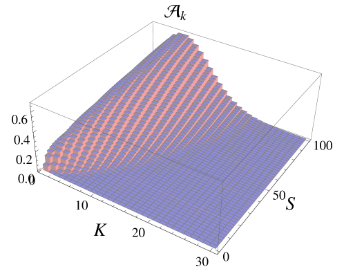
Figure 2: Function $\mathcal{A}_{K}$ as a function of the multipole order $K$ for a SU(2) coherent state for different values of $S$.

As an appealing illustration of our method, we analyze the outstanding example of SU(2) coherent states. Without lack of generality, we deal with the south pole $|S,-S\rangle$, since from (4.2) any other coherent state can be obtained by the application of a displacement to that state. The associated multipoles turn out to be $\varrho_{Kq}^{(S)}=\sqrt{(2K+1)/(2S+1)}C_{SS,K0}^{SS}$, so that

$$\mathcal{A}_{K}=\frac{2K+1}{4\pi}\left(C_{SS,K0}^{SS}\right)^{4}\,.$$ (5.4)

In figure 2 we have plotted $\mathcal{A}_{K}$ as a function of $K$ and $S$. The first multipoles contribute always the most to the state localization, something that one could expect from physical intuition. However, as $S$ gets larger, the number of multipoles to take into account also increases.

6 Concluding remarks

Multipolar expansions are a commonplace and a powerful tool in many branches of physics. We have applied such an expansion to the polarization density matrix, showing how the corresponding state multipoles represent higher-order correlations in the Stokes variables. This paves the way to a systematic characterization of quantum polarization fluctuations that, paradoxically, is still missing in the realm of quantum optics. Such a complete programme is presently in progress in our group.

References

- [1] Brosseau C 1998 Fundamentals of Polarized Light: A Statistical Optics Approach (New York: Wiley)
- [2] Mandel L and Wolf E 1995 Optical Coherence and Quantum Optics (Cambridge: Cambridge University Press)
- [3] Luis A and Sánchez-Soto L L 2000 Quantum phase difference, phase measurements and Stokes operators (Progress in Optics vol 41) (Amsterdam: Elsevier) pp 421–481
- [4] Tsegaye T, Söderholm J, Atatüre M, Trifonov A, Björk G, Sergienko A V, Saleh B E A and Teich M C 2000 Phys. Rev. Lett. 85 5013–5017
- [5] Klyshko D N 1992 Phys. Lett. A 163 349–355
- [6] Luis A 2002 Phys. Rev. A 66 013806
- [7] Legré M, Wegmüller M and Gisin N 2003 Phys. Rev. Lett. 91 167902
- [8] Saastamoinen T and Tervo J 2004 J. Mod. Opt. 51 2039–2045
- [9] Picozzi A 2004 Opt. Lett. 29 1653–1655
- [10] Ellis J, Dogariu A, Ponomarenko S and Wolf E 2005 Opt. Commun. 248 333–337
- [11] Luis A 2005 Phys. Rev. A 71 053801
- [12] Sehat A, Söderholm J, Björk G, Espinoza P, Klimov A B and Sánchez-Soto L L 2005 Phys. Rev. A 71 033818
- [13] Klimov A B, Sánchez-Soto L L, Yustas E C, Söderholm J and Björk G 2005 Phys. Rev. A 72 033813
- [14] Réfrégier P 2005 Opt. Lett. 30 1090–1092
- [15] Réfrégier P and Goudail F 2006 J. Opt. Soc. Am. A 23 671–678
- [16] Luis A 2007 Opt. Commun. 273 173–181
- [17] Björk G, Söderholm J, Sánchez-Soto L L, Klimov A B, Ghiu I, Marian P and Marian T A 2010 Opt. Commun. 283 4440–4447
- [18] Klimov A B, Björk G, Söderholm J, Madsen L S, Lassen M, Andersen U L, Heersink J, Dong R, Marquardt C, Leuchs G and Sánchez-Soto L L 2010 Phys. Rev. Lett. 105 153602
- [19] Qian X F and Eberly J H 2011 Opt. Lett. 36 4110–4112
- [20] Varilly J C and Gracia-Bondía J M 1989 Ann. Phys. 190 107–148
- [21] Schwinger J 1965 On angular momentum Quantum Theory of Angular Momentum ed Biedenharn L C and Dam H (New York: Academic)
- [22] Karassiov V P 1993 J. Phys. A 26 4345–4354
- [23] Raymer M G, McAlister D F and Funk A 2000 Measuring the quantum polarization state of light Quantum Communication, Computing, and Measurement 2 ed Kumar P (New York: Plenum)
- [24] Karassiov V P and Masalov A V 2004 JETP 99 51–60
- [25] Marquardt C, Heersink J, Dong R, Chekhova M V, Klimov A B, Sánchez-Soto L L, Andersen U L and Leuchs G 2007 Phys. Rev. Lett. 99 220401
- [26] Müller C R, Stoklasa B, Peuntinger C, Gabriel C, Řeháček J, Hradil Z, Klimov A B, Leuchs G, Marquardt C and Sánchez-Soto L L 2012 New J. Phys. 14 085002
- [27] Blum K 1981 Density Matrix Theory and Applications (New York: Plenum)
- [28] Varshalovich D A, Moskalev A N and Khersonskii V K 1988 Quantum Theory of Angular Momentum (Singapore: World Scientific)
- [29] Newton R G and Young B l 1968 Ann. Phys. 49 393–402
- [30] Klimov A B, Björk G, Müller C, Leuchs G and Sánchez-Soto L L 2012 To be published
- [31] Stratonovich R L 1956 JETP 31 1012—1020
- [32] Berezin F A 1975 Commun. Math. Phys. 40 153–174
- [33] Agarwal G S 1981 Phys. Rev. A 24 2889–2896
- [34] Brif C and Mann A 1998 J. Phys. A 31 L9–L17
- [35] Heiss S and Weigert S 2000 Phys. Rev. A 63 012105
- [36] Klimov A B and Chumakov S M 2000 J. Opt. Soc. Am. A 17 2315–2318
- [37] Klimov A B and Romero J L 2008 J. Phys. A 41 055303
- [38] Dowling J P, Agarwal G S and Schleich W P 1994 Phys. Rev. A 49 4101–4109
- [39] Atakishiyev N M, Chumakov S M and Wolf K B 1998 J. Math. Phys. 39 6247–6261
- [40] Chumakov S M, Frank A and Wolf K B 1999 Phys. Rev. A 60 1817–1822
- [41] Chumakov S M, Klimov A B and Wolf K B 2000 Phys. Rev. A 61 034101
- [42] Klimov A B 2002 J. Math. Phys. 43 2202–2213
- [43] Arecchi F T, Courtens E, Gilmore R and Thomas H 1972 Phys. Rev. A 6 2211–2237
- [44] Perelomov A 1986 Generalized Coherent States and their Applications (Berlin: Springer)
- [45] Agarwal G S 1981 Phys. Rev. A 24 2889–2896
- [46] Heller E J 1987 Phys. Rev. A 35 1360–1370
- [47] Maassen H and Uffink J B M 1988 Phys. Rev. Lett. 60 1103–1106
- [48] Anderson A and Halliwell J J 1993 Phys. Rev. D 48 2753–2765
- [49] Hall M J W 1999 Phys. Rev. A 59 2602–2615
- [50] Gnutzmann S and Zyczkowski K 2001 J. Phys. A 34 10123–10140
- [51] Muñoz C, Klimov A B and Sánchez-Soto L L 2012 J. Phys. A 45 244014