Abstract

We study the impact of the measurements of three sets of observables on the parameter space of the constrained minimal supersymmetric Standard Model (cMSSM), its slightly general variant, the non-universal scalar model (NUSM), and some selected benchmark points of the 19-parameter phenomenological MSSM (pMSSM): ($i$) the direct measurement of the Higgs boson mass $m_{h}\approx 125$ GeV at the CERN Large Hadron Collider (LHC); ($ii$) $Z$ boson decay width in the $b\bar{b}$ channel normalized to its hadronic width ($R_{b}$), and the forward-backward asymmetry on the $Z$-peak in the same channel $(A_{\rm FB}^{b})$; and ($iii$) several $B$-physics observables, along with $(g-2)$ of muon. In addition, there are constraints from non-observation of superparticles from direct searches at the LHC. In view of the recently re-estimated standard model (SM) value of $R_{b}$ with improved higher order corrections, the measured value of $R_{b}$ has a 1.2$\sigma$ discrepancy with its SM value, while the corresponding discrepancy in $A_{\rm FB}^{b}$ is 2.5$\sigma$. MSSM contributions from light superpartners improve the agreement of $R_{b}$ but worsen that of $A_{\rm FB}^{b}$. We project this ($R_{b}$-$A_{\rm FB}^{b}$) tension vis-à-vis the constraints arising from other observables in the parameter space of cMSSM and NUSM. We also consider a few well-motivated pMSSM benchmark points and show that pMSSM does not fare any better than the SM.

1 Introduction

It is still premature to conclude that the recently discovered scalar particle with a mass of around 125 GeV at the LHC [1, 2] is the standard model (SM) Higgs boson. Among other possibilities, it can very well be the lightest neutral Higgs boson of the minimal supersymmetric standard model (MSSM), which is the most advocated beyond the SM scenario. Be that as it may, stringent constraints apply on the supersymmetric parameter space, which are, at least for the minimal versions, more severe than those placed from the non-observation of superparticles from direct searches at the colliders. In spite of several advantages that supersymmetry offers, like the solution of the big hierarchy problem and even the provision of a cold dark matter candidate, we cannot escape the following pertinent question: does supersymmetry even partially ease the existing tension between the SM predictions and the experimental measurements for some specific observables? The tension with $(g-2)$ of muon, namely, $\delta a_{\mu}=a_{\mu}^{\rm exp}-a_{\mu}^{\rm SM}=(28.7\pm 8.2)\times 10^{-10}$, i.e. a 3.5$\sigma$ deviation of the measured value [3] from its SM expectation [4, 5], is an old intriguing one. Similarly, there is a longstanding $2.5\sigma$ discrepancy between the SM expectation and the experimental value for the $e^{+}e^{-}\to b\bar{b}$ forward-backward asymmetry $A^{b}_{\rm FB}$ measured on the $Z$-peak [6]. Recently, a 1.2$\sigma$ discrepancy, but with an opposite pull to that of $A^{b}_{\rm FB}$, between the SM prediction and the experimental value for $R_{b}=\Gamma(Z\to b\bar{b})/\Gamma(Z\to{\rm hadrons})$ has been reported following the latest SM calculation taking electroweak two-loop plus order $\alpha\alpha_{S}^{2}$ three-loop effects [7]. Although 1.2$\sigma$ is not statistically too much significant, it is this opposite pull between $R_{b}$ and $A^{b}_{\rm FB}$ that we would like to exploit for discriminating supersymmetric models. Possible ways to ease these hiccups in a model-independent effective theory approach and the corresponding LHC signatures have recently been discussed [8]. But, what these tensions imply for supersymmetric models is the main concern of the present paper.

For definiteness, we will start with the parameter space of the constrained MSSM, called cMSSM, completely specified at the grand unification (GUT) scale by a common scalar mass ($m_{0}$), a common gaugino mass $(M_{1/2})$, a universal scalar trilinear parameter ($A_{0}$), the ratio of the vacuum expectation values of the two Higgs doublets ($\tan\beta$), and the sign of the Higgsino mass parameter ($\mu$) [9, 10]. We place indirect constraints on the cMSSM parameter space from observables classified here under three categories:

1. The lightest CP-even Higgs mass $m_{h}\approx 125$ GeV, reaching out to which requires the stop squarks to be very heavy (several TeV) or having a substantial mixing between their left and right components [11, 12]. Since all superparticle masses are interrelated in terms of the $(4+1)$ GUT scale parameters, the Higgs mass puts by far the strongest constraint on the cMSSM parameter space.

2. A set of $B$-physics observables, namely, ${\rm Br}(b\to s\gamma)$, ${\rm Br}(B_{s}\to\mu^{+}\mu^{-})$, ${\rm Br}(B^{\pm}\to\tau\nu)$, and ${\rm Br}(B\to D^{(*)}\tau\nu)$. The first two processes, being loop-induced in both SM and cMSSM, put a strong constraint on the cMSSM parameters from the fact that the data on them are quite precise and completely consistent with the SM expectations. The new physics parts for the remaining ones are mediated essentially by the charged Higgs boson, and here the data show some intriguing discrepancy with the SM expectations. We include the measurement of $(g-2)$ of muon too in this category, which prefers the smuons and gaugino/higgsino to be light.

3. The $Z$-peak observables $R_{b}$ and $A_{\rm FB}^{b}$. Both are precision electroweak observables, with a pull of 1.2$\sigma$ and 2.5$\sigma$ respectively, when experimental data are compared with their SM predictions. The supersymmetric contributions to these observables in the current context form the core of our analysis.

Constraints from the interplay of the first two categories listed above have already been placed by several authors [13, 14]. The main thrust of the present paper is to explore if it is possible to additionally satisfy the constraints listed in the third category. The electroweak precision data was analyzed vis-à-vis MSSM in Ref. [15], but at a time when the discrepancy between the measured value of $R_{b}$ and the SM one-loop estimate was only about $0.6\sigma$, and the Higgs boson was not discovered. So it is only proper to readdress the issue in the light of the present wisdom, especially when the Higgs boson has finally been observed, and estimate of higher-order effects on $R_{b}$ has widened the discrepancy from $0.6\sigma$ to $1.2\sigma$. Also, the opposite pull between $R_{b}$ and $A_{\rm FB}^{b}$ should be paid due attention, as these are precision observables.

We note that in cMSSM the masses of the squarks and the charged Higgs boson stem from a common $m_{0}$. Therefore, non-observation of squarks in direct searches automatically implies that the charged Higgs boson has to be heavy. For this reason, for some of the $B$-physics observables where the charged Higgs boson contributes as the sole new physics at tree level, its numerical impact is rather suppressed. To liberate the charged Higgs boson from this unfavorable tie-up with the squarks, we consider a slightly wider variant, called the non-universal scalar model (NUSM), which is characterized by two different soft scalar masses at the GUT scale: $m_{16}$ for the matter scalars which belong to a 16-plet, and $m_{10}$ for the Higgs scalars which belong to a decuplet, of the underlying SO(10) [16]. Note that even if there is a common scalar mass at the Planck scale $M_{Pl}$, the matter and Higgs scalar masses at the GUT scale $M_{G}$ can be different because of renormalization group running controlled by a priori unknown physics between $M_{Pl}$ and $M_{G}$. From this perspective, one might take $m_{10}$ and $m_{16}$ as independent parameters. In this case, non-observation of squarks does not necessarily imply that the charged Higgs boson is heavy. Still, the masses of the charged Higgs boson and the squarks in NUSM are not fully uncorrelated because of the radiative corrections to the Higgs mass parameters coming from the stop squarks involving large Yukawa couplings. Even then, we observe that a lot of parameter space in the charged Higgs mass plane which is disfavored in cMSSM is resurrected in NUSM.

In the last part of this paper, we will consider selected benchmark points of the 19-parameter phenomenological MSSM (pMSSM) [18], which is a subspace of pMSSM with parameters defined at the weak scale, without introducing any theoretical prejudice about their high scale behaviors. 24 such benchmark model points have been considered in Ref. [19], which correspond to different regions of the MSSM parameter space, consistent with all other constraints like the Higgs mass, dark matter relic density, and direct searches at the LHC. Out of these 24 model points, 5 have been shortlisted in [19]. We will analyse how these well-motivated benchmark points react to the combined effects of ($R_{b}$–$A_{\rm FB}^{b}$) and a few other observables.

2 ${\mathbf{R_{b}}}$ and ${\mathbf{A_{\rm FB}^{b}}}$

The one-loop corrected $Zb\bar{b}$ coupling, including new physics, can be written as

$${\cal L}_{Zb\bar{b}}=-\frac{g}{\cos\theta_{W}}\bar{b}\gamma^{\mu}\left[(g_{L}^{b}+\delta g_{L}^{b})P_{L}+(g_{R}^{b}+\delta g_{R}^{b})P_{R}\right]bZ_{\mu}\,,$$ (1)

where

$$g_{L}^{b}=\sqrt{\rho_{b}}\left(t_{3}^{b}-\kappa_{b}Q_{b}\sin^{2}\theta_{W}\right)\,,\ \ g_{R}^{b}=-\sqrt{\rho_{b}}\kappa_{b}Q_{b}\sin^{2}\theta_{W}\,,$$ (2)

with $\rho_{b}=0.9869$ and $\kappa_{b}=1.0067$ after incorporating the SM electroweak corrections in the $\overline{\rm MS}$ scheme [6], and $\delta g_{L,R}^{b}$ capture the higher-order effects coming from new physics. Here, $t_{3}^{b}=-\frac{1}{2}$, $Q_{b}=-\frac{1}{3}$, and $P_{L(R)}=\frac{1}{2}(1-(+)\gamma_{5})$. The loop corrections induced by the superparticles can be approximated as

$$\delta g_{L(R)}^{b} = \xi F_{L(R)}\,,~{}~{}~{}{\rm with}~{}~{}\xi=\frac{\alpha}{4\pi\sin^{2}\theta_{W}}\,.$$ (3)

The expressions for the quantities $F_{L}$ and $F_{R}$ have been adapted from Appendix B of Ref. [20]. They contain contributions from top-charged Higgs, stop-chargino and sbottom-neutralino loops, expressed in terms of the Passarino-Veltman functions [21]. The new contribution to $R_{b}$ can be written as

$$\delta R_{b}=R_{b}^{\rm SM}\left(1-R_{b}^{\rm SM}\right)\nabla_{b}\,,$$ (4)

with

$$\nabla_{b}=\xi\left[\frac{2g^{b}_{L}F_{L}+2g^{b}_{R}F_{R}}{\left(g^{b}_{L}\right)^{2}+\left(g^{b}_{R}\right)^{2}}\right]\approx\xi\left[-\frac{60}{13}F_{L}+\frac{12}{13}F_{R}\right]\,,$$ (5)

where the right-most simplified expression in Eq. (5) is shown only for illustration by approximating $\kappa_{b}=1$ and $\sin^{2}\theta_{W}=0.25$. However, this approximation is shown only for illustrative purpose. The full expression in MSSM can be found in [20, 15] which we have employed for our numerical analysis.. The Gfitter group [22] has recently updated the SM fit (after the Higgs discovery) using the improved calculation of $R_{b}$ with the result that the discrepancy with the measured value is now 1.2$\sigma$ [7]. The new situation is the following:

$$R_{b}~{}({\rm exp})=0.21629\pm 0.00066\,,\ \ R_{b}~{}({\rm SM})=0.21550\pm 0.00003\,.$$ (6)

The change in $A^{b}_{\rm FB}$ can similarly be written as

$$\frac{A^{b}_{\rm FB}}{A^{b}_{\rm FB}({\rm SM})}-1=\xi\left[\frac{2g^{b}_{R}F_{R}-2g^{b}_{L}F_{L}}{\left(g^{b}_{R}\right)^{2}-\left(g^{b}_{L}\right)^{2}}-\frac{2g^{b}_{R}F_{R}+2g^{b}_{L}F_{L}}{\left(g^{b}_{R}\right)^{2}+\left(g^{b}_{L}\right)^{2}}\right]\approx-\frac{5}{13}\xi\left[F_{L}+5F_{R}\right]\,,$$ (7)

for which a $2.5\sigma$ discrepancy between the SM and experimental values is known to exist for a while [6]:

$$A^{b}_{\rm FB}~{}({\rm exp})=0.0992\pm 0.0016\,,\ \ {\rm and}\ \ A^{b}_{\rm FB}~{}({\rm SM})=0.1032^{+0.0004}_{-0.0006}\,.$$ (8)

A comparative study of $R_{b}$ and $A^{b}_{\rm FB}$ is now in order. It is not difficult to understand the tension between their supersymmetric contributions irrespective of any other constraints. In MSSM (i.e. not just in cMSSM), both $F_{L}$ and $F_{R}$ turn out to be negative, with $|F_{L}|>|F_{R}|$, because of the presence of the numerically dominant stop-chargino loop contribution for $F_{L}$, which is absent for $F_{R}$. Thus, one can have a consistent solution for $R_{b}$, as can be seen from Eqs. (5) and (6). On the other hand, as Eq. (7) shows, the supersymmetric contribution to $A^{b}_{\rm FB}$ is always positive, while according to Eq. (8) experimental data prefers a negative contribution. Thus, not only cMSSM but a large class of supersymmetric model for which $F_{L},F_{R}<0$ and $|F_{L}|>|F_{R}|$ cannot simultaneously satisfy $R_{b}$ and $A^{b}_{\rm FB}$.

To numerically appreciate the combined effects of $R_{b}$ and $A^{b}_{\rm FB}$, we first define what is known as ‘pull’ for a given observable ($O$), as

$${\rm Pull}=\frac{O_{\rm theory}-O_{\rm expt}}{\sigma_{\rm expt}}\,,$$ (9)

where $O_{\rm expt}$ is the experimental central value and $\sigma_{\rm expt}$ is one standard deviation experimental error. Then we introduce a quantity $X_{b}$ defined as

$$X_{b}=\sqrt{({\rm Pull~{}of}~{}R_{b})^{2}+({\rm Pull~{}of}~{}A^{b}_{\rm FB})^{2}}\,.$$ (10)

Eqs. (6) and (8) tell us that the pulls of $R_{b}$ and $A_{\rm FB}^{b}$ are $-1.2$ and $2.5$, respectively, so that $X_{b}^{\rm SM}=2.8$. Light superparticles can improve the agreement in $R_{b}$, but any such contributions can only worsen the tension in $A^{b}_{\rm FB}$, as explained earlier. Thus $X_{b}$ cannot be smaller than $2.5$. This motivates us to look for the parameter space where $X_{b}$ lies between 2.5 and its SM value 2.8 (which corresponds to completely decoupled supersymmetry). For illustration, we have chosen $X_{b}=2.6$ and 2.7 as two representative values, in the sense that for each case we accept the parameter space which yields $X_{b}$ less than that value. We recall in this context that although $R_{b}$ and $A_{\rm FB}^{b}$ both depend on the dynamics of the $Zb\bar{b}$ vertex, the former is a ratio of decay widths and the latter is an asymmetry, and they are experimentally independent observables. Hence, $X_{b}$ is a good measure of the combined tension produced by these two observables.

3 Results

3.1 cMSSM and NUSM

The model parameters have been scanned in the following range: $0<\left(m_{0},M_{1/2}\right)<2$, $-7<A_{0}<0$ (all in TeV), $10\leq\tan\beta\leq 45$. For the NUSM scenario, we scan over the additional parameter $m_{10}$ in the range of [0:2] TeV. We have used SuSpect2.41 [23] to generate the weak scale spectrum from the high scale boundary values. The package micrOMEGAs2.4 [24] has been utilized to extract observables like branching ratios of $b\to s\gamma$, $B_{s}\rightarrow\mu^{+}\mu^{-}$ and $B^{+}\rightarrow\tau^{+}\nu_{\tau}$. We have used the following experimental ranges for the $B$-physics observables [25, 26], admitting $2\sigma$ spread around their central values, except for ${\rm Br}(B_{d}\to\mu^{+}\mu^{-})$ which is taken at $90\%$ confidence limit:

$${\rm Br}(b\to s\gamma) = (3.55\pm 0.24\pm 0.09)\times 10^{-4}\,,~{}~{}~{}{\rm Br}(B_{s}\to\mu^{+}\mu^{-})=\left(3.2^{+1.5}_{-1.2}\right)\times 10^{-9}\,,$$

$${\rm Br}(B_{d}\to\mu^{+}\mu^{-}) < 0.94\times 10^{-9}\,,~{}~{}~{}{\rm Br}(B^{+}\to\tau^{+}\nu)=(1.15\pm 0.23)\times 10^{-4}\,.$$ (11)

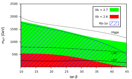
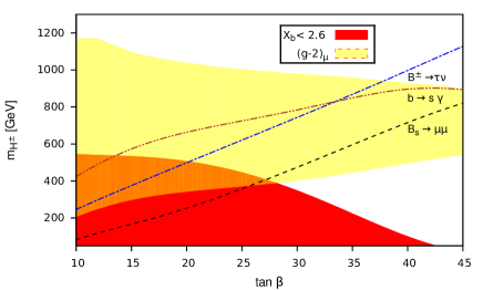
Figure 1: (a) Left panel: Constraints on the $m_{H^{+}}$-$\tan\beta$ plane from $m_{h}=123$ GeV, direct searches of gluinos and squarks at the LHC, and the LEP limit on the chargino mass. The region above each line is allowed. The regions which satisfy $R_{b}$ at $1\sigma$ (blue dashed lines), $X_{b}<2.6$ (red/dark grey patch) and $X_{b}<2.7$ (green/light grey patch) are separately shown. (b) Right panel: Allowed regions from several $B$-physics observables, $(g-2)$ of muon, all taken at $2\sigma$. The red (dark grey) and orange (medium grey) regions satisfy $X_{b}<2.6$, while the yellow (light grey) and orange (medium grey) regions are allowed by $(g-2)$ of muon. For the $B$-physics observables, the region above each line is allowed.

Our results for cMSSM are shown in the left and right panels of Fig. 1 in the plane of the charged Higgs mass and $\tan\beta$. In both panels, we indicate the region which satisfy our criteria for $X_{b}$. In the left panel (a), besides showing the effect of satisfying the Higgs mass, we display the constraints coming from the non-observation of superparticles (mainly, the gluino and the first two generations of squarks) from direct searches at the LHC [27], as well as those originating from the LEP limit on the chargino mass [6]. The region which agrees with $R_{b}$ within 1$\sigma$ is shown by blue dashed lines. While one might argue that a discrepancy of $1.2\sigma$ is not of much significance, we observe that softening the same to even $1\sigma$ requires such light sparticles, in particular the stop squarks, as to be untenable with the Higgs mass constraint. We also show regions which admit $X_{b}<2.6$ (red or dark grey) and $X_{b}<2.7$ (green or light grey). We reiterate that the 2.5$\sigma$ pull in $A_{\rm FB}^{b}$ essentially controls the constraint from $X_{b}$. In the right panel (b), we focus on the zone where constraints from several $B$-physics observables, as well as the region allowed by $(g-2)$ of muon, are prominent. Wherever a single line is drawn for a particular observable, the space above that line is allowed from the corresponding constraint. We make a cautionary remark that these lines separate allowed and disallowed regions where all cMSSM input parameters are marginalized. Admittedly, we have not tried to simultaneously fit all the electroweak observables, however, with such large values of the sparticle masses, it is only natural to expect that the observables already consistent with the SM would not suffer any untenable tension. The zone allowed by $(g-2)$ of muon is shown by yellow patch. The dominant contribution to $(g-2)$ of muon comes when the bino and smuons floating inside the loops are light [28]. We have kept the lightest Higgs boson mass at a conservative value of 123 GeV, allowing for the possibility that higher order radiative corrections may contribute a further 2 to 3 GeV (setting $m_{h}=125$ GeV would result in even tighter constraints). Even then, this rules out more region in the $m_{H}^{+}$ versus $\tan\beta$ plane than the other constraints. The reason is that one requires stop masses as heavy as several TeV and a substantial mixing in the stop mass-squared matrix to yield such a Higgs mass [29]. Among the flavor observables, $b\to s\gamma$ usually provides the strongest constraint [30], because it directly constrains the chargino mass which sits in the lower end of the cMSSM spectrum. The constraint gets more stringent at large $\tan\beta$ because the dominant chargino-stop loop amplitude grows as $1/\cos^{2}\beta$. The supersymmetric contribution to the branching ratio of $B_{s}\to\mu^{+}\mu^{-}$ grows as $(\tan\beta)^{6}$ [31], and therefore at large $\tan\beta$ the constraint is more stringent. As regards the process $B^{+}\to\tau^{+}\nu$, the dominant new physics contribution comes from tree-level charged Higgs mediation, and for very large $\tan\beta$ provides a stronger constraint than ${\rm Br}~{}(b\to s\gamma)$. The constraint essentially applies on the ratio $\tan\beta/m_{H^{+}}$, which is a general feature of any two-Higgs doublet model [32].

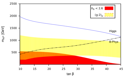
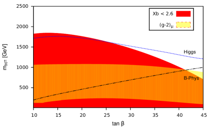
Figure 2: A comparison of constraints between cMSSM (left panel) and NUSM (right panel) arising from the Higgs mass, $(g-2)$ of muon, the combined $B$-physics data, and the requirement of satisfying $X_{b}<2.6$. The color codes are the same as in Fig. 1.

In Fig. 2, we compare cMSSM (left panel) with NUSM (right panel). In each panel we show the impact of the combined constraints coming from the Higgs mass, $B$-physics observables, $(g-2)$ of muon, and $X_{b}$. Constraints from the Higgs mass are similar in the two cases in spite of the fact that in NUSM the charged Higgs mass has its origin in $m_{10}$ while the squark masses are unified at a different value $m_{16}$. The reason can be traced to the weak scale sum rule that holds in both cases, namely, $m^{2}_{H^{+}}=M_{W}^{2}+m_{A}^{2}$, where $m_{A}$ is the CP-odd Higgs mass. In both cases, the satisfaction of $m_{h}\approx 123$ GeV requires $m_{A}$ to be very large (the ‘decoupling’ limit). A crucial observation is that unlike in cMSSM there is a small region in NUSM which satisfies both $X_{b}<2.6$ and the Higgs mass constraint.

We now comment on how the requirement of $X_{b}$ being less than some representative value is transmitted to an upper limit on the charged Higgs mass. This upper limit comes from the fact that the masses of the charged Higgs and the stop squarks, both floating in independent triangle loops of the effective $Zb\bar{b}$ vertex, are intimately related through $m_{0}$ and $M_{1/2}$. For moderate $\tan\beta$, one gets $m^{2}_{H^{+}}\approx m_{0}^{2}+3M_{1/2}^{2}$, while it is somewhat reduced for large $\tan\beta$ due to negative contribution from bottom and tau Yukawa couplings. The squark masses of the first two generations are well approximated as $m_{\tilde{Q}}^{2}\approx m_{0}^{2}+6M_{1/2}^{2}$. For the third generation the expressions are somewhat involved due to large mixing in the squared mass matrix, with the result that one eigenvalue is lighter than any of the first two generation squark masses. The charged Higgs loop contribution to $R_{b}$ is numerically sub-dominant compared to the stop loop. The limit from $R_{b}$ or $A_{\rm FB}^{b}$, i.e. from $X_{b}$, effectively applies on the stop mass, which is then translated to the charged Higgs mass. For NUSM, the situation is different as the masses of the charged Higgs and the stop squarks stem from different parameters, $m_{10}$ and $m_{16}$, respectively. Still, an upper limit on the charged Higgs mass arises, though it is much weaker than in cMSSM. The reason is that in NUSM the charged Higgs mass and the squark masses are not completely independent. As mentioned earlier, though $m^{2}_{H_{u}}$ and $m^{2}_{H_{d}}$ originate from the same $m_{10}$ at high scale, their splitting at the weak scale following renormalization group running picks up the squark mass dependence (essentially of the third generation). So, beyond a certain charged Higgs mass, the stop squarks become too heavy to leave any impact on $X_{b}$. This is how an upper limit is placed on the charged Higgs mass in NUSM, though it is weaker than in cMSSM.

We now make some remarks on the impact of the observables $R(D)$ and $R(D^{\ast})$, defined as $R(D^{(\ast)})={\rm Br}\,(B\to D^{(\ast)}\tau\nu)/{\rm Br}\,(B\to D^{(\ast)}\ell\nu)$, with $\ell=e,\mu$. These ratios have recently been measured by the BaBar Collaboration [33]:

$$R(D^{(*)})=\frac{{\rm Br}(B\to D^{(*)}\tau\nu)}{{\rm Br}(B\to D^{(*)}\ell\nu)}=0.440\pm 0.058\pm 0.042~{}(0.332\pm 0.024\pm 0.018)\,,$$ (12)

which are $2.0\sigma$ and $2.7\sigma$ away from their SM estimates, respectively. Like $B^{+}\to\tau^{+}\nu$, the supersymmetric contributions to these processes are completely dominated by tree-level charged Higgs exchange. As has been observed in Ref. [33], consistency with $R(D)$ and $R(D^{*})$ requires $\tan\beta/m_{H^{+}}$ to be $(0.44\pm 0.02)~{}{\rm GeV}^{-1}$ and $(0.75\pm 0.04)~{}{\rm GeV}^{-1}$, respectively, ruling out any otherwise allowed value of $\tan\beta/m_{H^{+}}$ at 99.8% confidence level. This conclusion would hold not only in cMSSM or NUSM but in any supersymmetric model having a single charged Higgs.

A comment on constraints from dark matter, which we have not included in our numerical analysis, is now in order. Corners in cMSSM and NUHM parameter spaces which contain points that satisfy both $m_{h}\approx$ 125 GeV and the dark matter constraints have been explored, and one such benchmark point for cMSSM parameters which satisfies LHC 2012 plus XENON100 dark matter data is: $m_{0}=389.51,~{}M_{1/2}=853.03,~{}A_{0}=-2664.79$ (all in GeV), and $\tan\beta=14.50$ [13]. However, neither this point nor any other benchmark point can satisfy the $X_{b}$ criteria.

3.2 pMSSM

It is perhaps appropriate at this stage to perform a statistical analysis to convey the essence of our study. For this, we consider the pMSSM version of supersymmetry and exhibit how the well-motivated 5 benchmark points, shortlisted in [19], respond to $R_{b}$, $A^{b}_{\rm FB}$, $R(D)$ and $R(D^{*})$. The 5 models, referenced with identification numbers 401479, 1046838, 2342344, 2387564, 2750334, produce ($i$) bino-stop coannihilation and almost invisibility of the stop, ($ii$) a pure higgsino as the lightest supersymmetric particle, ($iii$) a compressed spectrum of squarks coannihilating with bino, ($iv$) the $A$-funnel region with 1 TeV bino and 1.4 TeV squarks, and ($v$) well-tempered neutralino, respectively. They satisfy all the other experimental constraints, including the Higgs mass (all these points produce a large stop mixing), the oblique electroweak $S$ and $T$ parameters, dark matter relic density and detection cross section.

Benchmark	$\chi^{2}$/d.o.f	$\chi^{2}$/d.o.f	$\chi^{2}$/d.o.f
point	(Canonical $=$ {C})	({C}, $R_{b}$, $A^{b}_{\rm FB}$)	({C}, $R_{b}$, $A^{b}_{\rm FB}$, $R(D)$, $R(D^{*})$)
401479	3.73	3.76	4.21
	(0.76)	(1.99)	(3.01)
1046838	3.33	3.50	4.01
	(0.48)	(1.82)	(2.88)
2342344	3.67	3.73	4.18
	(0.51)	(1.85)	(2.90)
2387564	3.61	3.68	4.14
	(0.69)	(1.95)	(2.97)
2750334	4.05	3.99	4.41
	(1.41)	(2.40)	(3.34)

Table 1: The pMSSM fit results for 5 specified benchmark points, which predict the Higgs mass and the dark matter relic density in the experimentally allowed range and conform to electroweak precision tests. The canonical observables are ${\rm Br}(B_{s}\to\mu^{+}\mu^{-})$, ${\rm Br}(B^{+}\to\tau+\nu)$, ${\rm Br}(b\to s\gamma)$, and $(g-2)$ of muon. The entries in parentheses correspond to fits without the $(g-2)$ of muon. For details, see text after Eq. (13).

Now we perform a statistical analysis with the above benchmark points taking into account a limited set of observables for illustrative discussion. For the five specified benchmark points, considered to be 5 different models, we obtain the pulls for $R_{b}$, $A^{b}_{\rm FB}$, $R(D)$ and $R(D^{*})$ roughly as

$$R_{b}:-1.20\,,~{}A^{b}_{\rm FB}:2.50\,,~{}R(D):-1.99\,,~{}R(D^{*}):-2.67\,.$$ (13)

We have in fact calculated these pulls for all the 24 benchmark points [19], and observed that they remain the same up to two decimal places. Note that the changes from the SM pulls are very marginal, and thus we can safely say that as far as these variables are concerned, no pMSSM benchmark point performs any better than the SM. Next, we call a set of observables ‘canonical’ which comprises of ${\rm Br}(B_{s}\to\mu^{+}\mu^{-})$, ${\rm Br}(B^{+}\to\tau+\nu)$, ${\rm Br}(b\to s\gamma)$, and $(g-2)$ of muon. We first calculate the goodness-of-fit, measured by $\chi^{2}$ per degree of freedom (d.o.f), for each of the five benchmark points taking into account the observables of the canonical set. To gain insight into how addition of new observables influences the fit, we increase their numbers in two steps. First, we add $R_{b}$ and $A^{b}_{\rm FB}$ to the canonical set, and calculate $\chi^{2}/$(d.o.f) for each benchmark point. Then, we add $R(D)$ and $R(D^{*})$ on top of $R_{b}$ and $A^{b}_{\rm FB}$, and check what happens to the $\chi^{2}/$(d.o.f). Each such fit is done with and without the $(g-2)$ of muon which is a part of the canonical set. The fit results are displayed in Table 1. We highlight the salient features that come out of this illustration.

1. With the canonical set of observables, $\chi^{2}/$(d.o.f) les between 3.3 to 4.0. The fit gets even worse as we add the four new observables. This feature holds not only for the 5 specified benchmark points, but also for the larger set of 24 such points.

2. The fit improves considerably if one considers only the canonical set excluding the muon $(g-2)$. However, when we include the four new observables, exclusion of $(g-2)$ is not much of a help in improving the goodness-of-fit.

The reason behind the above behavior of the fit is not difficult to understand. All these benchmark scenarios correspond to heavy superparticles whose effects in virtual states are too tiny to leave significant numerical impacts on $R_{b}$, $A^{b}_{\rm FB}$, $R(D)$, $R(D^{*})$ and the muon $(g-2)$. To sum up, supersymmetry is not any better than the SM in resolving the tensions in the aforementioned observables.

4 Conclusions

We now conclude with the following observations. If the 125 GeV scalar resonance discovered at the LHC be after all the lightest CP-even Higgs boson of minimal supersymmetry, in particular of the cMSSM or NUSM variety, then accommodating all the three types of observables simultaneously becomes extremely difficult. As mentioned earlier, these three types are: ($i$) $m_{h}=(123-127)$ GeV, ($ii$) $B$-physics observables together with the muon $(g-2)$, ($iii$) $R_{b}$ and $A_{\rm FB}^{b}$, with their pulls combined to form $X_{b}$. Effects of ($iii$) constitute the punch line of our paper. The following tensions are to be specially noticed in the context of cMSSM and NUSM: ($a$) Better consistency with $X_{b}$, which accounts for the combined pull of $R_{b}$ and $A_{\rm FB}^{b}$, would require the stop squarks to be light, whereas the satisfaction of the Higgs mass requires the stop squarks to be heavy. The tension in NUSM is slightly less compared to cMSSM. ($b$) The incompatibility between $R_{b}$ and $A_{\rm FB}^{b}$ is a generic feature of a large class of supersymmetric models. In the latter part of this paper, we have considered the 19-parameter pMSSM scenario and performed a $\chi^{2}$ analysis with 5 experimentally well-motivated benchmark models, which reproduce the observed Higgs mass, the dark matter relic density and precision electroweak observables, all consistent with experiments. We find that inclusions of $X_{b}$, $R(D)$ and $R(D^{*})$ adversely affect the fit. We point out that models with very light sbottom squarks modify $R_{b}$ in the right direction [34], but only at the expense of growing disagreement with $A_{\rm FB}^{b}$. As far as these quantities are concerned, one must look beyond the conventional supersymmetric spectrum to find a compromise solution.

Acknowledgments:  AK was supported by CSIR, Government of India (project no. 03(1135)/9/EMR-II), and also by the DRS programme of the UGC, Government of India. The research of TSR is supported by the Australian Research Council.

References

- [1] S. Chatrchyan et al. [CMS Collaboration], Phys. Lett. B 716, 30 (2012) [arXiv:1207.7235 [hep-ex]].
- [2] G. Aad et al. [ATLAS Collaboration], Phys. Lett. B 716, 1 (2012) [arXiv:1207.7214 [hep-ex]]; G. Aad et al. [ATLAS Collaboration], Phys. Rev. D 86, 032003 (2012) [arXiv:1207.0319 [hep-ex]].
- [3] G. W. Bennett et al. [Muon G-2 Collaboration], Phys. Rev. D 73, 072003 (2006) [hep-ex/0602035].
- [4] K. Hagiwara, R. Liao, A. D. Martin, D. Nomura, and T. Teubner, J. Phys. G 38, 085003 (2011) [arXiv:1105.3149 [hep-ph]].
- [5] M. Davier, A. Hoecker, B. Malaescu, Z. Zhang and , Eur. Phys. J. C 71, 1515 (2011) [Erratum-ibid. C 72, 1874 (2012)] [arXiv:1010.4180 [hep-ph]].
- [6] J. Beringer et al. [Particle Data Group Collaboration], Phys. Rev. D 86, 010001 (2012).
- [7] A. Freitas and Y. -C. Huang, JHEP 1208, 050 (2012) [Erratum-ibid. 1305, 074 (2013)] [Erratum-ibid. 1310, 044 (2013)] [arXiv:1205.0299 [hep-ph]].
- [8] D. Choudhury, A. Kundu and P. Saha, arXiv:1305.7199 [hep-ph].
- [9] See the text books on supersymmetry: R.N. Mohapatra, “Unification and Supersymmetry: The Frontiers of quark-lepton physics,” Springer-Verlag, NY 1992; M. Drees, R. Godbole and P. Roy, “Theory and phenomenology of sparticles: An account of four-dimensional N=1 supersymmetry in high energy physics,” World Scientific (2004); H. Baer and X. Tata, “Weak scale supersymmetry: From superfields to scattering events,” Cambridge, UK: Univ. Pr. (2006).
- [10] S. P. Martin, In *Kane, G.L. (ed.): Perspectives on supersymmetry II* 1-153 [hep-ph/9709356].
- [11] Y. Okada, M. Yamaguchi and T. Yanagida, Prog. Theor. Phys. 85, 1 (1991); J. R. Ellis, G. Ridolfi and F. Zwirner, Phys. Lett. B 257, 83 (1991); H. E. Haber and R. Hempfling, Phys. Rev. Lett. 66, 1815 (1991); J. R. Ellis, G. Ridolfi and F. Zwirner, Phys. Lett. B 262, 477 (1991).
- [12] Y. Okada, M. Yamaguchi and T. Yanagida, Phys. Lett. B 262, 54 (1991).
- [13] C. Strege, G. Bertone, F. Feroz, M. Fornasa, R. Ruiz de Austri and R. Trotta, JCAP 1304, 013 (2013) [arXiv:1212.2636 [hep-ph]].
- [14] A. Arbey, M. Battaglia, A. Djouadi, F. Mahmoudi and J. Quevillon, Phys. Lett. B 708, 162 (2012) [arXiv:1112.3028 [hep-ph]]; M. Carena, S. Gori, N. R. Shah and C. E. M. Wagner, JHEP 1203, 014 (2012) [arXiv:1112.3336 [hep-ph]]; M. Kadastik, K. Kannike, A. Racioppi and M. Raidal, JHEP 1205, 061 (2012) [arXiv:1112.3647 [hep-ph]]; J. Ellis and K. A. Olive, Eur. Phys. J. C 72, 2005 (2012) [arXiv:1202.3262 [hep-ph]]; S. Akula, B. Altunkaynak, D. Feldman, P. Nath and G. Peim, Phys. Rev. D 85, 075001 (2012) [arXiv:1112.3645 [hep-ph]]; D. Ghosh, M. Guchait, S. Raychaudhuri and D. Sengupta, Phys. Rev. D 86, 055007 (2012) [arXiv:1205.2283 [hep-ph]]; A. Fowlie, M. Kazana, K. Kowalska, S. Munir, L. Roszkowski, E. M. Sessolo, S. Trojanowski and Y. -L. S. Tsai, Phys. Rev. D 86, 075010 (2012) [arXiv:1206.0264 [hep-ph]]; J. Cao, Z. Heng, J. M. Yang and J. Zhu, JHEP 1210, 079 (2012) [arXiv:1207.3698 [hep-ph]]; O. Buchmueller, R. Cavanaugh, M. Citron, A. De Roeck, M. J. Dolan, J. R. Ellis, H. Flacher and S. Heinemeyer et al., Eur. Phys. J. C 72, 2243 (2012) [arXiv:1207.7315 [hep-ph]]; U. Haisch and F. Mahmoudi, JHEP 1301, 061 (2013) [arXiv:1210.7806 [hep-ph]]; A. Arbey, M. Battaglia, F. Mahmoudi and D. Martinez Santos, Phys. Rev. D 87, 035026 (2013) [arXiv:1212.4887 [hep-ph]]; A. Dighe, D. Ghosh, K. M. Patel and S. Raychaudhuri, Int. J. Mod. Phys. A 28, 1350134 (2013) [arXiv:1303.0721 [hep-ph]].
- [15] S. Heinemeyer, W. Hollik, A. M. Weber and G. Weiglein, JHEP 0804, 039 (2008) [arXiv:0710.2972 [hep-ph]].
- [16] P. Moxhay and K. Yamamoto, Nucl. Phys. B 256, 130 (1985); B. Gato, Nucl. Phys. B 278, 189 (1986); N. Polonsky and A. Pomarol, Phys. Rev. D 51, 6532 (1995).
- [17] A partial list includes: V. Berezinsky, A. Bottino, J. R. Ellis, N. Fornengo, G. Mignola and S. Scopel, Astropart. Phys. 5, 1 (1996) [hep-ph/9508249]; M. Drees, M. M. Nojiri, D. P. Roy and Y. Yamada, Phys. Rev. D 56, 276 (1997) [Erratum-ibid. D 64, 039901 (2001)] [hep-ph/9701219]; P. Nath and R. L. Arnowitt, Phys. Rev. D 56, 2820 (1997) [hep-ph/9701301].
- [18] M. W. Cahill-Rowley, J. L. Hewett, S. Hoeche, A. Ismail and T. G. Rizzo, Eur. Phys. J. C 72, 2156 (2012) [arXiv:1206.4321 [hep-ph]].
- [19] M. W. Cahill-Rowley, J. L. Hewett, A. Ismail, M. E. Peskin and T. G. Rizzo, arXiv:1305.2419 [hep-ph].
- [20] M. Boulware and D. Finnell, Phys. Rev. D 44, 2054 (1991).
- [21] G. Passarino and M. J. G. Veltman, Nucl. Phys. B 160, 151 (1979).
- [22] M. Baak, M. Goebel, J. Haller, A. Hoecker, D. Kennedy, R. Kogler, K. Moenig and M. Schott et al., Eur. Phys. J. C 72, 2205 (2012) [arXiv:1209.2716 [hep-ph]].
- [23] A. Djouadi, J. -L. Kneur and G. Moultaka, Comput. Phys. Commun. 176 (2007) 426 [hep-ph/0211331].
- [24] G. Belanger, F. Boudjema, A. Pukhov and A. Semenov, Comput. Phys. Commun. 174 577, 2006 [hep-ph/0405253]; G. Belanger, F. Boudjema, P. Brun, A. Pukhov, S. Rosier-Lees, P. Salati and A. Semenov, Comput. Phys. Commun. 182 842, 2011 [arXiv:1004.1092 [hep-ph]].
- [25] Y. Amhis et al. [Heavy Flavor Averaging Group Collaboration], arXiv:1207.1158 [hep-ex].
- [26] R. Aaij et al. [LHCb Collaboration], Phys. Rev. Lett. 110, 021801 (2013) [arXiv:1211.2674 [Unknown]].
- [27] [ATLAS Collaboration], ATLAS-CONF-2012-109; S. Chatrchyan et al. [CMS Collaboration], arXiv:1301.2175 [hep-ex].
- [28] For analytic expression, see e.g., T. Moroi, Phys. Rev. D 53, 6565 (1996) [Erratum-ibid. D 56, 4424 (1997)] [hep-ph/9512396].
- [29] F. Brummer, S. Kraml and S. Kulkarni, JHEP 1208, 089 (2012) [arXiv:1204.5977 [hep-ph]], and references therein.
- [30] S. Bertolini, F. Borzumati, A. Masiero and G. Ridolfi, Nucl. Phys. B 353, 591 (1991).
- [31] R. L. Arnowitt, B. Dutta, T. Kamon and M. Tanaka, Phys. Lett. B 538, 121 (2002) [hep-ph/0203069]; C. Beskidt, W. de Boer, D. I. Kazakov, F. Ratnikov, E. Ziebarth and V. Zhukov, Phys. Lett. B 705, 493 (2011) [arXiv:1109.6775 [hep-ex]].
- [32] A. G. Akeroyd and S. Recksiegel, J. Phys. G 29, 2311 (2003) [hep-ph/0306037].
- [33] J. P. Lees et al. [BaBar Collaboration], Phys. Rev. Lett. 109, 101802 (2012) [arXiv:1205.5442 [hep-ex]].
- [34] A. Arbey, M. Battaglia and F. Mahmoudi, Phys. Rev. D 88, 095001 (2013) [arXiv:1308.2153 [hep-ph]].