Instants in physics
– point mechanics and general relativity –

Abstract

Theories in physics usually do not address “the present” or “the now”. However, they usually have a precise notion of an “instant” (or state). I review how this notion appears in relational point mechanics and how it suffices to determine durations - a fact that is often ignored in modern presentations of analytical dynamics. An analogous discussion is attempted for General Relativity. Finally we critically remark on the difference between relationalism in point mechanics and field theory and the problematic foundational dependencies between fields and spacetime.

This contribution is based on a talk delivered at the workshop The Forgotten Present. A Quest for a Richer Concept of Time, held at the Parmenides Foundation at Munich-Pullach from April 29th - May 2nd 2010. This written up version will be published in the Volume The Forgotten Present, edited by Thomas Filk and Albrecht von Müller, to be published by Springer Verlag 2013.

1 Introduction

All known fundamental physical laws are of dynamical type. Without exception, they are all required to provide answers for initial-value problems. This means the following: If we specify the state of a physical system the laws allow us to deduce further states that are usually interpreted as lying to the future, or past, or both, of the initially given one. Except for General Relativity, this is formally achieved by labelling the states by an external parameter $t$ that - without further justification - is interpreted as “time” (whatever this means). In this contribution I wish to point out that this parameter may be eliminated and that measures of duration can be read off the sequence of states obtained from the dynamical laws.

In the traditional formulation, an initial-value problem is said to be well posed if and only if the determination of the future (and possibly past) states is unique, and continuously dependent on the initial state. The last condition means that if we sufficiently restrict the variation of the initial state we can let the evolution vary less than any given bound. These conditions are not only satisfied in Newtonian mechanics, which serves as a paradigmatic example in this respect, but also in the mathematically and conceptually and most complicated theories, like Einstein’s theory of General Relativity. Albert Einstein, as well as David Hilbert, wrote down the field equation of General Relativity in November 1915. But only in the late 1950s did mathematicians succeed to prove that it indeed allowed for well posed initial-value problems. Had this turned out to be false this would have possibly led physicists to abandon General Relativity, despite all its other convincing features. To allow for a well posed initial-value problem is presumably the single most important sanity check for any candidate fundamental dynamical law in physics.

This is not restricted to classical laws and classical determinism. The fundamental dynamical law in Quantum Mechanics, Schrödinger’s equation, also allows for well posed initial-value problems. The quantum-mechanical state evolves according to this equation just as deterministically and continuously as the state in Newtonian mechanics does according to Newton’s or Hamilton’s equations. The typical quantum-mechanical indeterminacy, that distinguishes it so drastically from classical mechanics does not concern the evolution of states, it concerns the relation of states to observable features of the system under consideration. But this shall not be the issue we address here. Therefore we will restrict attention to classical (i.e. non quantum) laws. Our concern is the problem of how to characterise, in a physically meaningful way, data that suffice to determine the evolution and how to find a measure of duration merely from that data.

2 Newtonian Mechanics

Newton’s famous third law is written in standard modern text-book language as

$$m\ddot{\vec{x}}=\vec{F}\bigl{(}t,{\vec{x}}(t),\dot{\vec{x}}(t)\bigr{)}\,.$$ (1)

In this form it is meant to apply to an idealised object called mass point. This may the thought of as extensionless object (“point”) of position $\vec{x}$ and mass value $m$. A single overdot denotes the derivative with respect to the parameter (“time”) $t$ (i.e. the rate of change of the dotted quantity) and a double overdot the second “time” derivative. Finally, the right-hand side denotes the force, $\vec{F}$, which in the case of just one particle is supposed to be externally specified and possibly dependent on $t$, the instantaneous position $\vec{x}(t)$ of the particle and its instantaneous velocity $\dot{\vec{x}}(t)$. Given the function $\vec{F}$, Newton’s equation has a unique solution once the initial position and initial velocity of the particle is specified. The solution is the function $t\rightarrow\vec{x}(t)$ that assigns a unique position $\vec{x}$ in space to each value $t$. That is the standard text-book presentation, except that $t$ is from the start always referred to as time (Newtonian time).

Equation (1) tells us that an initial datum that suffices to predict the future is the position and velocity at the initial reading of time. The initial reading of time is a particular value of the parameter $t$ that represents time, namely that value that represents the initial moment. This is achieved via a clock. A clock is a another physical systems that also obeys an equation of the form (1) for the pointer variable $p$ as function of parameter $t$. Whereas $t$ is not directly observable, $p$ is. Given $p(t)$ we may invert this relation and express $t$ as function of $p$. This is possible if $p$ is strictly monotonous in $t$. Systems for which this is not the case would not count as clocks. We then eliminate $t$ in $\vec{x}(t)$ in favour of $p$ and obtain a function $\vec{x}(p)$. This function expresses a relation between the clock’s pointer position $p$ and the particle’s position $\vec{x}$. That relation is observable because $p$ as well as $\vec{x}$ are observable. This is in contrast to $\vec{x}(t)$ where $t$ is not observable. The elusive “initial time” is then that reading of $p$ at which we release the particle. This, in essence, is the idea of ephemeris time [7].

But what happens if there is no obvious way to single out a system as “clock”. For example, imagine we are given $n+1$ (we say $n+1$ rather than $n$ for later notational convenience) mass points moving about under the action of their own pairwise gravitational attraction. No “clocks” or background reference systems against which the motions of the particles could be measured are given to us. The only thing we can measure are the $\tfrac{1}{2}n(n+1)$ instantaneous relative distances between pairs of points. Could we still ascertain the validity of Newton’s laws of mechanics? This is a relevant question since the situation depicted is basically just that astronomers have to face. And yet it took almost 200 years from the writing of Newton’s Principia until physicists and mathematicians first answered this question (of which Newton was fully aware) with sufficient clarity.

The basic question that needs to be answered is how we can construct Newton’s absolute space and time from observations of relational quantities alone, for it is only with respect to special spatial reference frames and special measures of time that Newton’s equations are valid. Following Ludwig Lange (1863-1936) [10], these spatial reference frames are called inertial systems and the special measures of time inertial timescales. In this work Lange showed how to characterise the inertial system and timescale by means of continuous monitoring the motion of three force-free particles. We shall not discuss Lange’s argument here, which has been reviewed elsewhere [8]. Rather, we focus on an alternative approach initiated a year earlier by James Thomson (1822-1892), the elder brother of William Thomson (1824-1907) [better known as Lord Kelvin], who in 1884 wrote the following [20]:

“The point of space that was occupied by the centre of the ball at any specified past moment is utterly lost to us as soon as that moment is past, or as soon as the centre has moved out of that point, having left no trace recognisable by us of its past place in the universe of space. There is then an essential difficulty as to our forming a distinct conception either of rest or of rectilinear motion through unmarked space. […] We have besides no preliminary knowledge of any principle of chronometry, and for this additional reason we are under an essential preliminary difficulty as to attaching any clear meaning to the words uniform rectilinear motion as commonly employed, the uniformity being that of equality of spaces passed over in equal times.”

This was immediately rephrased into a mathematical problem by Peter Guthrie Tait (1831-1901) [19]:

“A set of points move, Galilei wise, with reference to a system of co-ordinate axes; which may, itself, have any motion whatever. From observation of the relative positions of the points, merely, to find such co-ordinate axes.”

This is precisely the problem we set above in the simpler case of free point particles. So suppose we are given some number of point particles that move about freely, i.e. there is no mutual attraction or repulsion due to any force, and suppose this motion does obey Newtons law with reference to some unknown inertial reference system and inertial timescale. How can we reconstruct these by merely observing the relative distances of the points? How many points and how many snapshots do we need to accomplish that?

Reconstructing Absolute Space and Time

Tait’s answer to the above question, given in the same paper [19], is as follows: We wish to reconstruct the inertial system and timescale from an unordered finite number of snapshots (“instances”) of instantaneous relative spatial configurations. For this we consider $n+1$ mass-points $P_{i}$ ($0\leq i\leq n$) moving inertially, i.e. without internal and external forces, in flat space. Their trajectories are represented by $n+1$ functions $t\mapsto\vec{x}_{i}(t)$ with respect to some, yet unspecified, spatial reference frame and timescale. The only directly measurable quantities at this point are the $n(n+1)/2$ instantaneous mutual separations of the particles. We now proceed in the following nine elementary steps:

1. The instantaneous mutual separations are given by $n(n+1)/2$ positive real numbers per label $t$. This is equivalent to giving their squares:

   $$R_{ij}:=\|\vec{x}_{i}-\vec{x}_{j}\|^{2}\qquad\mathrm{for}\quad 0\leq i<j\leq n\,.$$ (2)

2. The knowledge of the $n(n+1)/2$ squared distances, $R_{ij}$, is, in turn, equivalent to the $n(n+1)/2$ inner products

   $$Q_{ij}:=(\vec{x}_{i}-\vec{x}_{0})\cdot(\vec{x}_{j}-\vec{x}_{0})\qquad\mathrm{for}\quad 1\leq i\leq j\leq n\,,$$ (3)

   as one sees by expressing one set in terms of the other by the simple linear relations (no summation over repeated indices here):

   $$R_{ij}\, =\,Q_{ii}+Q_{jj}-2Q_{ij}\qquad \mathrm{for}\quad 1\leq i<j\leq n\,,$$ (4a)

   $$R_{i0}\, =\,Q_{ii}\qquad \mathrm{for}\quad 1\leq i\leq n\,,$$ (4b)

   $$Q_{ij}\, =\,\tfrac{1}{2}\bigl{(}R_{i0}+R_{j0}-R_{ij}\bigr{)}\qquad \mathrm{for}\quad 1\leq i\leq j\leq n\,.$$ (4c)

3. We now seek an inertial system and an inertial timescale, with respect to which all particles move uniformly on straight lines. Correspondingly, we assume

   $$\vec{x}_{i}(t)=\vec{a}_{i}+\vec{v}_{i}t\qquad\mathrm{for}\quad 0\leq i\leq n$$ (5)

   hold for some time-independent vectors $\vec{a}_{i}$ and $\vec{v}_{i}$.

4. The 11-parameter redundancy by which such inertial systems and timescales are defined is given by

   • spatial translations: $\vec{x}\mapsto\vec{x}+\vec{a}$, $\vec{a}\in\mathbb{R}^{3}$, accounting for three parameters,

   • spatial boosts: $\vec{x}\mapsto\vec{x}+\vec{v}t$, $\vec{v}\in\mathbb{R}^{3}$, accounting for three parameters,

   • spatial rotations: $\vec{x}\mapsto\mathbf{R}\cdot\vec{x}$, $\mathbf{R}\in\mathrm{O}(3)$ (group of spatial rotations, including reflections), accounting for three parameters,

   • time translations: $t\mapsto t+b$, $b\in\mathbb{R}$, accounting for one parameter, and

   • time dilations: $t\mapsto at$, $a\in\mathbb{R}-\{0\}$, accounting for one parameter.

   The redundancies a) and b) are now eliminated by assuming $P_{0}$ to rest at the origin of our spatial reference frame. We then have, assuming (5),

   $$Q_{ij}(t)=\vec{x}_{i}(t)\cdot\vec{x}_{j}(t)=\vec{a}_{i}\cdot\vec{a}_{j}+t\,(\vec{a}_{i}\cdot\vec{v}_{j}+\vec{a}_{j}\cdot\vec{v}_{i})+t^{2}\,\vec{v}_{i}\cdot\vec{v}_{j}\,.$$ (6)

5. Measuring the mutual distances, i.e. the $Q_{ij}$, at $k$ different values $t_{a}$ ($1\leq a\leq k$) of $t$ we obtain the $kn(n+1)/2$ numbers $Q_{ij}(t_{q})$. From these we wish to determine the following unknowns, which we order in four groups:

   • the $k$ times $t_{a}$,

   • the $n(n+1)/2$ products $\vec{a}_{i}\cdot\vec{a}_{j}$,

   • the $n(n+1)/2$ products $\vec{v}_{i}\cdot\vec{v}_{j}$, and

   • the $n(n+1)/2$ symmetric products $\vec{a}_{i}\cdot\vec{v}_{j}+\vec{a}_{j}\cdot\vec{v}_{i}$.

6. The arbitrariness in choosing the origin and scale of the time parameter $t$, which correspond to the points d) and e) above, can, e.g., be eliminated by choosing $t_{1}=0$ and $t_{2}=1$. Hence the first group has left the $k-2$ unknowns $t_{3},\dots,t_{k}$. The last remaining redundancy, corresponding to the spatial rotations in point c), is almost eliminated by choosing $P_{1}$ on the $z$ axis and $P_{2}$ in the $xz$ plane. This suffices as long as $P_{0},P_{1},P_{2}$ are not collinear. Otherwise we choose three other mass points for which this is true. Here we exclude the exceptional case where all mass points are co-linear. We said that this ‘almost’ eliminates the remaining redundancy, since a spatial reflection at the origin is still possible.

7. Tait’s strategy is now as follows: for each instant in time $t_{a}$ consider the $n(n+1)/2$ equations (6). There are $k-2$ unknowns from the first and $n(n+1)/2$ unknowns each from groups 2), 3), and 4). This gives a total of $kn(n+1)/2$ equations for the $k-2+3n(n+1)/2$ unknowns. The number of equations minus the number of unknowns is

   $$(k-3)n(n+1)+2-k\,.$$ (7)

   This is positive if and only if $n\geq 2$ and $k\geq 4$. Hence the minimal procedure is to take four snapshots ($k=4$) of three particles ($n=2$), which results in 12 equations for 11 unknowns.

8. Recall that we assumed the validity of Newtonian dynamics and that the given trajectories correspond to force-free particles. This implies the existence of inertial systems and hence also the existence of solutions to the equations above. For positive (7) the equations determine the $3n(n+1)/2$ unknowns in groups 2) - 4) which, in turn, determine the $6n-3$ free components of $\vec{a}_{i}$ and $\vec{v}_{i}$ up to an overall sign, since $3n(n+1)/2\geq 6n-3$ if and only if $n\geq 2$. Note that we have $6n-3$ rather than $6n$ free components for $\vec{a}_{i}$ and $\vec{v}_{i}$, since we already agreed to put $P_{1}$ on the $z$ axis, which fixes two components of $\vec{a}_{1}$ and $\vec{v}_{1}$ each, and $P_{2}$ in the $xz$ plane, which fixes one component of $\vec{a}_{2}$ and $\vec{v}_{2}$ each. Note also that we cannot do better than determining the $\vec{a}_{i}$ and $\vec{v}_{i}$ up to sign, since the $Q_{ij}$ are homogeneous functions of second degree in these variables.

9. Once the $2n$ vectors $\vec{a}_{i}$ and $\vec{v}_{i}$ are obtained, so is clearly the inertial system (up to orientation) and the inertial timescale. This is as far as Tait’s solution to Thomson’s problem goes.

One remarkable thing about Tait’s solution is that the spatial inertial system and the inertial timescale are determined together. However, this is really not surprising: The mathematical problem of calculating the $k$ labels $t_{a}$ representing “instants” cannot be separated from the characterisation of the instants themselves. In this sense it might be said – following Julian Barbour [2] – that instants are not to be located in time, but that time is rather to be found in instants. Thus it seems that the philosophical discussion concerning the reality of time (see e.g. [11] for an up-to-date account) is then really a discussion concerning the reality of instants. But in point mechanics instants are relational configurations the reality of which cannot be doubted without mocking the theory.

Mechanics without parameter-time

If time can be read off instances, as claimed above, we should, at least in principle, be able to altogether eliminate the parameter $t$ from the laws. How does the $t$-less version of Newtonian mechanics look like? One answer has been well known for a long time, albeit in a somewhat hybrid form in which the absolute positions in space still feature. It goes under the name of Jacobi’s principle, after Carl Gustav Jacobi (1804-1851). It takes the form of a geodesic principle in configuration space. That means, it determines the physically realised paths in configuration space between any pair $(\mathbf{q}_{i},\mathbf{q}_{f})$ of given points to be that of shortest length. Here “length” is measured in some appropriate metric that encodes the essential dynamical information.

Note that the parameter $t$ plays no rôle: its value at the initial and final point need not be specified. Rather, the measure of inertial time elapsed between the initial and final configuration can be calculated after the dynamical trajectory has been determined through the geodesic principle. Let there be $n$ mass points whose positions are $(\vec{q}_{1},\cdots,\vec{q}_{n})=:\mathbf{q}$, moving under the influence of a potential $V(\mathbf{q})$. The configuration space is $\mathbb{R}^{3n}$ and its Riemannian metric, with respect to which the physically realised trajectories of constant Energy $E$ are geodesics, is given by $g=(E-V)T$, where $T$ in the positive-definite bi-linear form that appears in the expression for the kinetic energy (“kinetic-energy metric”). The inertial time that has elapsed along the length-minimising trajectory between $\mathbf{q}_{i}$ and $\mathbf{q}_{f}$ is then given by

$$\Delta t(\mathbf{q}_{i},\mathbf{q}_{f})=\int_{\mathbf{q}_{i}}^{\mathbf{q}_{f}}\sqrt{\frac{T\bigl{(}d\mathbf{q}/d\lambda,d\mathbf{q}/d\lambda\bigr{)}}{E-V(\mathbf{q})}}\,d\lambda\,.$$ (8)

This may be understood as saying that time has to be chosen in such a fashion so as to lead to the standard form of energy conservation. Indeed, from (8) we get

$$E=T\bigl{(}d\mathbf{q}/dt\,,\,d\mathbf{q}/dt\bigr{)}+V(\mathbf{q})\,.$$ (9)

Note that (8) only depends on the pair $(\mathbf{q}_{i},\mathbf{q}_{f})$ and not on the way we parametrise the path. Hence the choice of the parameter $\lambda$ is arbitrary. Therefore we have a well defined map

$$\Delta t:\mathbb{R}^{3n}\times\mathbb{R}^{3n}\rightarrow\mathbb{R}_{+}$$ (10)

which, for given energy $E$, assigns to each pair of points in the configuration space the inertial-time duration of the physical journey connecting them. As we will discuss next, there is a certain analog to Jacobi’s Principle in General Relativity, with some additional issues arising due to the fact that the fundamental mathematical entities being fields rather than point-particles. Finally we point out that there is a generalisation to Jacobi’s principle in models of point mechanics without absolute space. In these models only the instantaneous relative distances enter the laws and the time lapse can again be calculated from the dynamical trajectories. First attempts were Reissner’s (1874-1967) [17] and Schrödinger’s [18], with the full “relativisation” of time being achieved only much later in [3]. See also [4] for more on the modern context and translations of the papers by Reissner, Schrödinger etc.

3 General Relativity

Einstein’s equations are equations for entire spacetimes, that is, pairs $(M,g)$ where $M$ is a four-dimensional differentiable manifold endowed with a certain geometric structure called Lorentzian metric, which is here represented by $g$. Given such a pair $(M,g)$ and a specification of certain aspects of physical matter, it makes unambiguous sense to say that $(M,g)$ does, or does not, satisfy Einstein’s equations. No external notion of time enters the picture at this stage. This, clearly, is for good reasons: Spacetimes do not evolve (in “time” external to them); they simply are! In addition, no conditions concerning structures internal to $(M,g)$ need to be imposed, such as sequential ordering of substructures (to be interpreted as “instants”), absence of closed timelike curves (i.e. journeys into ones own past), or causal evolution of geometry. On the other hand, Einstein’s equations are compatible with the additional imposition of such structures. It required the hard work of mathematicians of many years to show that a reasonable set of such additional conditions exist which ensure that Einstein’s equations allow for well posed initial value problems in the sense explained above.

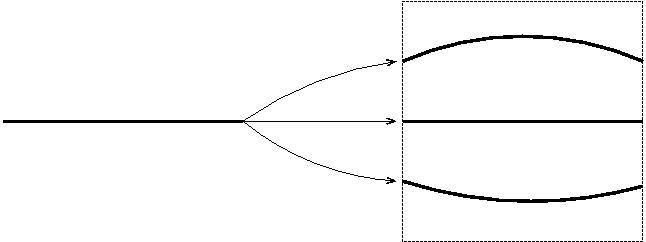
Figure 1: Spacetime, $M$, is foliated by a one-parameter family of embeddings $\mathcal{E}_{t}$ of the 3-manifold $\Sigma$ into $M$. Here $t$ is a formal label without direct physical significance. $\Sigma_{t}$ is the image in $M$ of $\Sigma$ under $\mathcal{E}_{t}$. Each such $\Sigma_{t}$ is an instant.

In particular, these conditions ensure that the spacetime can be thought of as the history of space. In a loose mathematical sense this means that spacetime is a staking of spaces, each one being an instant. More precisely, spacetime is foliated by a one-parameter family of embeddings of space into spacetime. This is schematically represented in Figure 1. For that to make mathematical sense we must be sure that a single space, $\Sigma$, suffices to foliate spacetime. Its geometry may change from leaf to leaf, but not its essential properties as differentiable manifold, for otherwise we could not speak of its evolution. In particular this means that its topological properties are preserved during evolution, like its connectedness and its higher topological invariants; see Figure 2.

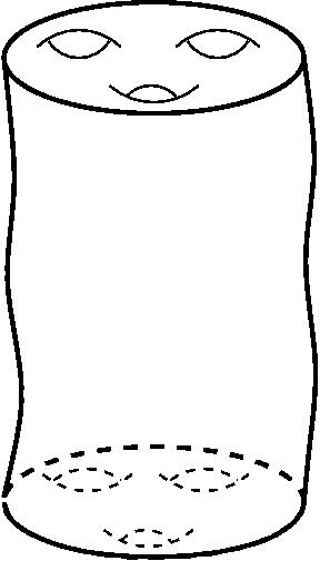
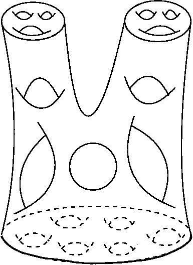
Figure 2: Schematic rendering of spacetimes. The one on the left may be viewed as time evolution of space. Time runs upwards and space corresponds to the horizontal sections, here depicted by a 3-holed surface. In the spacetime on the right an initial connected space at the bottom, represented by a single 6-holed surface, evolves into two 3-holed pieces. This spacetime cannot be viewed as time evolution of a single space and shall be excluded from the discussion.

One of the fundamental difficulties with the notion of spacetime as history of space is its inherent redundancy: There are many ways to describe one and the same spacetime as the evolution of space. This is explained in Figure 3. This means that if we cast Einstein’s equations into the form of evolution equations for “space”, we cannot expect unique solutions, contrary to what is usually required for well posed initial-value problems. The point here is that the non-uniqueness is not arbitrary. It is precisely of the amount that accounts for the different ways to move space through a fixed spacetime, no more and no less. This is closely related to the infamous “Hole Argument” [15].

Figure 3: There is a large ambiguity in moving from an initial space-slice $\Sigma_{t}$ “forward in time”. For $q\in\Sigma$ the image points $p=\mathcal{E}_{t}(q)$ and $p^{\prime}=\mathcal{E}_{t+dt}(q)$ are connected by the vector $\partial/\partial t|_{p}$ whose components tangential and normal to $\Sigma_{t}$ are $\beta$ (three functions) and $\alpha n$ (one function) respectively. Hence there is a four-function worth of ambiguity to move $\Sigma_{t}$ in a given ambient spacetime.

That relaxation of the uniqueness requirement is familiar from so-called “gauge-theories” and does not imply any renunciation from determinism of fundamental laws, at least as long as the degree of arbitrariness in the analytical expression of the evolution is under complete mathematical control. Physical configurations are then taken to be the equivalence classes under the relation that identifies any two apparently different evolutions that give rise to the same spacetimes (more precisely: diffeomorphism-class of spacetimes).

The Chronos principle

Modulo the difficulties just mentioned, we may ask whether we can extract a notion of time merely from the information of instants. An instant here is a spatial configuration, that is a pair $(\Sigma,h)$, where $\Sigma$ is a 3-dimensional manifold and $h$ is a Riemannian (i.e. positive definite) metric. One obvious question concerning Einstein’s equations is this: given two instants $(\Sigma_{1},h_{1})$ and $(\Sigma_{2},h_{2})$, can we associate a measure of time by which they are apart if we assume that both 3-geometries occur in a spacetime that satisfies Einstein’s equations. This is known as the “sandwich conjecture” in General Relativity and known to fail in many known examples which are, however, of special symmetry that renders the problem singular. For example, it is obvious that specifying any two flat 3-slices in Minkowski space does not give us any information on their separation. Similarly, it has been shown that in the spherically symmetric case a similar underdetermination prevails [16]. On the other hand, it has been an old hope that a suitable analog of Jacobi’s principle, and in particular formula (8), is also valid in General relativity. This has been first proposed in the classic and well known paper [1] of 1962. An apparently less well known contribution appeared 12 years later, in which the following “Chronos Principle” in General Relativity was proposed, according to which time is a measure for the distance of instantaneous configurations (instants) [6]. Moreover, it was asked in [6] whether such measures existed such that one would not have to know the entire spatial configuration in order to determine the time span.

“This postulate contains the statement that it is not necessary to look at the change in configuration of the entire universe to measure time. It is sufficient to measure the change in configuration of only a localized region of the universe, and one is assured that the local time thus obtained will be equal to that of any other region, and indeed equal to the global time.” ([6], p. 76)

It is this localisation property that renders this reading of time from instants physically viable. Let us therefore see how it can be satisfied. The answer, quite surprisingly, leads more or less directly to General Relativity. We shall give the argument in a slightly simplified form.

As already stated, Einstein’s equations can be cast into evolutionary form. In that form one may identify a kinetic-energy metric, just like in point mechanics. It reads:

$$ds^{2}=\int_{\Sigma}d^{3}x\ G^{ab\,nm}[h(x)]dh_{ab}(x)dh_{nm}(x)$$ (11)

where $G^{ab\,nm}[h(x)]$ is a certain expression that depends on the metric tensor $h$ of space but not on its derivatives (ultralocal dependence). It is sometimes called the Wheeler-DeWitt metric. The measure of time will be obtained by a rescaling of the kinetic-energy metric, just like in (8). Hence one writes

$$d\tau^{2}=\frac{ds^{2}}{\int_{\Sigma}d^{3}x\ R(x)}\,.$$ (12)

Here $R$ must be a scalar function of the spatial metric $h$. The simplest non-constant such function is the scalar curvature, which depends on $h$ and its derivatives up to order 2. The condition that the measure of time be compatible with arbitrarily fine localisation $\Sigma\rightarrow U\subset\Sigma$ leads requires the integrands in the numerator and denominator of (12) to be proportional. Without loss of generality we can take this constant of proportionality (which cannot be zero) to be $1$ (this just fixes the overall scale of physical time) and obtain

$$G^{ab\,nm}[h(x)]\frac{dh_{ab}(x)}{d\tau}\frac{dh_{nm}(x)}{d\tau}-R[h](x)=0\,.$$ (13)

This is a well known formula (the so-called Hamiltonian constraint) in General Relativity. Hence Relativity just satisfies the localisation property with the simplest conceivable local rescaling function $R$. Finally, physical time is now given in terms of 3-dimensional geometric quantities by a Jacobi-like formula, which is just the analog of (8) in the case $E=0$:

$$\Delta\tau(\mathbf{g}_{i},\mathbf{g}_{f})=\int_{\mathbf{g}_{i}}^{\mathbf{g}_{f}}\sqrt{\frac{G\bigl{(}d\mathbf{g}/d\lambda,d\mathbf{g}/d\lambda\bigr{)}}{-R\bigl{[}\mathbf{g}(\lambda)\bigr{]}}}\ d\lambda$$ (14)

4 Conclusions and open issues

Following [2] we tried to argue that the notion of “time from instances” in inherent in classical point mechanics as well as General Relativity. We also saw that in General Relativity that notion of time is not as hopelessly global as one might have feared. In fact, one can argue that General Relativity just realises the simplest localisable notion of that sort of time.

But there are also points that remain open (to me):

1. Solutions to dynamical equations of motion in the form of (generalised) geodesic principles are subsets of (dynamically realised) configurations in the space of (kinematically possible) ones. These subsets are delivered to us in the form of unparametrised curves. So, even though the parameter does not matter, the structure of a one-dimensional sub-continuum remains. In particular one (or two) preferred orderings are selected. What is the significance of that? What makes us experience this solution configurations according to this order?

2. Can we, on the space of 3-geometries, characterise a function that structures it according to some definition of geometric entropy? How would its gradient flow be related to the dynamics of General Relativity?

3. Suppose the spacetime we live in did not allow for any symmetries and were sufficiently generic, so as to not allow for two different isometric embeddings of any of its possible 3-geometries. (Such spacetimes exist and are, intuitively speaking, the generic case, though their degree of generality or naturalness is not easy to characterise mathematically.) This means that each instant would have its unique place in spacetime. Would this count as a perfect representation of the “Now” in a physical theory (here General Relativity), or could/should we ask for more?

Finally I wish to comment on the transition of point mechanics to field theory. In point mechanics, the requirement to only employ purely relational quantities is met by eliminating all explicit reference to absolute space and time. This has been gradually achieved in the papers of Reissner, Schrödinger, and Barbour & Bertotti. But what is the precise analog of that requirement in field theory? A standard answer to this is that the theory should be background independent. The intended meaning of that phrase is that the theory should not employ structures which are not dynamically active. Closer inspection shows that it is quite hard to translate this intended meaning into a clear mathematical condition [9]. The problem is that whatever the mathematical formulation is, it seems quite easy to turn it into an equivalent one by some formal rewriting that renders it (formally) background independent. It is often taken for granted that the requirement of diffeomorphism invariance (also known as “general covariance”) is sufficient, because that would deprive spacetime points of their independent individuality. This is true to some extend, but it seems not to go as far as one might have hoped for. Modern (quantum-)field theory does not get rid of space and time.

Markus Fierz was deeply concerned about the problematic relation between spacetime and fields. In a remarkable letter of October 9-10th 1951 to Wolfgang Pauli he wrote ([12], Vol. IV, Part I, Doc. 1287, p. 379)

“There exist [in classical physics–DG] solutions [to field equations–DG] with empty domains, that is, emptied from all fields. Hence one needs a theory of space which is independent of what fills space. There is the geometry of space and the laws of things in space. […]

Space is still absolute in Relativity Theory insofar as one may characterise it without referring to its ‘content’, and because it may even exist without any content. […]

In a [hypothetical–DG] full Theory of Quantum Fields, in which the act of observation and the possibility to localise are described correctly, it should not be necessary to introduce space separately. Opposite to what Einstein hoped, the laws of space should follow from the laws of Nature (not the laws of Nature from geometry). But this can only be hoped for if there is no such thing as empty space, that is, if you cannot clear [ausräumen] space. Fields are not in space, they span space. Space is not a geometric idea [Gedankending], it is a certain aspect of the world.”

In this sense, space in Relativity Theory is absolute and this is why Einstein suggested to call it aether. In a proper field theory the theory of localisation should deliver a theory of space. Space should somehow be ‘created’ by test bodies and hence be a function of the observer in a much deeper sense than in Relativity Theory.”

Pauli replied on October 13 in a way that would also be typical for many modern relativists ([12], Vol. IV, Part I, Doc. 1289, pp. 385-386):

“Your wording does not do justice to Relativity Theory, which is just an attempt to connect geometry and laws of nature concerning things [Dinge] in the spacetime world. […] All people happily proclaim just the opposite to what you said in your letter: namely ‘from now on only the connection of spacetime and things is absolute. […]

I am quite indignant about this part of your letter, since it shows to me that the, compared to me, slightly younger generation of physicists (not to speak of the still younger ones!) have completely repressed [verdrängen] General Relativity - and because I know how important Einstein considered this point to be. […]

After this urgent correction (diagnosis: ‘repression’ [Verdrängung]!) one can ask whether the dependence of space (i.e. spacetime) from the things [Dingen] according to General Relativity is sufficient. To pose the question already means to negate it. […]

I agree that the impossibility to accommodate Einstein’s postulate (i.e. Mach’s original point of view) within General Relativity is a deep and significant sign for the inadequacy of classical field physics.”

So we see that after his usual grumble Pauli finally agrees at least on the existence of a fundamental difficulty, which was, after all, well addressed by Fierz’ original complaint. Even today all candidate theories of quantum gravity make use of non-dynamical structures that represent some sort of space or spacetime (of various dimensions). Hence I believe Fierz’ complaint is as as relevant today as it was 60 years ago.

Everyone knows the opening words of Hermann Minkowski’s (1864-1909) famous address “Raum und Zeit”, delivered in Cologne on September 21st 1908 [13]:

“Gentlemen! The views of space and time which I wish to lay before you have sprung from the soil of experimental physics. Therein lies their strength. They are radical. Henceforth space by itself, and time by itself, are doomed to fade away into mere shadows, and only a kind of union of the two will preserve an independent reality.”

But it seems not to be so well known that Minkowski felt the enormous abstraction and possible physical over-idealisation of the concept of spacetime as such, as he clearly indicated in his introduction, before going into the description of what we now call “Minkowski space” (space meaning spacetime). He wanted his readers to understand the points of spacetime as individuated entities:

“In order to not leave a yawning void [gähnende Leere], we wish to imagine that at every place and at every time something perceivable exists. In order to avoid saying ‘matter’ or ‘electricity’ for that something, I will use the word ‘substance’ for it. We focus attention on the substantive [substantiellen] world point at $x,y,z,t$ and imagine to be capable to recognise this substantive point at any other time”.

That substantivalist’s view of Minkowski spacetime is still inherent in its mathematical representation in modern field theory. One sign of this is the interpretation of its automorphism group (the Poincaré group) as proper physical symmetries rather than gauge transformations. Recall that a proper physical symmetry transforms solutions to dynamical equations into solutions, but the transformed solution is considered physically different (distinguishable) from the original one. In contrast, gauge transformations just connect redundant descriptions of the same physical situation.

Individuating spacetime points is natural if we think of spacetime to be a geometrically structured set. A set, by Cantor’s definition, consists first of all of a set which may then carry certain geometric structures of various complexities. But recall what according to Cantor’s definition it already takes to be a set [5]:

“By a set we understand any gathering together $M$ of determined well-distinguished objects $m$ of our intuition or of our thinking (which are called elements of $M$) into a whole.”

Minkowski’s “substance” may serve to distinguish events. But is that substance not eventually just another physical system obeying its own dynamical laws? If so, what kind of “dynamical law” can that be if there is no non-dynamical substance left with respect to which we can define change. Surprisingly – or perhaps not – this is just the same difficulty that stood at the very beginning of modern theories of dynamics. In “de gravitatione”, written well before the Principia, presumably between 1664 and 1673 (the dating is still controversial), Newton said [14]:

“It is accordingly necessary that the determination of places and thus of local motions is represented in some unmoved being of which sort space or extension alone is that which is seen as distinct from bodies. […]

About extension, then, it is probably expected that it is being defined either as substance or accidents or nothing at all. But by no means nothing, surely, therefore it has some mode of existence proper to itself, by of which it fits neither to substance nor to accident.”

“Das noch Ältere ist immer das Neue”
Wolfgang Pauli

Acknowledgements

I sincerely thank Albrecht von Müller and Thomas Filk for several invitations to workshops of the Parmenides Foundation, during which I was given the opportunity to present and discuss the material contained in this contribution.

References

- [1] Ralph F. Baierlein, David H. Sharp, and John A. Wheeler. Three-dimensional geometry as carrier of information about time. Physical Review, 126(5):1864–1865, 1962.
- [2] Julian B. Barbour. The timelessness of quantum gravity: I. the evidence from the classical theory. Classical and Quantum Gravity, 11(12):2853–2873, 1994.
- [3] Julian B. Barbour and Bruno Bertotti. Mach’s principle and the structure of dynamical theories. Proceeding of the Royal Society A, 382(1783):295–306, 1982.
- [4] Julian B. Barbour and Herbert Pfister. Mach’s Principle: From Newton’s Bucket to Quantum Gravity, volume 6 of Einstein Studies. Birkhäuser, Basel, 1995.
- [5] Georg Cantor. Beiträge zur Begründung der transfiniten Mengenlehre. (Erster Artikel). Mathematische Annalen, 46:481–512, 1895.
- [6] Demetrios Christodoulou. The chronos principle. Il Nuovo Cimento, 26 B(1):67–93, 1975.
- [7] Gerald M. Clemence. On the system of astronomical constants. The Astronomical Journal, 53(6):169–179, 1948.
- [8] Domenico Giulini. Das Problem der Trägheit. Philosophia Naturalis, 39(2):843–374, 2002.
- [9] Domenico Giulini. Some remarks on the notions of general covariance and background independence. In Erhard Seiler and Ion-Olimpiu Stamatescu, editors, Approaches to Fundamental Physics, volume 721 of Lecture Notes in Physics, pages 105–120. Springer, Berlin, 2007. Online available at arxiv.org/pdf/gr-qc/0603087.
- [10] Ludwig Lange. Über das Beharrungsgesetz. Berichte über die Verhandlungen der königlich sächsischen Gesellschaft der Wissenschaften zu Leipzig; mathematisch-physikalische Classe, 37:333–351, 1885.
- [11] Ned Markosian. Time. In Edward N. Zalta, editor, The Stanford Encyclopedia of Philosophy. Winter 2010 edition, 2010.
- [12] Karl von Meyenn, editor. Wolfgang Pauli: Scientific Correspondence with Bohr, Einstein, Heisenberg, a.O., Vol. I-IV, volume 2,6,11,14,15,17,18 of Sources in the History of Mathematics and Physical Sciences. Springer Verlag, Heidelberg and New York, 1979-2005.
- [13] Hermann Minkowski. Raum und Zeit. Verlag B.G. Teubner, Leipzig and Berlin, 1909. Address delivered on 21st of September 1908 to the 80th assembly of german scientists and physicians at Cologne.
- [14] Isaac Newton. Über die Gravitation. Vittorio Klostermann, Frankfurt a.M., 1988.
- [15] John D. Norton. The hole argument. In Edward N. Zalta, editor, The Stanford Encyclopedia of Philosophy. Fall 2011 edition, 2011.
- [16] Niall Ó Murchadha and Krzysztof Roszkowski. Embedding spherical spacelike slices in a Schwarzschild solution. Classical and Quantum Gravity, 23(2):539–547, 2006.
- [17] Hans Reissner. über die Relativität der Beschleunigung in der Mechanik. Physikalische Zeitschrift, 15:371–375, 1914.
- [18] Erwin Schrödinger. Die Erfüllbarkeit der Relativitätsforderung in der klassischen Mechanik. Annalen der Physik (Leipzig), 77:325–336, 1925.
- [19] Peter Guthrie Tait. Note on reference frames. Proceedings of the Royal Society of Edinburgh, XII:743–745, Session 1883-84.
- [20] James Thomson. On the law of inertia; the principle of chronometry; and the principle of absolute clinural rest, and of absolute rotation. Proceedings of the Royal Society of Edinburgh, XII:568–578, Session 1883-84.