Algorithms and Stability Analysis for Content Distribution over Multiple Multicast Trees

Abstract

The paper investigates theoretical issues in applying the universal swarming technique to efficient content distribution. In a swarming session, a file is distributed to all the receivers by having all the nodes in the session exchange file chunks. By universal swarming, not only all the nodes in the session, but also some nodes outside the session may participate in the chunk exchange to improve the distribution performance. We present a universal swarming model where the chunks are distributed along different Steiner trees rooted at the source and covering all the receivers. We assume chunks arrive dynamically at the sources and focus on finding stable universal swarming algorithms. To achieve the throughput region, universal swarming usually involves a tree-selection subproblem of finding a min-cost Steiner tree, which is NP-hard. We propose a universal swarming scheme that employs an approximate tree-selection algorithm. We show that it achieves network stability for a reduced throughput region, where the reduction ratio is no more than the approximation ratio of the tree-selection algorithm. We propose a second universal swarming scheme that employs a randomized tree-selection algorithm. It achieves the throughput region, but with a weaker stability result. The proposed schemes and their variants are expected to be useful for infrastructure-based content distribution networks with massive content and relatively stable network environment.

I Introduction

The Internet is being used to transfer content on a more and more massive scale. A recent innovation for efficient content distribution is a technique known as swarming. In a swarming session, the file to be distributed is broken into many chunks at the original source, which are then spread out across the receivers. Subsequently, the receivers exchange the chunks with each other to speed up the distribution process. Many different ways of swarming have been proposed, such as FastReplica [LeeV07], Bullet [Bullet'], Chunkcast [Chunkcast], BitTorrent [BitTorrent], and CoBlitz [CoBlitz].

The swarming technique was originally introduced by the end-user communities for peer-to-peer (P2P) file sharing. The subject of this paper is how to apply swarming to infrastructure-based content distribution, where files are to be distributed among content servers in a content delivery network. The content servers are usually connected with leased high-speed links and, as a result, the bandwidth bottleneck may no longer be at the access links. It has been shown that content delivery traffic has made capacity shortage in the backbone networks a genuine possibility [CFE06]. The size of such a content distribution network is usually small, consisting of up to hundreds of network nodes and up to thousands of servers. Unlike the dynamic end-user file-sharing situations, infrastructure networks and content servers are usually centrally managed, generally well-behaved and relatively static (however, the traffic can still be dynamic). In this setting, it is beneficial to view swarming as distribution over multiple multicast trees, each spanning the content servers. This view allows us to pose the question of how to optimally distribute the content (see [ZCX08]). Furthermore, it is often easier to first develop sophisticated algorithms under this tree-based view, and then, adapt them to practical situations where the tree-based view is only partially adequate. Hence, in this paper, swarming is synonymous to distribution over multiple multicast trees.

This paper concerns a class of improved swarming techniques, known as universal swarming. We associate with each file to be distributed a session, which consists of the source of a file and the receivers who are interested in downloading the file. In traditional swarming, chunk exchange is restricted to the nodes of the session. However, in universal swarming, multiple sessions are combined into a single “super session” on a shared overlay network. Universal swarming takes advantages of the heterogenous resource capacities of different sessions, such as the source upload bandwidth, receiver download bandwidth, or aggregate upload bandwidth, and allows the sessions to share each other’s resources. The result is that the distribution efficiency of the resource-poor sessions can improve greatly with negligible impact on the resource-rich sessions (see [ZCX09-1a]).

In universal swarming, if we focus on a particular file, not only the source and all the receivers participate in the chunk exchange process, some other nodes who are not interested in the file may also participate. We call the latter out-of-session nodes. To illustrate the essence of universal swarming, as well as the main issues, consider the toy example in Fig. 1. The numbers associated with the links are their capacities. Let us consider a particular file for which the source is node 1 and the receivers are nodes 2 and 3. Node 4 is out of the session. Let us focus on a fixed chunk and consider how it can be distributed to the receivers. With some thoughts, it can be seen that the chunk propagates on a tree rooted at the source and covering both receivers. All possible distribution trees are shown in Fig. 2. We notice that a distribution tree may or may not include the out-of-session node, 4. Thus, a distribution tree in general is a Steiner tree rooted at the source covering all the receivers, where the out-of-session nodes (e.g., node 4) are the Steiner nodes.

With this model of multi-tree multicast, one of the main questions is how to assign the chunks to different distribution trees so as to optimize certain performance objective, such as maximizing the sum of the utility functions of the sessions, or minimizing the distribution time of the slowest session. This is a rate allocation problem on the multicast trees. One such question was addressed in [ZCX08] in the context of non-universal swarming, where each session’s multicast trees are spanning trees instead of Steiner trees. For universal swarming, the question was addressed in [ZCX09-1a].

This paper addresses the stability problem. The main question is: Given a set of data rates from the sources (which are possibly the solutions to the aforementioned rate allocation problem), how do we get a universal swarming algorithm so that the network queues will be stable? For the example in Fig. 1, a source rate of 2 is the largest distribution rate that can be supported by the network if everything is deterministic. To achieve stability under random arrivals, it usually requires that the data arrival rate is strictly less than 2 (for a justification, consider a single-queue system). Hence, when the file chunks arrive at (or generated by) the source node 1 at a mean rate $2-2\epsilon$, where $0<\epsilon<1$, we can place chunks on the first and the second tree in Fig. 2 at a mean rate $1-\epsilon$ each. For this example, the solution actually stabilizes the network. But, this conclusion requires technical conditions and is not generally true for more complicated situations.

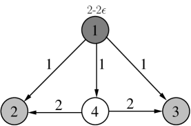
Figure 1: Node 1 sends the file to nodes 2 and 3.

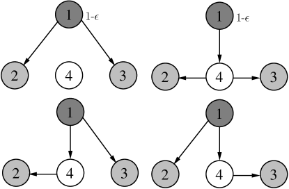
Figure 2: All possible distribution trees for the example in Fig. 1.

In this paper, we develop a universal swarming scheme that employs an approximation algorithm to the tree selection (a.k.a. scheduling) problem, which achieves a rate region equal to the throughput region reduced by a constant factor $\gamma$, $\gamma\geq 1$. We show that $\gamma$ is no more than the approximation ratio of the tree scheduling algorithm. The scheme requires network signaling and source traffic regulation. We propose a second universal swarming scheme that utilizes a randomized tree selection algorithm, which achieves the entire throughput region, but with a weaker stability property.

The difference between our problem and the wireless scheduling problems is substantial. Most previous papers that consider multi-hop traffic are either in the unicast setting or in a multicast setting with a few fixed multicast trees per multicast session. We must consider multi-hop, multicast communications, and, to have the largest possible throughput region, we allow each multicast session to use any multicast trees for the session. The combination of these three features makes our problem both unique and very hard. One of the main challenges is that there is no obvious way to specify the packet forwarding behavior without per-tree queueing (i.e., having a separate queue for each multicast tree) whereas, on the other hand, per-tree queueing is impractical due to the exceedingly large number of trees. Our solution to resolve this difficulty, on the algorithm side, is to use the techniques of signaling and virtual queueing. The techniques allow us to have very small numbers of queues and at the same time show stability guarantee.

Having avoided per-tree queueing, however, the performance analysis is still difficult. In particular, there is no easy way to prove the stability of the real queues. Our analytical approach is to first prove the stability of the virtual queues. The proofs in this step are relatively conventional, using the techniques of Lyapunov drift analysis. The second step is to make connections between the virtual queues and the real queues, and use the stability results for the virtual queues to prove that the real queues are also stable.

The tree selection subproblem is inherent to the problem formulated in the paper and it remains difficult. As a remedy, our algorithms can work with low-cost trees as opposed to the min-cost trees; finding low-cost trees can be much easier. The stability results are applicable to classes of algorithms by allowing different tree selection sub-algorithms. Hence, the research for finding simpler, more practical algorithms can continue.

The rest of the paper is organized as follows. The models and the problem description are given in Section II. The first universal swarming scheme and the analysis are presented in Section III. The second universal swarming scheme and the analysis are presented in Section LABEL:sec:without_regulator. In Section LABEL:sec:related, we discuss additional related work. The conclusion is in Section LABEL:sec:conclusion.

II Problem Description

We consider a time-slotted system where each time slot has a duration of one time unit. Let the network be represented by a directed graph $G=(V,E)$, where $V$ is the set of nodes and $E$ is the set of links. For each link $e\in E$, let $c_{e}$ denote its capacity (e.g., in the number of file chunks it can transmit per time slot), where $c_{e}>0$. We assume that each session, which distributes a distinct file, has one source, and hence, there is a one-to-one mapping between a session and a source. Let $S$ denote the set of sources (sessions). For each $s\in S$, let $V_{s}\subseteq V$ be the set of receivers associated with the source (session) $s$.

For each source $s\in S$, suppose constant-sized data packets (i.e., file chunks) arrive at the source according to a random process, which will be distributed over the network to all the receivers, $V_{s}$. The motivation for using a source model with dynamic arrivals is to account for the end-system bottleneck and timing variations in reading and transmitting locally stored data. In some cases, the content may not be a static file or stored locally. The model is general enough to cover realtime content, streaming video with time-varying rate, or non-locally stored static data. Even if the entire file is static and stored at the source, this source model can still be useful. For instance, the data packets can be injected into the source node at a constant rate, which corresponds to a deterministic arrival process with a constant arrival rate. Let $A_{s}(k)$ be the number of packet arrivals on time slot $k$. Let us make the following assumption on the arrival processes $\{A(k)\}$ throughout the paper, unless mentioned otherwise. Additional assumptions may be added as needed.

AS 1.

For each source $s\in S$, $E[A_{s}(k)|x(k)]=\lambda_{s}$, and $E[(A_{s}(k))^{2}|x(k)]<K_{1}$ for some $0<K_{1}<\infty$, for all time $k$, where $x(k)$ represents the system state at time $k$.

The following are some remarks about Assumption AS 1.

• The system state, $x(k)$, will depend on the specific settings of the two algorithms considered in this paper and will become clear later. It usually includes all the queue sizes at time $k$, and possibly some additional auxiliary variables. If the arrival process is independent of the past for each source $s$, assumption AS 1 can be stated without conditioning on $x(k)$. However, some non-IID arrival processes can lead to dependence between the current arrivals and the current queue sizes, in which case the statement with conditioning is more general than one without conditioning.

• If the arrival process is independent of the past for each source $s$, assumption AS 1 can be stated without the conditioning.

• $(\lambda_{s})_{s\in S}$ could be the solution of a rate allocation problem (see the discussion about the rate allocation and stability problems in Section I).

In this paper, we will present stable universal swarming algorithms to distribute the packets to all the receivers. For each $s\in S$, the packets will be transmitted along various multicast distribution trees rooted at $s$ to the receivers in $V_{s}$. A multicast tree in the multicast case corresponds to a path between a sender and a receiver in the unicast case. Hence, using multiple multicast trees for a multicast session is analogous to data delivery using multiple paths between a sender and a receiver in the unicast case.

We will take Neely’s definition of stability ([Neely-IT06]; [Neely03], chapter 2) unless mentioned otherwise. For a single-queue process $\{q(k)\}$, let us define the overflow function:

$$g(M)=\limsup_{K\rightarrow\infty}\frac{1}{K}\sum_{k=1}^{K}P\{q(k)>M\}.$$ (1)

Roughly speaking, the overflow function $g(M)$ in (1) defines the long-time average fraction of time when the queue size $q(k)$ is more than a chosen threshold $M$. In the stationary and ergodic case, it coincides with the stationary (and limiting) probability that the queue size exceeds $M$.

Definition 1.

The single-queue process $\{q(k)\}$ is stable if $g(M)\rightarrow 0$ as $M\rightarrow\infty$. A network of queues is stable if every queue is stable.

With this definition of network stability, a sufficient condition for network stability is: Some Lyapunov function of the queues has a negative drift when any of the queues becomes large enough [Neely-IT06] [Neely03] [NML08] [Neely2010]. If with additional assumptions, the network queues form an ergodic Markov chain, the same drift condition implies the chain is positive recurrent, or equivalently, has a stationary distribution.

II-A Throughput Region

For each source $s\in S$, let the set of candidate distribution trees be denoted by $T_{s}$. Throughout this paper, $T_{s}$ contains all possible distribution trees rooted at the source $s$ unless specified otherwise. Let $T=\cup_{s\in S}T_{s}$. The trees can be enumerated in an arbitrary order as $t_{1},t_{2},\cdots,t_{|T|}$, where $|\cdot|$ denote the cardinality of a set. Although $|T|$ is finite, it might be very large.

The throughput region is defined as

$$\Lambda=\{\lambda\geq 0:\exists\alpha\geq 0\mbox{ such that }\sum_{t\in T_{s}}\alpha_{t}=1,\forall s\in S\mbox{ and }\sum_{s\in S}\ \ \sum_{\{t\in T_{s}|e\in t\}}\alpha_{t}\lambda_{s}\leq c_{e},\forall e\in E\}.$$ (2)

Here, $\alpha$ represents how the traffic from the sources is split among the distribution trees. The definition of $\Lambda$ says that a source rate vector $\lambda$ is in $\Lambda$ if there exists a set of tree rates for each multicast session such that the resulting total link data rate is no more than the link capacity for any link. Obviously, $\Lambda$ contains the stability region, i.e., all $\lambda$ that can be stabilized by some algorithms. This is so because, for any non-negative mean rate vector $\lambda\not\in\Lambda$, no matter how the traffic is split among the distribution trees, there exists a link $e$ such that the total arrival rate to $e$ is strictly greater than its service rate. Furthermore, this definition of the throughput region allows the bandwidth bottleneck to be anywhere in the network, at the access links or at the core.

We also define a $\gamma$-reduced throughput region as $\frac{1}{\gamma}\Lambda$, where $\gamma\geq 1$. By saying that the arrival rate vector $\lambda$ is strictly inside the region $\frac{1}{\gamma}\Lambda$, we mean that there exist some $\epsilon_{0}>0$ and a vector $\alpha\geq 0$ such that $\sum_{t\in T_{s}}\alpha_{t}=1,\forall s\in S$ and $\sum_{s\in S}\sum_{\{t\in T_{s}|e\in t\}}\alpha_{t}\lambda_{s}\leq\frac{1}{\gamma}c_{e}-\epsilon_{0},\forall e\in E$. This is equivalent to

$$c_{e}\geq\gamma(\epsilon_{0}+\sum_{s\in S}\sum_{\{t\in T_{s}|e\in t\}}\alpha_{t}\lambda_{s}),\ \ \forall e\in E.$$ (3)

Note that the region of rate vectors that are strictly inside the region $\frac{1}{\gamma}\Lambda$ contains the interior of $\frac{1}{\gamma}\Lambda$. In Section III, we will show that the interior of $\Lambda$ is stabilizable. That is, for any rate vector $\lambda$ strictly inside the region $\Lambda$, there exists a scheduling algorithm such that the queues in the network are stable under the algorithm.

II-B The Class of Algorithms: Time Sharing of Trees

Each source has at least two possible approaches to use the multicast trees. In one approach, the traffic from each source $s$ may be split according to some weights $(\alpha_{t})_{t\in T_{s}}$ and transmitted simultaneously over the trees on every time slot. Alternatively, the distribution can be done by time-sharing of the trees. The algorithms in this paper follow the time-sharing approach. On each time slot $k$, the source $s$ selects one distribution tree from the set $T_{s}$, denoted by $t_{s}(k)$, according to some tree-scheduling (tree-selection) scheme, and transmits packets only over this tree on time slot $k$. The time-sharing approach can emulate the first approach in the sense that, when done properly, the fraction of time each distribution tree is used over a long period of time can approximate any weight vector $(\alpha_{t})_{t\in T_{s}}$.

In addition to selecting the distribution tree $t_{s}(k)$ at each time slot, an algorithm also needs to decide how many packets are released to the tree. We will present two algorithms in the following sections. The key question is what portion of the rate region is stabilizable by each algorithm.

III Signaling, Source Traffic Regulation and $\gamma$-approximation Min-Cost Tree Scheduling

III-A Signaling Approach

Stability analysis of a multi-hop network is often difficult because the packets travel through the network hop-by-hop, instead of being imposed directly to all links that they will traverse. As a result, the arrival process to each internal link can be difficult to describe. The frequently-used technique of network signaling can be helpful. In our case, on each time slot $k$, each source $s$ sends one signaling packet to each node on the currently selected tree $t_{s}(k)$. A signaling packet is one of the two types of control packets in the paper. It has two main functions. The first is to set up the multicast tree $t_{s}(k)$. A signaling packet contains a list of link IDs, which describe to the receiving node which of its outgoing links are part of the multicast tree. The second function is to inform the receiving node the intended source transmission rate on time slot $k$, i.e., the number of packets to be transmitted on time slot $k$. To make the proofs for the main results easier, we make the following assumptions about all control packets, including the forward signaling packets and the feedback packets: The control packets are never lost and they arrive at their intended destinations within the same time slot on which they are first transmitted. Note that these assumptions are not crucial for either the theory or practice. We do not make any assumptions on the data packets.

We will see that the rate information contained in a signaling packet is a very tight upper bound on the number of real packets released by the source on that time slot. To mark the the slight discrepancy, we use the term virtual packets and call the rate contained in the signaling packet the rate of virtual packets or the virtual source rate. Consider a particular time slot $k$ and a particular internal link $e$ on the selected distribution tree. The real packets issued by the source on time slot $k$ will in general be delayed or buffered at upstream hops and will not arrive at link $e$ until later. However, via signaling, link $e$ knows how many virtual packets are injected by the source and arrive at link $e$ on time slot $k$. The cumulative number of arrived real packets at link $e$ must be no more than the cumulative number of arrived virtual packets (via signaling packets).

One question is how many real packets are to be released to the network on a time slot. One possibility is that each source $s$ releases all the packets that arrive during time slot $k$, i.e., $A_{s}(k)$. However, the uncontrolled randomness of $A_{s}(k)$ causes difficulty in the stability analysis, as we will see later. In our algorithm, each source $s$ sets the number of real packets to be released at the constant value $\lambda_{s}+\epsilon_{1}$ on every time slot $k$, if that number of real packets is available. Every signaling packet from source $s$ contains the constant virtual packet rate $\lambda_{s}+\epsilon_{1}$. Here, $\epsilon_{1}$ is a sufficiently small constant such that $0<|S|\epsilon_{1}<\epsilon_{0}$. This guarantees the stability of the source regulators, as we will see.

In the algorithm, each link $e$ updates a virtual queue, denoted by $q_{e}(k)$.

$$q_{e}(k+1)=[q_{e}(k)+\sum_{s\in S:e\in t_{s}(k)}(\lambda_{s}+\epsilon_{1})-c_{e}]_{+}.$$ (4)

$[\cdot]_{+}$ is the projection operation onto the non-negative domain. Note that the second term on the right hand side of (4) is the aggregate virtual data arrival rate from all the trees containing link $e$, which means the link capacities are shared by different trees. Tree scheduling is based on the virtual queues instead of the real queues.

III-B Source Traffic Regulation

A regulator is placed at each source $s$ to ensure that on each time slot, source $s$ transmits no more than $\lambda_{s}+\epsilon_{1}$ real packets. A regulator is a traffic shaping device. All the packets arriving at source $s$ first enter a regulator queue. They will be released to the network later in a controlled fashion. On each time slot $k$, let $D_{s}(k)$ denote the number of real packets released from the regulator to the distribution tree $t_{s}(k)$, and let $p_{s}(k)$ be the regulator queue size at source $s$. The evolution of the regulator queue is given by

$$p_{s}(k+1)=p_{s}(k)+A_{s}(k)-D_{s}(k),$$ (5)

where

$$D_{s}(k)=\left\{\begin{array}[]{ll}\lambda_{s}+\epsilon_{1}&\mbox{if $p_{s}(k)\geq\lambda_{s}+\epsilon_{1}$};\\ p_{s}(k)&\mbox{otherwise}.\end{array}\right.$$ (6)

Expressions (6) ensures that at most $\lambda_{s}+\epsilon_{1}$ real packets are released on each time slot. Since this departure rate is higher than the mean packet arrival rate, stability of the regulator is guaranteed. We will provide more details in the stability analysis. Note that the traffic regulators are required only at the sources and they can be implemented at the end-systems, i.e., the content servers.

III-C $\gamma$-Approximation Min-Cost Tree Scheduling

We can interpret the virtual queue size $q_{e}$ as the cost of link $e$. Then, the cost of a tree $t$ is $\sum_{e\in t}q_{e}$. We propose the $\gamma$-approximation min-cost tree scheduling scheme: On each time slot $k$ and for each source $s$, the selected tree $t_{s}(k)$ satisfies

$$\sum_{e\in t_{s}(k)}q_{e}(k)\leq\gamma\min_{t\in T_{s}}\sum_{e\in t}q_{e}(k),$$ (7)

where $\gamma\geq 1$. If there are multiple trees satisfying (7), the tie is broken arbitrarily.

The rationale for this tree-scheduling scheme is straightforward. When $\gamma=1$, the tree-scheduling scheme solves the min-cost Steiner tree problem, which is NP-hard. But, the min-cost Steiner tree problem has approximation solutions, which we can use. In [ChaChe99], a family of approximation algorithms for the directed Steiner tree problem is proposed, which achieves an $O(\log^{2}N)$ approximation ratio in quasi-polynomial time, where $N$ is the number of receivers. It will be proven in the following stability analysis that, if we are able to find the minimum-cost Steiner tree on each time slot, we can stabilize the network for the interior of the entire throughput region, $\Lambda$; if we adopt the $\gamma$-approximated min-cost tree scheduling, we can stabilize the network for the interior of $\frac{1}{\gamma}\Lambda$.

The link costs (i.e., the virtual queue sizes) are carried to the multicast sources by the second type of control packets - the feedback packets. On each time slot, a network node sends to each source one feedback packet, which contains the costs of the node’s outgoing links.

III-D Stability Analysis

The stability analysis is based on the drift analysis of Lyapunov functions.

III-D1 Stability of the Regulators

Define a Lyapunov function of the regulator queues $p$ as

$$L_{1}(p)=\sum_{s\in S}p_{s}^{2}.$$ (8)

Lemma 1.

There exists some positive constant $0<M_{1}<\infty$ such that for every time slot $k$ and the regulator backlog vector $p(k)$, the Lyapunov drift satisfies

$$E[L_{1}(p(k+1))-L_{1}(p(k))|p(k)]\leq-\epsilon_{1}\sum_{s\in S}p_{s}(k),$$ (9)

if $\sum_{s\in S}p_{s}(k)\geq\frac{M_{1}}{\epsilon_{1}}$.

Proof:

This is because the mean arrival rate is strictly less than the mean service rate provided the regulator has sufficient packets. The proof is standard and we omit the details.

III-D2 Stability of the Virtual Queues

Define a Lyapunov function of the virtual queue backlog vector $q$ as

$$L_{2}(q)=\sum_{e\in E}q_{e}^{2}.$$ (10)

Let $t(k)=(t_{s}(k))_{s\in S}$ be the vector of the chosen distribution trees at time $k$. We allow randomness in determining $t(k)$. For instance, when there are multiple trees satisfying (7), the tie can be broken randomly.

Lemma 2.

If the mean arrival rate vector $\lambda$ is strictly inside the region $\frac{1}{\gamma}\Lambda$, then, there exist some positive constants $0<M_{2}<\infty$ and $\epsilon$ for all sample paths of $\{t(k)\}_{k}$ such that, for every time slot $k$ and virtual queue backlog vector $q(k)$, the Lyapunov drift satisfies

$$L_{2}(q(k+1))-L_{2}(q(k))\leq M_{2}-2\epsilon\sum_{e\in E}q_{e}(k),$$ (11)

where $\epsilon=\gamma\epsilon_{0}-|S|\epsilon_{1}>0$.