Nonequilibrium dynamical mean-field theory based on weak-coupling perturbation expansions: Application to dynamical symmetry breaking in the Hubbard model

Abstract

We discuss the general formalism and validity of weak-coupling perturbation theory as an impurity solver for nonequilibrium dynamical mean-field theory. The method is implemented and tested in the Hubbard model, using expansions up to fourth order for the paramagnetic phase at half filling and third order for the antiferromagnetic and paramagnetic phase away from half filling. We explore various types of weak-coupling expansions and examine the accuracy and applicability of the methods for equilibrium and nonequilibrium problems. We find that in most cases an expansion of local self-energy diagrams including all the tadpole diagrams with respect to the Weiss Green’s function (bare-diagram expansion) gives more accurate results than other schemes such as self-consistent perturbation theory using the fully interacting Green’s function (bold-diagram expansion). In the paramagnetic phase at half filling, the fourth-order bare expansion improves the result of the second-order expansion in the weak-coupling regime, while both expansions suddenly fail at some intermediate interaction strength. The higher-order bare perturbation is especially advantageous in the antiferromagnetic phase near half filling. We use the third-order bare perturbation expansion within the nonequilibrium dynamical mean-field theory to study dynamical symmetry breaking from the paramagnetic to the antiferromagnetic phase induced by an interaction ramp in the Hubbard model. The results show that the order parameter, after an initial exponential growth, exhibits an amplitude oscillation around a nonthermal value followed by a slow drift toward the thermal value. The transient dynamics seems to be governed by a nonthermal critical point, associated with a nonthermal universality class, which is distinct from the conventional Ginzburg-Landau theory.

I Introduction

The study of nonequilibrium phenomena in correlated quantum systems is an active and rapidly expanding field, which is driven by the progress of time-resolved spectroscopy experiments in solids Ogasawara et al. (2000); Iwai et al. (2003); Perfetti et al. (2006); Okamoto et al. (2007); Wall et al. (2011) and experiments on ultracold atoms trapped in an optical lattice.Bloch et al. (2008); Jördens et al. (2008); Schneider et al. (2008) Recent studies are revealing ultrafast dynamics of phase transitions and order parameters, which include the melting of charge density waves (CDW),Schmitt et al. (2008); Hellmann et al. (2010); Petersen et al. (2011) nonequilibrium dynamics of superconductivity,Matsunaga and Shimano (2012) photoinduced transient transitions to superconductivity,Fausti et al. (2011); Kai and the observation of the amplitude mode in CDW materialsDemsar et al. (1999); Yusupov et al. (2010); Torchinsky et al. (2013) and the Higgs mode in an $s$-wave superconductor.Matsunaga et al. (2013) Such experiments offer a testing ground for the study of dynamical phase transitions and dynamical symmetry breakingKibble (1976); Zurek (1985) in real materials. They also raise important theoretical issues related to the description of nonequilibrium phenomena in correlated systems. One is the possible appearance of nonthermal quasistationary states that are inaccessible in equilibrium, such as prethermalized states,Berges et al. (2004); Moeckel and Kehrein (2008); Eckstein et al. (2009) which can be interpreted as states controlled by nonthermal fixed points.Berges et al. (2008); Werner et al. (2012); Tsuji et al. (2013) For example, it has been suggested that a symmetry-broken ordered state can survive for a long time in a nonthermal situation in which the excitation energy corresponds to a temperature higher than the thermal critical temperature.Werner et al. (2012); Tsuji et al. (2013) Such a state does not exist in equilibrium, so that the concept of nonthermal fixed points drastically extends the possibility for the presence of long-range order. Another aspect is the long-standing theoretical issue of how to characterize a nonequilibrium phase transition and its critical behavior.Hohenberg and Halperin (1977); Polkovnikov et al. (2011)

Since the dynamical phase transition that we are interested in occurs very far from equilibrium, where the temporal variation of the order parameter is not particularly slow, we need a theoretical description of nonequilibrium many-body systems based on a “microscopic theory,” without employing a macroscopic coarsening or a phenomenological description (e.g., the time-dependent Ginzburg-Landau equation). The nonequilibrium dynamical mean-field theory (DMFT) Schmidt and Monien ; Freericks et al. (2006); Aoki et al. is one such approach, which has been recently developed. It is a nonequilibrium generalization of the equilibrium DMFT Georges et al. (1996) that maps a lattice model onto an effective local impurity problem embedded in a dynamical mean-field bath. It takes account of dynamical correlation effects, while spatial correlations are ignored. The formalism becomes exact in the large dimensional limit.Metzner and Vollhardt (1989) Furthermore, it can describe the dynamics of symmetry-broken states with a long-range (commensurate) order.Werner et al. (2012); Tsuji et al. (2013) Since DMFT is based on a mean-field description, it allows to treat directly the thermodynamic limit (i.e., the calculations are free from finite-size effects).

To implement the nonequilibrium DMFT, one requires an impurity solver. Previously, several approaches have been employed, including the continuous-time quantum Monte Carlo (QMC) method,Mühlbacher and Rabani (2008); Werner et al. (2009); Schiró and Fabrizio (2009); Gull et al. (2011) the noncrossing approximation and its generalizations (strong-coupling perturbation theory),Eckstein and Werner (2010) and the exact diagonalization.Arrigoni et al. (2013); Gramsch et al. In this paper, we explore the weak-coupling perturbation theory as an impurity solver for the nonequilibrium DMFT. Our aim is to establish a method that is applicable to relatively long-time simulations of nonequilibrium impurity problems in the weak-coupling regime, where a lot of interesting nonequilibrium physics remains unexplored. In particular, our interest lies in simulating dynamical symmetry breaking toward ordered states such as the antiferromagnetic (AFM) phase. QMC is numerically exact, but suffers from a dynamical sign problem,Werner et al. (2009) which prohibits sufficiently long simulation times. An approximate diagrammatic approach, such as the weak-coupling perturbation theory, allows one to let the system evolve up to times which are long enough to capture order-parameter dynamics.

Perturbation theory is a standard and well-known diagrammatic technique Abr ; Rammer (2007); Kamenev (2011) to solve quantum many-body problems in the weak-coupling regime. It has been successfully applied to the study of the equilibrium Anderson impurity model. Yos ; Hor Although it is an expansion with respect to the ratio ($U/\pi\Delta$) between the interaction strength $U$ and the hybridization to a conduction bath $\Delta$, it has turned out to be a very good approximation up to moderate $U/\pi\Delta$. Later the weak-coupling perturbation theory was employed as an impurity solver for the equilibrium DMFT. Georges and Kotliar (1992); Zhang et al. (1993); Freericks (1994); Freericks and Jarrell (1994); Gebhard et al. (2003) Especially the bare second-order perturbation [which is usually referred to as the iterated perturbation theory (IPT)] was found to accidentally reproduce the strong-coupling limit and the Mott insulator-metal transition. Zhang et al. (1993); Georges et al. (1996) It was also applied to nonequilibrium quantum impurity problems.Her ; Fuj The nonequilibrium DMFT has been solved by the second-order perturbation theory in the paramagnetic (PM) phase of the Hubbard model at half filling Eckstein et al. (2010); Aron et al. (2012); Amaricci et al. (2012); Tsuji et al. (2012) and by the third-order perturbation theory in the AFM phase.Tsuji et al. (2013) However, a thorough investigation of weak-coupling perturbation theory, including higher orders, as a nonequilibrium DMFT solver has been lacking so far.

The paper is organized as follows. In Sec. II, we give an overview of the nonequilibrium DMFT formalism, putting an emphasis on the treatment of the AFM phase. In Sec. III, we present a general formulation of the nonequilibrium weak-coupling perturbation theory following the Kadanoff-Baym Kad and Keldysh Keldysh (1965) formalism. We discuss various issues of the perturbation theory related to bare- and bold-diagram expansions, symmetrization of the interaction term, and the treatment of the Hartree diagram. After testing various implementations of the perturbation theory for the equilibrium phases of the Hubbard model in Sec. IV, we examine the applicability of the method to nonequilibrium problems without long-range order in Sec. V. Finally, in Sec. VI, we apply the third-order perturbation theory to the nonequilibrium DMFT to study dynamical symmetry breaking to the AFM phase of the Hubbard model induced by an interaction ramp. By comparing the results with those of the phenomenological Ginzburg-Landau theory and time-dependent Hartree approximation, we find that the order parameter does not directly thermalize but is “trapped” to a nonthermal value around which an amplitude oscillation occurs. We show that the transient dynamics of the order parameter is governed by a nonthermal critical point,Tsuji et al. (2013) and we characterize the associated nonthermal universality class. In the Appendix A, we provide details of the numerical implementation of the nonequilibrium Dyson equation that must be solved in the nonequilibrium DMFT calculations.

II Nonequilibrium dynamical mean-field theory for the antiferromagnetic phase

We first review the formulation of the nonequilibrium DMFT including the antiferromagnetically ordered state.Werner et al. (2012); Tsuji et al. (2013) It is derived in a straightforward way by extending the ordinary nonequilibrium DMFT for the PM phase to one having an $AB$ sublattice dependence. The general structure of the formalism is analogous to other symmetry-broken phases with a commensurate long-range order. For demonstration, we take the single-band Hubbard model,

$$H(t) =\sum_{\boldsymbol{k}\sigma}\epsilon_{\boldsymbol{k}}(t)c_{\boldsymbol{k}\sigma}^{\dagger}c_{\boldsymbol{k}\sigma}-\mu\sum_{i\sigma}\hat{n}_{i\sigma}+U(t)\sum_{i}\hat{n}_{i\uparrow}\hat{n}_{i\downarrow},$$ (1)

where $\epsilon_{\boldsymbol{k}}$ is the band dispersion, $c_{\boldsymbol{k}\sigma}^{\dagger}$ ($c_{\boldsymbol{k}\sigma}$) is the creation (annihilation) operator, $\hat{n}_{i\sigma}=c_{i\sigma}^{\dagger}c_{i\sigma}$ is the density operator, $\mu$ is the chemical potential, and $U$ is the on-site interaction strength. $\epsilon_{\boldsymbol{k}}$ and $U$ may have a time dependence. Let us assume that the lattice structure that we are interested in is a bipartite lattice, which has an $AB$ sublattice distinction.

Figure 1: The Kadanoff-Baym contour $\mathcal{C}$.

In the DMFT construction, one maps the lattice model (1) onto an effective single-site impurity model. In principle, one has to consider two independent impurity problems depending on whether the impurity site corresponds to a lattice site on the $A$ or the $B$ sublattice. The impurity action for the $a=A,B$ sublattice is defined by

$$\mathcal{S}_{a}^{\rm imp}[\Delta] =\int_{\mathcal{C}}dt\int_{\mathcal{C}}dt^{\prime}\sum_{\sigma}d_{\sigma}^{\dagger}(t)\Delta_{a\sigma}(t,t^{\prime})d_{\sigma}(t^{\prime})$$

$$\quad-\int_{\mathcal{C}}dt\sum_{\sigma}\mu\hat{n}_{\sigma}(t)+\int_{\mathcal{C}}dt\,U(t)\hat{n}_{\uparrow}(t)\hat{n}_{\downarrow}(t).$$ (2)

Here $d_{\sigma}^{\dagger}$ ($d_{\sigma}$) is the creation (annihilation) operator for the impurity energy levels, $\Delta_{a\sigma}(t,t^{\prime})$ is the hybridization function on the $a$ sublattice, which is self-consistently determined in DMFT, $\hat{n}_{\sigma}=d_{\sigma}^{\dagger}d_{\sigma}$, and $\mathcal{C}$ is the Kadanoff-Baym contour depicted in Fig. 1. The contour runs in the time domain from $t=0$ to $t_{\rm max}$, up to which the system time evolves, comes back to $t=0$, and proceeds to $-i\beta$, which corresponds to the initial thermal equilibrium state with temperature $\beta^{-1}$. Using the impurity action (2), one can define the nonequilibrium Green’s function as

$$G_{a\sigma}^{\rm imp}(t,t^{\prime}) =-i\,{\rm Tr}\left(\mathcal{T}_{\mathcal{C}}\,e^{-i\mathcal{S}_{a}^{\rm imp}[\Delta]}d_{\sigma}(t)d_{\sigma}^{\dagger}(t^{\prime})\right)/Z_{a}^{\rm imp},$$ (3)

where $\mathcal{T}_{\mathcal{C}}$ time orders the operators along the contour $\mathcal{C}$ represented by the arrows in Fig. 1, and $Z_{a}^{\rm imp}={\rm Tr}\,\mathcal{T}_{\mathcal{C}}\,e^{-i\mathcal{S}_{a}^{\rm imp}[\Delta]}$.

On the other hand, one has the lattice Green’s function,

$$G_{ij,\sigma}^{\rm lat}(t,t^{\prime}) =-i\,{\rm Tr}\left(\mathcal{T}_{\mathcal{C}}\,e^{-i\mathcal{S}^{\rm lat}}c_{i\sigma}(t)c_{j\sigma}^{\dagger}(t^{\prime})\right)/Z^{\rm lat},$$ (4)

with $\mathcal{S}^{\rm lat}=\int_{\mathcal{C}}dt\,H(t)$ and $Z^{\rm lat}=\,{\rm Tr}\,\mathcal{T}_{\mathcal{C}}\,e^{-i\mathcal{S}^{\rm lat}}$. The hybridization function $\Delta_{a\sigma}$ is implicitly determined such that the local part of the lattice Green’s function (4) coincides with the impurity Green’s function (3),

$$G_{ii,\sigma}^{\rm lat}[\Delta](t,t^{\prime})=G_{a\sigma}^{\rm imp}(t,t^{\prime})\quad(i\in a),$$ (5)

where $i\in a$ means that the lattice site labeled by $i$ belongs to the $a=A,B$ sublattice. The essential ingredient of DMFT is the approximation that the lattice self-energy is local in space, based on which one requires the local lattice self-energy to be identical to the impurity self-energy,

$$\Sigma_{ij,\sigma}^{\rm lat}(t,t^{\prime})=\delta_{ij}\Sigma_{a\sigma}^{\rm imp}(t,t^{\prime})\quad(i\in a).$$ (6)

With this condition, the self-consistency relation between the lattice and impurity models is closed, and the nonequilibrium DMFT for the AFM phase is formulated. In the following, we omit the labels “lat” and “imp” thanks to the identifications (5) and (6).

To implement the self-consistency condition in practice, one uses the Dyson equation. In solving the lattice Dyson equation, it is efficient to work in momentum space, where the lattice Green’s function is Fourier transformed to

$$G_{\boldsymbol{k}\sigma}^{ab}(t,t^{\prime}) =N^{-1}\sum_{i\in a,j\in b}e^{-i\boldsymbol{k}\cdot(\boldsymbol{R}_{i}-\boldsymbol{R}_{j})}G_{ij,\sigma}^{\rm lat}(t,t^{\prime}),$$ (7)

with $N$ the number of sublattice sites. Then the lattice Dyson equation reads

$$\begin{pmatrix}i\partial_{t}+\mu-\Sigma_{A\sigma}&-\epsilon_{\boldsymbol{k}}\\ -\epsilon_{\boldsymbol{k}}&i\partial_{t}+\mu-\Sigma_{B\sigma}\end{pmatrix}\ast\begin{pmatrix}G_{\boldsymbol{k}\sigma}^{AA}&G_{\boldsymbol{k}\sigma}^{AB}\\ G_{\boldsymbol{k}\sigma}^{BA}&G_{\boldsymbol{k}\sigma}^{BB}\end{pmatrix}=\begin{pmatrix}\delta_{\mathcal{C}}&0\\ 0&\delta_{\mathcal{C}}\end{pmatrix}.$$ (8)

Here $\ast$ represents a convolution on the contour $\mathcal{C}$, $\epsilon_{\boldsymbol{k}}(t,t^{\prime})=\epsilon_{\boldsymbol{k}}(t)\delta_{\mathcal{C}}(t,t^{\prime})$, and $\delta_{\mathcal{C}}(t,t^{\prime})$ is the $\delta$ function defined on $\mathcal{C}$. The local Green’s function is obtained from a momentum summation. If the system has an inversion symmetry (we consider only this case here), the off-diagonal components of the local Green’s function vanish, and we have

$$\sum_{\boldsymbol{k}}G_{\boldsymbol{k}\sigma}^{ab} \equiv G_{a\sigma}\delta_{ab}.$$ (9)

The local Green’s function satisfies the Dyson equation for the impurity problem,

$$G_{a\sigma}=\mathcal{G}_{0,a\sigma}+\mathcal{G}_{0,a\sigma}\ast\Sigma_{a\sigma}\ast G_{a\sigma},$$ (10)

where

$$\mathcal{G}_{0,a\sigma}=(i\partial_{t}+\mu-\Delta_{a\sigma})^{-1}$$ (11)

is the Weiss Green’s function. Thus we obtained a closed set of nonequilibrium DMFT self-consistency relations: (8), (9), and (10), for $\Sigma_{a\sigma}$, $\mathcal{G}_{0,a\sigma}$ (or $\Delta_{a\sigma}$), and $G_{a\sigma}$. The calculation of $G_{a\sigma}$ from $\mathcal{G}_{0,a\sigma}$ is the task of the impurity solver.

Before finishing this section, let us comment on how to solve the lattice Dyson equation (8). Due to the existence of the AFM long-range order, it has a $2\times 2$ matrix structure, i.e., consists of coupled integral-differential equations. However, as we show below, it can be decoupled to a set of integral-differential equations of the form

$$[i\partial_{t}-\epsilon(t)]G(t,t^{\prime})-\int_{\mathcal{C}}d\overline{t}\,\Sigma(t,\overline{t})G(\overline{t},t^{\prime})=\delta_{\mathcal{C}}(t,t^{\prime}),$$ (12)

and integral equations of the form

$$G(t,t^{\prime})-\int_{\mathcal{C}}d\overline{t}\,K(t,\overline{t})G(\overline{t},t^{\prime})=G_{0}(t,t^{\prime}).$$ (13)

To see this, let us denote the lattice Green’s function $G_{\boldsymbol{k}\sigma}^{aa}$ ($a=A,B$) for $\epsilon_{\boldsymbol{k}}=0$ by $g_{a\sigma}$. It satisfies

$$(i\partial_{t}+\mu-\Sigma_{a\sigma})\ast g_{a\sigma}=\delta_{\mathcal{C}}(t,t^{\prime}),$$ (14)

which is in the form of Eq. (12). Using $g_{a\sigma}$, we can explicitly write the solution for Eq. (8),

$$G_{\boldsymbol{k}\sigma}^{AA} =(1-g_{A\sigma}\ast\epsilon_{\boldsymbol{k}}\ast g_{B\sigma}\ast\epsilon_{\boldsymbol{k}})^{-1}\ast g_{A\sigma},$$ (15)

$$G_{\boldsymbol{k}\sigma}^{BB} =(1-g_{B\sigma}\ast\epsilon_{\boldsymbol{k}}\ast g_{A\sigma}\ast\epsilon_{\boldsymbol{k}})^{-1}\ast g_{B\sigma},$$ (16)

$$G_{\boldsymbol{k}\sigma}^{AB} =G_{\boldsymbol{k}\sigma}^{AA}\ast\epsilon_{\boldsymbol{k}}\ast g_{B\sigma},$$ (17)

$$G_{\boldsymbol{k}\sigma}^{BA} =G_{\boldsymbol{k}\sigma}^{BB}\ast\epsilon_{\boldsymbol{k}}\ast g_{A\sigma}.$$ (18)

By substituting $F=g_{a\sigma}\ast\epsilon_{\boldsymbol{k}}\ast g_{\overline{a}\sigma}\ast\epsilon_{\boldsymbol{k}}$ ($\overline{a}$ denotes the sublattice opposite to $a$) and $Q=g_{a\sigma}$, we have $(1-F)\ast G_{\boldsymbol{k}\sigma}^{aa}=Q$, which is exactly of the form of Eq. (13). Since Eqs. (12) and (13) are implemented in the standard nonequilibrium DMFT without long-range orders, one can recycle those subroutines to solve Eq. (8).

For the case of the semicircular density of states (DOS), $D(\epsilon)=\sqrt{4\nu_{\ast}^{2}-\epsilon^{2}}/(2\pi\nu_{\ast}^{2})$, and $\epsilon_{\boldsymbol{k}}(t)=\epsilon_{\boldsymbol{k}}$ (time independent), one can analytically take the momentum summation for the lattice Green’s function, resulting in the relation

$$\Delta_{a\sigma}(t,t^{\prime})=v_{\ast}^{2}G_{\overline{a}\sigma}(t,t^{\prime}).$$ (19)

Thus, instead of solving Eq. (8), one can make use of

$$(i\partial_{t}+\mu-v_{\ast}^{2}G_{\overline{a}\sigma})\ast\mathcal{G}_{0,a\sigma} =\delta_{\mathcal{C}}(t,t^{\prime})$$ (20)

as the DMFT self-consistency condition. The DMFT calculations in the rest of the paper are done for the semicircular DOS, and we use $v_{\ast}$ ($v_{\ast}^{-1}$) as a unit of energy (time). With the symmetry $G_{\overline{a}\sigma}=G_{a\overline{\sigma}}$ in the AFM phase, it is sufficient to consider the impurity problem for one of the two sublattices so that we can drop the sublattice label $a$.

In a practical implementation of the nonequilibrium DMFT self-consistency, what one has to numerically solve are basically equations of the forms (12) and (13). These are Volterra integral(-differential) equations of the second kind. Various numerical algorithms for them can be found in the literature.Num ; Lin ; Bru Here we use the fourth-order implicit Runge-Kutta method (or the collocation method). The details of the implementation are presented in the Appendix A.

III Weak-coupling perturbation theory

In this section, we explain the general formalism of the weak-coupling perturbation theory for nonequilibrium quantum impurity problems. It is explicitly implemented up to third order for the AFM phase at arbitrary filling and fourth order for the PM phase at half filling. We discuss various technical details of the perturbation theory, including the symmetrization of the interaction term, bare and bold diagrams, and the treatment of the Hartree term.

III.1 General formalism

To define the perturbation expansion for the nonequilibrium impurity problem, we split the impurity action (2) into a noninteracting part $\mathcal{S}_{0}^{\rm imp}$ and an interacting part $\mathcal{S}_{1}^{\rm imp}$ ($\mathcal{S}^{\rm imp}=\mathcal{S}_{0}^{\rm imp}+\mathcal{S}_{1}^{\rm imp}$),

$$\mathcal{S}_{0}^{\rm imp} =\int_{\mathcal{C}}dt\int_{\mathcal{C}}dt^{\prime}\sum_{\sigma}d_{\sigma}^{\dagger}(t)\Delta_{\sigma}(t,t^{\prime})d_{\sigma}(t^{\prime})$$

$$\quad-\int_{\mathcal{C}}dt\,\sum_{\sigma}\left[\mu-U(t)\alpha_{\overline{\sigma}}\right]\hat{n}_{\sigma}(t),$$ (21)

$$\mathcal{S}_{1}^{\rm imp} =\int_{\mathcal{C}}dt\,U(t)\left(\hat{n}_{\uparrow}(t)-\alpha_{\uparrow}\right)\left(\hat{n}_{\downarrow}(t)-\alpha_{\downarrow}\right).$$ (22)

Here we have introduced auxiliary constants $\alpha_{\sigma}$ to symmetrize the interaction term. Accordingly, the chemical potential in $\mathcal{S}_{0}^{\rm imp}$ is shifted, and the Weiss Green’s function is modified into

$$\mathcal{G}_{0,\sigma}=(i\partial_{t}+\mu-U\alpha_{\overline{\sigma}}-\Delta_{\sigma})^{-1}.$$ (23)

As a result, the self-consistency condition for the case of the semicircular DOS is changed from Eq. (20) to

$$(i\partial_{t}+\mu-U\alpha_{\overline{\sigma}}-v_{\ast}^{2}G_{\overline{\sigma}})\ast\mathcal{G}_{0,\sigma}=\delta_{\mathcal{C}}.$$ (24)

Physical observables should not, in principle, depend on the choice of $\alpha_{\sigma}$, whereas the quality of the approximation made by the perturbation theory may depend on it. Such $\alpha_{\sigma}$ parameters have been used to suppress the sign problem in the continuous-time QMC method.Rubtsov et al. (2005); Eckstein et al. (2010); Werner et al. (2010)

The weak-coupling perturbation theory for nonequilibrium problems is formulated in a straightforward way as a generalization of the equilibrium perturbation theory in the Matsubara formalism.Abr ; Mah We expand the exponential in Eq. (3) into a Taylor series with respect to the interaction term,

$$G_{\sigma}(t,t^{\prime}) =(-i)\frac{1}{Z^{\rm imp}}\sum_{n=0}^{\infty}\frac{(-i)^{n}}{n!}\int_{\mathcal{C}}dt_{1}\cdots dt_{n}$$

$$\quad\times{\rm Tr}\left(\mathcal{T}_{\mathcal{C}}\,e^{-i\mathcal{S}_{0}^{\rm imp}}H_{1}(t_{1})\cdots H_{1}(t_{n})d_{\sigma}(t)d_{\sigma}^{\dagger}(t^{\prime})\right),$$ (25)

where $H_{1}(t)=U(t)(\hat{n}_{\uparrow}-\alpha_{\uparrow})(\hat{n}_{\downarrow}-\alpha_{\downarrow})$. The linked cluster theorem ensures that all the disconnected diagrams that contribute to Eq. (25) can be factorized to give a proportionality constant $Z^{\rm imp}/Z_{0}^{\rm imp}$ with $Z_{0}={\rm Tr}\,\mathcal{T}_{\mathcal{C}}\,e^{-i\mathcal{S}_{0}^{\rm imp}}$. As a result, the expansion can be expressed in the simplified form

$$G_{\sigma}(t,t^{\prime}) =(-i)\sum_{n=0}^{\infty}(-i)^{n}\int_{\mathcal{C},t_{1}\prec\cdots\prec t_{n}}dt_{1}\cdots dt_{n}$$

$$\quad\times\langle\mathcal{T}_{\mathcal{C}}\,H_{1}(t_{1})\cdots H_{1}(t_{n})d_{\sigma}(t)d_{\sigma}^{\dagger}(t^{\prime})\rangle_{0}^{\text{conn.}},$$ (26)

where $\langle\cdots\rangle_{0}$ denotes ${\rm Tr}\,(\mathcal{T}_{\mathcal{C}}\,e^{-i\mathcal{S}_{0}^{\rm imp}}\cdots)/Z_{0}^{\rm imp}$, and “conn.” means that one only takes account of connected diagrams. The factor $n!$ is canceled by specifying the contour ordering as $t_{1}\prec\cdots\prec t_{n}$ ($t_{1}$ comes first and $t_{n}$ last). Owing to Wick’s theorem, one can evaluate each term in Eq. (26) using the Weiss Green’s function,

$$\mathcal{G}_{0,\sigma}(t,t^{\prime})=-i\langle\mathcal{T}_{\mathcal{C}}\,d_{\sigma}(t)d_{\sigma}^{\dagger}(t^{\prime})\rangle_{0}.$$ (27)

In the standard weak-coupling perturbation theory, one usually considers an expansion of the self-energy $\Sigma_{\sigma}(t,t^{\prime})$ instead of the Green’s function. This is because one can then take into account an infinite series of diagrams for the Green’s function by solving the Dyson equation. The self-energy consists of one-particle irreducible diagrams of the expansion (26), i.e., the diagrams that cannot be disconnected by cutting a fermion propagator. Figure 2 shows examples of Feynman diagrams for the self-energy. In addition, we have tadpole diagrams. Since the quadratic terms in $H_{1}$ [$U(t)\alpha_{\overline{\sigma}}\hat{n}_{\sigma}$] play the role of counterterms to the tadpoles, each tadpole diagram amounts to $n_{0,\sigma}(t)-\alpha_{\sigma}$, where $n_{0,\sigma}(t)=-i\mathcal{G}_{0,\sigma}^{<}(t,t)$. We summarize the Feynman rules to calculate the self-energy diagrams:

1. Draw topologically distinct one-particle irreducible diagrams.

2. Associate the Weiss Green’s function $-i\mathcal{G}_{0,\sigma}(t,t^{\prime})$ with each solid line.

3. Multiply $(-i)U(t)$ for each interaction vertex (dashed line).

4. Multiply $n_{0,\sigma}(t)-\alpha_{\sigma}$ for each tadpole diagram.

5. Multiply $(-1)$ for each Fermion loop.

6. Multiply an additional factor $(-i)$, coming from the definition of the Green’s function (3).

7. Carry out a contour integral along $\mathcal{C}$ for each internal vertex.

One notices that, if the weak-coupling perturbation theory is employed as an impurity solver, $\Delta_{\sigma}$ does not explicitly appear in the DMFT calculation. Instead, $\mathcal{G}_{0,\sigma}$ represents the dynamical mean field.

We show several examples of the application of the Feynman rules above in Sec. III.4 (third order) and III.5 (fourth order).

Figure 2: The self-energy diagrams up to third order (except for the Hartree diagrams). The solid lines represent the fermion propagator, while the dashed lines are interaction vertices.

III.2 Self-consistent perturbation theory

Instead of expanding the self-energy diagrams with respect to the Weiss Green’s function $\mathcal{G}_{0,\sigma}$, one can also expand it with respect to the fully interacting Green’s function $G_{\sigma}$. In this expansion, each bare propagator $\mathcal{G}_{0,\sigma}(t,t^{\prime})$ (depicted by a thin line) is replaced by the dressed propagator $G_{\sigma}(t,t^{\prime})$ (bold line). Since $G_{\sigma}$ itself already contains an infinite number of diagrams, which is recursively generated from the Dyson Eq. (10), one can take account of many more diagrams than in the expansion with respect to $\mathcal{G}_{0,\sigma}$. To avoid a double counting of diagrams in this expansion, we take the “skeleton diagrams” of the self-energy, i.e., two-particle irreducible diagrams that cannot be disconnected by cutting two fermion propagators, which reduces the number of diagrams to be considered.

At first, $G_{\sigma}$ is not known, so that one starts with an initial guess of $G_{\sigma}$ (which is usually chosen to be $\mathcal{G}_{0,\sigma}$). Using the perturbation theory, one evaluates the self-energy $\Sigma_{\sigma}$ from $G_{\sigma}$. Plugging $\Sigma_{\sigma}$ into the Dyson Eq. (10), one obtains a new $G_{\sigma}$, which is again used to evaluate the self-energy. One iterates this procedure until $G_{\sigma}$ and $\Sigma_{\sigma}$ converge. In this way, $G_{\sigma}$ and $\Sigma_{\sigma}$ are determined self-consistently within the perturbation theory (hence named the self-consistent perturbation theory).

In the self-consistent perturbation theory, there is a short cut in implementing the DMFT self-consistency. Since the self-energy is determined from the local Green’s function $G_{\sigma}$, the Weiss Green’s function $\mathcal{G}_{0,\sigma}$ does not explicitly appear in the calculation. Thus, one can skip the evaluation of $\mathcal{G}_{0,\sigma}$ with the impurity Dyson Eq. (10). For the case of the semicircular DOS, one can eliminate $\mathcal{G}_{0,\sigma}$ from Eqs. (10) and (20) to obtain

$$G_{\sigma}=(i\partial_{t}+\mu-U\alpha_{\overline{\sigma}}-v_{\ast}^{2}G_{\overline{\sigma}}-\Sigma_{\sigma})^{-1},$$ (28)

which defines the DMFT self-consistency condition.

Let us remark that the self-consistent perturbation theory is a “conserving approximation”,Baym and Kadanoff (1961) i.e., it automatically guarantees the conservation of global quantities such as the total energy and the particle number. The perturbation theory defines the self-energy as a functional of $G$, $\Sigma=\Sigma[G]$, which is a sufficient condition to preserve the conservation laws. It is important that the conservation law is satisfied in a simulation of the time evolution to obtain physically meaningful results. However, this does not necessarily mean that the self-consistent perturbation theory is superior to a nonconserving approximation (such as the expansion with respect to $\mathcal{G}_{0,\sigma}$). As we see in Sec. IV and V, under some conditions the nonconserving approximation (despite small violations of conservation laws) reproduces the correct dynamics more accurately than the conserving approximation.

One can also consider a combination of bare- and bold-diagram expansions. An often used combination is to take the bold diagram for the Hartree term (Fig. 3) and bare diagrams for the other parts of the self-energy. This kind of expansion is necessarily a nonconserving approximation. We examine this type of approximations in Sec. IV.

III.3 Treatment of the Hartree term

There is a subtle issue concerning the treatment of the Hartree term in the self-energy diagrams. The Hartree term is the portion of the self-energy $\Sigma(t,t^{\prime})$ that is proportional to $\delta_{\mathcal{C}}(t,t^{\prime})$. Let us denote it by

$$\Sigma_{\sigma}^{\rm Hartree}(t,t^{\prime})=h_{\sigma}(t)\delta_{\mathcal{C}}(t,t^{\prime}).$$ (29)

The corresponding diagram, summed up to infinite order in $U$, is given by the bold tadpole shown in Fig. 3. It reads

$$h_{\sigma}(t) =U(t)(n_{\overline{\sigma}}(t)-\alpha_{\overline{\sigma}}),$$ (30)

where $n_{\sigma}(t)=-iG_{\sigma}^{<}(t,t)$ is the physical density. Since the Hartree term (30) is written with the interacting Green’s function, it is determined self-consistently within the perturbation theory.

Figure 3: The Hartree diagram. The bold line represents the interacting Green’s function $G_{\sigma}$.

Figure 4: An explicit expansion of the Hartree term in the bare Green’s function $\mathcal{G}_{0,\sigma}$ up to third order.

Although the expression (30) is exact up to infinite order in $U$ and it seems natural to use it, it is useful to consider an expansion of the Hartree diagram with respect to $\mathcal{G}_{0,\sigma}$. We show the resulting diagrams up to third order in Fig. 4. In this “bare-diagram” expansion, a lot of internal tadpoles are generated in the Hartree diagrams. Each tadpole gives a contribution of $n_{0,\sigma}(t)-\alpha_{\sigma}$ instead of $n_{\sigma}(t)-\alpha_{\sigma}$. The question is which is the better approximation. [Note that Eq. (30) itself is exact, but if it is combined with other diagrams, it becomes an approximation.] The bold Hartree term (Fig. 3) includes many more diagrams than the bare expansion (Fig. 4); however, the answer is not a priori obvious.

Moreover, we have the freedom to choose the constant $\alpha_{\sigma}$. At half-filling and in the PM phase, it is natural to take $\alpha_{\sigma}=\frac{1}{2}$ because of the particle-hole symmetry. It cancels all the tadpole diagrams since $n_{\sigma}-\alpha_{\sigma}=n_{0,\sigma}-\alpha_{\sigma}=0$. Due to the particle-hole symmetry [i.e., $\mathcal{G}_{0,\sigma}(t,t^{\prime})=-\mathcal{G}_{0,\sigma}(t^{\prime},t)$], all the odd-order diagrams vanish as well. On the other hand, when the system is away from half filling or is spin-polarized (i.e., $n_{\uparrow}\neq n_{\downarrow}$), the particle-hole symmetry (for each spin) is lost, and we do not have a solid guideline to choose the value of $\alpha_{\sigma}$. $\alpha_{\sigma}$ can be $n_{\sigma}$, $n_{0,\sigma}$, or some other fixed values (such as $\frac{1}{2}$).

	I	II	III	IV	V
nontadpole	bare	bare	bare	bare	bold
tadpole	bare	bare	bold	bold	bold
$\alpha_{\sigma}$	1/2	$n_{0,\sigma}$	1/2	$n_{\sigma}$	$\alpha_{\sigma}$
contribution of tadpole	$n_{0,\sigma}-1/2$	0	$n_{\sigma}-1/2$	0	$n_{\sigma}-\alpha_{\sigma}$

Table 1: Choices of the nontadpole and tadpole diagrams (bare or bold) and the constant $\alpha_{\sigma}$. The bottom row shows the contribution of each tadpole diagram. For the case (V), $\alpha_{\sigma}$ can be arbitrary.

Later, in Sec. IV, we examine these issues for the Hartree term by considering five representative cases summarized in Table 1. It might look better if one sets $\alpha_{\sigma}=n_{\sigma}$ for the bold diagrams or $\alpha_{\sigma}=n_{0,\sigma}$ for the bare diagrams, since all the tadpole diagrams are then shifted into the propagator $G_{\sigma}$ or $\mathcal{G}_{0,\sigma}$. However, it turns out that this choice is not a particularly good approximation. Due to cancellations among different diagrams, the naive expectation that more diagrams means better results is misleading.

III.4 Third-order perturbation theory

In the case of the spin-polarized phase or away from half filling, when the particle-hole symmetry [$G_{\sigma}(t,t^{\prime})=-G_{\sigma}(t^{\prime},t)$] is lost, it becomes important to take into account the odd-order diagrams. Here we consider the third-order weak-coupling perturbation theory. First, we look at the bare-diagram expansion. We have shown topologically distinct Feynman diagrams of the self-energy up to third order in Fig. 2 and the bare Hartree diagrams up to third order in Fig. 4.

Using the Feynman rules presented in Sec. III.3, we can explicitly write the contribution of each diagram. The self-energy at second order [Fig. 2(2)] is given by

$$\Sigma_{\sigma}^{(2)}(t,t^{\prime}) =U(t)U(t^{\prime})\mathcal{G}_{0,\sigma}(t,t^{\prime})\mathcal{G}_{0,\overline{\sigma}}(t^{\prime},t)\mathcal{G}_{0,\overline{\sigma}}(t,t^{\prime}),$$ (31)

and the first two of the self-energy diagrams at third order [Figs. 2(3a) and 2(3b)] are given by

$$\Sigma_{\sigma}^{(3a)}(t,t^{\prime})=iU(t)U(t^{\prime})\mathcal{G}_{0,\overline{\sigma}}(t,t^{\prime})$$

$$\times\int_{\mathcal{C}}d\overline{t}\,U(\overline{t})\mathcal{G}_{0,\sigma}(t,\overline{t})\mathcal{G}_{0,\sigma}(\overline{t},t^{\prime})\mathcal{G}_{0,\overline{\sigma}}(t^{\prime},\overline{t})\mathcal{G}_{0,\overline{\sigma}}(\overline{t},t),$$ (32)

$$\Sigma_{\sigma}^{(3b)}(t,t^{\prime})=iU(t)U(t^{\prime})\mathcal{G}_{0,\overline{\sigma}}(t^{\prime},t)$$

$$\times\int_{\mathcal{C}}d\overline{t}\,U(\overline{t})\mathcal{G}_{0,\sigma}(t,\overline{t})\mathcal{G}_{0,\sigma}(\overline{t},t^{\prime})\mathcal{G}_{0,\overline{\sigma}}(t,\overline{t})\mathcal{G}_{0,\overline{\sigma}}(\overline{t},t^{\prime}).$$ (33)

To write the rest of the self-energy diagrams at third order [Figs. 2(3c)-2(3e)], it is convenient to define a contour-ordered function,

$$\chi_{1,\sigma}^{(3)}(t,t^{\prime}) \equiv\int_{\mathcal{C}}d\overline{t}\,U(\overline{t})\left(n_{\overline{\sigma}}(\overline{t})-\alpha_{\overline{\sigma}}\right)\mathcal{G}_{0,\sigma}(t,\overline{t})\mathcal{G}_{0,\sigma}(\overline{t},t^{\prime}),$$ (34)

which takes care of the internal tadpoles. With $\chi_{1,\sigma}^{(3)}$, we can write the self-energy diagrams [Figs. 2(3c)-2(3e)] as

$$\Sigma_{\sigma}^{(3c)}(t,t^{\prime}) =U(t)U(t^{\prime})\mathcal{G}_{0,\sigma}(t,t^{\prime})\mathcal{G}_{0,\overline{\sigma}}(t^{\prime},t)\chi_{1,\overline{\sigma}}^{(3)}(t,t^{\prime}),$$ (35)

$$\Sigma_{\sigma}^{(3d)}(t,t^{\prime}) =U(t)U(t^{\prime})\mathcal{G}_{0,\sigma}(t,t^{\prime})\mathcal{G}_{0,\overline{\sigma}}(t,t^{\prime})\chi_{1,\overline{\sigma}}^{(3)}(t^{\prime},t),$$ (36)

$$\Sigma_{\sigma}^{(3e)}(t,t^{\prime}) =U(t)U(t^{\prime})\mathcal{G}_{0,\overline{\sigma}}(t,t^{\prime})\mathcal{G}_{0,\overline{\sigma}}(t^{\prime},t)\chi_{1,\sigma}^{(3)}(t,t^{\prime}).$$ (37)

In the bare-diagram expansion, we need to evaluate the Hartree diagrams (Fig. 4). To this end, we define another contour-ordered function,

$$\chi_{2,\sigma}^{(3)}(t,t^{\prime}) =\int_{\mathcal{C}}d\overline{t}\,U(\overline{t})\mathcal{G}_{0,\sigma}(t,\overline{t})\mathcal{G}_{0,\sigma}(\overline{t},t)\mathcal{G}_{0,\overline{\sigma}}(t,\overline{t})\mathcal{G}_{0,\overline{\sigma}}(\overline{t},t^{\prime}).$$ (38)

With $\chi_{1,\sigma}^{(3)}$ and $\chi_{2,\sigma}^{(3)}$, each Hartree diagram in Fig. 4 reads

$$h_{\sigma}^{(1)}(t) =U(t)(n_{0,\overline{\sigma}}(t)-\alpha_{\overline{\sigma}}),$$ (39)

$$h_{\sigma}^{(2)}(t) =-iU(t)\chi_{1,\overline{\sigma}}(t,t),$$ (40)

$$h_{\sigma}^{(3a)}(t) =-U(t)\int_{\mathcal{C}}d\overline{t}\,U(\overline{t})\mathcal{G}_{0,\overline{\sigma}}(t,\overline{t})\mathcal{G}_{0,\overline{\sigma}}(\overline{t},t)\chi_{1,\sigma}^{(3)}(\overline{t},\overline{t}),$$ (41)

$$h_{\sigma}^{(3b)}(t) =-iU(t)\int_{\mathcal{C}}d\overline{t}\,U(\overline{t})(n_{0,\sigma}(\overline{t})-\alpha_{\sigma})\mathcal{G}_{0,\overline{\sigma}}(t,\overline{t})\chi_{1,\overline{\sigma}}^{(3)}(\overline{t},t),$$ (42)

$$h_{\sigma}^{(3c)}(t) =-iU(t)\int_{\mathcal{C}}d\overline{t}\,U(\overline{t})\mathcal{G}_{0,\overline{\sigma}}(t,\overline{t})\chi_{2,\sigma}^{(3)}(\overline{t},t).$$ (43)

One can see that in the third-order perturbation the calculation of each self-energy diagram includes a single contour integral at most. This means that the computational cost of the impurity solution is of $O(N^{3})$ with $N$ the number of discretized time steps. It is thus of the same order as solving the Dyson equation [in the form of Eq. (12) or Eq. (13)] or calculating a convolution of two contour-ordered functions. This means that the impurity problem can be solved with a cost comparable to the DMFT self-consistency part, which is crucial for simulating the long-time evolution.

In the self-consistent version of the third-order perturbation theory, we consider the two-particle irreducible diagrams. The diagrams of Figs. 2(2), 2(3a), and 2(3b) are two-particle irreducible, whereas the others in Fig. 2 are reducible. The Hartree term is given by the bold diagram (Fig. 3). The equations to represent each diagram are the same as those for the bare diagrams, except that all $\mathcal{G}_{0,\sigma}$ are replaced by $G_{\sigma}$.

III.5 Fourth-order perturbation theory for the paramagnetic phase at half filling

For the PM phase at half filling, we consider the fourth-order perturbation theory. At fourth order, the number of diagrams that we have to consider dramatically increases, so that we restrict ourselves to the case where the particle-hole symmetry holds. In this case, the odd-order diagrams disappear. We take $\alpha_{\sigma}=\frac{1}{2}$ to cancel all the tadpoles and the Hartree term. What remains are the second-order diagram [Fig. 2(2)] and 12 fourth-order diagrams,Yos ; Freericks (1994); Freericks and Jarrell (1994); Gebhard et al. (2003) as shown in Fig. 5.

Figure 5: The nonvanishing self-energy diagrams at fourth order for the PM phase at half filling.

We classify the 12 diagrams in four groups [Figs. 5(4a)-5(4d)], each of which contains three diagrams. Using the particle-hole symmetry $\mathcal{G}_{0,\sigma}(t,t^{\prime})=-\mathcal{G}_{0,\sigma}(t^{\prime},t)$, one can show that those three classified in the same group give exactly the same contribution.Freericks and Jarrell (1994) Thanks to this fact, it is enough to consider one of the three for each group. In total, the number of diagrams to be computed is reduced to four. We represent this simplification by writing the fourth-order self-energy as

$$\Sigma^{(4)}(t,t^{\prime})=3[\Sigma^{(4a)}(t,t^{\prime})+\Sigma^{(4b)}(t,t^{\prime})+\Sigma^{(4c)}(t,t^{\prime})+\Sigma^{(4d)}(t,t^{\prime})],$$ (44)

where we have omitted the spin label $\sigma$. We can explicitly evaluate each contribution of the self-energy diagrams to obtain

$$\Sigma^{(4a)}(t,t^{\prime})=U(t)U(t^{\prime})\mathcal{G}_{0}(t,t^{\prime})$$

$$\times\int_{\mathcal{C}}d\overline{t}\int_{\mathcal{C}}d\overline{t}^{\prime}\,U(\overline{t})U(\overline{t}^{\prime})\left[\mathcal{G}_{0}(t,\overline{t})\mathcal{G}_{0}(\overline{t},\overline{t}^{\prime})\mathcal{G}_{0}(\overline{t}^{\prime},t^{\prime})\right]^{2},$$ (45)

$$\Sigma^{(4b)}(t,t^{\prime})=U(t)U(t^{\prime})\left[\mathcal{G}_{0}(t,t^{\prime})\right]^{2}$$

$$\times\int_{\mathcal{C}}d\overline{t}\int_{\mathcal{C}}d\overline{t}^{\prime}\,U(\overline{t})U(\overline{t}^{\prime})\mathcal{G}_{0}(t,\overline{t})\mathcal{G}_{0}(\overline{t}^{\prime},t^{\prime})\left[\mathcal{G}_{0}(\overline{t},\overline{t}^{\prime})\right]^{3},$$ (46)

$$\Sigma^{(4c)}(t,t^{\prime})=U(t)U(t^{\prime})\int_{\mathcal{C}}d\overline{t}\int_{\mathcal{C}}d\overline{t}^{\prime}\,U(\overline{t})U(\overline{t}^{\prime})$$

$$\times\mathcal{G}_{0}(t,\overline{t})\mathcal{G}_{0}(\overline{t},\overline{t}^{\prime})\mathcal{G}_{0}(\overline{t}^{\prime},t^{\prime})\left[\mathcal{G}_{0}(t,\overline{t}^{\prime})\mathcal{G}_{0}(\overline{t},t^{\prime})\right]^{2},$$ (47)

$$\Sigma^{(4d)}(t,t^{\prime})=-U(t)U(t^{\prime})\mathcal{G}_{0}(t,t^{\prime})\int_{\mathcal{C}}d\overline{t}\int_{\mathcal{C}}d\overline{t}^{\prime}\,U(\overline{t})U(\overline{t}^{\prime})$$

$$\times\mathcal{G}_{0}(t,\overline{t})\mathcal{G}_{0}(\overline{t},t^{\prime})\mathcal{G}_{0}(t,\overline{t}^{\prime})\mathcal{G}_{0}(\overline{t}^{\prime},t^{\prime})\left[\mathcal{G}_{0}(\overline{t},\overline{t}^{\prime})\right]^{2}.$$ (48)

Note that they involve double contour integrals. However, for $\Sigma^{(4a)}$ and $\Sigma^{(4b)}$, we can decouple the integrals by defining the contour functions

$$\chi^{(4a)}(t,t^{\prime}) =\int_{\mathcal{C}}d\overline{t}\,U(\overline{t})[\mathcal{G}_{0}(t,\overline{t})\mathcal{G}_{0}(\overline{t},t^{\prime})]^{2},$$ (49)

$$\chi^{(4b)}(t,t^{\prime}) =\int_{\mathcal{C}}d\overline{t}\,U(\overline{t})[\mathcal{G}_{0}(t,\overline{t})]^{3}\mathcal{G}_{0}(\overline{t},t^{\prime})],$$ (50)

which involve single contour integrals. With these, $\Sigma^{(4a)}$ and $\Sigma^{(4b)}$ can be rewritten as

$$\Sigma^{(4a)}(t,t^{\prime}) =U(t)U(t^{\prime})\mathcal{G}_{0}(t,t^{\prime})\int_{\mathcal{C}}d\overline{t}\,[\mathcal{G}_{0}(t,\overline{t})]^{2}\chi^{(4a)}(\overline{t},t^{\prime}),$$ (51)

$$\Sigma^{(4b)}(t,t^{\prime}) =U(t)U(t^{\prime})[\mathcal{G}_{0}(t,t^{\prime})]^{2}\int_{\mathcal{C}}d\overline{t}\,\mathcal{G}_{0}(t,\overline{t})\chi^{(4b)}(\overline{t},t^{\prime}),$$ (52)

which again involves only single integrals. Unfortunately, this kind of reduction is not possible for $\Sigma^{(4c)}$ and $\Sigma^{(4d)}$. Hence, the computational cost for the fourth-order diagrams is $O(N^{4})$, which is one order higher than the calculation of the third-order diagrams or solving the DMFT self-consistency. The maximum time $t_{\rm max}$ up to which one can let the system evolve is therefore quite limited compared to the third-order perturbation theory.

For the fourth-order self-consistent perturbation theory, we only take the two-particle irreducible diagrams among Fig. 5, which are those grouped in (4a), (4c), and (4d).Freericks (1994) The diagrams in (4b) are two-particle reducible, and are not considered in the self-consistent perturbation theory.

IV Application to equilibrium phases

To establish the validity of the weak-coupling perturbation theory as an impurity solver for DMFT, we first apply it to the equilibrium phases of the Hubbard model. In particular, we focus on the PM phase (Sec. IV.1) away from half filling and the AFM phase (Sec. IV.2), where the conventional second-order perturbation theory fails.Georges et al. (1996) There has been a proposal to improve it for arbitrary filling by introducing control parameters in such a way that the perturbation theory recovers the correct strong-coupling limit.Kajueter and Kotliar (1996) However, it is not known at this point how to generalize this approach to nonequilibrium situations. Here we explore the different types of perturbation theories that have been overviewed in Sec. III and clarify which ones improve the quality of the approximation compared to previously known results.

IV.1 Paramagnetic phase

Let us consider the PM phase of the Hubbard model (1), and first look at the half filled system. In Fig. 6, we show the results for the double occupancy,

$$d=\langle\hat{n}_{\uparrow}\hat{n}_{\downarrow}\rangle=\frac{1}{2U}\sum_{\sigma}(\Sigma_{\sigma}\ast G_{\sigma})^{M}(0^{-}),$$ (53)

given by DMFT with various perturbation expansions. $d$ is a good measure of correlation effects. As is well known, the second-order perturbation theory with bare diagrams (which is often referred to as the IPT) works remarkably well over the entire $U$ regime.Georges et al. (1996) In particular, it captures the Mott metal-insulator transition. Quantitatively, deviations from QMC (exact) start to appear around $U\sim 3$ in the weak-coupling regime. The fourth-order bare expansion improves the results up to $U\sim 4$, just before the Mott transition occurs ($U\sim 5$). It quickly fails to converge at $U\gtrsim 4.3$ (convergence is not recovered by mixing the old and new solutions during the DMFT iterations). The bold diagrams (self-consistent perturbation theory) give worse results than the bare expansions (Fig. 6). The second-order bold expansion deviates from QMC at $U\sim 2$, and it does not converge at $U>3$. The fourth-order bold diagram improves the second-order bold results for $U\lesssim 2$, but it fails to converge at $U>2$. Hence, at half filling the fourth-order bare expansion gives the best results in the weak-coupling regime ($U\leq 4$).

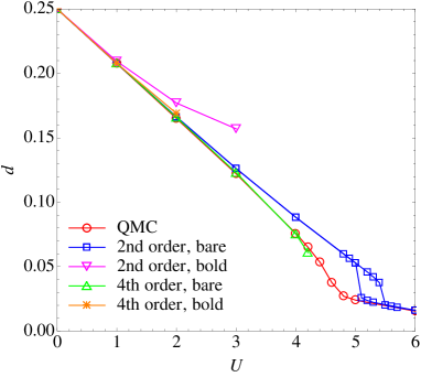
Figure 6: (Color online) The double occupancy for the Hubbard model in equilibrium at half filling with $\beta=16$ calculated from DMFT with various impurity solvers.

Away from half filling, we calculate the density per spin, $n=G^{M}(0^{-})$, as a function of $U$ for a fixed chemical potential $\mu-U/2=0.5,1,2$. The results obtained by DMFT with QMC, the Hartree approximation, and the second-order perturbation theories are shown in Fig. 7, while the results from the third-order perturbation expansions are shown in Fig. 8. We consider five types of perturbation expansions (I)-(V) as indicated in Table 1. The QMC results indicate that there are Mott transitions in the strong $U$ regime (e.g., $U_{c}\sim 6$ for $\mu-U/2=1$), where the density $n$ approaches 0.5. The Hartree approximation (dashed line in Fig. 7), which only includes the Hartree term (30) as the self-energy correction, deviates from QMC already at relatively small $U$ $(\sim 1)$. Among the various second-order expansions, type (IV) (bare second-order and bold Hartree diagrams with $\alpha_{\sigma}=n_{\sigma}$) seems to be closest to the QMC result up to $U\sim 2.5$ for $\mu-U/2=0.5,1$ and $U\sim 4$ for $\mu-U/2=2$. However, this approach, as well as types (III) and (V), leads to a convergence problem in the DMFT calculation as one goes to larger $U$ [which is why the lines for types (III)-(V) in Figs. 7 and 8 are terminated]. On the other hand, type (I) easily converges even for large $U$.

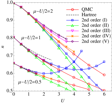
Figure 7: (Color online) The density for the Hubbard model in equilibrium with $\beta=16$ calculated by DMFT with QMC, Hartree approximation, and the second-order perturbation theories. The labels (I)-(V) correspond to the classification in Table 1.

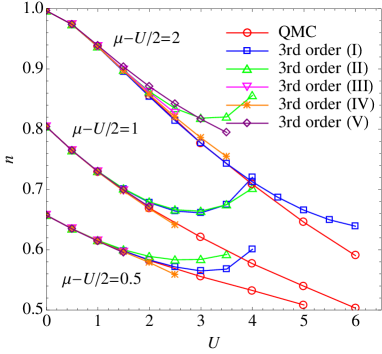
Figure 8: (Color online) The density for the Hubbard model in equilibrium with $\beta=16$ calculated by DMFT with the third-order perturbation theories. The labels (I)-(V) correspond to the classification in Table 1.

By comparing the second- (Fig. 7) and third-order (Fig. 8) perturbation theories, we see a systematic improvement of the results in most cases. In particular, the third-order type (I) becomes better than type (IV) and gets closest to QMC for $\mu-U/2=2$. It agrees with QMC up to $U\sim 4$. Again type (I) shows excellent convergence for the entire $U$ range, in contrast to the other approaches. For $\mu-U/2=1$, the results of type (I) are not improved from second to third order, while other types fail to converge around $U\approx 2.5$. Thus, it remains difficult to access the intermediate filling regime ($0.1<|n-0.5|<0.2,U>2$) using these weak-coupling perturbation expansions. If one goes far away from half filling (dilute regime), the system effectively behaves as a weakly correlated metal, and the perturbative approximations become valid.

Let us remark that it was pointed out earlier by Yosida and Yamada Yos that the bare weak-coupling perturbation theory is well behaved for the Anderson impurity model if it is expanded around the nonmagnetic Hartree solution. This corresponds to the expansion of type (IV) ($\alpha_{\sigma}=n_{\sigma}$) in our classification (Table. 1). Thus, their observation is consistent with our conclusion that type (IV) is as good as type (I) and is better than the other schemes. The difference is that when type (IV) expansion is applied to DMFT, it suffers from a convergence problem in the intermediate-coupling regime.

IV.2 Antiferromagnetic phase

Next, we test the validity of the perturbative impurity solvers for the equilibrium AFM phase of the Hubbard model at half filling. We show the AFM phase diagram in the weak-coupling regime obtained from DMFT with QMC, the Hartree approximation, and the second-order perturbation theories in Fig. 9. We also depict the phase diagram covering the entire $U$ range in Fig. 10. QMC provides the exact critical temperature $T_{c}$, which in the small-$U$ limit behaves as $T_{c}\propto v_{\ast}e^{-1/D(\epsilon_{F})U}$ [similar to the BCS formula for the superconducting phase; $D(\epsilon_{F})$ is the DOS at the Fermi energy]. $T_{c}$ takes the maximum value at $U\approx 4$ and slowly decays as $T_{c}\propto v_{\ast}^{2}/U$ in the strong-coupling regime. This is analogous to the BCS-BEC crossover for superconductivity which is often discussed in the context of cold-atom systems. Here, it corresponds to a crossover from the spin density wave in the weak-coupling regime to the AFM Mott insulator with local magnetic moments in the strong-coupling regime.

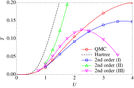
Figure 9: (Color online) The AFM transition temperature for the Hubbard model at half filling derived from DMFT with various impurity solvers. The region below (above) the curves represents the AFM (PM) phase. The labels (I)-(III) correspond to the classification in Table 1. The QMC data are taken from Ref. Koga and Werner, 2011.

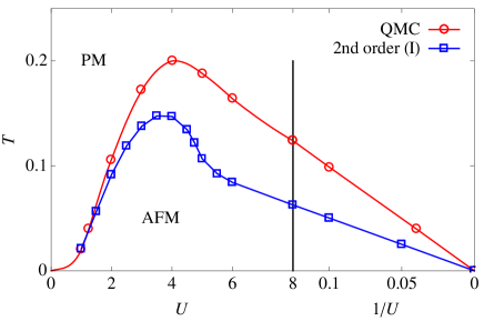
Figure 10: (Color online) The AFM phase diagram of the Hubbard model covering the weak-coupling and strong-coupling limits. The QMC data are taken from Ref. Koga and Werner, 2011.

The Hartree approximation (dashed curve in Fig. 9) correctly reproduces the weak-coupling asymptotic form, $T_{c}\propto v_{\ast}e^{-1/D(\epsilon_{F})U}$, but starts to deviate from the QMC result already at $U\sim 0.5$. The second-order perturbation theories of types (I)-(III) give better results than the Hartree approximation as shown in Fig. 9. However, quantitatively the agreement with QMC is still not so good for $U>1$. This problem was previously pointed out for the second-order perturbation expansion of type (III).Georges et al. (1996) We have not plotted $T_{c}$ estimated from the second-order perturbations of types (IV) and (V), since type (IV) gives a discontinuous (first-order) phase transition which is not correct for the AFM order, and type (V) yields a pathological discontinuous jump of the magnetization as a function of temperature within the ordered phase which is physically unreasonable.

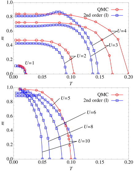
Figure 11: (Color online) The staggered magnetization for the Hubbard model at half filling evaluated by DMFT with QMC and the second-order perturbation theory of type (I) in the weak-coupling (top panel) and strong-coupling (bottom panel) regimes. The QMC data for $U=2,10$ are taken from Ref. Koga and Werner, 2011.

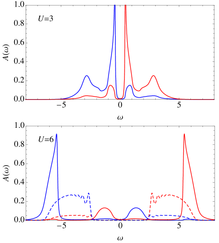
Figure 12: (Color online) The spectral function of the majority (minority) spin component [blue (red) solid curve] for the AFM phase of the Hubbard model at half filling calculated by DMFT with the second-order perturbation theory of type (I). The dashed lines show the spectral function calculated by DMFT with the noncrossing approximation. The parameters are $U=3,\beta=20$ (top panel) and $U=6,\beta=16$ (bottom).

Type (I) continues to converge in the strong-coupling regime, in contrast to other second-order approaches that fail to converge at some point. What is special about this weak-coupling expansion is that it qualitatively captures the BCS-BEC crossover; i.e., the critical temperature scales appropriately both in the weak- and strong-coupling limits (Fig. 10). Quantitatively, the value of $T_{c}$ given by the type (I) second-order scheme is roughly a factor of 2 lower than the QMC result in the large-$U$ regime. If one restricts the DMFT solution to the PM phase, it is known that the second-order bare-diagram expansion (IPT) reproduces the correct strong-coupling limit. The AFM critical temperature, on the other hand, depends on the treatment of the Hartree term (note that even in the PM phase the evaluation of the spin susceptibility may depend on the choice of the Hartree diagram since it enters in the vertex correction), and only the approach of type (I) among the various methods that we tested survives for large $U$. It would be interesting to compare the situation with the $T$-matrix approximationKeller et al. (1999, 2001) that is often adopted in the study of the attractive Hubbard model. It takes account of a series of ladder diagrams for the self-energy and similarly reproduces the BCS-BEC crossover for $T_{c}$.

We also plot the staggered magnetization $m=\sum_{\sigma}\sigma n_{\sigma}=\sum_{\sigma}\sigma G_{\sigma}^{M}(0^{-})$ for the ordered state evaluated by QMC and the second-order perturbation theory of type (I) in the weak-coupling (the top panel of Fig. 11) and strong-coupling (bottom panel) regimes. For small $U$, the second-order perturbation theory gives a smooth curve for the magnetization as a function of $T$. As one increases $U$, there emerges a kink in the magnetization curve for $U\geq 4$ (Fig. 11), which is an artifact of the perturbation theory as confirmed by comparison to the QMC results. Hence, although $T_{c}$ behaves reasonably in the large $U$ regime, it is unlikely that the second order perturbation of type (I) correctly describes the strong-coupling state.

Figure 12 plots the spectral function $A_{\sigma}(\omega)=-\frac{1}{\pi}{\rm Im}G_{\sigma}^{R}(\omega)$ obtained from the second-order perturbation of type (I). The weak-coupling regime ($U=3$, top panel of Fig. 12) shows coherence peaks separated by the AFM energy gap and accompanied by the Hubbard sidebands. However, as one goes to the strong-coupling regime ($U=6$, bottom panel of Fig. 12), the coherence peaks are rapidly shifted away from the Fermi energy, and two additional bands appear around $\omega=\pm 1.5$. This is quite different from the result of the noncrossing approximationWerner et al. (2012) (dashed lines in the bottom panel of Fig. 12), which is supposed to be reliable in the strong-coupling regime, and shows spin-polaron peaks on top of the Mott-Hubbard bands with a large energy gap. Therefore, we conclude that the second-order perturbation of type (I) does not correctly describe the AFM state in the strong-coupling regime.

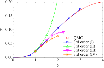
Figure 13: (Color online) The AFM transition temperature for the Hubbard model at half filling derived from DMFT with various third-order perturbation impurity solvers. The region below (above) the curves represents the AFM (PM) phase. The labels (I)-(IV) correspond to the classification in Table 1.

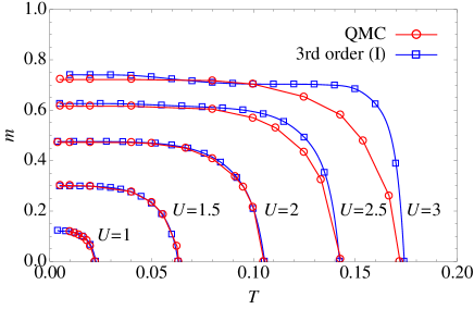
Figure 14: (Color online) The staggered magnetization of the Hubbard model at half filling evaluated by DMFT with QMC and the third-order perturbation theory of type (I).

The phase diagram derived from DMFT using various third-order perturbation theories is shown in Fig. 13. Again we do not draw the $T_{c}$ curve for type (V), since it has a discontinuous jump of the magnetization as a function of temperature in the ordered state. We find that the third-order perturbation of type (I) (all the diagrams including the Hartree term are bare) reproduces $T_{c}$ very accurately up to $U=3$. A comparable accuracy cannot be obtained with the other third-order expansions. To establish the validity of this approach, we calculate the staggered magnetization below $T_{c}$, which is illustrated in Fig. 14. By comparing the results with those of QMC, we can see that the type (I) third-order approach predicts not only accurate $T_{c}$ but also correct magnetizations for $U\leq 2.5$.Tsuji et al. (2013) When $U$ becomes larger than 2.5, deviations from the exact QMC results start to appear, and the curvature of the magnetization curve gets steeper. Thus, the third-order perturbation of type (I) is the method of choice for studying the AFM phase in the weak-coupling regime ($U<3$). This is again consistent with the observation of Yosida and Yamada Yos that the bare weak-coupling expansion works well if expanded around the nonmagnetic Hartree solution (i.e., $\alpha_{\sigma}=\frac{1}{2}$).

V Interaction quench in the paramagnetic phase of the Hubbard model

Having examined the performance of the weak-coupling perturbation theories for the equilibrium state of the Hubbard model, we move on to studying the validity of the perturbative methods for nonequilibrium problems. In this section, we focus on the interaction quench problem for the PM phase of the Hubbard model; i.e., we consider the Hamiltonian (1) with the interaction parameter abruptly varied as

$$U(t)=\begin{cases}U_{i}&t=0^{-}\\ U_{f}&t>0\end{cases}.$$ (54)

The interaction quench problem for the Hubbard model has been previously studied using the flow equation and unitary perturbation theory,Moeckel and Kehrein (2008, 2010) nonequilibrium DMFT,Eckstein et al. (2009, 2010) time-dependent Gutzwiller variational method,Schiró and Fabrizio (2010, 2011) generalized Gibbs ensemble,Kollar et al. (2011) equation-of-motion approach,Hamerla and Uhrig (2013, ) and quantum kinetic equation.Stark and Kollar In the weak-coupling regime, the physics of “prethermalization”Berges et al. (2004) has been discussed.

Here we take the parameters, $U_{i}=0$ (noninteracting initial state) and the initial temperature $T=0$, to allow a systematic comparison with these previous results. We use the second-order and fourth-order perturbation theories for the half-filling case in Sec. V.1 and the third-order perturbation theory for calculations away from half filling in Sec. V.2. We restrict ourselves to the PM solution of the nonequilibrium DMFT equations throughout this section.

V.1 Half filling

To study the relaxation behavior of the Hubbard model after the interaction quench, we calculate the time evolution of the double occupancy $d(t)=\langle n_{\uparrow}(t)n_{\downarrow}(t)\rangle$ within nonequilibrium DMFT via the formula,

$$d(t)=-\frac{i}{2U}\sum_{\sigma}(\Sigma_{\sigma}\ast G_{\sigma})^{<}(t,t),$$ (55)

which can be derived from the equation of motion. Initially the system is noninteracting, so that $d(0^{-})=\langle n_{\uparrow}\rangle\langle n_{\downarrow}\rangle=1/2\times 1/2=1/4$ at half filling. The results for $d(t)$ obtained with different impurity solvers (QMC, bare second-order, and bare fourth-order perturbation theory) are plotted for $U_{f}\leq 3$ in the top panel of Fig. 15. As one can see, the results of the second and fourth order agree very well with the QMC results up to $U_{f}=1.5$. After the quench, the double occupancy quickly relaxes to an almost constant value, which is quite close to the thermal value of the final state. Eckstein et al. (2009) At $U_{f}=2$ and $2.5$, the difference between the second and fourth order becomes larger, and the latter reproduces the correct result of the double occupancy with an irregular hump around $t\sim 2.5$. The second-order perturbation predicts an overdamping of the double occupancy without a hump.

The results for the double occupancy in the intermediate- and strong-coupling regimes ($4\leq U_{f}\leq 8$) are shown in the top panel of Fig. 16. As we increase the interaction strength, the perturbation theories quickly deviate from the QMC results, and an agreement is found only on very short time scales. The fourth-order expansion thus fails to improve the second-order results in this regime, and seems to be numerically more unstable than the second order. We discuss later that this is related to pathological violation of energy conservation.

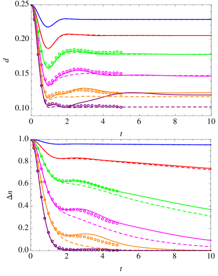
Figure 15: (Color online) Time evolution of the double occupancy (top panel) and the jump of the momentum distribution function (bottom panel) after the interaction quenches $U=0\to 0.5,1,\dots,3$ (from top to bottom) in the PM phase of the Hubbard model at half filling calculated by the nonequilibrium DMFT with QMC (circles, taken from Ref. Eckstein et al., 2009), the bare second-order (dashed curves), and bare fourth-order (solid curves) perturbation theories.

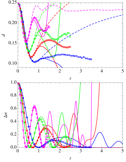
Figure 16: (Color online) Time evolution of the double occupancy (top panel) and the jump of the momentum distribution function (bottom) after the interaction quenches $U=0\to 4,5,6,8$ (from bottom to top in the first minima of $d$, and from top to bottom in the initial decrease of $\Delta n$) in the PM phase of the Hubbard model at half filling calculated by the nonequilibrium DMFT with QMC (circles, taken from Ref. Eckstein et al., 2009), the bare second-order (dashed curves), and bare fourth-order (solid curves) perturbation theories.

We also compute the momentum distribution,

$$n_{\boldsymbol{k}}(t)=-iG_{\boldsymbol{k}}^{<}(t,t).$$ (56)

The distribution of the initial noninteracting state at $T=0$ is $n_{\boldsymbol{k}}=\theta(\mu-\epsilon_{\boldsymbol{k}})$, which has a discontinuous jump $\Delta n=1$ at the Fermi energy. This jump does not immediately disappear after the quench, but survives for some period.Eckstein et al. (2009) It is a measure of how close or far the system is from the thermalized state. If the system fully thermalizes after the quench, the jump $\Delta n$ should vanish since a thermal state at nonzero temperature has a smooth distribution. In the bottom panel of Fig. 15, we show the time evolution of $\Delta n$ obtained by the nonequilibrium DMFT with QMC, bare second-order and bare fourth-order perturbations for $U_{f}\leq 3$. The QMC results suggest that, in contrast to the double occupancy, $\Delta n$ does not directly relax to the thermal value ($\Delta n=0$), but is trapped at some intermediate value for some time. Although local quantities such as the double occupancy look thermalized at this moment (prethermalization), the distribution is clearly nonthermal. Moeckel and Kehrein (2008) After prethermalization, $\Delta n$ slowly relaxes to zero. The time scale of this relaxation is much longer than that for the double occupancy.

The difference between the second- and fourth-order perturbations for $\Delta n$ is clearer than in the case of the double occupancy. It already becomes evident at $U_{f}=1.5$. Before $\Delta n$ approaches the plateau ($t<1.5$), both methods give almost the same results. However, the second-order results do not show a clear plateaulike structure in the prethermalization regime ($1.5\lesssim t\lesssim 3$), while the fourth order does. One can see in the bottom panel of Fig. 15 that the results of the fourth-order perturbation theory for $\Delta n$ agree fairly well with those of QMC for $U_{f}\leq 3$.

We also show the results for $\Delta n$ in the intermediate- and strong-coupling regimes ($4\leq U_{f}\leq 8$) in the bottom panel of Fig. 16. It has been known that the behavior of $\Delta n$ qualitatively changes from the weak- to the strong-coupling regime near $U_{c}^{\rm dyn}=3.2$ (dynamical transition). Eckstein et al. (2009); Schiró and Fabrizio (2010) On the weak-coupling side $\Delta n$ monotonically decays without touching zero, while on the strong-coupling side $\Delta n$ oscillates between zero and nonzero values. One can see that the bare perturbation theories (both second and fourth order) correctly reproduce the short-time dynamics of these collapse-and-revival oscillations in $\Delta n$ with period $2\pi/U$. Especially, they capture the sharp qualitative change of the short-time behavior of $\Delta n$. In the second-order perturbation theory the oscillations of $\Delta n$ always damp faster than those given by the fourth-order calculation. Similarly to the double occupancy, the $\Delta n$ obtained from the perturbation theories fail to reproduce the QMC results after the second- and fourth-order calculations start to deviate with each other.

The quality of the bare-diagram perturbation theory can be judged by looking at the evolution of the total energy (Fig. 17). The total energy of the Hubbard model is given by

$$E(t)=\sum_{\boldsymbol{k}\sigma}\epsilon_{\boldsymbol{k}}n_{\boldsymbol{k}\sigma}(t,t)+U(t)\left(d(t)-\frac{1}{4}\right).$$ (57)

For the semicircular DOS in the PM and AFM phases, the kinetic-energy term can be rewritten in terms of the local Green’s functions as

$$\sum_{\boldsymbol{k}\sigma}\epsilon_{\boldsymbol{k}}n_{\boldsymbol{k}\sigma}(t,t) =-i\sum_{\sigma}(\Delta_{\sigma}\ast G_{\sigma})^{<}(t,t)$$

$$=-iv_{\ast}^{2}\sum_{\sigma}(G_{\overline{\sigma}}\ast G_{\sigma})^{<}(t,t).$$ (58)

Since the bare-diagram expansions are not a conserving approximation, it is not guaranteed that the total energy is conserved after the quench, even though the Hamiltonian becomes time independent. To make a systematic comparison, we consider the difference between $E(t>0)$ and $E(0^{+})$, which should be zero if the total energy is indeed conserved. As one can see in Fig. 17, the total energy is nicely conserved up to $U_{f}=2$. However, when $U_{f}$ exceeds $2$, the conservation of the total energy is suddenly violated for both the second-order and the fourth-order perturbation theories [the drift in total energy is smaller in the second-order perturbation]. In particular, the fourth-order expansion does not extend the interaction region in which the total energy is conserved. If one compares the energy drift at $t=5$ and $t=10$ in Fig. 17, one sees that the drift is “saturated” for $U_{f}\leq 3$ at the second order and for $U_{f}\leq 2$ at the fourth order; i.e., the drift only occurs on a certain short time scale and the difference to the correct total energy does not grow anymore thereafter. In other words, the bare perturbation theory “does not accumulate” numerical errors as time evolves for $U_{f}\leq 2$. From this, we can conclude that the bare perturbation theories remain reliable up to long times for these $U_{f}$, which is a big advantage of this approach.

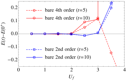
Figure 17: (Color online) The drift of the total energy $E(t)-E(0^{+})$ (measured at $t=5,10$) in the simulation of the interaction quench $U=0\to U_{f}$ using the bare second-order and bare fourth-order perturbation solvers.

The breakdown of the total-energy conservation generically implies a deviation of the results for $d$ or $\Delta n$ from QMC in the regime $U_{f}>2$ (Figs. 15 and 16). Let us remark that this does not necessarily mean that the bare perturbation theory always fails to describe the dynamics of the Hubbard model with $U>2$. It all depends on how the system is perturbed (interaction quench, slow ramp, electric-field excitation, etc.), the initial state (noninteracting or interacting), and other details of the problem. The general tendency is that the total energy is conserved when the excitation energy is small and/or the interaction strength is weak.

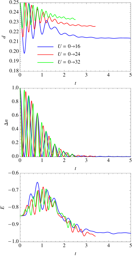
Figure 18: (Color online) Time evolution of the double occupancy (top), the jump of the momentum distribution function (middle), and the total energy (bottom) after the interaction quenches $U=0\to 16,24,32$ (from long- to short-time data) in the PM phase of the Hubbard model at half filling calculated by nonequilibrium DMFT with the bare second-order perturbation theory.

If we further increase $U_{f}$, the second-order bare perturbation theory again starts to work reasonably well. In Fig. 18, we plot $d$, $\Delta n$, and $E$ for quenches $U=0\to 16,24,32$. The simulation is numerically stable within the accessible time range, and the observables do not diverge as time grows. The results nicely show the coherent collapse-and-revival oscillations of period $2\pi/U$, which are characteristic of the atomic limit. We also observe that the envelope curve of rapidly oscillating $\Delta n$ is “universal”; i.e., it is almost invariant against large enough $U$. In contrast, the fourth-order bare perturbation theory fails to produce physically reasonable results for these $U$. The seeming success of the second-order bare perturbation theory (IPT) for very large $U$ appears to be related to the fact that IPT reproduces the correct atomic limit of the Hubbard model in equilibrium.Georges et al. (1996) However, it is a priori not obvious that IPT also describes the correct nonequilibrium dynamics near the atomic limit, since the dynamics here starts from the noninteracting state which is very far from the atomic limit, and errors can accumulate in the strong-coupling regime as the system time evolves. Indeed, if one looks at the total energy $E$ (bottom panel of Fig. 18), there is a non-negligible energy drift whose magnitude ($\sim 10\%$ of the absolute value of $E$) is roughly independent of $U$. Despite the violation of energy conservation, IPT seems to work surprisingly well out of equilibrium near the atomic limit.

We have also tested the second-order and fourth-order self-consistent perturbation theories (bold-diagram expansions). The results for the double occupancy and the jump in the momentum distribution for $U_{f}\leq 3$ ($U_{f}\geq 4$) are shown in the top and bottom panels of Fig. 19 (Fig. 20), respectively. By comparing with QMC, one can see that the self-consistent perturbation theories are not particularly good. Although we have a slight improvement from the second-order to the fourth-order expansion, a deviation from the QMC results still remains, even in the short-time dynamics. The detailed dynamics of $d$ and $\Delta n$ in the transient and long-time regimes is not correctly reproduced. The damping of the double occupancy is too strong in both the weak-coupling and the strong-coupling regimes (see also Ref. Eckstein et al., 2009). This may be due to a too-tight self-consistency condition, i.e., the self-consistency within the perturbation theory and the DMFT self-consistency. [Flaws in the (second-order) self-consistent perturbation theory, when applied to the equilibrium DMFT,Müller-Hartmann (1989) were pointed out already in Ref. Georges and Kotliar, 1992. In particular, it was noted that it does not reproduce the high-energy features (Hubbard sidebands) of the spectral function.] For $\Delta n$, the height of the prethermalization plateau is not correctly reproduced for $U_{f}\leq 3$. On the strong-coupling side, $\Delta n$ relaxes monotonically without showing any oscillation. This evidences that the self-consistent perturbation theory cannot describe the dynamical transition found in the interaction-quenched Hubbard model at half filling. Eckstein et al. (2009); Schiró and Fabrizio (2010) Hence, even though the self-consistent perturbation theory is a conserving approximation, it is not the impurity solver of choice for nonequilibrium DMFT.

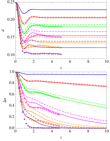
Figure 19: (Color online) Time evolution of the double occupancy (top panel) and the jump of the momentum distribution function (bottom) after the interaction quenches $U=0\to 0.5,1,\dots,3$ (from top to bottom) in the PM phase of the Hubbard model at half filling calculated by the nonequilibrium DMFT with QMC (circules, taken from Ref. Eckstein et al., 2009), the bold second-order (dashed curves), and the bold fourth-order (solid curves) self-consistent perturbation theories.

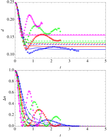
Figure 20: (Color online) Time evolution of the double occupancy (top panel) and the jump of the momentum distribution function (bottom) after the interaction quenches $U=4,5,6,8$ (from bottom to top in the long-time limit of $d$, and from top to bottom in $\Delta n$) in the PM phase of the Hubbard model at half filling calculated by the nonequilibrium DMFT with QMC (circules, taken from Ref. Eckstein et al., 2009), the bold second-order (dashed curves), and the bold fourth-order (solid curves) self-consistent perturbation theories.

V.2 Away from half filling

When the filling is shifted away from half filling, the particle-hole symmetry is lost, and odd-order diagrams start to contribute in the calculation. Here we consider the interaction quench problem for the PM phase of the Hubbard model at quarter filling, i.e., $n_{\sigma}=1/4$, and apply the second-order and third-order perturbation theories. We adopt the type (I) and type (IV) approaches in the classification of Table 1, i.e., the bare-diagram expansions having the bare tadpole diagram with $\alpha_{\sigma}=1/2$ and bold tadpole with $\alpha_{\sigma}=n_{\sigma}$, since they have been shown to be relatively good approximations away from half filling in Sec. IV.1.

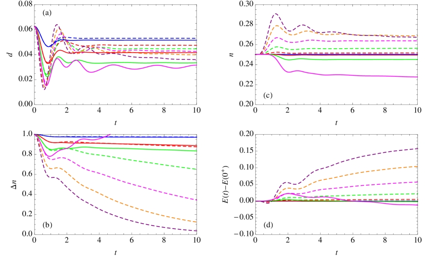
Figure 21: (Color online) Time evolution of the double occupancy (a), the jump of the momentum distribution function (b), the density (c), and the total-energy drift (d) after interaction quenches in the PM phase of the Hubbard model at quarter filling calculated by the nonequilibrium DMFT with the type (I) second-order (dashed curves, $U=0\to 0.5,1,\dots,3$), and type (I) third-order (solid curves, $U=0\to 0.5,1,1.5,2$) perturbation theories.

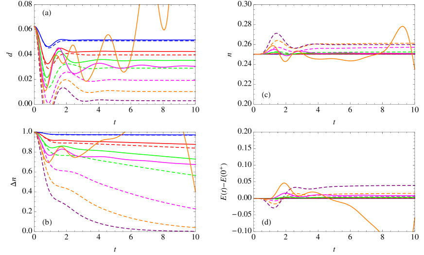
Figure 22: (Color online) Time evolution of the double occupancy (a), the jump of the momentum distribution function (b), the density (c), and the total-energy drift (d) after interaction quenches in the PM phase of the Hubbard model at quarter filling calculated by the nonequilibrium DMFT with the type (IV) second-order (dashed curves, $U=0\to 0.5,1,\dots,3$), and type (IV) third-order (solid curves, $U=0\to 0.5,1,\dots,2.5$) perturbation theories.

We plot the results produced by the type (I) and type (IV) expansions in Figs. 21 and 22, respectively. In Fig. 21(a), we show the time evolution of the double occupancy calculated by the type (I) scheme. The noninteracting initial state has $d(0)=1/4\times 1/4=1/16=0.0625$. The second-order and third-order perturbations give quantitatively different evolutions after the quench. When $U_{f}$ is small enough ($U_{f}\leq 1$), the double occupancy quickly damps to a thermal value. As one increases $U_{f}$, an enhanced oscillation starts to appear in both the second-order and the third-order calculations. In Fig. 21(b), we plot the time evolution of the jump $\Delta n$ at the Fermi energy in the momentum distribution. Initially, the system has a Fermi distribution with $T=0$, so that $\Delta n(0)=1$. The second-order calculations (dashed curves in the bottom panel of Fig. 21) show that after a rapid decrease, $\Delta n$ stabilizes at an intermediate value for a certain time and then slowly decays to zero. This behavior (prethermalization) is quite similar to what we have seen in the case of half filling. If we use the third-order perturbation theories, however, the results differ from those of the second order for $U_{f}\geq 1.5$. In particular, at $U_{f}=2$ the jump $\Delta n$ starts to oscillate and finally exceeds $1$, implying that the third-order calculation gives physically unreasonable results.

To examine the validity of the perturbation theories, we show the density and total energy as a function of time in Figs. 21(c) and 21(d). They should be conserved throughout the time evolution. The results suggest that the total energy and density ($n=1/4$) are reasonably conserved when $U_{f}\leq 1$ in both the second-order and the third-order perturbations. Only in this parameter regime, the simulation is reliable. This limitation is more severe than in the half-filling case, where the total energy is sufficiently conserved up to $U_{f}=2$.

We also investigated the type (IV) approach in Table 1 and show the results in Fig. 22. The behavior of $d$ and $\Delta n$ [Figs. 22(a) and 22(b)] looks qualitatively similar to the result of the type (I) expansion, while there are quantitative differences such as the value of $d$ after relaxation and the plateau height for $\Delta n$ in the prethermalization regime. The simulation with the third-order expansion of type (IV) becomes particularly unstable at $U_{f}=2.5$, showing rapid oscillations in $d$ and an irregular evolution in $\Delta n$. If one looks at the density and total energy given by the type (IV) perturbation [Figs. 22(c) and 22(d)], the conserving nature is somewhat improved with respect to the type (I) calculation. The conservation starts to break down earlier in $U_{f}$ in the third-order expansion compared to the second-order one. Thus, we do not see a systematic improvement away from half filling by proceeding to higher-order perturbation expansions. It should be noted that also the weak-coupling QMC method can only reach times which are about a factor of two shorter than in the case of half-filling, because the odd-order diagrams contribute to the sign problem. Hence, the development of a useful impurity solver for nonequilibrium DMFT calculations away from half filling in the weak-coupling regime remains an open issue.

VI Dynamical symmetry breaking induced by an interaction ramp in the Hubbard model

So far, we have considered the interaction quench dynamics of the Hubbard model without any long-range order. Since the formalism of the nonequilibrium DMFT has been generalized to the AFM phase in Sec. II, we can apply the perturbative impurity solvers to the dynamics of such an ordered state.

In this section, we study dynamical symmetry breaking in the Hubbard model induced by an interaction ramp by means of the nonequilibrium DMFT with the third-order perturbation theory of type (I) (Table 1). This impurity solver correctly reproduced the AFM phase diagram (Fig. 13) and the magnetization (Fig. 14) in the weak-coupling regime. We begin with the PM initial state in thermal equilibrium, and then change the interaction parameter continuously (ramp) as

$$U(t)=\begin{cases}U_{i}+(U_{f}-U_{i})t/t_{\rm ramp}&0\leq t\leq t_{\rm ramp},\\ U_{f}&t>t_{\rm ramp},\end{cases}$$ (59)

where $t_{\rm ramp}$ is the ramp time, to go across the phase transition line in the phase digram (Fig. 13). We consider an interaction ramp ($t_{\rm ramp}>0$) rather than a quench ($t_{\rm ramp}=0$) to reduce the increase of the energy, but it turns out that the results do not significantly depend on $t_{\rm ramp}$.

In order to trigger the symmetry breaking, we introduce a tiny staggered magnetic field $h$ in the initial state. We assume that the seed field $h$ is uniform in space, so that the order parameter (staggered magnetization $m$) grows uniformly. From a large-scale point of view, this assumption is probably not appropriate, since the direction of symmetry breaking is random at each position, which leads to domain structures and topological defects in between (Kibble-Zurek scenario Kibble (1976); Zurek (1985)). However, our interest here lies in the fast microscopic dynamics of the order parameter, where our set up can be justified. For convenience, we ramp off the seed field in the following way:

$$h(t)=\begin{cases}h(1-t/t_{\rm ramp})&0\leq t\leq t_{\rm ramp},\\ 0&t>t_{\rm ramp}.\end{cases}$$ (60)

VI.1 Nonequilibrium DMFT results

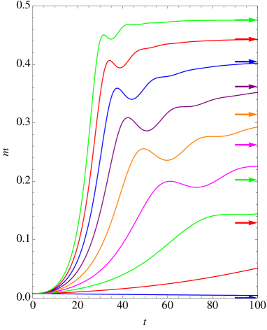
Figure 23: (Color online) Time evolution of the staggered magnetization after the interaction ramps $U=1.75\to 1.8,1.9,\dots,2.6$ (from bottom to top) in the Hubbard model. $\beta=11$, $h=10^{-4}$, and $t_{\rm ramp}=10$. The arrows indicate the corresponding thermal values reached in the long-time limit.

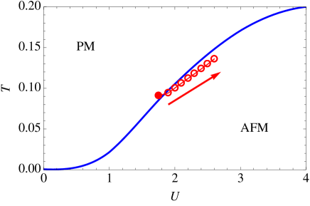
Figure 24: (Color online) The initial (solid circle, $U_{i}=1.75$) and final (open circles, $U_{f}=1.9,2,\dots,2.6$ from left to right) thermal states in the simulation of the dynamical symmetry breaking in Fig. 23. The labels “PM” and “AFM” indicate the paramagnetic and antiferromagnetic phases, respectively.

In Fig. 23, we show the evolution of the staggered magnetization after the interaction ramp obtained by the nonequilibrium DMFT. The parameters are chosen such that $U_{i}=1.75$, $\beta=11$, $h=10^{-4}$, and $t_{\rm ramp}=10$. The initial state is in the PM phase and is quite close to the AFM phase boundary (solid red circle in Fig. 24). We fix the initial state and systematically change $U_{f}$ to perform a series of interaction-ramp simulations. The initial magnetization is very small but finite due to the presence of the staggered magnetic field $h$. After the interaction ramp, the PM state becomes unstable, and the order parameter starts to grow exponentially ($m\propto e^{t/\tau_{i}}$ with $\tau_{i}$ the initial growth rate). It is followed by an amplitude oscillation and a gradual relaxation toward the final state. Here the oscillation is not as coherent as in the case of a ramp out of the symmetry-broken phase,Tsuji et al. (2013) and one can see a softening of the amplitude mode in Fig. 23.

In the long-time limit, the system finally thermalizes in the nonintegrable Hubbard model. We can estimate the final temperature by searching for the equilibrium thermal state with effective temperature $T_{\rm eff}$ that has the same total energy as the time-evolving state, since the total energy should be conserved after the interaction ramp. In Fig. 25, we plot the total energy for the interaction ramps that correspond to Fig. 23. For $U_{f}\lesssim 2.1$, the total energy is nicely conserved after the interaction ramps. As $U_{f}$ is further increased, there emerges a small energy drift during the symmetry breaking ($10\leq t\lesssim 40$). After the symmetry breaking, the conservation of the total energy is recovered. Thus, we have a slight inaccuracy in the simulation of the interaction ramps for larger $U_{f}$. We use the final value of the total energy, $E_{\rm tot}(t=100)$, to extract the effective temperature of the thermal states reached in the long-time limit. In Fig. 24, we indicate the final thermalized states in the phase diagram by open circles. As we increase $U_{f}$, $T_{\rm eff}$ increases in the vicinity of the phase boundary. Similarly to the case of the dynamical phase transition out of the AFM phase,Tsuji et al. (2013) it seems to trace more or less the constant entropy curve,Werner et al. (2005) although the interaction ramps that we consider here are not at all adiabatic processes.

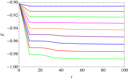
Figure 25: (Color online) Time evolution of the total energy for the interaction ramps that correspond to Fig. 23.

The arrows in Fig. 23 indicate the thermal value of the order parameter ($m_{\rm th}$) that is realized in the long-time limit. We notice that there is a large deviation between the transient magnetization and the thermal values $m_{\rm th}$ for $1.9\leq U_{f}\leq 2.2$. Especially, the center of the oscillation of the amplitude mode is different from the long-time limit $m_{\rm th}$, so that the evolution of the order parameter is a superposition of a damped oscillation and a slow drift. This reminds us of the behavior of the order parameter seen in the dynamical phase transition from the AFM to PM phase induced by an interaction ramp,Tsuji et al. (2013) where $m$ does not decay immediately after the ramp but is “trapped” to a nonthermal value for a long time. It has been shown for that case that on a relatively short time scale the order-parameter dynamics is governed by the presence of a “nonthermal critical point,” in the vicinity of which the period of the amplitude mode diverges.

One may define two time scales that characterize the trapping of the nonthermal fixed point, namely the “approach time” to and the “escape time” from the nonthermal fixed point. The escape time is determined by $U_{f}$. In the $U_{f}\to 0$ limit it diverges to infinity, while for $U_{f}\to 3$ it becomes quite short (Fig. 23) since thermalization is accelerated. This is consistent with the previous observation of fast thermalization in the PM phase of the Hubbard model.Eckstein et al. (2009) On the other hand, the characterization of the approach time is unclear because it depends on the definition. If one considers the initial exponential growth of the order parameter as part of the nonthermal fixed-point behavior, then the approach time is very short and does not significantly depend on $U_{i}$ and $U_{f}$. Indeed, as we see in Sec. VI.3, this exponential growth exists in the Hartree solution, which characterizes the nonthermal fixed point. The weak dependence of the approach time on $U$ is consistent with Refs. Moeckel and Kehrein, 2008 and Eckstein et al., 2009. However, if one interprets the approach time as the time necessary for the order parameter to enter the coherently oscillating regime, then it is roughly determined by $\tau_{i}$.

To analyze the critical behavior of the dynamical symmetry breaking near the phase transition point, we plot several relevant quantities in Fig. 26. $m_{\rm th}$ (the thermal value reached in the long-time limit) vanishes at the thermal critical point ($U_{f}=U_{c}^{\rm th}$) as

$$m_{\rm th}\sim(U_{f}-U_{c}^{\rm th})^{\frac{1}{2}}.$$ (61)

This is consistent with the mean-field prediction $m_{\rm th}\sim(U_{f}-U_{c}^{\rm th})^{\beta}$ with the mean-field critical exponent $\beta=\frac{1}{2}$. $\tau_{i}$ is the time constant of the initial exponential growth ($m\propto e^{t/\tau_{i}}$), which diverges as

$$\tau_{i}\sim(U_{f}-U_{c}^{\rm th})^{-1}.$$ (62)

Note that these exponents are universal; i.e., they do not depend on details of the problem (the initial condition, perturbation of the system, etc.). We also measured the maximum of the first peak ($m_{\rm max}$) and the minimum of the first dip ($m_{\rm min}$) of the amplitude oscillation, and we plot these quantities in Fig. 26. $m_{\rm max}$ and $m_{\rm min}$ characterize the “trapping” of the order parameter in the transient regime. They behave differently from $m_{\rm th}$: $m_{\rm max}$ and $m_{\rm min}$ are always smaller than $m_{\rm th}$. The middle point $m_{\rm nth}\equiv(m_{\rm max}+m_{\rm min})/2$ (nonthermal magnetization) seems to depend linearly on $U_{f}$, which must be contrasted with the square-root dependence for $m_{\rm th}$ (61). We see in Sec. VI.3 that this linear scaling can be justified in the weak-correlation limit. The linear extrapolation of the middle points (dashed line in Fig. 26) implies that the trapped order parameter vanishes at a certain point $U_{f}=U_{\ast}^{\rm nth}$, which is different from the thermal critical point ($U_{f}=U_{c}^{\rm th}$), as

$$m_{\rm nth}\sim(U_{f}-U_{\ast}^{\rm nth})^{1}.$$ (63)

As we see later in Sec. VI.3, this nonthermal critical behavior becomes “exact” in the small $U$ regime (where the Hartree approximation is applicable) with $U_{\ast}^{\rm nth}$ identical to $U_{c}^{\rm th}$. There are several possible interpretations of the behavior (63) for larger $U$: One is that the nonthermal critical point is shifted from $U_{f}=U_{c}^{\rm th}$ to $U_{\ast}^{\rm nth}$ due to correlation effects. Another interpretation is that the nonthermal critical point still exists at $U_{f}=U_{c}^{\rm th}$, but $m_{\rm max}$ and $m_{\rm min}$ are lifted up due to thermalization toward $m_{\rm th}$. In any case, it is likely that the qualitative features of the nonthermal critical point survive to some extent in the moderate $U$ regime, so that it affects the order-parameter dynamics during the dynamical symmetry breaking.

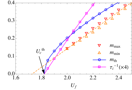
Figure 26: (Color online) Various quantities that characterize the critical behavior of the dynamical symmetry breaking with $U_{i}=1.75$: $m_{\rm max}$ and ($m_{\rm min}$) is the maximum (minimum) of the first cycle of the oscillation in $m(t)$, $m_{\rm th}$ is the thermal value taken in the long-time limit, and $\tau_{i}$ is the rate of the initial exponential growth. The dashed line is an extrapolation of the middle points of $m_{\rm max}$ and $m_{\rm min}$.

If we start with a smaller $U_{i}$, the amplitude mode induced by the interaction ramp becomes more coherent. In Fig. 27, we show the time evolution of $m$ for $U_{i}=1.25$, $U_{f}=2$, $\beta=22$, $h=10^{-4}$, and $t_{\rm ramp}=10$ (blue curve). We can clearly see many oscillation cycles. Again the oscillation center slowly drifts to the thermal value $m_{\rm th}$ (arrow in Fig. 27). Figure 28 illustrates the corresponding evolution of the double occupancy. After the ramp ($t=10$), the double occupancy quickly approaches the thermalized value within the PM phase indicated by the arrow on the left in Fig. 28. This suggests that the system prethermalizes within the PM phase before the dynamical symmetry breaking occurs. After the order parameter $m$ starts to grow, the double occupancy also oscillates along with the amplitude oscillation of $m$. In the same way as $m$, the double occupancy slowly approaches the thermal value for the AFM phase (the arrow on the right in Fig. 28).

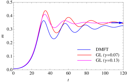
Figure 27: (Color online) Comparison between the DMFT result of $m(t)$ for the quench $U=1.25\to 2$, $\beta=22$ with the phenomenological Ginzburg-Landau theory. The arrow indicates the thermal value of $m$ reached in the long-time limit.

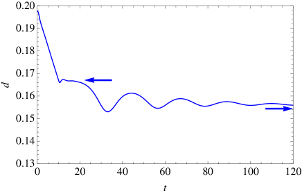
Figure 28: (Color online) The time evolution of the double occupancy for the quench $U=1.25\to 2$, $\beta=22$. The arrow on the left indicates the thermal value of $m$ for the PM phase, while the one on the right shows the value in the AFM phase.

The dynamics of the order parameter is reflected in the time-resolved spectral function $A_{\sigma}(\omega,t)$, which is defined by the retarded Green’s function,

$$A_{\sigma}(\omega,t)=-\frac{1}{\pi}{\rm Im}\int_{0}^{\infty}d\overline{t}\,e^{i\omega\overline{t}}G_{\sigma}^{R}(t+\overline{t}/2,t-\overline{t}/2).$$ (64)

This function represents the single-particle spectrum at time $t$. Since the range of the time arguments is limited ($\leq t_{\rm max}$), we have to introduce a cutoff in the semi-infinite integral in Eq. (64). As a result, the energy resolution $\Delta\omega$ is restricted (energy-time uncertainty). Here $\Delta\omega\sim 2\pi/t_{\rm max}\sim 0.06$, which is fine enough to resolve the AFM energy gap.

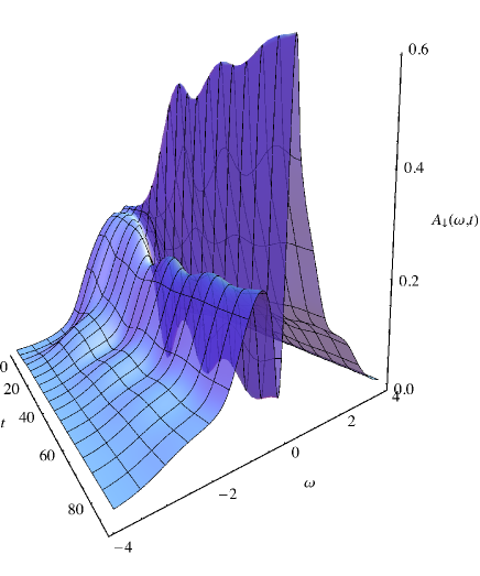
Figure 29: (Color online) The time-resolved spectral function $A(\omega,t)$ of the minority spin component for the quench $U=1.25\to 2$, $\beta=22$.

In Fig. 29, we depict $A_{\sigma}(\omega,t)$ for the interaction ramp ($U=1.25\to 2$) which corresponds to the blue magnetization curve in Fig. 27. At first, the system is noninteracting, so that $A_{\sigma}(\omega)=\sqrt{4v_{\ast}^{2}-\omega^{2}}/(2\pi v_{\ast}^{2})$ (noninteracting DOS). After the interaction ramp, an energy gap is dynamically generated at the Fermi energy ($\omega=0$) in the spectral function. Once the gap has opened, the magnitude of the gap [the distance between the coherence peaks in $A(\omega)$] stays nearly constant in time. On the other hand, there is a coherently oscillating spectral-weight transfer between the lower ($\omega<0$) and higher ($\omega>0$) energy region, consistent with the time-evolution of the order parameter $m$. The drift of the oscillation center is also reflected in $A(\omega,t)$. Therefore, the spectral function captures the characteristic behavior of the order-parameter dynamics. Experimentally, it is not easy to observe the time evolution of the staggered magnetization directly. However, the change of the spectral function can be detected by time-resolved photoemission spectroscopy and pump-probe optical spectroscopy. These techniques thus provide a way of tracking the evolution of the staggered magnetization.

VI.2 Comparison to the phenomenological Ginzburg-Landau equation

To analyze the behavior of the order parameter after the interaction ramp, we compare the nonequilibrium DMFT results with the phenomenological Ginzburg-Landau (GL) equation.Schmid (1966); Abrahams and Tsuneto (1966); Sá de Melo et al. (1993) The GL equation has been widely used to describe the order-parameter dynamics in superconductors and other ordered phases. It is justified when the quasiparticle energy relaxation time is much longer than the time scale of the order-parameter dynamics.Barankov et al. (2004)

Here we adopt a phenomenological description, assuming that the motion of the order parameter is governed by the free-energy potential of the final thermal state [$F_{\rm th}(m)$] after the interaction ramp; i.e., the initial free energy is suddenly quenched to the final one (sudden approximation). Our equation reads

$$\partial_{t}^{2}m+\gamma\partial_{t}m=-\frac{\partial F_{\rm th}(m)}{\partial m}=-2a_{\rm th}m-4bm^{3},$$ (65)

where $\gamma$ is a “friction” constant, and the free energy of the final thermal state is expanded as $F_{\rm th}(m)=a_{\rm th}m^{2}+bm^{4}$. To distinguish the coefficient $a$ of the thermal free energy from that for the nonthermal potential that will be defined later, we put the subscript “th”. We can freely rescale both sides of Eq. (65), so that we choose the coefficient of $\partial_{t}^{2}m$ to be unity. By taking the final free energy, we can guarantee that the order parameter converges to the thermal value of the final state in the long-time limit. Of course, the transient state right after the interaction ramp is far from equilibrium, so one cannot expect that the whole dynamics is reproduced by this sudden approximation. Here we use the phenomenological approach to demonstrate to what extent the order parameter behaves differently from the conventional GL picture.

In equilibrium, the order parameter takes the thermal value

$$m_{\rm th}=\sqrt{-\frac{a_{\rm th}}{2b}}.$$ (66)

Initially, the order parameter grows exponentially, $m\propto e^{t/\tau_{i}}$. Since the order parameter is small at the initial stage, one can neglect the second term on the right-hand side of Eq. (65). Substituting $m\propto e^{t/\tau_{i}}$ in Eq. (65), one obtains the relation

$$\tau_{i}^{-2}+\gamma\tau_{i}^{-1}=-2a_{\rm th}.$$ (67)

$m_{\rm th}$ and $\tau_{i}$ can be directly measured. If we fix one parameter (say $\gamma$), we can identify the other parameters $a_{\rm th}$ and $b$ using Eqs. (66) and (67).

In Fig. 27, we plot the solution of the time-dependent GL Eq. (65) for $\gamma=0.07$ and $\gamma=0.13$ on top of the nonequilibrium DMFT result. We have agreement in the initial exponential growth and the final value, whereas the transient dynamics of the GL calculations looks quite different from the DMFT result. The GL equation cannot describe the trapping effect of the order parameter, i.e., the center of the amplitude oscillation is fixed to $m_{\rm th}$ from the beginning. The amplitude, damping rate, and phase shift of the oscillation are not correctly captured by the GL equation, no matter how the value of the free parameter $\gamma$ is chosen. If we try to fit the frequency of the amplitude mode ($\gamma=0.13$), the damping is too strong. If we try to fit the amplitude of the oscillation ($\gamma=0.07$), we have a phase mismatch. Furthermore, the GL equation does not capture the softening of the amplitude mode. Thus, we conclude that the DMFT order-parameter dynamics which shows a softening amplitude mode and a trapping by a nonthermal critical point is out of the adiabatic regime, so the GL description is not applicable.

VI.3 Comparison to the time-dependent Hartree approximation

Finally, let us compare the nonequilibrium DMFT results with the Hartree approximation, which may be valid in the opposite limit, where the order parameter changes fast compared to the quasiparticle scattering time in the weak-coupling regime. In the Hartree approximation, one takes the tadpole diagram (Fig. 3) as the self-energy,

$$\Sigma_{a\sigma}(t,t^{\prime}) =U(t)n_{a\overline{\sigma}}\delta_{\mathcal{C}}(t,t^{\prime}).$$ (68)

In the AFM phase the local density is

$$n_{\sigma}^{A}(t) =\overline{n}+\frac{1}{2}\sigma m(t),$$ (69)

$$n_{\sigma}^{B}(t) =\overline{n}-\frac{1}{2}\sigma m(t),$$ (70)

where $\overline{n}$ is the average density per spin, and $\sigma=\uparrow,\downarrow=\pm$. At half filling, $\overline{n}=\frac{1}{2}$.

As shown in the Supplemental Material of Ref. Tsuji et al., 2013, the Dyson equation (8) and its conjugate equation can be written in the form of a Bloch equation for spin precession,

$$\partial_{t}\boldsymbol{f}_{\boldsymbol{k}}(t) =\boldsymbol{b}_{\boldsymbol{k}}(t)\times\boldsymbol{f}_{\boldsymbol{k}}(t).$$ (71)

Here we use a vector representation $\boldsymbol{f}_{\boldsymbol{k}}=(f_{\boldsymbol{k}}^{x},f_{\boldsymbol{k}}^{y},f_{\boldsymbol{k}}^{z})$ for the momentum distributions, analogous to Anderson’s pseudospin representation for superconductivity.Anderson (1958) The components are defined by

$$f_{\boldsymbol{k}}^{x}(t) =\frac{1}{2}\sum_{\sigma}[n_{\boldsymbol{k}\sigma}^{BA}(t)+n_{\boldsymbol{k}\sigma}^{AB}(t)],$$ (72)

$$f_{\boldsymbol{k}}^{y}(t) =\frac{i}{2}\sum_{\sigma}\sigma[n_{\boldsymbol{k}\sigma}^{BA}(t)-n_{\boldsymbol{k}\sigma}^{AB}(t)],$$ (73)

$$f_{\boldsymbol{k}}^{z}(t) =\frac{1}{2}\sum_{\sigma}\sigma[n_{\boldsymbol{k}\sigma}^{AA}(t)-n_{\boldsymbol{k}\sigma}^{BB}(t)],$$ (74)

where $n_{\boldsymbol{k}\sigma}^{ab}(t)\equiv-iG_{\boldsymbol{k}\sigma}^{ab<}(t,t)$ is the momentum distribution function for the $a,b=A,B$ sublattice. $n_{\boldsymbol{k}\sigma}^{AA}(t)+n_{\boldsymbol{k}\sigma}^{BB}(t)$ is a constant of motion (time independent). The effective magnetic field $\boldsymbol{b}_{\boldsymbol{k}}(t)$ in Eq. (71) is given by

$$\boldsymbol{b}_{\boldsymbol{k}}(t)=(-2\epsilon_{\boldsymbol{k}},0,U(t)m(t)).$$ (75)

The order parameter is self-consistently determined by the condition

$$m(t)=\sum_{\boldsymbol{k}}f_{\boldsymbol{k}}^{z}(t).$$ (76)

With this, the equation of motion for $\boldsymbol{f}_{\boldsymbol{k}}(t)$ is closed. Note that Eq. (71) holds for arbitrary filling $\overline{n}$.

Let us first look at the equilibrium solution in the Hartree approximation. By solving the static Dyson equation, we obtain the momentum distributions,

$$\begin{pmatrix}n_{\boldsymbol{k}\sigma}^{AA}&n_{\boldsymbol{k}\sigma}^{AB}\\ n_{\boldsymbol{k}\sigma}^{BA}&n_{\boldsymbol{k}\sigma}^{BB}\end{pmatrix}=T\sum_{n}e^{i\omega_{n}0^{+}}$$

$$\times\begin{pmatrix}i\omega_{n}+\mu-U(\overline{n}+\frac{1}{2}\overline{\sigma}m)&-\epsilon_{\boldsymbol{k}}\\ -\epsilon_{\boldsymbol{k}}&i\omega_{n}+\mu-U(\overline{n}-\frac{1}{2}\overline{\sigma}m)\end{pmatrix}^{-1}.$$ (77)

From this, we can explicitly calculate $f_{\boldsymbol{k}}^{z}$,

$$f_{\boldsymbol{k}}^{z} =-T\sum_{n}e^{i\omega_{n}0^{+}}\frac{Um}{(i\omega_{n}+\mu-U\overline{n})^{2}-\left(\frac{Um}{2}\right)^{2}-\epsilon_{\boldsymbol{k}}^{2}}$$

$$=-\frac{Um}{2\sqrt{\left(\frac{Um}{2}\right)^{2}+\epsilon_{\boldsymbol{k}}^{2}}}\textstyle\bigg{[}f\left(\sqrt{\left(\frac{Um}{2}\right)^{2}+\epsilon_{\boldsymbol{k}}^{2}}-\mu+U\overline{n}\right)$$

$$\quad\textstyle-f\left(-\sqrt{\left(\frac{Um}{2}\right)^{2}+\epsilon_{\boldsymbol{k}}^{2}}-\mu+U\overline{n}\right)\bigg{]},$$ (78)

with $f(\epsilon)=1/(e^{\beta\epsilon}+1)$ the Fermi distribution function. Substituting this result into the mean-field condition (76), we get, near the thermal phase transition point (at $U=U_{c}^{\rm th}$ where $m$ is infinitesimal), the equilibrium mean-field equation

$$1=-U_{c}^{\rm th}\sum_{\boldsymbol{k}}\frac{f(\epsilon_{\boldsymbol{k}}-\mu+U_{c}^{\rm th}\overline{n})-f(-\epsilon_{\boldsymbol{k}}-\mu+U_{c}^{\rm th}\overline{n})}{2\epsilon_{\boldsymbol{k}}}.$$ (79)

It is equivalent to the result of the random phase approximation, $1=U_{c}^{\rm th}\chi_{0}(\boldsymbol{q})$, where $\chi_{0}(\boldsymbol{q})=-T\sum_{n\boldsymbol{k}}G_{\boldsymbol{k}}(i\omega_{n})G_{\boldsymbol{k}+\boldsymbol{q}}(i\omega_{n})$, and $\boldsymbol{q}=(\pi,\pi,\dots)$. Note that Eq. (79) determines the transition temperature for the Hartree approximation as shown in Fig. 9.

Now we move on to analyze the time evolution based on Eq. (71). This type of equation is equivalentTsuji et al. (2013) to the time-dependent BCS equation for superconductivity, which is known to be exactly solvable. Barankov et al. (2004); Yuzbashyan et al. (2005); Warner and Leggett (2005); Barankov and Levitov (2006); Yuzbashyan and Dzero (2006) Following the heuristic argument in Ref. Barankov et al., 2004, we can construct an analytic solution of Eq. (71) for the AFM dynamical symmetry breaking induced by an interaction quench from the PM initial state ($U=U_{i}\to U_{f}$).

First, we propose an ansatz for Eq. (71),

$$f_{\boldsymbol{k}}^{x}(t) =f_{0}(\boldsymbol{k})+f_{1}(\boldsymbol{k})m(t)^{2},$$ (80)

$$f_{\boldsymbol{k}}^{y}(t) =f_{2}(\boldsymbol{k})\partial_{t}m(t),$$ (81)

$$f_{\boldsymbol{k}}^{z}(t) =f_{3}(\boldsymbol{k})m(t),$$ (82)

where $f_{i}(\boldsymbol{k})$ ($i=0,1,2,3$) is an arbitrary time-independent function. The mean-field condition (76) becomes

$$\sum_{\boldsymbol{k}}f_{3}(\boldsymbol{k})=1.$$ (83)

We substitute this ansatz into Eq. (71) and obtain

$$2f_{1}(\boldsymbol{k})m(t)\partial_{t}m(t) =-U(t)m(t)f_{2}(\boldsymbol{k})\partial_{t}m(t),$$ (84)

$$f_{2}(\boldsymbol{k})\partial_{t}^{2}m(t) =2\epsilon_{\boldsymbol{k}}f_{3}(\boldsymbol{k})m(t)$$

$$\quad+U(t)m(t)[f_{0}(\boldsymbol{k})+f_{1}(\boldsymbol{k})m(t)^{2}],$$ (85)

$$f_{3}(\boldsymbol{k})\partial_{t}m(t) =-2\epsilon_{\boldsymbol{k}}f_{2}(\boldsymbol{k})\partial_{t}m(t).$$ (86)

From Eqs. (84) and (86), we have

$$2f_{1}(\boldsymbol{k}) =-U_{f}f_{2}(\boldsymbol{k}),$$ (87)

$$f_{3}(\boldsymbol{k}) =-2\epsilon_{\boldsymbol{k}}f_{2}(\boldsymbol{k}),$$ (88)

with $U(t>0)=U_{f}$. Substituting these equations into Eq. (VI.3), we get

$$f_{2}(\boldsymbol{k})\partial_{t}^{2}m(t) =[-(2\epsilon_{\boldsymbol{k}})^{2}f_{2}(\boldsymbol{k})+U_{f}f_{0}(\boldsymbol{k})]m(t)-\frac{U_{f}^{2}}{2}f_{2}(\boldsymbol{k})m(t)^{3}.$$ (89)

Let us assume that $f_{2}(\boldsymbol{k})\neq 0$. Then, we can divide the above equation by $f_{2}(\boldsymbol{k})$ to obtain

$$\partial_{t}^{2}m(t) =\left[-(2\epsilon_{\boldsymbol{k}})^{2}+U_{f}\frac{f_{0}(\boldsymbol{k})}{f_{2}(\boldsymbol{k})}\right]m(t)-\frac{U_{f}^{2}}{2}m(t)^{3}.$$ (90)

This should hold for arbitrary $\boldsymbol{k}$, which suggests that the coefficient of $m(t)$ on the right-hand side must be independent of $\boldsymbol{k}$. This motivates us to set it to a $\boldsymbol{k}$-independent constant,

$$-(2\epsilon_{\boldsymbol{k}})^{2}+U_{f}\frac{f_{0}(\boldsymbol{k})}{f_{2}(\boldsymbol{k})}\equiv a_{\rm nth},$$ (91)

or

$$f_{2}(\boldsymbol{k})=U_{f}\frac{f_{0}(\boldsymbol{k})}{(2\epsilon_{\boldsymbol{k}})^{2}+a_{\rm nth}}.$$ (92)

If such a constant $a_{\rm nth}(>0)$ exists, $m(t)$ satisfies the following “GL-like” equation,

$$\partial_{t}^{2}m(t) =-\frac{\partial F_{\rm nth}(m)}{\partial m},$$ (93)

$$F_{\rm nth}(m) =-\frac{1}{2}a_{\rm nth}m^{2}+\frac{U_{f}^{2}}{8}m^{4},$$ (94)

where $F_{\rm nth}(m)$ is a nonthermal “free-energy” potential. Note that $F_{\rm nth}(m)\neq F_{\rm th}(m)$. In particular, terms with orders higher than four are absent in $F_{\rm nth}(m)$. Now the mean-field condition (83) becomes

$$-U_{f}\sum_{\boldsymbol{k}}\frac{2\epsilon_{\boldsymbol{k}}}{(2\epsilon_{\boldsymbol{k}})^{2}+a_{\rm nth}}f_{0}(\boldsymbol{k})=1.$$ (95)

$f_{0}(\boldsymbol{k})$ is determined from the initial condition. Let us assume that the initial magnetization $m(0)$ induced by the seed magnetic field is very small and $\partial_{t}m(t)=0$, which leads to

$$f_{\boldsymbol{k}}^{x}(0) =f(\epsilon_{\boldsymbol{k}}-\mu_{i}+U_{i}\overline{n})-f(-\epsilon_{\boldsymbol{k}}-\mu_{i}+U_{i}\overline{n})+O(m(0)^{2}),$$ (96)

$$f_{\boldsymbol{k}}^{y}(0) =0,$$ (97)

$$f_{\boldsymbol{k}}^{z}(0) =O(m(0)),$$ (98)

with $\mu_{i}$ the chemical potential of the initial state. Here we have used the noninteracting equilibrium distribution function,

$$n_{\boldsymbol{k}\sigma}^{BA}=n_{\boldsymbol{k}\sigma}^{AB} =T\sum_{n}e^{i\omega_{n}0^{+}}\frac{\epsilon_{\boldsymbol{k}}}{(i\omega_{n}+\mu_{i}-U_{i}\overline{n})^{2}-\epsilon_{\boldsymbol{k}}^{2}}$$

$$=\frac{1}{2}[f(\epsilon_{\boldsymbol{k}}-\mu_{i}+U_{i}\overline{n})-f(-\epsilon_{\boldsymbol{k}}-\mu_{i}+U_{i}\overline{n})].$$ (99)

Thus, we obtain

$$f_{0}(\boldsymbol{k})=f(\epsilon_{\boldsymbol{k}}-\mu_{i}+U_{i}\overline{n})-f(-\epsilon_{\boldsymbol{k}}-\mu_{i}+U_{i}\overline{n}).$$ (100)

Now we have determined all the components of $\boldsymbol{f}_{\boldsymbol{k}}(t)$, which are consistent with the equation of motion (71), the self-consistency condition (76), and the initial condition (96)-(98).

If no constant $a_{\rm nth}$ exists which satisfies Eq. (95), then no symmetry breaking occurs. Hence, the existence of a solution for $a_{\rm nth}$ in Eq. (95) is a prerequisite for dynamical symmetry breaking. As we see below, this corresponds to the condition for a symmetry-broken solution in equilibrium; that is, the dynamical symmetry breaking occurs if and only if $U_{f}$ exceeds $U_{c}^{\rm th}$ determined by Eq. (79) with the initial temperature.

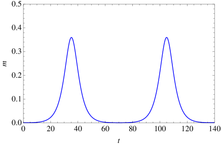
Figure 30: (Color online) The time evolution of $m$ for the interaction ramp $U=0\to 1.25$ in the Hubbard model at half filling with $\beta=40$, $h=10^{-4}$, and $t_{\rm ramp}=10$ obtained from the Hartree approximation.

In Fig. 30, we plot as an example the solution for the interaction ramp $U=0\to 1.25$ given by the Hartree approximation. If the ramp is performed fast enough compared to the development of the order parameter, it can be considered as a quench. The interaction ramp generates an exponential growth of the order parameter, after which it goes through a maximum and returns back to the initial value. The curve of $m(t)$ in Fig. 30 looks like a soliton. In fact, Eq. (93) allows for an analytical soliton solution,

$$m(t)=\frac{2\sqrt{a_{\rm nth}}}{U_{f}\cosh(\sqrt{a_{\rm nth}}t)},$$ (101)

for the initial condition that $m(-\infty)$ is infinitesimal. When the initial value is nonzero, the solution corresponds to a train of solitons as shown in Fig. 30. The period of the soliton train depends on the initial condition and is hence nonuniversal, while the maximum of $m(t)$, $m_{\rm max}=2\sqrt{a_{\rm nth}}/U_{f}$, does not. As we see below, this $m_{\rm max}$ exhibits a universal behavior, which obeys a scaling law different from that for the conventional GL theory.

The nature of the Hartree solution is quite distinct from the DMFT results (Figs. 23 and 27): The Hartree approximation gives a permanently oscillating $m$, whereas the DMFT solution indicates that the amplitude oscillation damps, and $m$ eventually converges to the thermal value $m_{\rm th}$. The difference is apparently coming from the lack of scattering processes in the Hartree approximation. In other words, it is due to the “integrability” of the Hartree equation. However, there seem to exist common universal features in both results. For example, the universality of $m_{\rm max}$ in the Hartree approximation somehow survives even after we take account of correlations in the nonequilibrium DMFT. We examine this point later.

Let us first take a closer look at the coefficient $a_{\rm nth}$ of the quadratic term in $F_{\rm nth}(m)$, since it controls the phase transition. $a_{\rm nth}$ is implicitly determined by Eq. (95), through which $a_{\rm nth}$ can be regarded as a function of $U_{f}$. Assuming that $a_{\rm nth}=a_{\rm nth}(U_{f})$ is a reversible function, we write $U_{f}=U_{f}(a_{\rm nth})$. We now prove that in the vicinity of $a_{\rm nth}=0$, $U_{f}$ varies as

$$U_{f}(a_{\rm nth})=U_{c}^{\rm nth}+c\sqrt{a_{\rm nth}}+O(a_{\rm nth}^{1});$$ (102)

i.e., $U_{f}$ has a square-root dependence on $a_{\rm nth}$ ($c$ is an arbitrary constant). $U_{c}^{\rm nth}\equiv\lim_{a_{\rm nth}\to 0}U_{f}(a_{\rm nth})$ can be interpreted as the critical interaction strength; i.e., the dynamical symmetry breaking is generated when $U_{f}>U_{c}^{\rm nth}$.

To identify $U_{c}^{\rm nth}$, we consider the limit $a_{\rm nth}\to 0$ in Eq. (95). Substituting $a_{\rm nth}=0$ in Eq. (95) gives

$$-U_{c}^{\rm nth}\sum_{\boldsymbol{k}}\frac{f(\epsilon_{\boldsymbol{k}}-\mu_{i}+U_{i}\overline{n})-f(-\epsilon_{\boldsymbol{k}}-\mu_{i}+U_{i}\overline{n})}{2\epsilon_{\boldsymbol{k}}}=1,$$ (103)

which is equivalent to the static mean-field Eq. (79) if we identify $\mu_{i}-U_{i}\overline{n}$ in Eq. (103) with $\mu-U_{c}^{\rm th}\overline{n}$ in Eq. (79) and $U_{c}^{\rm nth}$ in Eq. (103) with $U_{c}^{\rm th}$ in Eq. (79). This identification is allowed if the particle number is conserved (the Hartree approximation is conserving). Hence, the relation $U_{c}^{\rm nth}=U_{c}^{\rm th}\equiv U_{c}$ holds exactly for arbitrary filling within the Hartree approximation.

To see the $a_{\rm nth}$ dependence of $U_{f}$, we take the derivative of Eq. (95) with respect to $a_{\rm nth}$,

$$\frac{dU_{f}^{-1}}{da_{\rm nth}}=\sum_{\boldsymbol{k}}\frac{2\epsilon_{\boldsymbol{k}}}{[(2\epsilon_{\boldsymbol{k}})^{2}+a_{\rm nth}]^{2}}f_{0}(\boldsymbol{k}).$$ (104)

This leads to

$$\frac{dU_{f}}{d\sqrt{a_{\rm nth}}} =-2U_{f}^{2}\sqrt{a_{\rm nth}}\frac{dU_{f}^{-1}}{da_{\rm nth}}$$

$$=-2U_{f}^{2}\int d\epsilon\,D(\epsilon)\frac{(2\epsilon)^{2}\sqrt{a_{\rm nth}}}{[(2\epsilon)^{2}+a_{\rm nth}]^{2}}$$

$$\quad\times\frac{f(\epsilon-\mu_{i}+U_{i}\overline{n})-f(-\epsilon-\mu_{i}+U_{i}\overline{n})}{2\epsilon}.$$ (105)

Let us consider the quantity

$$\frac{(2\epsilon)^{2}\sqrt{a_{\rm nth}}}{[(2\epsilon)^{2}+a_{\rm nth}]^{2}}.$$ (106)

The integral of this quantity does not depend on $a_{\rm nth}$,

$$\int_{-\infty}^{\infty}d\epsilon\,\frac{(2\epsilon)^{2}\sqrt{a_{\rm nth}}}{[(2\epsilon)^{2}+a_{\rm nth}]^{2}} =\int_{-\infty}^{\infty}d\epsilon\,\frac{(2\epsilon)^{2}}{[(2\epsilon)^{2}+1]^{2}}=\frac{\pi}{4},$$ (107)

and

$$\lim_{a_{\rm nth}\to 0}\frac{(2\epsilon)^{2}\sqrt{a_{\rm nth}}}{[(2\epsilon)^{2}+a_{\rm nth}]^{2}}=0\quad(\epsilon\neq 0),$$ (108)

which means

$$\lim_{a_{\rm nth}\to 0}\frac{(2\epsilon)^{2}\sqrt{a_{\rm nth}}}{[(2\epsilon)^{2}+a_{\rm nth}]^{2}} =\frac{\pi}{4}\delta(\epsilon).$$ (109)

By taking the limit $a_{\rm nth}\to 0$ in Eq. (105), we have

$$\lim_{a_{\rm nth}\to 0}\frac{dU_{f}}{d\sqrt{a_{\rm nth}}} =-2U_{c}^{2}\int d\epsilon\,D(\epsilon)\frac{\pi}{4}\delta(\epsilon)$$

$$\quad\times\frac{f(\epsilon-\mu_{i}+U_{i}\overline{n})-f(-\epsilon-\mu_{i}+U_{i}\overline{n})}{2\epsilon}$$

$$=-\frac{\pi}{2}U_{c}^{2}D(0)f^{\prime}(\mu_{i}-U_{i}\overline{n})\equiv c,$$ (110)

which is finite as long as $f^{\prime}(\mu_{i}-U_{i}\overline{n})$ is finite. As a result, one obtains the expansion (102). [Zero temperature is an exception, since $f^{\prime}(\mu_{i}-U_{i}\overline{n})$ diverges or vanishes. At half filling there is a logarithmic correction $U_{f}(a_{\rm nth})\sim-c^{\prime}(\ln a_{\rm nth})^{-1}$, while away from half filling it has a linear dependence $U_{f}(a_{\rm nth})\sim U_{c}+c^{\prime\prime}a_{\rm nth}$ around $a_{\rm nth}=0$.]

The result (102) implies

$$a_{\rm nth}\propto(U_{f}-U_{c})^{2}\quad(U_{f}\geq U_{c}),$$ (111)

which strikingly contrasts with the behavior of the conventional GL free energy $F_{\rm th}(m)$, having $a_{\rm th}\propto(U_{f}-U_{c})^{1}$. The scaling (111) is natural from the point of view of the power counting, since $a_{\rm nth}$ has the dimension of (energy)². Putting $a_{\rm nth}=a_{0}(U_{f}-U_{c})^{2}$ ($a_{0}$ is a dimensionless constant), the nonthermal potential becomes

$$F_{\rm nth}(m)=-\frac{1}{2}a_{0}(U_{f}-U_{c})^{2}m^{2}+\frac{U_{f}^{2}}{8}m^{4}.$$ (112)

The scaling law (111) is “universal”, i.e., the exponent does not depend on details of the problem ($\beta$, $\mu_{i}$, $U_{i}$, $U_{f}$, and other parameters). It defines a new universality class that characterizes the nonequilibrium dynamical symmetry breaking. For example, the maximum of the magnetization curve, $m_{\rm max}$, or the middle point $m_{\rm nth}=(m_{\rm max}+m_{\rm min})/2=m_{\rm max}/2$, scales as

$$m_{\rm nth}\propto m_{\rm max}\propto(U_{f}-U_{c})^{\beta}$$ (113)

with

$$\beta=1.$$ (114)

By comparing this with the thermal scaling (61), we notice that $m_{\rm th}$ becomes much bigger than $m_{\rm nth}$ when $U_{c}^{\rm nth}=U_{c}^{\rm th}$ (which is the case in the Hartree approximation). That is, in the vicinity of the critical point the magnitudes of the thermal and nonthermal order parameters are very different. This leads us to the following scenario. When one goes beyond the Hartree approximation by including correlation effects, $m$ approaches $m_{\rm th}$ in the long-time limit. However, if there exists a “nonthermal critical point,” which may govern the transient order-parameter dynamics, $m$ is trapped for some duration around $m_{\rm nth}$, which can deviate strongly from the final value ($m_{\rm th}$).

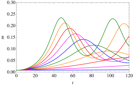
Figure 31: (Color online) Time evolution of $m$ for interaction ramps $U=1.0\to 1.05,1.1,\dots,1.5$ in the Hubbard model at half filling with $\beta=40$, $h=10^{-4}$, and $t_{\rm ramp}=10$.

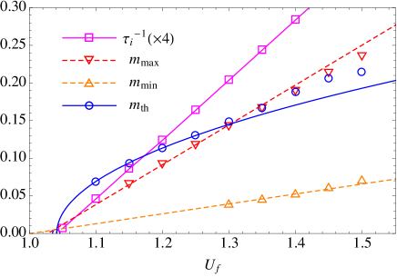
Figure 32: (Color online) The initial exponential growth rate $\tau_{i}$ and the maximum (minimum) value of $m$ at the first peak (dip) of the oscillations for the interaction ramps in Fig. 31.

To confirm the validity of this scenario, we solve a nearly integrable system, i.e., the case with smaller $U_{i}$ and $U_{f}$ than in Fig. 23 or 27, using the nonequilibrium DMFT with the third-order perturbation of type (I) (beyond the Hartree approximation). In Fig. 31, we plot the time evolution of $m$ for interaction ramps $U_{i}=1\to 1.05,1.1,\dots,1.5$. As we decrease $U_{i}$ and $U_{f}$, the magnetization curves approach the form of the Hartree solution (Fig. 30). Due to the presence of the higher-order diagrams, the soliton wave becomes incoherent, and the oscillation center slowly drifts upwards. We measured the time constant of the initial exponential growth, $\tau_{i}$, and the maximum and minimum magnetization, $m_{\rm max}$ and $m_{\rm min}$, at the first peak and dip of the oscillation, which are plotted in Fig. 32. The dashed lines in Fig. 32 are linear extrapolations of $m_{\rm max}$ and $m_{\rm min}$. One can see that both $m_{\rm max}$ and $m_{\rm min}$ linearly approach the critical point, validating the nonthermal scaling (113) and (114) beyond the Hartree approximation. Thus, the transient dynamics of the order parameter is governed by the nonthermal critical point. The extrapolated $m_{\rm max}$ and $m_{\rm min}$ (or the middle point $m_{\rm nth}$) reach zero at $U_{f}=U_{\ast}^{\rm nth}$, which is quite close to the thermal critical point $U_{f}=U_{c}^{\rm th}$ where $\tau_{i}$ diverges. This means that even in calculations which treat correlation effects beyond the Hartree approximation, $U_{\ast}^{\rm nth}$ stays in the close vicinity of $U_{c}^{\rm th}$, at least in the weak-coupling regime.

VII Summary

We have studied the reliability of impurity solvers based on different variants of the weak-coupling perturbation theory in the context of nonequilibrium DMFT, focusing on interaction quenches and ramps in a Hubbard model with semicircular DOS of bandwidth 4. For the PM phase of the Hubbard model at half filling, we have tested the perturbative solvers up to fourth order, and showed that the non-self-consistent fourth-order calculation (bare-diagram expansion of the self-energy) can systematically improve the result of the non-self-consistent second-order expansion (IPT) in the weak-coupling regime ($U<2$), but suddenly fails to conserve the total energy after an interaction quench from $U=0$ to $U>2$. The fourth-order scheme thus fails at approximately the same interaction strength as IPT, which means that going to higher orders in perturbation theory is not a viable strategy for accessing the challenging intermediate coupling regime. While the self-consistent perturbations are conserving, they give a much stronger damping to the thermal state, a behavior which is inconsistent with the result of unbiased QMC calculations.

For the PM phase away from half filling and the AFM phase of the Hubbard model, the perturbation theory has been implemented up to third order. We discussed important details of the weak-coupling expansions, including the choice of bare and bold diagrams, symmetrization of the interaction term, and the treatment of the Hartree diagrams. We considered five types of expansions, as classified in Table 1. Types (III)-(V) lead to a convergence problem in the DMFT self-consistency at moderate and strong interactions, while the type (I) and type (II) schemes always show a nice convergence. Far away from half filling ($|n_{\sigma}-0.5|\geq 0.25$), the third-order expansions of types (I) and (IV) give accurate results, whereas the intermediate filling regime ($0.1<|n_{\sigma}-0.5|<0.25$) remains hard to treat by the perturbation expansions. As one approaches the half-filling regime further, the accuracy improves again. For nonequilibrium dynamics away from half filling, the applicability of the weak-coupling perturbation solvers remains quite limited ($U\leq 1$).

The weak-coupling perturbation theories however turn out to be very useful for the study of the AFM phase near half filling. The third-order expansion of type (I) is the most accurate in the weak $U$ regime ($U<3$), giving reliable results for $T_{c}$ and the staggered magnetization. The second-order perturbation of type (I) reproduces the qualitatively correct weak-to-strong-coupling crossover for $T_{c}$, but it fails to correctly describe the magnetization curve and spectral function in the strong-coupling regime.

We used the nonequilibrium DMFT with the type (I) third-order perturbation theory in an investigation of the dynamical AFM symmetry breaking in the Hubbard model induced by an interaction ramp. The results show that the order parameter starts to grow exponentially, followed by an amplitude oscillation around some nonthermal value, which may be viewed as a “trapping” phenomenon related to the existence of a nonthermal critical point. This amplitude mode is superimposed on top of a slow drift toward the thermal value, and it manifests itself as an oscillating spectral weight transfer in the spectral function.

The phenomenological GL theory cannot consistently explain the dynamics of the order parameter, no matter how the fitting parameter (friction constant) is chosen. We compared the results with the time-dependent Hartree approximation, which allows for analytical soliton solutions. Writing the equation of motion for the order parameter in the form of a GL-like equation, we showed that the nonthermal potential $F_{\rm nth}$ (corresponding to this Hartree solution) belongs to a characteristic universality class (with critical exponent $\beta=1$), which is different from the GL universality ($\beta=\frac{1}{2}$). Due to this fact, the order-parameter dynamics shows a “universality transition” in the critical regime, that is, the order parameter crosses over from the nonthermal value $\propto(U_{f}-U_{c})^{1}$, around which the order parameter is transiently trapped, to the thermal value $\propto(U_{f}-U_{c})^{\frac{1}{2}}$, which is reached in the long-time limit. This qualitative behavior survives to some extent even when $U$ is increased into a regime in which the Hartree approximation breaks down.

There are a couple of issues that are left for future investigations. One is the development of a nonequilibrium impurity solver for calculations away from half filling in the weak-coupling regime, which safely preserves the conservation laws. The bare third-order expansions of types (I) and (IV) seem to be valid in the overdoped regime ($|n_{\sigma}-0.5|>0.25$), while treating the underdoped regime ($0.1<|n_{\sigma}-0.5|<0.25$) remains challenging. The weak-coupling techniques that have been studied in this paper can be applied not only to the AFM phase but also to other symmetry-broken ordered phases such as superconductivity (SC) and CDWs. Indeed, our results of the order-parameter dynamics at half filling can be translated to those for SC and CDW since there is a symmetry between the repulsive and attractive Hubbard models at half filling, via the Shiba transformation (spin-dependent particle-hole exchange).Shiba (1972) Away from half filling, without this symmetry, the dynamics of SC and CDW phases remains to be explored. The interaction quench physics in the SC phase with dilute filling may have direct relevance to cold-atom experiments. A switching from the SC to the CDW phase (or vice versa) would be another interesting topic in connection with related pump-probe experiments.Fausti et al. (2011) The character of the nonthermal critical point that may govern the transient order-parameter dynamics has not been fully revealed. While in this paper we focused on the interaction ramps, an interesting question is if the same universal behavior is observed when we consider other types of perturbations (e.g., a system driven by electric fields). The characterization of the nonthermal critical point (if exists) in the intermediate and strong-coupling regime is also desired and is left as a future problem.

Appendix A Numerical implementation of the nonequilibrium Dyson equation

In this appendix, we describe our numerical implementation of the solution of the nonequilibrium Dyson equation on the Kadanoff-Baym contour $\mathcal{C}$ (Fig. 1). The Dyson equation that one encounters in the nonequilibrium DMFT calculation is an integral-differential equation of the form (12)

$$[i\partial_{t}-\epsilon(t)]G(t,t^{\prime})-\int_{\mathcal{C}}d\overline{t}\,\Sigma(t,\overline{t})G(\overline{t},t^{\prime}) =\delta_{\mathcal{C}}(t,t^{\prime}),$$ (115)

or an integral equation of the form (13)

$$G(t,t^{\prime})-\int_{\mathcal{C}}d\overline{t}\,K(t,\overline{t})G(\overline{t},t^{\prime}) =G_{0}(t,t^{\prime}).$$ (116)

Here $K$, and $G_{0}$ are given contour-ordered functions, and we have to solve these equations for $G$. Let us assume that $\Sigma$ and $K$ do not contain $\delta$ functions. If there is a $\delta$ function inside $\Sigma$ such as a Hartree term, one can include it in $\epsilon(t)$. Using the Langreth rule,Langreth (1976) one can decompose Eq. (115) into the components of the contour functions to rewrite

$$[i\partial_{t}-\epsilon(t)]G^{R}(t,t^{\prime})-\int_{t^{\prime}}^{t}d\overline{t}\,\Sigma^{R}(t,\overline{t})G^{R}(\overline{t},t^{\prime}) =\delta(t,t^{\prime}),$$ (117)

$$[i\partial_{t}-\epsilon(t)]G^{\mbox{$\neg$}}(t,\tau^{\prime})-\int_{0}^{t}d\overline{t}\,\Sigma^{R}(t,\overline{t})G^{\mbox{$\neg$}}(\overline{t},\tau^{\prime}) =Q^{\mbox{$\neg$}}(t,t^{\prime}),$$ (118)

$$[i\partial_{t}-\epsilon(t)]G^{<}(t,t^{\prime})-\int_{0}^{t}d\overline{t}\,\Sigma^{R}(t,\overline{t})G^{<}(\overline{t},t^{\prime}) =Q^{<}(t,t^{\prime}),$$ (119)

where $G^{M}$, $G^{R}$, $G^{\mbox{$\neg$}}$, and $G^{<}$ are the Matsubara, retarded, left-mixing, and lesser components of $G$ (the same notation is applied to other contour functions), respectively, and we have defined

$$Q^{\mbox{$\neg$}}(t,t^{\prime}) =\int_{0}^{\beta}d\overline{\tau}\,\Sigma^{\mbox{$\neg$}}(t,\overline{\tau})G^{M}(\overline{\tau},\tau^{\prime}),$$ (120)

$$Q^{<}(t,t^{\prime}) =\int_{0}^{t^{\prime}}d\overline{t}\,\Sigma^{<}(t,\overline{t})G^{A}(\overline{t},t^{\prime})-i\int_{0}^{\beta}d\overline{\tau}\,K^{\mbox{$\neg$}}(t,\overline{\tau})G^{\reflectbox{$\neg$}}(\overline{t},t^{\prime}).$$ (121)

We can also decompose Eq. (116) into

$$G^{R}(t,t^{\prime})-\int_{t^{\prime}}^{t}d\overline{t}\,K^{R}(t,\overline{t})G^{R}(\overline{t},t^{\prime}) =G_{0}^{R}(t,t^{\prime}),$$ (122)

$$G^{\mbox{$\neg$}}(t,\tau^{\prime})-\int_{0}^{t}d\overline{t}\,K^{R}(t,\overline{t})G^{\mbox{$\neg$}}(\overline{t},\tau^{\prime}) =R^{\mbox{$\neg$}}(t,\tau^{\prime}),$$ (123)

$$G^{<}(t,t^{\prime})-\int_{0}^{t}d\overline{t}\,K^{R}(t,\overline{t})G^{<}(\overline{t},t^{\prime}) =R^{<}(t,t^{\prime}),$$ (124)

where we have defined

$$R^{\mbox{$\neg$}}(t,\tau^{\prime}) =G_{0}^{\mbox{$\neg$}}(t,\tau^{\prime})+\int_{0}^{\beta}d\overline{\tau}\,K^{\mbox{$\neg$}}(t,\overline{\tau})G^{M}(\overline{\tau},\tau^{\prime}),$$ (125)

$$R^{<}(t,t^{\prime}) =G_{0}^{<}(t,t^{\prime})+\int_{0}^{t^{\prime}}d\overline{t}\,K^{<}(t,\overline{t})G^{A}(\overline{t},t^{\prime})$$

$$\quad-i\int_{0}^{\beta}d\overline{\tau}\,K^{\mbox{$\neg$}}(t,\overline{\tau})G^{\reflectbox{$\neg$}}(\overline{\tau},t^{\prime}).$$ (126)

By fixing the second time argument of the contour functions ($t^{\prime}$ or $\tau^{\prime}$), one finds that these equations can be expressed as

$$i\frac{d}{dt}g(t)-\epsilon(t)g(t)-\int_{0}^{t}d\overline{t}\,\Sigma^{R}(t,\overline{t})g(\overline{t})=q(t),$$ (127)

$$g(t)-\int_{0}^{t}d\overline{t}\,K^{R}(t,\overline{t})g(\overline{t})=r(t),$$ (128)

where $g(t)=G(t,\ast)$, $q(t)=Q(t,\ast)$, and $r(t)=R(t,\ast)$. Both of them are categorized as Volterra equations of the second kind, for which various numerical algorithms exist in the literature.Num ; Lin ; Bru Here we present one of them, namely the implicit Runge-Kutta method (or the collocation method), which is employed throughout the paper. For the implementation, we discretize the time with equal spacing, $t_{i}=i\times\Delta t$ ($i=0,1,\dots,N$), with $\Delta t=t_{\rm max}/N$. It is crucial to employ higher-order schemes to accurately simulate the long-time evolution. The $n$th-order scheme has systematic errors of $O(N(\Delta t)^{n+1})=O(t_{\rm max}(\Delta t)^{n})$. Typically we require $n\geq 2$ to control the error. In the following, we present the second-order and fourth-order schemes.

A.1 Second-order scheme

We first treat the Volterra integral-differential equation (127). We set the initial condition, $g(t_{0})=g(0)$, from which we can solve it step by step on the discretized time grid. That is, once $g(t_{i})$ ($i=0,1,\dots,n-1$) and $g^{\prime}(t_{n-1})$ have been obtained, we use these values to determine $g(t_{n})$ and $g^{\prime}(t_{n})$ on the next step. To get $g(t_{n})$, we express the difference between $g(t_{n})$ and $g(t_{n-1})$ by an integral, which is evaluated by the trapezoid integral formula

$$g(t_{n})-g(t_{n-1}) =\int_{t_{n-1}}^{t_{n}}d\overline{t}\,g^{\prime}(\overline{t})\approx\frac{\Delta t}{2}[g^{\prime}(t_{n-1})+g^{\prime}(t_{n})].$$ (129)

Here $g^{\prime}(t_{n-1})$ is already know from the previous calculation, and $g^{\prime}(t_{n})$ is evaluated from Eq. (127),

$$ig^{\prime}(t_{n}) =q(t_{n})+\epsilon(t_{n})g(t_{n})+\int_{0}^{t_{n}}d\overline{t}\,\Sigma^{R}(t_{n},\overline{t})g(\overline{t})$$

$$\approx q(t_{n})+\epsilon(t_{n})g(t_{n})+\Delta t\sum_{i=0}^{n}w_{n,i}\Sigma^{R}(t_{n},t_{i})g(t_{i}),$$ (130)

where we again approximated the integral by the trapezoid rule with weights

$$w_{n,i} =\begin{cases}1/2&i=0,n\\ 1&1\leq n\leq n-1\end{cases}.$$ (131)

Equations (129) and (130) provide a set of linear equations for $g(t_{n})$, which we can solve to obtain

$$g(t_{n}) =\left[1+i\frac{\Delta t}{2}\epsilon(t_{n})+i\frac{(\Delta t)^{2}}{2}w_{n,n}\Sigma^{R}(t_{n},t_{n})\right]^{-1}$$

$$\quad\times\bigg{\{}g(t_{n-1})+\frac{\Delta t}{2}\bigg{[}g^{\prime}(t_{n-1})+q(t_{n})$$

$$\quad-i\Delta t\sum_{i=0}^{n-1}w_{n,i}\Sigma^{R}(t_{n},t_{i})g(t_{i})\bigg{]}\bigg{\}}.$$ (132)

$g^{\prime}(t_{n})$ is derived from Eq. (130) with $g(t_{n})$ substituted by the result (132). The numerical errors are of $O(t_{\rm max}(\Delta t)^{2})$. To avoid repeated calculations of the sums in Eqs. (130) and (132), one should store them in memory.

The same technique can be applied to the Volterra integral equation (128). We evaluate the integral in Eq. (128) by the trapezoid rule and find

$$g(t_{n}) \approx r(t_{n})+\Delta t\sum_{i=0}^{n}w_{n,i}K^{R}(t_{n},t_{i})g(t_{i})$$

$$=\frac{\displaystyle r(t_{n})+\Delta t\sum_{i=0}^{n-1}w_{n,i}K^{R}(t_{n},t_{i})g(t_{i})}{1-\Delta t\,w_{n,n}K^{R}(t_{n},t_{n})}.$$ (133)

It often holds that $K(t_{n},t_{n})=0$, in which case the denominator in Eq. (133) becomes unity.

A.2 Fourth-order scheme

One can derive the fourth-order scheme by replacing the numerical integral formula (trapezoid rule) used in the second-order approximation with higher-order formulas. We need at least three points to evaluate integrals with higher order algorithms. Let us consider the case of $n\geq 2$ first. In this case, we evaluate the difference between $g(t_{n})$ and $g(t_{0})$,

$$g(t_{n})-g(t_{0}) =\int_{t_{0}}^{t_{n}}d\overline{t}\,g^{\prime}(\overline{t})\approx\Delta t\sum_{i=0}^{n}w_{n,i}g^{\prime}(t_{i}),$$ (134)

where one can use Simpson’s rule for $n=2$,

$$w_{2,i} =\begin{cases}1/3&i=0,2,\\ 4/3&i=1,\end{cases}$$ (135)

Simpson’s $3/8$ rule for $n=3$,

$$w_{3,i} =\begin{cases}3/8&i=0,3,\\ 9/8&i=1,2,\end{cases}$$ (136)

the composite Simpson’s rule for $n=4$,

$$w_{4,i} =\begin{cases}1/3&i=0,4,\\ 4/3&i=1,3,\\ 2/3&i=2,\end{cases}$$ (137)

and the fourth-order Gregory’s rule for $n\geq 5$,

$$w_{n,i} =\begin{cases}3/8&i=0,n,\\ 7/6&i=1,n-1,\\ 23/24&i=2,n-2,\\ 1&3\leq i\leq n-3.\end{cases}$$ (138)

$g^{\prime}(t_{n})$ in Eq. (134) is calculated by Eq. (130) with an appropriate higher-order integral formula. In the same way as in the second-order scheme, one arrives at a set of linear equations for $g(t_{n})$, which is solved as

$$g(t_{n}) =\left[1+i\Delta t\,w_{n,n}\epsilon(t_{n})+i(\Delta t\,w_{n,n})^{2}\Sigma^{R}(t_{n},t_{n})\right]^{-1}$$

$$\quad\times\bigg{\{}g(t_{0})+\Delta t\sum_{i=0}^{n-1}w_{n,i}g^{\prime}(t_{i})$$

$$\quad-i\Delta t\,w_{n,n}\bigg{[}q(t_{n})+\Delta t\sum_{i=0}^{n-1}w_{n,i}\Sigma^{R}(t_{n},t_{i})g(t_{i})\bigg{]}\bigg{\}}.$$ (139)

Here one needs $g^{\prime}(t_{i})$ ($0\leq i\leq n-1$), which has to be stored. To avoid that, we employ the relation

$$g(t_{n-1})-g(t_{0})\approx\Delta t\sum_{i=0}^{n-1}w_{n-1,i}g^{\prime}(t_{i}).$$ (140)

With this, we obtain the final expression for the fourth-order scheme,

$$g(t_{n}) =\left[1+i\Delta t\,w_{n,n}\epsilon(t_{n})+i(\Delta t\,w_{n,n})^{2}\Sigma^{R}(t_{n},t_{n})\right]^{-1}$$

$$\quad\times\bigg{\{}g(t_{n-1})+\Delta t\sum_{i=0}^{n-1}(w_{n,i}-w_{n-1,i})g^{\prime}(t_{i})$$

$$\quad-i\Delta t\,w_{n,n}\bigg{[}q(t_{n})+\Delta t\sum_{i=0}^{n-1}w_{n,i}\Sigma^{R}(t_{n},t_{i})g(t_{i})\bigg{]}\bigg{\}}.$$ (141)

Note that $w_{n,i}-w_{n-1,i}=0$ for $0\leq i\leq n-4$ if we use the fourth-order Gregory’s rule (138) for sufficiently large $n$. Hence what one has to store are $g^{\prime}(t_{n-1})$, $g^{\prime}(t_{n-2})$ and $g^{\prime}(t_{n-3})$. The numerical errors are suppressed to $O(N(\Delta t)^{5})=O(t_{\rm max}(\Delta t)^{4})$. For the Volterra integral equation (128), one can use the same expression as in the second-order scheme (133), in combination with the higher-order integral formulas.

The remaining task is to get the starting value $g(t_{1})$. Since the higher-order integral formulas need at least three points on the grid, the above approach cannot be directly applied for $n=1$. One possible solution is to take a very fine grid on the interval $t_{0}\leq t\leq t_{1}$, and use a lower-order integral formula (e.g., trapezoid rule). This approach is simple and straightforward, but the complication is that one has to change the time steps. Another way, which we adopted in the paper, is to take the middle point,Lin $t_{1/2}=\Delta t/2$, and apply Simpson’s rule to the integral from $t_{0}$ to $t_{1}$,

$$g(t_{1})-g(t_{0}) \approx\frac{\Delta t}{6}[g^{\prime}(t_{0})+4g^{\prime}(t_{1/2})+g^{\prime}(t_{1})].$$ (142)

The value at the middle point is obtained from a quadratic interpolation,

$$g^{\prime}(t_{1/2})\approx\frac{3}{8}g^{\prime}(t_{0})+\frac{3}{4}g^{\prime}(t_{1})-\frac{1}{8}g^{\prime}(t_{2}),$$ (143)

which has an error of $O((\Delta t)^{3})$ for the smooth function $g(t)$. Since $g^{\prime}(t_{1/2})$ is multiplied with $\Delta t$ in Eq. (142), the overall error is of $O((\Delta t)^{4})$, which is compatible with the fourth-order scheme. $g^{\prime}(t_{0})$ is known from the initial condition. $g^{\prime}(t_{2})$ is evaluated from Eq. (130) as in the second-order scheme. $g^{\prime}(t_{1})$ is also evaluated from Eq. (130) with Simpson’s rule taking the middle point,

$$ig^{\prime}(t_{1})\approx q(t_{1})+\epsilon(t_{1})G(t_{1})$$

$$+\frac{\Delta t}{6}[\Sigma^{R}(t_{1},t_{0})g(t_{0})+4\Sigma^{R}(t_{1},t_{1/2})g(t_{1/2})+\Sigma^{R}(t_{1},t_{1})g(t_{1})].$$ (144)

One again uses the quadratic interpolation to get the middle-point values,

$$g(t_{1/2}) \approx\frac{3}{8}g(t_{0})+\frac{3}{4}g(t_{1})-\frac{1}{8}g(t_{2}),$$ (145)

$$\Sigma^{R}(t_{1},t_{1/2}) \approx\frac{3}{8}\Sigma^{R}(t_{1},t_{0})+\frac{3}{4}\Sigma^{R}(t_{1},t_{1})+\frac{1}{8}\Sigma^{A}(t_{1},t_{2}).$$ (146)

In Eq. (146), the last term on the right-hand side would be $-\frac{1}{8}\Sigma^{R}(t_{1},t_{2})$ according to the standard interpolation. However, the retarded self-energy $\Sigma^{R}(t,t^{\prime})$ is discontinuous at $t=t^{\prime}$ due to causality, so that the interpolation cannot be applied in this form. Instead of $\Sigma^{R}(t,t^{\prime})$, we can take $\Sigma^{R}(t,t^{\prime})-\Sigma^{A}(t,t^{\prime})=\Sigma^{>}(t,t^{\prime})-\Sigma^{<}(t,t^{\prime})$, which is smooth at $t=t^{\prime}$, and is identical to $\Sigma^{R}(t,t^{\prime})$ for $t\geq t^{\prime}$. Thus, the last term in Eq. (146) should be $+\frac{1}{8}\Sigma^{A}(t_{1},t_{2})$. From Eq. (145), it turns out that to get $g(t_{1})$ we need $g(t_{2})$. On the other hand, $g(t_{2})$ can be determined from $g(t_{0})$ and $g(t_{1})$. In total, we can couple these equations for $g(t_{1})$ and $g(t_{2})$ to determine both simultaneously.

In this way, one can calculate the starting values for every component of $G(t,t^{\prime})$, except for $G^{R}(t_{2},t_{1})$. If we follow the above strategy, $G^{R}(t_{2},t_{1})$ is determined in combination with $G^{R}(t_{3},t_{1})$, which is, however, not available at the first step ($n=2$). As we see below, there is a way to get around this, and $G^{R}(t_{2},t_{1})$ is determined from the knowledge of $G^{R}(t_{1},t_{0})$ and $G^{R}(t_{2},t_{0})$.

We first rewrite the difference between $G^{R}(t_{2},t_{1})$ and $G^{R}(t_{1},t_{1})$ using the trapezoid rule and the middle point $t_{3/2}$,

$$G^{R}(t_{2},t_{1})-G^{R}(t_{1},t_{1})$$

$$\approx\frac{\Delta t}{6}[{G^{R}}^{\prime}(t_{1},t_{1})+4{G^{R}}^{\prime}(t_{3/2},t_{1})+{G^{R}}^{\prime}(t_{2},t_{1})].$$ (147)

Note that the prime indicates the derivative with respect to the first time argument. ${G^{R}}^{\prime}(t_{1},t_{1})$ is given by the initial condition. ${G^{R}}^{\prime}(t_{3/2},t_{1})$ is given by the quadratic interpolation,

$${G^{R}}^{\prime}(t_{3/2},t_{1})\approx\frac{3}{8}{G^{R}}^{\prime}(t_{2},t_{1})+\frac{3}{4}{G^{R}}^{\prime}(t_{1},t_{1})+\frac{1}{8}{G^{A}}^{\prime}(t_{0},t_{1}),$$ (148)

where we have used the fact that ${G^{R}}^{\prime}(t,t^{\prime})-{G^{A}}^{\prime}(t,t^{\prime})={G^{>}}^{\prime}(t,t^{\prime})-{G^{<}}^{\prime}(t,t^{\prime})$ is a smooth function. ${G^{R}}^{\prime}(t_{2},t_{1})$ is determined by Eq. (117); i.e.,

$$i{G^{R}}^{\prime}(t_{2},t_{1}) \approx\epsilon(t_{2})G^{R}(t_{2},t_{1})+\frac{\Delta t}{6}[\Sigma^{R}(t_{2},t_{1})G^{R}(t_{1},t_{1})$$

$$\quad+4\Sigma^{R}(t_{2},t_{3/2})G^{R}(t_{3/2},t_{1})+\Sigma^{R}(t_{2},t_{2})G^{R}(t_{2},t_{1})].$$ (149)

Using appropriate interpolations, we can substitute $\Sigma^{R}(t_{2},t_{3/2})$ and $G^{R}(t_{3/2},t_{1})$ with integer-point values. To evaluate ${G^{A}}^{\prime}(t_{0},t_{1})$ in Eq. (148), we use the conjugate Dyson equation,

$$[i\partial_{t}-\epsilon(t)]G^{A}(t,t^{\prime})-\int_{t}^{t^{\prime}}d\overline{t}\,\Sigma^{A}(t,\overline{t})G^{A}(\overline{t},t^{\prime})=\delta(t,t^{\prime}).$$ (150)

[Note that ${G^{A}}^{\prime}(t,t^{\prime})\neq{G^{R}}^{\prime}(t^{\prime},t)^{\ast}$.] With this, ${G^{A}}^{\prime}(t_{0},t_{1})$ is given by

$$i{G^{A}}^{\prime}(t_{0},t_{1}) \approx\epsilon(t_{0})G^{A}(t_{0},t_{1})+\frac{\Delta t}{6}[\Sigma^{A}(t_{0},t_{0})G^{A}(t_{0},t_{1})$$

$$\quad+4\Sigma^{A}(t_{0},t_{1/2})G^{A}(t_{1/2},t_{1})+\Sigma^{A}(t_{0},t_{1})G^{A}(t_{1},t_{1})].$$ (151)

Again, we employ quadratic interpolations to evaluate $\Sigma^{A}(t_{0},t_{1/2})$ and $G^{A}(t_{1/2},t_{1})$. Thus, we have obtained a set of linear equations to determine $G^{R}(t_{2},t_{1})$ from known functions.

The same technique is applicable to the Volterra integral equation (128) to get the starting values at fourth order. In this case, one has to be particularly careful when one uses a quadratic interpolation like

$$K^{R}(t_{1},t_{1/2})\approx\frac{3}{8}K^{R}(t_{1},t_{0})+\frac{3}{4}K^{R}(t_{1},t_{1})+\frac{1}{8}K^{A}(t_{1},t_{2}).$$ (152)

The contour function $K$ is usually defined as a convolution of two contour functions such as $K=G_{0}\ast\Sigma$, which implies that $K^{A}(t,t^{\prime})\neq K^{R}(t^{\prime},t^{\prime})^{\ast}$. Instead of taking the complex conjugate, one should go back to the original definition of the convolution,

$$K^{A}(t,t^{\prime}) =\int_{t}^{t^{\prime}}d\overline{t}\,\Sigma^{A}(t,\overline{t})G_{0}^{A}(\overline{t},t^{\prime}).$$ (153)

From this, we have

$$K^{A}(t_{1},t_{2}) \approx\frac{\Delta t}{6}[\Sigma^{A}(t_{1},t_{1})G_{0}^{A}(t_{1},t_{2})+4\Sigma^{A}(t_{1},t_{3/2})G^{A}(t_{3/2},t_{2})$$

$$\quad+\Sigma^{A}(t_{1},t_{2})G^{A}(t_{2},t_{2})].$$ (154)

To summarize, we have overviewed the fourth-order implicit Runge-Kutta method for the Volterra integral(-differential) equations. The higher-order scheme is quite important when one tackles the problem of calculating the long-time evolution within nonequilibrium DMFT, keeping the errors down to $O(N(\Delta t)^{5})=O(t_{\rm max}(\Delta t)^{4})$. The subtle issue of computing the starting values in the fourth-order scheme can be overcome with the middle-point approach and quadratic interpolations.

References

- Ogasawara et al. (2000) T. Ogasawara, M. Ashida, N. Motoyama, H. Eisaki, S. Uchida, Y. Tokura, H. Ghosh, A. Shukla, S. Mazumdar, and M. Kuwata-Gonokami, Phys. Rev. Lett. 85, 2204 (2000).
- Iwai et al. (2003) S. Iwai, M. Ono, A. Maeda, H. Matsuzaki, H. Kishida, H. Okamoto, and Y. Tokura, Phys. Rev. Lett. 91, 057401 (2003).
- Perfetti et al. (2006) L. Perfetti, P. A. Loukakos, M. Lisowski, U. Bovensiepen, H. Berger, S. Biermann, P. S. Cornaglia, A. Georges, and M. Wolf, Phys. Rev. Lett. 97, 067402 (2006).
- Okamoto et al. (2007) H. Okamoto, H. Matsuzaki, T. Wakabayashi, Y. Takahashi, and T. Hasegawa, Phys. Rev. Lett. 98, 037401 (2007).
- Wall et al. (2011) S. Wall, D. Brida, S. R. Clark, H. P. Ehrke, D. Jaksch, A. Ardavan, S. Bonora, H. Uemura, Y. Takahashi, T. Hasegawa, et al., Nat. Phys. 7, 114 (2011).
- Bloch et al. (2008) I. Bloch, J. Dalibard, and W. Zwerger, Rev. Mod. Phys. 80, 885 (2008).
- Jördens et al. (2008) R. Jördens, N. Strohmaier, K. Günter, H. Moritz, and T. Esslinger, Nature 455, 204 (2008).
- Schneider et al. (2008) U. Schneider, L. Hackermüller, S. Will, T. Best, I. Bloch, T. A. Costi, R. W. Helmes, D. Rasch, and A. Rosch, Science 322, 1520 (2008).
- Schmitt et al. (2008) F. Schmitt, P. S. Kirchmann, U. Bovensiepen, R. G. Moore, L. Rettig, M. Krenz, J.-H. Chu, N. Ru, L. Perfetti, D. H. Lu, et al., Science 321, 1649 (2008).
- Hellmann et al. (2010) S. Hellmann, M. Beye, C. Sohrt, T. Rohwer, F. Sorgenfrei, H. Redlin, M. Kalläne, M. Marczynski-Bühlow, F. Hennies, M. Bauer, et al., Phys. Rev. Lett. 105, 187401 (2010).
- Petersen et al. (2011) J. C. Petersen, S. Kaiser, N. Dean, A. Simoncig, H. Y. Liu, A. L. Cavalieri, C. Cacho, I. C. E. Turcu, E. Springate, F. Frassetto, et al., Phys. Rev. Lett. 107, 177402 (2011).
- Matsunaga and Shimano (2012) R. Matsunaga and R. Shimano, Phys. Rev. Lett. 109, 187002 (2012).
- Fausti et al. (2011) D. Fausti, R. I. Tobey, N. Dean, S. Kaiser, A. Dienst, M. C. Hoffmann, S. Pyon, T. Takayama, H. Takagi, and A. Cavalleri, Science 331, 189 (2011).
- (14) S. Kaiser, D. Nicoletti, C. R. Hunt, W. Hu, I. Gierz, H. Y. Liu, M. Le Tacon, T. Loew, D. Haug, B. Keimer, and A. Cavalleri, arXiv:1205.4661.
- Demsar et al. (1999) J. Demsar, K. Biljakovi, and D. Mihailovic, Phys. Rev. Lett. 83, 800 (1999).
- Yusupov et al. (2010) R. Yusupov, T. Mertelj, V. V. Kabanov, S. Brazovskii, P. Kusar, J.-H. Chu, I. R. Fisher, and D. Mihailovic, Nat. Phys. 6, 681 (2010).
- Torchinsky et al. (2013) D. H. Torchinsky, F. Mahmood, A. T. Bollinger, I. Božović, and N. Gedik, Nat. Mater. 12, 387 (2013).
- Matsunaga et al. (2013) R. Matsunaga, Y. I. Hamada, K. Makise, Y. Uzawa, H. Terai, Z. Wang, and R. Shimano, Phys. Rev. Lett. 111, 057002 (2013).
- Kibble (1976) T. W. B. Kibble, J. Phys. A 9, 1387 (1976).
- Zurek (1985) W. H. Zurek, Nature (London) 317, 505 (1985).
- Berges et al. (2004) J. Berges, S. Borsányi, and C. Wetterich, Phys. Rev. Lett. 93, 142002 (2004).
- Moeckel and Kehrein (2008) M. Moeckel and S. Kehrein, Phys. Rev. Lett. 100, 175702 (2008).
- Eckstein et al. (2009) M. Eckstein, M. Kollar, and P. Werner, Phys. Rev. Lett. 103, 056403 (2009).
- Berges et al. (2008) J. Berges, A. Rothkopf, and J. Schmidt, Phys. Rev. Lett. 101, 041603 (2008).
- Werner et al. (2012) P. Werner, N. Tsuji, and M. Eckstein, Phys. Rev. B 86, 205101 (2012).
- Tsuji et al. (2013) N. Tsuji, M. Eckstein, and P. Werner, Phys. Rev. Lett. 110, 136404 (2013).
- Hohenberg and Halperin (1977) P. C. Hohenberg and B. I. Halperin, Rev. Mod. Phys. 49, 435 (1977).
- Polkovnikov et al. (2011) A. Polkovnikov, K. Sengupta, A. Silva, and M. Vengalattore, Rev. Mod. Phys. 83, 863 (2011).
- (29) P. Schmidt and H. Monien, arXiv:cond-mat/0202046 (unpublished).
- Freericks et al. (2006) J. K. Freericks, V. M. Turkowski, and V. Zlatić, Phys. Rev. Lett. 97, 266408 (2006).
- (31) H. Aoki, N. Tsuji, M. Eckstein, M. Kollar, T. Oka, and P. Werner, to be published in Rev. Mod. Phys. (arXiv:1310.5329).
- Georges et al. (1996) A. Georges, G. Kotliar, W. Krauth, and M. J. Rozenberg, Rev. Mod. Phys. 68, 13 (1996).
- Metzner and Vollhardt (1989) W. Metzner and D. Vollhardt, Phys. Rev. Lett. 62, 324 (1989).
- Mühlbacher and Rabani (2008) L. Mühlbacher and E. Rabani, Phys. Rev. Lett. 100, 176403 (2008).
- Werner et al. (2009) P. Werner, T. Oka, and A. J. Millis, Phys. Rev. B 79, 035320 (2009).
- Schiró and Fabrizio (2009) M. Schiró and M. Fabrizio, Phys. Rev. B 79, 153302 (2009).
- Gull et al. (2011) E. Gull, A. J. Millis, A. I. Lichtenstein, A. N. Rubtsov, M. Troyer, and P. Werner, Rev. Mod. Phys. 83, 349 (2011).
- Eckstein and Werner (2010) M. Eckstein and P. Werner, Phys. Rev. B 82, 115115 (2010).
- Arrigoni et al. (2013) E. Arrigoni, M. Knap, and W. von der Linden, Phys. Rev. Lett. 110, 086403 (2013).
- (40) C. Gramsch, K. Balzer, M. Eckstein, and M. Kollar, arXiv:1306.6315.
- (41) A. A. Abrikosov, L. P. Gorkov, and I. E. Dzyaloshinski, Methods of Quantum Field Theory in Statistical Physics (Dover, New York, 1975).
- Rammer (2007) J. Rammer, Quantum Field Theory of Non-equilibrium States (Cambridge University Press, Cambridge, 2007).
- Kamenev (2011) A. Kamenev, Field Theory of Non-Equilibrium Systems (Cambridge University Press, Cambridge, UK, 2011).
- (44) K. Yosida and K. Yamada, Prog. Theor. Phys. Suppl. 46, 244 (1970); K. Yamada, Prog. Theor. Phys. 53, 970 (1975); K. Yosida and K. Yamada, ibid. 53, 1286 (1975).
- (45) B. Horvatić and V. Zlatić, Phys. Status Solidi B 99, 251 (1980); V. Zlatić and B. Horvatić, Phys. Rev. B 28, 6904 (1983); V. Zlatić, B. Horvatić, and D. Šokčević, Z. Phys. B 59, 151 (1985).
- Georges and Kotliar (1992) A. Georges and G. Kotliar, Phys. Rev. B 45, 6479 (1992).
- Zhang et al. (1993) X. Y. Zhang, M. J. Rozenberg, and G. Kotliar, Phys. Rev. Lett. 70, 1666 (1993).
- Freericks (1994) J. K. Freericks, Phys. Rev. B 50, 403 (1994).
- Freericks and Jarrell (1994) J. K. Freericks and M. Jarrell, Phys. Rev. B 50, 6939 (1994).
- Gebhard et al. (2003) F. Gebhard, E. Jeckelmann, S. Mahlert, S. Nishimoto, and R. Noack, Eur. Phys. J. B 36, 491 (2003).
- (51) S. Hershfield, J. H. Davies, and J. W. Wilkins, Phys. Rev. Lett. 67, 3720 (1991); Phys. Rev. B 46, 7046 (1992).
- (52) T. Fujii and K. Ueda, Phys. Rev. B 68, 155310 (2003); J. Phys. Soc. Jpn. 74, 127 (2005).
- Eckstein et al. (2010) M. Eckstein, M. Kollar, and P. Werner, Phys. Rev. B 81, 115131 (2010).
- Aron et al. (2012) C. Aron, G. Kotliar, and C. Weber, Phys. Rev. Lett. 108, 086401 (2012).
- Amaricci et al. (2012) A. Amaricci, C. Weber, M. Capone, and G. Kotliar, Phys. Rev. B 86, 085110 (2012).
- Tsuji et al. (2012) N. Tsuji, T. Oka, H. Aoki, and P. Werner, Phys. Rev. B 85, 155124 (2012).
- (57) L. P. Kadanoff and G. Baym, Quantum Statistical Mechanics (W. A. Benjamin, New York, 1962).
- Keldysh (1965) L. V. Keldysh, Zh. Eksp. Teor. Fiz. 47, 1515 (1965), [Sov. Phys. JETP 20, 1018 (1965)].
- (59) W. H. Press, S. A. Teukolsky, W. T. Vetterling, and B. P. Flannery, Numerical Recipes in C, 2nd ed. (Cambridge University Press, Cambridge, 1992).
- (60) P. Linz, Analytical and Numerical Methods for Volterra Equations, (SIAM, Philadelphia, 1985).
- (61) H. Brunner and P. J. van der Houwen, The Numerical Solution of Volterra Equations (North-Holland, Amsterdam, 1986).
- Rubtsov et al. (2005) A. N. Rubtsov, V. V. Savkin, and A. I. Lichtenstein, Phys. Rev. B 72, 035122 (2005).
- Werner et al. (2010) P. Werner, T. Oka, M. Eckstein, and A. J. Millis, Phys. Rev. B 81, 035108 (2010).
- (64) G. D. Mahan, Many-Particle Physics, 3rd ed. (Plenum, New York, 2000).
- Baym and Kadanoff (1961) G. Baym and L. P. Kadanoff, Phys. Rev. 124, 287 (1961).
- Kajueter and Kotliar (1996) H. Kajueter and G. Kotliar, Phys. Rev. Lett. 77, 131 (1996).
- Koga and Werner (2011) A. Koga and P. Werner, Phys. Rev. A 84, 023638 (2011).
- Keller et al. (1999) M. Keller, W. Metzner, and U. Schollwöck, Phys. Rev. B 60, 3499 (1999).
- Keller et al. (2001) M. Keller, W. Metzner, and U. Schollwöck, Phys. Rev. Lett. 86, 4612 (2001).
- Moeckel and Kehrein (2010) M. Moeckel and S. Kehrein, New J. Phys. 12, 055016 (2010).
- Schiró and Fabrizio (2010) M. Schiró and M. Fabrizio, Phys. Rev. Lett. 105, 076401 (2010).
- Schiró and Fabrizio (2011) M. Schiró and M. Fabrizio, Phys. Rev. B 83, 165105 (2011).
- Kollar et al. (2011) M. Kollar, F. A. Wolf, and M. Eckstein, Phys. Rev. B 84, 054304 (2011).
- Hamerla and Uhrig (2013) S. A. Hamerla and G. S. Uhrig, Phys. Rev. B 87, 064304 (2013).
- (75) S. Hamerla and G. Uhrig, arXiv:1307.3438.
- (76) M. Stark and M. Kollar, arXiv:1308.1610.
- Müller-Hartmann (1989) E. Müller-Hartmann, Z. Phys. B: Condens. Matter 76, 211 (1989).
- Werner et al. (2005) F. Werner, O. Parcollet, A. Georges, and S. R. Hassan, Phys. Rev. Lett. 95, 056401 (2005).
- Schmid (1966) A. Schmid, Phys. Kondens. Mater. 5, 302 (1966).
- Abrahams and Tsuneto (1966) E. Abrahams and T. Tsuneto, Phys. Rev. 152, 416 (1966).
- Sá de Melo et al. (1993) C. A. R. Sá de Melo, M. Randeria, and J. R. Engelbrecht, Phys. Rev. Lett. 71, 3202 (1993).
- Barankov et al. (2004) R. A. Barankov, L. S. Levitov, and B. Z. Spivak, Phys. Rev. Lett. 93, 160401 (2004).
- Anderson (1958) P. W. Anderson, Phys. Rev. 112, 1900 (1958).
- Yuzbashyan et al. (2005) E. A. Yuzbashyan, B. L. Altshuler, V. B. Kuznetsov, and V. Z. Enolskii, Phys. Rev. B 72, 220503 (2005).
- Warner and Leggett (2005) G. L. Warner and A. J. Leggett, Phys. Rev. B 71, 134514 (2005).
- Barankov and Levitov (2006) R. A. Barankov and L. S. Levitov, Phys. Rev. Lett. 96, 230403 (2006).
- Yuzbashyan and Dzero (2006) E. A. Yuzbashyan and M. Dzero, Phys. Rev. Lett. 96, 230404 (2006).
- Shiba (1972) H. Shiba, Prog. Theor. Phys. 48, 2171 (1972).
- Langreth (1976) D. C. Langreth, Linear and Nonlinear Electron Transport in Solids (Plenum Press, New York and London, 1976), edited by J. T. Devreese and V. E. van Doren.