Central Limit Theorems for Classical Likelihood Ratio Tests for High-Dimensional Normal Distributions

Abstract

For random samples of size $n$ obtained from $p$-variate normal distributions, we consider the classical likelihood ratio tests (LRT) for their means and covariance matrices in the high-dimensional setting. These test statistics have been extensively studied in multivariate analysis and their limiting distributions under the null hypothesis were proved to be chi-square distributions as $n$ goes to infinity and $p$ remains fixed. In this paper, we consider the high-dimensional case where both $p$ and $n$ go to infinity with $p/n\to y\in(0,1].$ We prove that the likelihood ratio test statistics under this assumption will converge in distribution to normal distributions with explicit means and variances. We perform the simulation study to show that the likelihood ratio tests using our central limit theorems outperform those using the traditional chi-square approximations for analyzing high-dimensional data.

Keywords: Likelihood ratio test, central limit theorem, high-dimensional data, multivariate normal distribution, hypothesis test, covariance matrix, mean vector, multivariate Gamma function.

AMS 2000 Subject Classification: Primary 62H15; secondary 62H10.

1 Introduction

Traditional statistical theory, particularly in multivariate analysis, does not contemplate the demands of high dimensionality in data analysis due to technological limitations and/or motivations. Consequently, tests of hypotheses and many other modeling procedures in many classical textbooks of multivariate analysis such as Anderson (1958), Muirhead (1982), and Eaton (1983) are well developed under the assumption that the dimension of the dataset, denoted by $p$, is considered a fixed small constant or at least negligible compared with the sample size $n$. However, this assumption is no longer true for many modern datasets, because their dimensions can be proportionally large compared with the sample size. For example, the financial data, the consumer data, the modern manufacturing data and the multimedia data all have this feature. More examples of high-dimensional data can be found in Donoho (2000) and Johnstone (2001).

Recently, Bai et al. (2009) develop corrections to the traditional likelihood ratio test (LRT) to make it suitable for testing a high-dimensional normal distribution $N_{p}(\mathbb{\mu},\mathbb{\Sigma})$ with $H_{0}:\ \mathbb{\Sigma}=\mathbb{I}_{p}\ \ \mbox{vs}\ \ H_{a}:\ \mathbb{\Sigma}\neq\mathbb{I}_{p}.$ The test statistic is chosen to be $L_{n}:=\mbox{tr}(\mathbb{S})-\log|\mathbb{S}|-p,$ where $\mathbb{S}$ is the sample covariance matrix from the data. In their derivation, the dimension $p$ is no longer considered a fixed constant, but rather a variable that goes to infinity along with the sample size $n$, and the ratio between $p=p_{n}$ and $n$ converges to a constant $y$, i.e.,

$$\lim_{n\to\infty}\frac{p_{n}}{n}=y\in(0,1).$$ (1.1)

Jiang et al. (2012) further extend Bai’s result to cover the case of $y=1.$

In this paper, we study several other classical likelihood ratio tests for means and covariance matrices of high-dimensional normal distributions. Most of these tests have the asymptotic results for their test statistics derived decades ago under the assumption of a large $n$ but a fixed $p$. Our results supplement these traditional results in providing alternatives to analyze high-dimensional datasets including the critical case $p/n\to 1.$ We will briefly introduce these likelihood ratio tests next. In Section 2, for each LRT described below, we first review the existing literature, then give our central limit theorem (CLT) results when the dimension and the sample size are comparable. We also make graphs and tables on the sizes and powers of these CLTs based on our simulation study to show that, as both $p$ and $n$ are large, the traditional chi-square approximation behaves poorly and our CLTs improve the approximation very much.

• In Section 2.1, for the normal distribution $N_{p}(\mathbb{\mu},\mathbb{\Sigma}),$ we study the sphericity test $H_{0}:\,\mathbb{\Sigma}=\lambda\mathbb{I}_{p}\ \ \mbox{vs}\ \ H_{a}:\,\mathbb{\Sigma}\neq\lambda\mathbb{I}_{p}$ with $\lambda$ unspecified. We derive the central limit theorem for the LRT statistic when $p/n\to y\in(0,1].$ Its proof is given at Section 5.2.

• In Section 2.2, we derive the CLT for the LRT statistic in testing that several components of a vector with distribution $N_{p}(\mu,\mathbb{\Sigma})$ are independent. The proof is presented at Section 5.3.

• In Section 2.3, we consider the LRT with $H_{0}:N_{p}(\mu_{1},\mathbb{\Sigma}_{1})=\cdots=N_{p}(\mu_{k},\mathbb{\Sigma}_{k}),$ that is, several normal distributions are identical. We prove a CLT for the LRT statistic with the assumption $p/n_{i}\to y_{i}\in(0,1]$ where $n_{i}$ is the sample size of a data set from $N_{p}(\mu_{i},\mathbb{\Sigma}_{i})$ for $i=1,2,\cdots,k.$ The proof of the theorem is arranged at Section 5.4.

• In Section 2.4, the test of the equality of the covariance matrices from several normal distributions are studied, that is, $H_{0}:\mathbb{\Sigma}_{1}=\cdots=\mathbb{\Sigma}_{k}.$ The LRT statistic is evaluated under the assumption $p/n_{i}\to y_{i}\in(0,1]$ for $i=1,\cdots,k.$ This generalizes the work of Bai et al. (2009) and Jiang et al. (2012) from $k=2$ to any $k\geq 2.$ The proof of our result is given at Section 5.5.

• In Section 2.5, we investigate LRT with $H_{0}:\mathbb{\mu}=\mathbb{0},\ \mathbb{\Sigma}=\mathbb{I}_{p}$ for the population distribution $N_{p}(\mathbb{\mu},\mathbb{\Sigma}).$ With the dimension $p$ and the sample size $n$ satisfying $p/n\to y\in(0,1],$ we derive the CLT for the LRT statistic. The corresponding theorem is proved at Section 5.6.

• In Section 2.6, we study the test that the population correlation matrix of a normal distribution is equal to an identity matrix, that is, all of the components of a normal vector are independent (but not necessarily identically distributed). This is different from the test in Section 2.2 that several components of a normal vector are independent. The proof is presented at Section 5.7.

• In Sections 3 and 4, we show some simulation results, state our method of the proofs and conclude by offering some open problems.

One can see the value of $y=\lim(p/n)$ or $y_{i}=\lim(p/n_{i})$ introduced above is restricted to the range that $y\leq 1.$ In fact, when $y>1,$ some matrices involved in the LRT statistics do not have a full rank, and consequently their determinants are equal to zero. As a result, the LRT statistics are not defined, or do not exist.

To our knowledge the central limit theorem of the LRT statistics mentioned above in the context of $p/n\to y\in(0,1]$ are new in the literature. Similar research are Bai et al. (2009) and Jiang et al. (2012). The methods of the proofs in the three papers are different: the Random Matrix Theory is used in Bai et al. (2009); the Selberg integral is used in Jiang et al. (2012). Here we obtain the central limit theorems by analyzing the moments of the LRT statistics.

The organization of the rest of the paper is stated as follows. In Section 2, we give the details for each of the six tests described above. A simulation study on the sizes and powers of these tests is presented in Section 3. A discussion is given in Section 4. The theorems appearing in each section are proved in Section 5. An auxiliary result on complex analysis is proved in the Appendix.

2 Main Results

In this section we present the central limit theorems of six classical LRT statistics mentioned in the Introduction. The six central limit theorems are stated in the following six subsections.

2.1 Testing Covariance Matrices of Normal Distributions Proportional to Identity Matrix

For distribution $N_{p}(\mathbb{\mu},\mathbb{\Sigma}),$ we consider the spherical test

$$H_{0}:\,\mathbb{\Sigma}=\lambda\mathbb{I}_{p}\ \ \mbox{vs}\ \ H_{a}:\,\mathbb{\Sigma}\neq\lambda\mathbb{I}_{p}$$ (2.1)

with $\lambda$ unspecified. Let $\mathbb{x}_{1},\cdots,\mathbb{x}_{n}$ be i.i.d. $\mathbb{R}^{p}$-valued random variables with normal distribution $N_{p}(\mathbb{\mu},\mathbb{\Sigma}).$ Recall

$$\bar{\mathbb{x}}=\frac{1}{n}\sum_{i=1}^{n}\mathbb{x}_{i}\ \ \mbox{and}\ \ \mathbb{S}=\frac{1}{n}\sum_{i=1}^{n}(\mathbb{x}_{i}-\bar{\mathbb{x}})(\mathbb{x}_{i}-\bar{\mathbb{x}})^{\prime}.$$ (2.2)

The likelihood ratio test statistic of (2.1) is first derived by Mauchly (1940) as

$$V_{n}=|\mathbb{S}|\cdot\Big{(}\frac{\mbox{tr}(\mathbb{S})}{p}\Big{)}^{-p}.$$ (2.3)

By Theorem 3.1.2 and Corollary 3.2.19 from Muirhead (1982), under $H_{0}$ in (2.1),

$$\frac{n}{\lambda}\cdot\mathbb{S}\ \ \mbox{and}\ \ \mathbb{Z}^{\prime}\mathbb{Z}\ \mbox{have the same distribution}$$ (2.4)

where $\mathbb{Z}:=(z_{ij})_{(n-1)\times p}$ and $z_{ij}$’s are i.i.d. with distribution $N(0,1).$ This says that, with probability one, $\mathbb{S}$ is not of full rank when $p\geq n$, and consequently $|\mathbb{S}|=0.$ This indicates that the likelihood ratio test of (2.1) only exists when $p\leq n-1$. The statistic $V_{n}$ is commonly known as the ellipticity statistic. Gleser (1966) shows that the likelihood ratio test with the rejection region $\{V_{n}\leq c_{\alpha}\}$ (where $c_{\alpha}$ is chosen so that the test has a significance level of $\alpha$) is unbiased. A classical asymptotic result shows that

$$-(n-1)\rho\log V_{n}\ \ \mbox{converges to}\ \ \chi^{2}(f)$$ (2.5)

in distribution as $n\to\infty$ with $p$ fixed, where

$$\rho=1-\frac{2p^{2}+p+2}{6(n-1)p}\ \ \ \mbox{and}\ \ \ f=\frac{1}{2}(p-1)(p+2).$$ (2.6)

This can be seen from, for example, Theorem 8.3.7 from Muirhead (1982), the Slutsky lemma and the fact that $\rho=\rho_{n}\to 1$ as $n\to\infty$ and $p$ is fixed. The quantity $\rho$ is a correction term to improve the convergence rate.

Now we consider the case when both $n$ and $p$ are large. For clarity of taking limit, let $p=p_{n}$, that is, $p$ depends on $n.$

THEOREM 1

Let $n>p+1$ for all $n\geq 3$ and $V_{n}$ be as in (2.3). Assume $\lim_{n\to\infty}p/n=y\in(0,1]$, then, under $H_{0}$ in (2.1), $(\log V_{n}-\mu_{n})/\sigma_{n}$ converges in distribution to $N(0,1)$ as $n\to\infty,$ where

$$\mu_{n}=-p-\big{(}n-p-\frac{3}{2}\big{)}\log(1-\frac{p}{n-1})\ \ \mbox{and}\ \ \ \ \ \ \ \ \$$

$$\sigma_{n}^{2}=-2\Big{[}\frac{p}{n-1}+\log(1-\frac{p}{n-1})\Big{]}.$$

As discussed below (2.4), the LRT exists as $n\geq p+1$, however, we need a slightly stronger condition that $n>p+1$ because of the definition of $\sigma_{n}^{2}.$ Though $\lambda$ in (2.1) is unspecified, the limiting distribution in Theorem 1 is pivotal, that is, it does not depend on $\lambda.$ This is because $\lambda$ is canceled in the expression of $V_{n}$ in (2.3): $|\alpha\mathbb{S}|=\alpha^{p}|\mathbb{S}|$ and $(\mbox{tr}(\alpha\mathbb{S}))^{-p}=\alpha^{-p}\cdot(\mbox{tr}(\mathbb{S}))^{-p}$ for any $\alpha>0.$

Simulation is run on the approximation in (2.5) and the CLT in Theorem 1. The summary is given in Figure 1. It is seen from Figure 1 that the approximation in (2.5) becomes poorer as $p$ becomes larger relative to $n,$ and at the same time the CLT in Theorem 1 becomes more precise. In fact, the chi-square approximation in (2.5) is far from reasonable when $p$ is large: the $\chi^{2}$ curve and the histogram, which are supposed to be matched, separate from each other with the increase of the value of $p.$ See the caption in Figure 1 for more details.

The sizes and powers of the tests by using (2.5) and by Theorem 1 are estimated from our simulation and summarized in Table 1 at Section 3. A further analysis on this results is presented in the same section.

Finally, when $p\geq n$, we know the LRT does not exist as mentioned above. There are some recent works on choosing other statistics to study the spherical test of (2.1), see, for example, Ledoit and Wolf (2002) and Chen, Zhang and Zhong (2010).

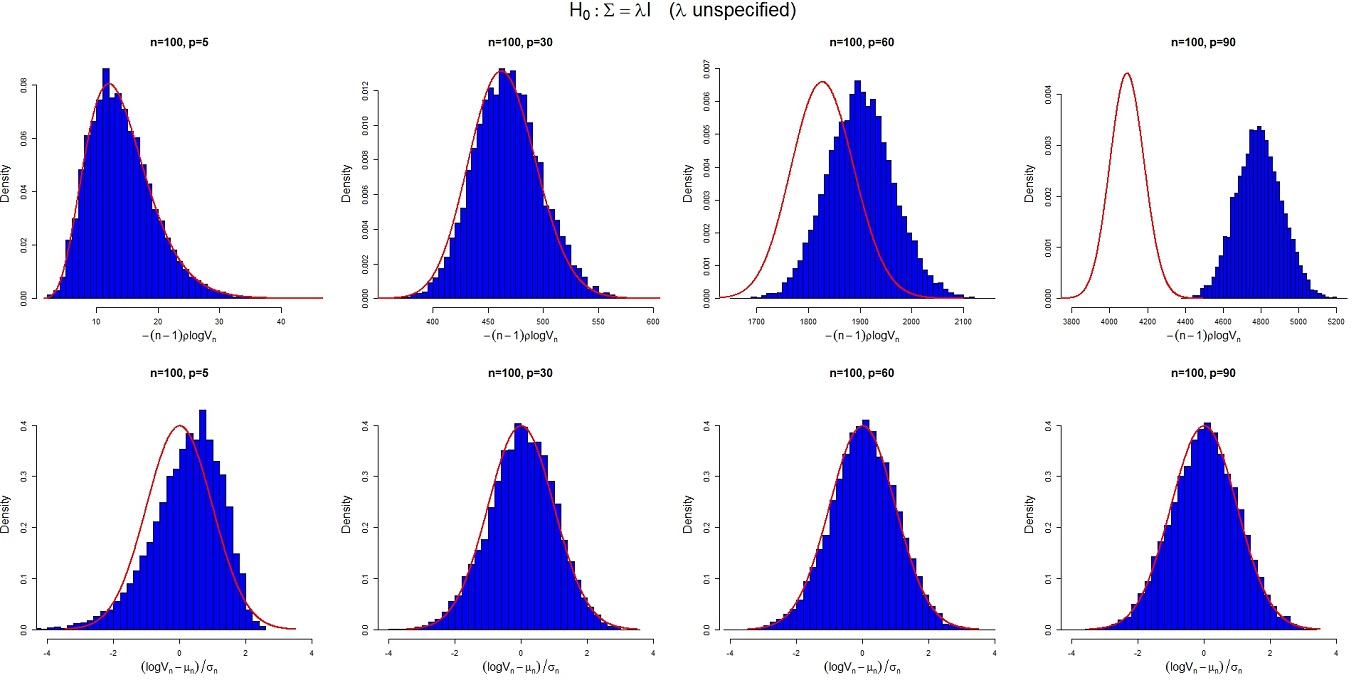
Figure 1: Comparison between Theorem 1 and (2.5). We choose $n=100$ with $p=5,30,60,90.$ The pictures in the top row show that the $\chi^{2}$ curves stay farther away from the histogram of $-(n-1)\rho\log V_{n}$ as $p$ grows. The bottom row shows that the $N(0,1)$-curve fits the histogram of $(\log V_{n}-\mu_{n})/\sigma_{n}$ better as $p$ becomes larger.

2.2 Testing Independence of Components of Normal Distributions

Let $k\geq 2,\,p_{1},\cdots,p_{k}$ be positive integers. Denote $p=p_{1}+\cdots+p_{k}$ and

$$\mathbb{\Sigma}=(\mathbb{\Sigma}_{ij})_{p\times p}$$ (2.7)

be a positive definite matrix, where $\mathbb{\Sigma}_{ij}$ is a $p_{i}\times p_{j}$ sub-matrix for all $1\leq i,j\leq k.$ Let $N_{p}(\mathbb{\mu},\mathbb{\Sigma})$ be a $p$-dimensional normal distribution. We are testing

$$H_{0}:\mathbb{\Sigma}_{ij}=\mathbb{0}\ \mbox{for all}\ 1\leq i<j\leq k\ \ \ \mbox{vs}\ \ \ H_{a}:H_{0}\ \mbox{is not true}.$$ (2.8)

In other words, $H_{0}$ is equivalent to that $\mathbb{\xi}_{1},\cdots,\mathbb{\xi}_{k}$ are independent, where $(\mathbb{\xi}_{1}^{\prime},\cdots,\mathbb{\xi}_{k}^{\prime})^{\prime}$ has the distribution $N_{p}(\mu,\mathbb{\Sigma})$ and $\mathbb{\xi}_{i}\in\mathbb{R}^{p_{i}}$ for $1\leq i\leq k.$ Let $\mathbb{x}_{1},\cdots,\mathbb{x}_{N}$ be i.i.d. with distribution $N_{p}(\mu,\mathbb{\Sigma}).$ Set $n=N-1.$ Let $\mathbb{S}$ be the covariance matrix as in (2.2). Now we partition $\mathbb{A}:=n\mathbb{S}$ in the following way:

$$\mathbb{A}=\left(\begin{array}[]{cccc}\mathbb{A}_{11}&\mathbb{A}_{12}&\cdots&\mathbb{A}_{1k}\\ \mathbb{A}_{21}&\mathbb{A}_{22}&\cdots&\mathbb{A}_{2k}\\ \vdots&\cdots&\cdots&\vdots\\ \mathbb{A}_{k1}&\mathbb{A}_{k2}&\cdots&\mathbb{A}_{kk}\\ \end{array}\right)$$

where $\mathbb{A}_{ij}$ is a $p_{i}\times p_{j}$ matrix. Wilks (1935) shows that the likelihood ratio statistic for testing (2.8) is given by

$$\Lambda_{n}=\frac{|\mathbb{A}|^{(n+1)/2}}{\prod_{i=1}^{k}|\mathbb{A}_{ii}|^{(n+1)/2}}:=(W_{n})^{(n+1)/2},$$ (2.10)

see also Theorem 11.2.1 from Muirhead (1982). Notice that $W_{n}=0$ if $p>N=n+1$, since the matrix $\mathbb{A}$ is not of full rank. From (2.10), we know that the LRT of level $\alpha$ for testing $H_{0}$ in (2.8) is $\{\Lambda_{n}\leq c_{\alpha}\}=\{W_{n}\leq c_{\alpha}^{\prime}\}.$ Set

$$f=\frac{1}{2}\Big{(}p^{2}-\sum_{i=1}^{k}p_{i}^{2}\Big{)}\ \ \mbox{and}\ \ \rho=1-\frac{2\Big{(}p^{3}-\sum_{i=1}^{k}p_{i}^{3}\Big{)}+9\Big{(}p^{2}-\sum_{i=1}^{k}p_{i}^{2}\Big{)}}{6(n+1)\Big{(}p^{2}-\sum_{i=1}^{k}p_{i}^{2}\Big{)}}.$$

When $n$ goes to infinity while all $p_{i}$’s remain fixed, the traditional chi-square approximation to the distribution of $\Lambda_{n}$ is referenced from Theorem 11.2.5 in Muirhead (1982):

$$-2\rho\log\Lambda_{n}\ \mbox{converges to}\ \chi_{f}^{2}\ \mbox{in distribution}$$ (2.11)

as $n\to\infty.$ Now we study the case when $p_{i}$’s are proportional to $n.$ For convenience of taking limit, we assume that $p_{i}$ depends on $n$ for each $1\leq i\leq k.$

THEOREM 2

Assume $n>p+1$ for all $n\geq 3$ and $p_{i}/n\to y_{i}\in(0,1)$ as $n\to\infty$ for each $1\leq i\leq k.$ Recall $W_{n}$ as defined in (2.10). Then, under $H_{0}$ in (2.8), $(\log W_{n}-\mu_{n})/\sigma_{n}$ converges in distribution to $N(0,1)$ as $n\to\infty,$ where

$$\mu_{n}=-r_{n-1}^{2}\Big{(}p-n+\frac{3}{2}\Big{)}+\sum_{i=1}^{k}r_{n-1,i}^{2}\Big{(}p_{i}-n+\frac{3}{2}\Big{)}\ \mbox{and}\ \ \sigma_{n}^{2}=2r_{n-1}^{2}-2\sum_{i=1}^{k}r_{n-1,i}^{2}$$

and $r_{x}=(-\log(1-\frac{p}{x}))^{1/2}$ for $x>p$ and $r_{x,i}=(-\log(1-\frac{p_{i}}{x}))^{1/2}$ for $x>p_{i}$ and $1\leq i\leq k.$

Though $H_{0}$ in (2.8) involves with unknown $\mathbb{\Sigma}_{ii}$’s, the limiting distribution in Theorem 2 is pivotal. This actually can be quickly seen by transforming $\mathbb{y}_{i}=\mathbb{\Sigma}^{-1/2}(\mathbb{x}_{i}-\mu)$ for $1\leq i\leq N.$ Then $\mathbb{y}_{1},\cdots,\mathbb{y}_{N}$ are i.i.d. with distribution $N_{p}(\mathbb{0},\mathbb{I}_{p}).$ Put this into (2.10), the $\mathbb{\Sigma}_{ii}$’s are then canceled in the fraction under the null hypothesis. See also the interpretation in terms of group transformations on p. 532 from Muirhead (1982).

We simulate the two cases in Figure 2: (i) the classical chi-square approximation (2.11); (ii) the central limit theorem based on Theorem 2. The results show that when $p$ becomes large, the classical approximation in (2.11) is poor, however, $(\log W_{n}-\mu_{n})/\sigma_{n}$ in Theorem 2 fits the standard normal curve very well.

In Table 2 from Section 3, we compare the sizes and powers of the two tests under the chosen $H_{a}$ explained in the caption. See the detailed explanations in the same section.

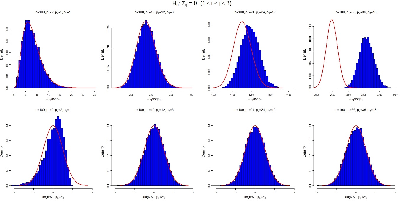
Figure 2: Comparison between Theorem 2 and (2.11). We choose $k=3$, $n=100$ and $p=5,30,60,90$ with $p_{1}:p_{2}:p_{3}=2:2:1$. The pictures in the top row show that the histogram of $-2\rho\log\Lambda_{n}$ move away gradually from $\chi^{2}$ curve as $p$ grows. The pictures in the bottom row indicate that $(\log W_{n}-\mu_{n})/\sigma_{n}$ and $N(0,1)$-curve match better as $p$ becomes larger.

2.3 Testing that Multiple Normal Distributions Are Identical

Given normal distributions $N_{p}(\mu_{i},\mathbb{\Sigma}_{i}),\,i=1,2,\cdots,k,$ we are testing that they are all identical, that is,

$$H_{0}:\mathbb{\mu}_{1}=\cdots=\mathbb{\mu}_{k},\ \mathbb{\Sigma}_{1}=\cdots=\mathbb{\Sigma}_{k}\ \ \mbox{vs}\ H_{a}:H_{0}\ \ \mbox{is not true}.$$ (2.12)

Let $\{\mathbb{y}_{ij};\,1\leq i\leq k,\,1\leq j\leq n_{i}\}$ be independent $p$-dimensional random vectors, and $\{\mathbb{y}_{ij};\,1\leq j\leq n_{i}\}$ be i.i.d. from $N(\mu_{i},\mathbb{\Sigma}_{i})$ for each $i=1,2,\cdots,k.$ Set

$$\mathbb{A}=\sum_{i=1}^{k}n_{i}(\bar{\mathbb{y}}_{i}-\bar{\mathbb{y}})(\bar{\mathbb{y}}_{i}-\bar{\mathbb{y}})^{\prime},\ \ \ \ \ \ \ \ \ \ \mathbb{B}_{i}=\sum_{j=1}^{n_{i}}(\mathbb{y}_{ij}-\bar{\mathbb{y}}_{i})(\mathbb{y}_{ij}-\bar{\mathbb{y}}_{i})^{\prime}\ \ \mbox{and}$$

$$\mathbb{B}=\sum_{i=1}^{k}\mathbb{B}_{i}=\sum_{i=1}^{k}\sum_{j=1}^{n_{i}}(\mathbb{y}_{ij}-\bar{\mathbb{y}}_{i})(\mathbb{y}_{ij}-\bar{\mathbb{y}}_{i})^{\prime}$$

where

$$\bar{\mathbb{y}}_{i}=\frac{1}{n_{i}}\sum_{j=1}^{n_{i}}\mathbb{y}_{ij},\ \ \bar{\mathbb{y}}=\frac{1}{n}\sum_{i=1}^{k}n_{i}\bar{\mathbb{y}}_{i},\ \ n=\sum_{i=1}^{k}n_{i}.$$

The following likelihood ratio test statistic for (2.12) is first derived by Wilks (1932):

$$\Lambda_{n}=\frac{\prod_{i=1}^{k}|\mathbb{B}_{i}|^{n_{i}/2}}{|\mathbb{A}+\mathbb{B}|^{n/2}}\cdot\frac{n^{pn/2}}{\prod_{i=1}^{k}n_{i}^{pn_{i}/2}}.$$ (2.13)

See also Theorem 10.8.1 from Muirhead (1982). The likelihood ratio test will reject the null hypothesis if $\Lambda_{n}\leq c_{\alpha}$, where the critical value $c_{\alpha}$ is determined so that the significance level of the test is equal to $\alpha$. Note that when $p>n_{i}$, the matrix $\mathbb{B}_{i}$ is not of full rank for $i=1,\cdots,k,$ and consequently their determinants are equal to zero, so is the likelihood ratio statistic $\Lambda_{n}$. Therefore, to consider the test of (2.12), one needs $p\leq\min\{n_{i};\,1\leq i\leq k\}.$ Perlman (1980) shows that the LRT is unbiased for testing $H_{0}.$ Let

$$f=\frac{1}{2}p(k-1)(p+3)\ \ \ \mbox{and}\ \ \ \rho=1-\frac{2p^{2}+9p+11}{6(k-1)(p+3)n}\Big{(}\sum_{i=1}^{k}\frac{n}{n_{i}}-1\Big{)}.$$ (2.14)

When the dimension $p$ is considered fixed, the following asymptotic distribution of $\log\Lambda_{n}$ under the null hypothesis (2.12) is a corollary from Theorem 10.8.4 in Muirhead (1982):

$$-2\rho\log\Lambda_{n}\ \ \mbox{converges to}\ \ \chi_{f}^{2}$$ (2.15)

in distribution as $\min_{1\leq i\leq k}{n_{i}}\to\infty.$ When $p$ grows with the same rate of $n_{i}$, we have the following theorem.

THEOREM 3

Let $n_{i}=n_{i}(p)>p+1$ for all $p\geq 1$ and $\lim_{p\to\infty}{p/n_{i}}=y_{i}\in(0,1]$ for all $1\leq i\leq k.$ Let $\Lambda_{n}$ be as in (2.13). Then, under $H_{0}$ in (2.12),

$$\frac{\log\Lambda_{n}-\mu_{n}}{n\sigma_{n}}\ \ \mbox{converges in distribution to}\ N(0,1)$$

as $p\to\infty,$ where

$$\mu_{n}=\frac{1}{4}\Big{[}-2kp-\sum_{i=1}^{k}y_{i}+nr_{n}^{2}(2p-2n+3)-\sum_{i=1}^{k}n_{i}r_{n_{i}^{\prime}}^{2}(2p-2n_{i}+3)\Big{]},$$

$$\sigma_{n}^{2}=\frac{1}{2}\Big{(}\sum_{i=1}^{k}\frac{n_{i}^{2}}{n^{2}}r_{n_{i}^{\prime}}^{2}-r_{n}^{2}\Big{)}>0,$$

$n_{i}^{\prime}=n_{i}-1$ and $r_{x}=\left(-\log\left(1-\frac{p}{x}\right)\right)^{1/2}$ for $x>p.$

The limiting distribution in Theorem 3 is independent of $\mu_{i}$’s and $\mathbb{\Sigma}_{i}$’s. This can be seen by defining $\mathbb{z}_{ij}=\mathbb{\Sigma}_{1}^{-1/2}(\mathbb{y}_{ij}-\mu_{1})$, we then know $\mathbb{z}_{ij}$’s are i.i.d. with distribution $N_{p}(\mathbb{0},\mathbb{I}_{p})$ under the null. It can be easily verified that the $\mu_{i}$’s and $\mathbb{\Sigma}_{i}$’s are canceled from the numerator and the denominator of $\Lambda_{n}$ in (2.13), and hence the right hand side only depends on $\mathbb{z}_{ij}$’s.

From the simulation shown in Figure 3, we see that when $p$ gets larger, the chi-square curve and the histogram are moving farther apart as $p$ becomes large, however, the normal approximation in Theorem 3 becomes better. The sizes and powers are estimated and summarized in Table 3 at Section 3. See more detailed explanations in the same section.

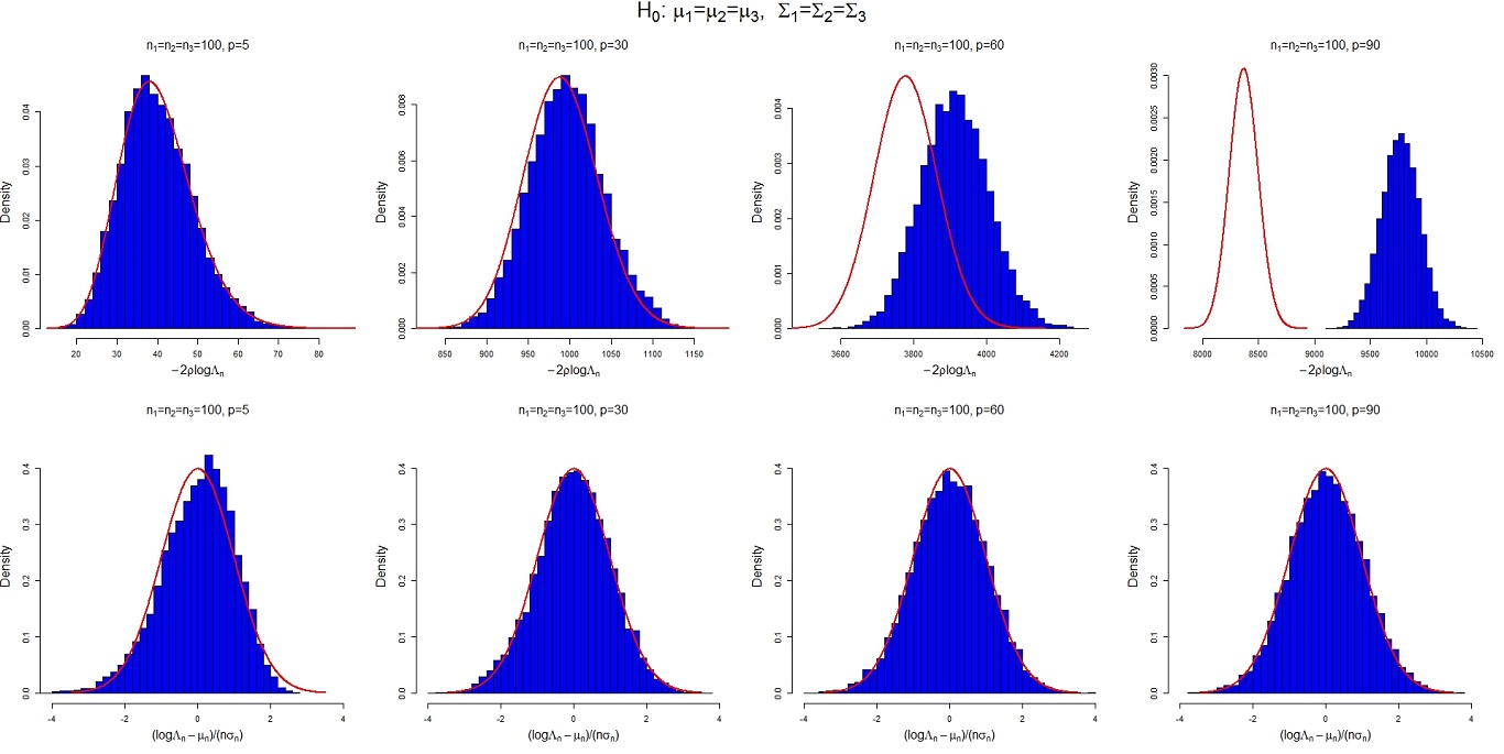
Figure 3: Comparison between Theorem 3 and (2.15). We choose $n_{1}=n_{2}=n_{3}=100$ with $p=5,30,60,90.$ The pictures in the top row show that the $\chi^{2}$ curves stay farther away gradually from the histogram of $-2\rho\log\Lambda_{n}$ as $p$ grows. The pictures in the bottom row show that the $N(0,1)$-curve fits the histogram of $(\log\Lambda_{n}-\mu_{n})/(n\sigma_{n})$ very well as $p$ becomes large.

2.4 Testing Equality of Several Covariance Matrices

Let $k\geq 2$ be an integer. For $1\leq i\leq k,$ let $\mathbb{x}_{i1},\cdots,\mathbb{x}_{in_{i}}$ be i.i.d. $N_{p}(\mathbb{\mu}_{i},\mathbb{\Sigma}_{i})$-distributed random vectors. We are considering

$$H_{0}:\mathbb{\Sigma}_{1}=\cdots=\mathbb{\Sigma}_{k}\ \ \mbox{vs}\ \ \ H_{a}:H_{0}\ \mbox{is not true}.$$ (2.16)

Denote

$$\overline{\mathbb{x}}_{i}=\frac{1}{n_{i}}\sum_{j=1}^{n_{i}}\mathbb{x}_{ij}\ \ \mbox{and}\ \ \ \mathbb{A}_{i}=\sum_{j=1}^{n_{i}}(\mathbb{x}_{ij}-\overline{\mathbb{x}}_{i})(\mathbb{x}_{ij}-\overline{\mathbb{x}}_{i})^{\prime},\ \ \ \ 1\leq i\leq k,$$

and

$$\mathbb{A}=\mathbb{A}_{1}+\cdots+\mathbb{A}_{k}\ \ \ \mbox{and}\ \ \ \ n=n_{1}+\cdots+n_{k}.$$

Wilks (1932) gives the likelihood ratio test of (2.16) with a test statistic

$$\Lambda_{n}=\frac{\prod_{i=1}^{k}\left(\mathrm{det}\mathbf{A}_{i}\right)^{n_{i}/2}}{\left(\mathrm{det}\mathbf{A}\right)^{n/2}}\cdot\frac{n^{np/2}}{\prod_{i=1}^{k}n_{i}^{n_{i}p/2}}$$ (2.17)

and the test rejects the null hypothesis $H_{0}$ at $\Lambda_{n}\leq c_{\alpha}$, where the critical value $c_{\alpha}$ is determined so that the test has the significance level of $\alpha$. Note that $\mathbf{A}_{i}$ does not have a full rank when $p>n_{i}$ for any $i=1,\ldots,k,$ and hence their determinants are equal to zero. So the test statistic $\Lambda_{n}$ is not defined. Therefore, we assume $p\leq n_{i}$ for all $i=1,\ldots,k$ when study the likelihood ratio test of (2.16). The drawback of the likelihood ratio test is on its bias (see Section 8.2.2 of Muirhead (1982)). Bartlett (1937) suggests using a modified likelihood ratio test statistic $\Lambda_{n}^{*}$ by substituting every sample size $n_{i}$ with its degree of freedom $n_{i}-1$ and substituting the total sample size $n$ with $n-k$:

$$\Lambda_{n}^{*}=\frac{\prod_{i=1}^{k}\left(\mathrm{det}\mathbf{A}_{i}\right)^{(n_{i}-1)/2}}{\left(\mathrm{det}\mathbf{A}\right)^{(n-k)/2}}\cdot\frac{(n-k)^{(n-k)p/2}}{\prod_{i=1}^{k}(n_{i}-1)^{(n_{i}-1)p/2}}.$$ (2.18)

The unbiased property of this modified likelihood ratio test is proved by Sugiura and Nagao (1968) for $k=2$ and by Perlman (1980) for a general $k$. Let

$$f=\frac{1}{2}p(p+1)(k-1)\ \ \mbox{and}\ \ \rho=1-\frac{2p^{2}+3p-1}{6(p+1)(k-1)(n-k)}\Big{(}\sum_{i=1}^{k}\frac{n-k}{n_{i}-1}-1\Big{)}.$$

Box (1949) shows that when $p$ remains fixed, under the null hypothesis (2.16),

$$-2\rho\log\Lambda_{n}^{*}\ \ \mbox{converges to}\ \ \chi^{2}_{f}$$ (2.19)

in distribution as $\min_{1\leq i\leq k}n_{i}\to\infty$ (See also Theorem 8.2.7 from Muirhead (1982)). Now, suppose $p$ changes with the sample sizes $n_{i}$’s. We have the following CLT.

THEOREM 4

Assume $n_{i}=n_{i}(p)$ for all $1\leq i\leq k$ such that $\min_{1\leq i\leq k}n_{i}>p+1$ and $\lim_{p\to\infty}p/n_{i}=y_{i}\in(0,1].$ Let $\Lambda_{n}^{*}$ be as in (2.18). Then, under $H_{0}$ in (2.16), $(\log\Lambda_{n}^{*}-\mu_{n})/((n-k)\sigma_{n})$ converges in distribution to $N(0,1)$ as $p\to\infty,$ where

$$\mu_{n}=\frac{1}{4}\Big{[}(n-k)(2n-2p-2k-1)\log(1-\frac{p}{n-k})$$

$$\ \ \ \ \ \ \ \ \ \ \ \ \ \ \ \ \ \ \ \ \ \ \ \ \ \ \ \ \ \ \ \ \ \ -\sum_{i=1}^{k}(n_{i}-1)(2n_{i}-2p-3)\log(1-\frac{p}{n_{i}-1})\Big{]},$$

$$\sigma_{n}^{2}=\frac{1}{2}\Big{[}\log(1-\frac{p}{n-k})-\sum_{i=1}^{k}\Big{(}\frac{n_{i}-1}{n-k}\Big{)}^{2}\log(1-\frac{p}{n_{i}-1})\Big{]}>0.$$

The limiting distribution in Theorem 4 is independent of $\mu_{i}$’s and $\mathbb{\Sigma}_{i}$’s. This is obvious: let $\mathbb{y}_{ij}=\mathbb{\Sigma}_{i}^{-1/2}(\mathbb{x}_{ij}-\mu_{i})$, then $\mathbb{y}_{i}$’s are i.i.d. with distribution $N_{p}(\mathbb{0},\mathbb{I}_{p})$ under the null. From the cancelation of $\mathbb{\Sigma}_{i}$’s in $\Lambda^{*}_{n}$ from (2.18) we see that the distribution of $\Lambda^{*}_{n}$ is free of $\mu_{i}$’s and $\mathbb{\Sigma}_{i}$’s under $H_{0}.$

Bai et al. (2009) and Jiang et al. (2012) study Theorem 4 for the case $k=2.$ Theorem 4 generalizes their results for any $k\geq 2.$ Further, the first four authors impose the condition $\max\{y_{1},y_{2}\}<1$ which excludes the critical case $\max\{y_{1},y_{2}\}=1.$ There is no such a restriction in Theorem 4.

Figure 4 presents our simulation with $k=3.$ It is interesting to see that the chi-square curve and the histogram almost separate from each other when $p$ is large, and at the same time the normal approximation in Theorem 4 becomes very good. In Table 4 from Section 3, we estimate the sizes and powers of the two tests. The analysis is presented in the same section.

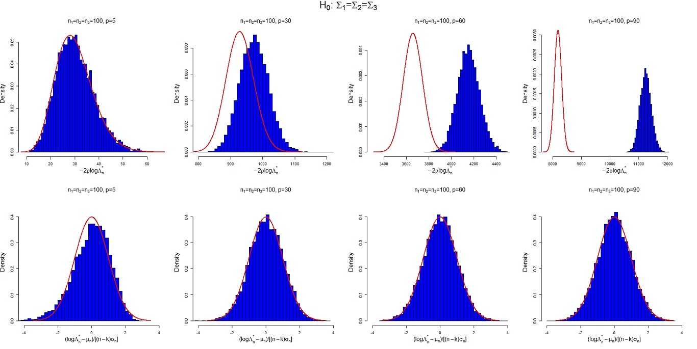
Figure 4: Comparison between Theorem 4 and (2.19). We chose $n_{1}=n_{2}=n_{3}=100$ with $p=5,30,60,90.$ The pictures in the top row show that the $\chi^{2}$ curves goes away quickly from the histogram of $-2\rho\log\Lambda_{n}^{*}$ as $p$ grows. The pictures in the second row show that the $N(0,1)$-curve fits the histogram of $(\log\Lambda^{*}_{n}-\mu_{n})/[(n-k)\sigma_{n}]$ better as $p$ becomes larger.

2.5 Testing Specified Values for Mean Vector and Covariance Matrix

Let $\mathbf{x}_{1},\cdots,\mathbf{x}_{n}$ be i.i.d. $\mathbb{R}^{p}$-valued random vectors from a normal distribution $N_{p}(\mathbf{\mu},\mathbf{\Sigma})$, where $\mathbf{\mu}\in\mathbb{R}^{p}$ is the mean vector and $\mathbf{\Sigma}$ is the $p\times p$ covariance matrix. Consider the hypothesis test:

$$H_{0}: \mathbf{\mu}=\mathbf{\mu}_{0}\ \mathrm{and}\ \mathbf{\Sigma}=\mathbf{\Sigma}_{0}\ \ \mbox{vs}\ \ H_{a}:H_{0}\ \mbox{is not true},$$

where $\mathbf{\mu}_{0}$ is a specified vector in $\mathbb{R}^{p}$ and $\mathbf{\Sigma}_{0}$ is a specified $p\times p$ non-singular matrix. By applying the transformation $\tilde{\mathbf{x}}_{i}=\mathbf{\Sigma}^{-1/2}(\mathbf{x}_{i}-\mathbf{\mu}_{0})$, this hypothesis test is equivalent to the test of:

$$H_{0}: \mathbf{\mu}=\mathbf{0}\ \mathrm{and}\ \mathbf{\Sigma}=\mathbf{I}_{p}\ \ \mbox{vs}\ \ H_{a}:H_{0}\ \mbox{is not true}.$$ (2.20)

Recall the notation

$$\mathbf{\bar{x}}=\frac{1}{n}\sum_{i=1}^{n}\mathbf{x}_{i}\ \ \mbox{and}\ \ \mathbf{A}=\sum_{i=1}^{n}(\mathbf{x}_{i}-\mathbf{\bar{x}})(\mathbf{x}_{i}-\mathbf{\bar{x}})^{\prime}.$$ (2.21)

The likelihood ratio test of size $\alpha$ of (2.20) rejects $H_{0}$ if $\Lambda_{n}\leq c_{\alpha},$ where

$$\Lambda_{n}=\left(\frac{e}{n}\right)^{np/2}|\mathbf{A}|^{n/2}e^{-\mathrm{tr}(\mathbf{A})/2}e^{-n\mathbf{\bar{x}}^{\prime}\mathbf{\bar{x}}/2}.$$ (2.22)

See, for example, Theorem 8.5.1 from Muirhead (1982). Note that the matrix $\mathbf{A}$ does not have a full rank when $p\geq n$ as discussed below (2.4), therefore its determinant is equal to zero. This indicates that the likelihood ratio test of (2.20) only exists when $p<n$. Sugiura and Nagao (1968) and Das Gupta (1969) show that this test with a rejection region $\{\Lambda_{n}\leq c_{\alpha}\}$ is unbiased, where the critical value $c_{\alpha}$ is chosen so that the test has the significance level of $\alpha$.

Theorem 8.5.5 from Muirhead (1982) implies that when the null hypothesis $H_{0}:\mathbf{\mu}=\mathbf{0},\ \mathbf{\Sigma}=\mathbf{I}_{p}$ is true, the statistic

$$-2\rho\log\Lambda_{n}\ \ \mbox{converges to}\ \ \chi^{2}_{f}$$ (2.23)

as $n\to\infty$ with $p$ being fixed, where

$$\rho=1-\frac{2p^{2}+9p+11}{6n(p+3)}\ \ \ \mbox{and}\ \ \ f=\frac{1}{2}p(p+3).$$

Obviously, $\rho=\rho_{n}\to 1$ in this case. Davis (1971) improves the above result with a second order approximation. Nagarsenker and Pillai (1973) study the exact null distribution of $-2\log\Lambda_{n}$ by using its moments. Now we state our CLT result when $p$ grows with $n.$

THEOREM 5

Assume that $p:=p_{n}$ such that $n>1+p$ for all $n\geq 3$ and $\lim_{n\to\infty}p/n=y\in(0,1].$ Let $\Lambda_{n}$ be defined as in (2.22). Then under $H_{0}:\mathbf{\mu}=\mathbf{0}$ and $\mathbf{\Sigma}=\mathbf{I}_{p}$, $(\log\Lambda_{n}-\mu_{n})/(n\sigma_{n})$ converges in distribution to $N(0,1)$ as $n\to\infty$, where

$$\mu_{n}=-\frac{1}{4}\Big{[}n(2n-2p-3)\log(1-\frac{p}{n-1})+2(n+1)p\Big{]}\ \ \mbox{and}\ \ \ \ \ \ \ \ \ \$$

$$\sigma_{n}^{2}=-\frac{1}{2}\Big{(}\frac{p}{n-1}+\log(1-\frac{p}{n-1})\Big{)}>0.$$

The simulations shown in Figure 5 confirm that it is good to use Theorem 5 when $p$ is large and proportional to $n$ rather than the traditional chi-square approximation in (2.23). In Table 5 from Section 3, we study the sizes and powers for the two tests based on the $\chi^{2}$ approximation and our CLT. The understanding of the table is elaborated in the same section.

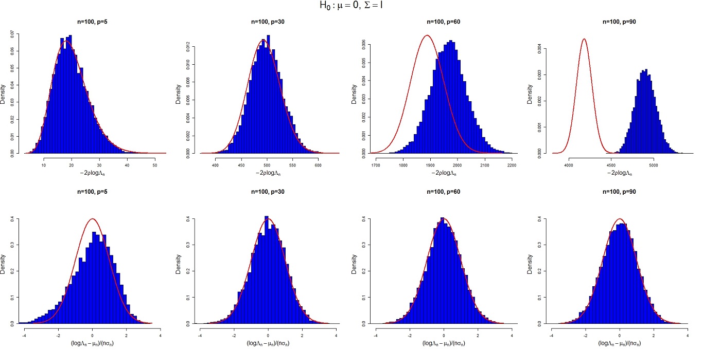
Figure 5: Comparison between Theorem 5 and (2.23). We chose $n=100$ with $p=5,30,60,90.$ The pictures in the top row show that the $\chi^{2}$-curve stays away gradually from the histogram of $-2\log\Lambda_{n}$ as $p$ grows, whereas the $N(0,1)$-curve fits statistic $(\log\Lambda_{n}-\mu_{n})/(n\sigma_{n})$ better as shown from the bottom row.

2.6 Testing Complete Independence

In this section, we study the likelihood ratio test of the complete independence of the coordinates of a high-dimensional normal random vector. Precisely, let $\mathbb{R}=(r_{ij})_{p\times p}$ be the correlation matrix generated from $N_{p}(\mathbb{\mu},\mathbb{\Sigma})$ and $\mathbb{x}=(x_{1},\cdots,x_{p})^{\prime}\sim N_{p}(\mathbb{\mu},\mathbb{\Sigma}).$ The test is

$$H_{0}:\mathbb{R}=\mathbb{I}\ \ \mbox{vs}\ \ H_{a}:\mathbb{R}\neq\mathbb{I}.$$ (2.24)

The null hypothesis $H_{0}$ is equivalent to that $x_{1},\cdots,x_{p}$ are independent or $\mathbb{\Sigma}$ is diagonal. To study the LRT, we need to understand the determinant of a sample correlation matrix generated by normal random vectors. In fact we will have a conclusion on the class of spherical distributions, which is more general than that of the normal distributions. Let us first review two terminologies.

Let $\mathbb{x}=(x_{1},\cdots,x_{n})^{\prime}\in\mathbb{R}^{n}$ and $\mathbb{y}=(y_{1},\cdots,y_{n})^{\prime}\in\mathbb{R}^{n}.$ Recall the Pearson correlation coefficient $r$ defined by

$$r=r_{\mathbb{x},\mathbb{y}}=\frac{\sum_{i=1}^{n}(x_{i}-\bar{\mathbb{x}})(y_{i}-\bar{\mathbb{y}})}{\sqrt{\sum_{i=1}^{n}(x_{i}-\bar{\mathbb{x}})^{2}\cdot\sum_{i=1}^{n}(y_{i}-\bar{\mathbb{y}})^{2}}}$$ (2.25)

where $\bar{\mathbb{x}}=\frac{1}{n}\sum_{i=1}^{n}x_{i}$ and $\bar{\mathbb{y}}=\frac{1}{n}\sum_{i=1}^{n}y_{i}$.

We say a random vector $\mathbb{x}\in\mathbb{R}^{n}$ has a spherical distribution if $\mathbb{O}\mathbb{x}$ and $\mathbb{x}$ have the same probability distribution for all $n\times n$ orthogonal matrix $\mathbb{O}.$ Examples include the multivariate normal distribution $N_{n}(\mathbb{0},\sigma^{2}\mathbb{I}_{n})$, the “$\epsilon$-contaminated” normal distribution $(1-\epsilon)N_{n}(\mathbb{0},\mathbb{I}_{n})+\epsilon N_{n}(\mathbb{0},\sigma^{2}\mathbb{I}_{n})$ with $\sigma>0$ and $\epsilon\in[0,1]$, and the multivariate $t$ distributions. See page 33 from Muirhead (1982) for more discussions.

Let $\mathbb{X}=(x_{ij})_{n\times p}=(\mathbb{x}_{1},\cdots,\mathbb{x}_{n})^{\prime}=(\mathbb{y}_{1},\cdots,\mathbb{y}_{p})$ be an $n\times p$ matrix such that $\mathbb{y}_{1},\cdots,\mathbb{y}_{p}$ are independent random vectors with $n$-variate spherical distributions and $P(\mathbb{y}_{i}=0)=0$ for all $1\leq i\leq p$ (these distributions may be different). Let $r_{ij}=r_{\mathbb{y}_{i},\mathbb{y}_{j}}$, that is, the Pearson correlation coefficient between $\mathbb{y}_{i}$ and $\mathbb{y}_{j}$ for $1\leq i\leq j\leq n.$ Then,

$$\mathbb{R}_{n}:=(r_{ij})_{p\times p}$$ (2.26)

is the sample correlation matrix. It is known that $\mathbb{R}_{n}$ can be written as $\mathbb{R}_{n}=\mathbb{U}^{\prime}\mathbb{U}$ where $\mathbb{U}$ is an $n\times p$ matrix (see, for example, Jiang (2004a)). Thus, $\mathbb{R}_{n}$ does not have a full rank and hence $|\mathbb{R}_{n}|=0$ if $p>n.$ According to Theorem 5.1.3 from Muirhead (1982), the density function of $\mathbb{R}_{n}$ is given by

$$\mbox{Constant}\cdot|\mathbb{R}_{n}|^{(n-p-2)/2}d\,\mathbb{R}_{n}.$$ (2.27)

In the aspect of Random Matrix Theory, the limiting behavior of the largest eigenvalues of $\mathbb{R}_{n}$ and the empirical distributions of the eigenvalues of $\mathbb{R}_{n}$ are investigated by Jiang (2004a). For considering the construction of compressed sensing matrices, the statistical testing problems, the covariance structures of normal distributions, high dimensional regression in statistics and a wide range of applications including signal processing, medical imaging and seismology, the largest off-diagonal entries of $\mathbb{R}_{n}$ are studied by Jiang (2004b), Li and Rosalsky (2006), Zhou (2007), Liu, Lin and Shao (2008), Li, Liu and Rosalsky (2009), Li, Qi and Rolsalski (2010) and Cai and Jiang (2011, 2012).

Let’s now focus on the LRT of (2.24). According to p. 40 from Morrison (2004), the likelihood ratio test will reject the null hypothesis of (2.24) if

$$|\mathbf{R}_{n}|^{n/2}\leq c_{\alpha}$$ (2.28)

where $c_{\alpha}$ is determined so that the test has significant level of $\alpha$. It is also known (see, for example, Bartlett (1954) or p. 40 from Morrison (2005)) that when the dimension $p$ remains fixed and the sample size $n\to\infty$,

$$-\Big{(}n-1-\frac{2p+5}{6}\Big{)}\log|\mathbf{R}_{n}|\overset{d}{\longrightarrow}\chi^{2}_{p(p-1)/2}.$$ (2.29)

This asymptotic result has been used for testing the complete independence of all the coordinates of a normal random vector in the traditional multivariate analysis when $p$ is small relative to $n$.

Now we study the LRT statistic when $p$ and $n$ are large and at the same scale. First, we give a general CLT result on spherical distributions.

THEOREM 6

Let $p=p_{n}$ satisfy $n\geq p+5$ and $\lim_{n\to\infty}p/n=y\in(0,1].$ Let $\mathbb{X}=(\mathbb{y}_{1},\cdots,\mathbb{y}_{p})$ be an $n\times p$ matrix such that $\mathbb{y}_{1},\cdots,\mathbb{y}_{p}$ are independent random vectors with $n$-variate spherical distribution and $P(\mathbb{y}_{i}=\mathbb{0})=0$ for all $1\leq i\leq p$ (these distributions may be different). Recall $\mathbb{R}_{n}$ in (2.26). Then $(\log|\mathbb{R}_{n}|-\mu_{n})/\sigma_{n}$ converges in distribution to $N(0,1)$ as $n\to\infty$, where

$$\mu_{n}=(p-n+\frac{3}{2})\log(1-\frac{p}{n-1})-\frac{n-2}{n-1}p\,;\ \ \ \ \ \ \ \ \ \ \ \ \ \ \ \ \ \$$

$$\sigma_{n}^{2}=-2\Big{[}\frac{p}{n-1}+\log\Big{(}1-\frac{p}{n-1}\Big{)}\Big{]}.$$

In the definition of $\sigma_{n}^{2}$ above, we need the condition $n\geq p+2.$ However, the assumption “$n\geq p+5$” still looks a bit stronger than “$n\geq p+2$”. In fact, we use the stronger one as a technical condition in the proof of Lemma 5.10 which involves the complex analysis.

Notice that when the random vectors $\mathbf{x}_{1},\ldots,\mathbf{x}_{n}$ are i.i.d. from a $p$-variate normal distribution $N_{p}(\mu,\mathbf{\Sigma})$ with complete independence (i.e., $\mathbf{\Sigma}$ is a diagonal matrix or the correlation matrix $\mathbb{R}=\mathbf{I}_{p}$). Write $\mathbb{X}=(x_{ij})_{n\times p}=(\mathbb{x}_{1},\cdots,\mathbb{x}_{n})^{\prime}=(\mathbb{y}_{1},\cdots,\mathbb{y}_{p}).$ Then, $\mathbf{y}_{1},\cdots,\mathbf{y}_{p}$ are independent random vectors from $n$-variate normal distributions (these normal distributions may differ by their covariance matrices). It is also obvious that in this case $P(\mathbf{y}_{i}=0)=0$ for all $1\leq i\leq p$. Therefore, we have the following corollary.

COROLLARY 1

Assume that $p:=p_{n}$ satisfy that $n\geq p+5$ and $\lim_{n\to\infty}p/n=y\in(0,1].$ Let $\mathbf{x}_{1},\cdots,\mathbf{x}_{n}$ be i.i.d. from $N_{p}(\mu,\mathbf{\Sigma})$ with the Pearson sample correlation matrix $\mathbf{R}_{n}$ as defined in (2.26). Then, under $H_{0}$ in (2.24), $(\log|\mathbf{R}_{n}|-\mu_{n})/\sigma_{n}$ converges in distribution to $N(0,1)$ as $n\to\infty$, where

$$\mu_{n}=\Big{(}p-n+\frac{3}{2}\Big{)}\log\left(1-\frac{p}{n-1}\right)-\frac{n-2}{n-1}p;$$

$$\sigma_{n}^{2}=-2\left[\frac{p}{n-1}+\log\left(1-\frac{p}{n-1}\right)\right]>0.$$

According to Corollary 1, the set $\{(\log|\mathbf{R}_{n}|-\mu_{n})/\sigma_{n}\leq-z_{\alpha}\}$ is the rejection region with an asymptotic $1-\alpha$ confidence level for the LRT of (2.24), where the critical value $z_{\alpha}>0$ satisfies that $P(N(0,1)>z_{\alpha})=\alpha$ for all $\alpha\in(0,1).$ Figure 6 shows that the chi-square approximation in (2.29) is good when $p$ is small, but behaves poorly as $p$ is large. At the same time, the normal approximation in Corollary 1 becomes better.

We simulate the sizes and powers of the two tests according to the chi-square approximation in (2.29) and the CLT in Corollary 1 in Table 6 at Section 3. See more analysis in the same section.

As mention earlier, when $p>n$, the LRT statistic $\log|\mathbf{R}_{n}|$ is not defined. So one has to choose other statistics rather than $\log|\mathbf{R}_{n}|$ to study (2.24). See, for example, Schott (2005) and Cai and Ma (2012) for recent progress.

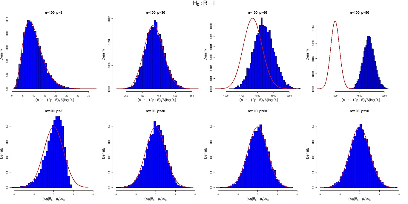
Figure 6: Comparison between Corollary 1 and (2.29). We choose $n=100$ with $p=5,30,60,90.$ The pictures in the first row show that, as $p$ becomes large, the $\chi^{2}$-curve fits the histogram of $-(n-1-\frac{2p+5}{6})\log|\mathbf{R}_{n}|$ poorly. Those in the second row indicate that the N(0,1)-curve fits the histogram of $(\log|\mathbf{R}_{n}|-\mu_{n})/\sigma_{n}$ very well as $p$ becomes large.

3 Simulation Study: Sizes and Powers

In this part, for each of the six LRTs discussed earlier, we run simulation with 10,000 iterations to estimate the sizes and the powers of the LRTs using the CLT approximation and the classical $\chi^{2}$ approximation. An analysis for each table is given. In the following discussion, the notation $\mathbb{J}_{p}$ stands for the $p\times p$ matrix whose entries are all equal to $1$ and $[x]$ stands for the integer part of $x>0.$

(1) Table 1. This table corresponds to the sphericity test that, for $N_{p}(\mathbb{\mu},\mathbb{\Sigma})$, $H_{0}:\,\mathbb{\Sigma}=\lambda\mathbb{I}_{p}\ \ \mbox{vs}\ \ H_{a}:\,\mathbb{\Sigma}\neq\lambda\mathbb{I}_{p}$ with $\lambda$ unspecified. It is studied in Section 2.1. As expected, the $\chi^{2}$ approximation is good when $p$ is small relative to $n$, but not when $p$ is large. For example, at $n=100$ and $p=60,$ the size (type I error or alpha error) for our normal approximation is $0.0511$ and power is $0.7914$, but the size for $\chi^{2}$ approximation is $0.3184$, which is too large to be used in practice. It is very interesting to see that our normal approximation is also as good as the $\chi^{2}$ approximation even when $p$ is small. Moreover, for $n=100$ and $p=90$ where the ratio $y=0.9$ is close to $1$, the type I error in the CLT case is close to $5\%$ and the power is still decent at $0.5406.$ Further, the power for the case of CLT drops as the ratio $p/n$ increases to $1$. This makes sense because the convergence rate of the CLT becomes slow. This can be seen from Theorem 1 that $\sigma_{n}\to\infty$ as $p/n\to 1.$

(2) Table 2. In this table, we compare the sizes and powers of two tests under the chosen $H_{a}$ explained in the caption. The first one is the classical $\chi^{2}$-approximation in (2.11) and the second is the CLT in Theorem 2 for the hypothesis that some components of a normal distribution are independent. We observe from the chart that our CLT approximation and the classical $\chi^{2}$ approximation are comparable for the small values of $p_{i}$’s. However, when $p_{i}$’s are large, noticing the last two rows in the table, our test is good whereas the $\chi^{2}$ approximation is no longer applicable because of the large sizes (type I errors). The power for the CLT drops when the values of $p_{i}$’s become large. This follows from Theorem 2 that $\sigma_{n}\to\infty$ as $\sum p_{i}/n\to 1$, and hence the CLT-approximation does not perform well.

(3) Table 3. We create this table for testing that several normal distributions are identical in Section 2.3. It is easily seen that our CLT is good in all cases (except at the case of $p=5$ where the type I error in our test is $0.0621$, slightly higher than $0.0512$ in the classical case). But when $p=60$ and $n_{1}=n_{2}=n_{3}=100$, the size in the classical case is $0.4542,$ too large to be used. It is worthwhile to notice that the power on the CLT becomes smaller as the value of $p$ becomes larger. This is easily understood from Theorem 3 that the standard deviation diverges to infinity when $p/n\to 1.$ Equivalently, the convergence rate is poorer when $p$ gets closer to $n.$

(4) Table 4. This table relates to the test of the equality of the covariance matrices from $k$ normal distributions studied in Section 2.4. We take $k=3$ in our simulations. The sizes and powers of the chi-square approximation and the CLT in Theorem 4 are summarized in the table. When $p=5$ and $n_{1}=n_{2}=n_{3}=100$, our CLT approximation gives a reasonable size of the test while the classical $\chi^{2}$ approximation is a bit better. However, for the same values of $n_{i}$’s, when $p=30,60,90,$ the size for the $\chi^{2}$ approximation is $0.2607,0.9998$ and $1$, respectively, which are not recommended to be used in practice. Similar to the previous tests, $\sigma_{n}\to\infty$ as $p/n\to 1$, where $\sigma_{n}^{2}$ is as in Theorem 4. This implies that the convergence of the CLT is slow in this case. So it is not surprised to see that the power of the test based on the CLT in the table reduces as $p/n\to 1$.

(5) Table 5. We generate this table by considering the LRT with $H_{0}:\mathbb{\mu}=\mathbb{0},\ \mathbb{\Sigma}=\mathbb{I}_{p}$ for the population distribution $N_{p}(\mathbb{\mu},\mathbb{\Sigma}).$ The CLT is developed in Theorem 5. In this table we study the sizes and powers for the two cases based on the $\chi^{2}$ approximation and the CLT. At $n=100,p=5$ ($p$ is small), the $\chi^{2}$ test outperforms ours. The two cases are equally good at $n=100,p=30.$ When the values of $p$ are large at $60$ and $90,$ our CLT is still good but the $\chi^{2}$ approximation is no longer useful. At the same time, it is easy to spot from the fourth column of the table that the power for the CLT-test drops as the ratio $p/n$ becomes large. It is obvious from Theorem 5 that the standard deviation $\sigma_{n}$ goes to infinity as the ratio approaches one. This causes the less precision when the sample size is not large.

(6) Table 6. This chart is created on the test that all of the components of a normal vector are independent (but not necessarily identically distributed). It is studied in Corollary 1. The sizes and powers of the two tests are estimated from simulation using the chi-square approximation in (2.29) and the CLT in Corollary 1 from Section 3 (the $H_{a}$ is explained in the caption). At all of the four cases of $n=100$ with $p=5,30,60$ and $90,$ the performance of our CLT-test is good, and it is even comparable with the classical $\chi^{2}$-test at the small value of $p=5.$ When $p=60$ and $90,$ the sizes of the $\chi^{2}$-test are too big, while those of the CLT-test keep around $0.05.$ For the CLT-test itself, looking at the third and fourth rows of the table, though the performance corresponding to $y=p/n=0.6$ is better than that corresponding to the high value of $y=p/n=0.9$ as expected, they are quite close. The only difference is the declining of the power as the rate $p/n$ increases. Again, this is easily seen from Corollary 1 that the standard deviation $\sigma_{n}$ is divergent as $p$ is close to $n.$

Table 1: Size and Power of LRT for Sphericity in Section 2.1

	Size under $H_{0}$		Power under $H_{a}$
	CLT	$\chi^{2}$ approx.	CLT	$\chi^{2}$ approx.
$n=100,p=5$	0.0562	0.0491	0.7525	0.7317
$n=100,p=30$	0.0581	0.0686	0.8700	0.8867
$n=100,p=60$	0.0511	0.3184	0.7914	0.9759
$n=100,p=90$	0.0518	1.0000	0.5406	1.0000

The sizes (alpha errors) are estimated based on $10,000$ simulations from $N_{p}(\mathbf{0},\mathbf{I}_{p})$. The powers are estimated under the alternative hypothesis that $\mathbf{\Sigma}=diag(1.69,\cdots,1.69,1,\cdots,1)$, where the number of 1.69 on the diagonal is equal to $[p/2]$.

Table 2: Size and Power of LRT for Independence of Three Components in Section 2.2

	Size under $H_{0}$		Power under $H_{a}$
	CLT	$\chi^{2}$ approx.	CLT	$\chi^{2}$ approx.
$n=100,p_{1}=2,p_{2}=2,p_{3}=1$	0.0647	0.0458	0.7605	0.7176
$n=100,p_{1}=12,p_{2}=12,p_{3}=6$	0.0518	0.0543	0.9768	0.9778
$n=100,p_{1}=24,p_{2}=24,p_{3}=12$	0.0496	0.2171	0.8651	0.9757
$n=100,p_{1}=36,p_{2}=36,p_{3}=18$	0.0537	0.9998	0.4850	1.0000

The sizes (alpha errors) are estimated based on $10,000$ simulations from $N_{p}(\mathbf{0},\mathbf{I}_{p})$. The powers are estimated under the alternative hypothesis that $\mathbf{\Sigma}=0.15\mathbf{J}_{p}+0.85\mathbf{I}_{p}$.

Table 3: Size and Power of LRT for Equality of Three Distributions in Section 2.3

	Size under $H_{0}$		Power under $H_{a}$
	CLT	$\chi^{2}$ approx.	CLT	$\chi^{2}$ approx.
$n_{1}=n_{2}=n_{3}=100,p=5$	0.0621	0.0512	0.7420	0.7135
$n_{1}=n_{2}=n_{3}=100,p=30$	0.0588	0.0743	0.8727	0.8936
$n_{1}=n_{2}=n_{3}=100,p=60$	0.0531	0.4542	0.6864	0.9770
$n_{1}=n_{2}=n_{3}=100,p=90$	0.0488	1.0000	0.3493	1.0000

The sizes (alpha errors) are estimated based on $10,000$ simulations from three normal distributions of $N_{p}(\mathbf{0},\mathbf{I}_{p})$. The powers were estimated under the alternative hypothesis that $\mathbf{\mu}_{1}=(0,\ldots,0)^{\prime}$, $\mathbf{\Sigma}_{1}=0.5\mathbf{J}_{p}+0.5\mathbf{I}_{p}$; $\mathbf{\mu}_{2}=(0.1,\ldots,0.1)^{\prime}$, $\mathbf{\Sigma}_{2}=0.6\mathbf{J}_{p}+0.4\mathbf{I}_{p}$; $\mathbf{\mu}_{3}=(0.1,\ldots,0.1)^{\prime}$, $\mathbf{\Sigma}_{3}=0.5\mathbf{J}_{p}+0.31\mathbf{I}_{p}$.

Table 4: Size and Power of LRT for Equality of Three Covariance Matrices in Section 2.4

	Size under $H_{0}$		Power under $H_{a}$
	CLT	$\chi^{2}$ approx.	CLT	$\chi^{2}$ approx.
$n_{1}=n_{2}=n_{3}=100,p=5$	0.0805	0.0567	0.7157	0.6586
$n_{1}=n_{2}=n_{3}=100,p=30$	0.0516	0.2607	0.6789	0.9218
$n_{1}=n_{2}=n_{3}=100,p=60$	0.0525	0.9998	0.4493	1.0000
$n_{1}=n_{2}=n_{3}=100,p=90$	0.0535	1.0000	0.2297	1.0000

The sizes (alpha errors) are estimated based on $10,000$ simulations from $N_{p}(\mathbf{0},\mathbf{I}_{p})$. The powers are estimated under the alternative hypothesis that $\mathbf{\Sigma}_{1}=\mathbf{I}_{p}$, $\mathbf{\Sigma}_{2}=1.1\mathbf{I}_{p}$, and $\mathbf{\Sigma}_{3}=0.9\mathbf{I}_{p}$.

Table 5: Size and Power of LRT for Specified Normal Distribution in Section 2.5

	Size under $H_{0}$		Power under $H_{a}$
	CLT	$\chi^{2}$ approx.	CLT	$\chi^{2}$ approx.
$n=100,p=5$	0.0986	0.0471	0.5106	0.3818
$n=100,p=30$	0.0611	0.0657	0.7839	0.7898
$n=100,p=60$	0.0584	0.3423	0.7150	0.9583
$n=100,p=90$	0.0571	1.0000	0.4752	1.0000

Sizes (alpha errors) are estimated based on $10,000$ simulations from $N_{p}(\mathbf{0},\mathbf{I}_{p})$. The powers are estimated under the alternative hypothesis that $\mathbf{\mu}=(0.1,\ldots,0.1,0,\ldots,0)^{\prime}$ where the number of $0.1$ is equal to $[p/2]$ and $\mathbf{\Sigma}=\{\sigma_{ij}\}$ where $\sigma_{ij}=1$ for $i=j$, $\sigma_{ij}=0.1$ for $0<|i-j|\leq 3$, and $\sigma_{ij}=0$ for $|i-j|>3$.

Table 6: Size and Power of LRT for Complete Independence in Section 2.6

	Size under $H_{0}$		Power under $H_{a}$
	CLT	$\chi^{2}$ approx.	CLT	$\chi^{2}$ approx.
$n=100,p=5$	0.0548	0.0520	0.4311	0.4236
$n=100,p=30$	0.0526	0.0606	0.6658	0.6945
$n=100,p=60$	0.0522	0.3148	0.5828	0.9130
$n=100,p=90$	0.0560	1.0000	0.3811	1.0000

Sizes (alpha errors) are estimated based on $10,000$ simulations from $N_{p}(\mathbf{0},\mathbf{I}_{p})$. The powers are estimated under the alternative hypothesis that the correlation matrix $\mathbf{R}=(r_{ij})$ where $r_{ij}=1$ for $i=j$, $r_{ij}=0.1$ for $0<|i-j|\leq 3$, and $r_{ij}=0$ for $|i-j|>3$.

4 Conclusions and Discussions

In this paper, we consider the likelihood ratio tests for the mean vectors and covariance matrices of high-dimensional normal distributions. Traditionally, these tests were performed by using the chi-square approximation. However, this approximation relies on a theoretical assumption that the sample size $n$ goes to infinity, while the dimension $p$ remains fixed. As many modern datasets discussed in Section 1 feature high dimensions, these traditional likelihood ratio tests were shown to be less accurate in analyzing those datasets.

Motivated by the pioneer work of Bai et al. (2009) and Jiang et al. (2012), who prove two central limit theorems of the likelihood ratio test statistics for testing the high-dimensional covariance matrices of normal distributions, we examine in this paper other LRTs that are widely used in the multivariate analysis and prove the central limit theorems for their test statistics. By using the method developed in Jiang et al. (2012), that is, the asymptotic expansion of the multivariate Gamma function with high dimension $p$, we are able to derive the central limit theorems without relying on concrete random matrix models as demonstrated in Bai et al. (2009). Our method also has an advantage that the central limit theorems for the critical cases $\lim(p/n)=y=1$ or $\lim(p/n_{i})=y_{i}=1$ are all derived, which is not the case in Bai et al. (2009) because of the restriction of their tools from the Random Matrix Theory. In real data analysis, as long as $n>p+1$ or $n_{i}>p+1$ in Theorems 1-5, or $n\geq p+5$ in Theorem 6, we simply take $y=p/n$ or $y_{i}=p/n_{i}$ to use the theorems. As Figures 1-6 and Tables 1-6 show, our CLT-approximations are all good even though $p$ is relatively small.

The proofs in this paper are based on the analysis of the moments of the LRT statistics (five of six such moments are from literature and the last one is derived by us as in Lemma 5.10). The moment method we use here is different from that of the Random Matrix Theory employed in Bai et al. (2009) and the Selberg integral used in Jiang et al. (2012).

Our research also brings out the following four interesting open problems:

1. All our central limit theorems in this paper are proved under the null hypothesis. As people want to assess the power of the test in many cases, it is also interesting to study the distribution of the test statistic under an alternative hypothesis. In the traditional case where $p$ is considered to be fixed while $n$ goes to infinity, the asymptotic distributions of many likelihood ratio statistics under the alternative hypotheses are derived by using the zonal polynomials (see, e.g., Section 8.2.6, Section 8.3.4, Section 8.4.5 from Muirhead (1982)). It can be conjectured that in the high-dimensional case, there could be some new results regarding the limiting distributions of the test statistics under the alternative hypotheses. However, this is non-trivial and may require more investigation of the high-dimensional zonal polynomials. Some new understanding about the connection between the random matrix theory and the Jack polynomials (the zonal polynomials, the Schur polynomials and the zonal spherical functions are special cases) is given by Jiang and Matsumoto (2011). A recent work by Bai et al. (2009) study the high-dimensional LRTs through the random matrix theory. So the connection among the random matrix theory, LRTs and the Jack polynomials is obvious. We are almost sure that the understanding by Jiang and Matsumoto (2011) will be useful in exploring the LRT statistics under the alternative hypotheses.

2. Except Theorem 6 where the condition $n\geq p+5$ is imposed due to a technical constraint, all other five central limit theorems in this paper are proved under the condition $n>p+1$ or $n_{i}>p+1$. This is because when this is not the case in the five theorems, the likelihood ratio statistics will become undefined in these five cases. This indicates that tests other than the likelihood ratio ones shall be developed for analyzing a dataset with $p$ greater than $n$. For recent progress, see, for example, Ledoit and Wolf (2002) and Chen et al. (2010) for the sphericity test, and Schott (2001, 2007) for testing the equality of multiple covariance matrices and Srivastava (2005) for testing the covariance matrix of a normal distribution. A power study for sphericity test is tried by Onatski et al. Despite these enlightening work mentioned above, other hypothesis tests for $p>n$ or $p>n_{i}$ are still an open area with many interesting problems to be solved.

3. In this paper we consider the cases when $p$ and $n$ or $n_{i}$ are proportional to each other, that is, $\lim p/n=y\in(0,1]$ or $\lim p/n_{i}=y_{i}\in(0,1].$ In practice, $p$ may be large but may not be large enough to be at the same scale of $n$ or $n_{i}$. So it is useful to derive the central limit theorems appeared in this paper under the assumption that $p\to\infty$ such that $p/n\to 0$ or $p/n_{i}\to 0$.

4. To understand the robustness of the six likelihood tests in this paper, one has to study the limiting behaviors of the LRT statistics without the normality assumptions. This is feasible. For example, in Section 2.2 we test the independence of several components of a normal distribution. The LRT statistic $W_{n}$ in (2.10) can be written as the product of some independent random variables, say, $V_{i}$’s with beta distributions (see, e.g., Theorem 11.2.4 from Muirhead (1982)). Therefore, it is possible that we can derive the CLT of $W_{n}$ for general $V_{i}$’s with the same means and variances as those of the beta distributions.

Finally, it is worthwhile to mention that some recent works consider similar problems under the nonparametric setting, see, e.g., Cai et al. (2013), Cai and Ma, Chen et al. (2010), Li and Chen (2012), Qiu and Chen (2012) and Xiao and Wu (2013).

5 Proofs

This section is divided into some subsections. In each of them we prove a theorem introduced in Section 1. We first develop some tools. The following are some standard notation.

For two sequence of numbers $\{a_{n};\,n\geq 1\}$ and $\{b_{n};\,n\geq 1\}$, the notation $a_{n}=O(b_{n})$ as $n\to\infty$ means that $\limsup_{n\to\infty}|a_{n}/b_{n}|<\infty.$ The notation $a_{n}=o(b_{n})$ as $n\to\infty$ means that $\lim_{n\to\infty}a_{n}/b_{n}=0.$ For two functions $f(x)$ and $g(x)$, the notation $f(x)=O(g(x))$ and $f(x)=o(g(x))$ as $x\to x_{0}\in[-\infty,\infty]$ are similarly interpreted.

Throughout the paper $\Gamma(z)$ is the Gamma function defined on the complex plane $\mathbb{C}.$

5.1 A Preparation

LEMMA 5.1

Let $b:=b(x)$ be a real-valued function defined on $(0,\infty)$. Then,

$$\log\frac{\Gamma(x+b)}{\Gamma(x)}=b\log x+\frac{b^{2}-b}{2x}+c(x)$$

as $x\to+\infty$, where

$$c(x)=\begin{cases}O(x^{-1/2}),&\text{if\, $b(x)=O(\sqrt{x}\,)$;}\\ O(x^{-2}),&\text{if\, $b(x)=O(1).$}\end{cases}$$

Further, for any constants $d>c,$ as $x\to+\infty$,

$$\sup_{c\leq t\leq d}\Big{|}\log\frac{\Gamma(x+t)}{\Gamma(x)}-t\log x\Big{|}\to 0.$$

Proof. Recall the Stirling formula (see, e.g., p. 368 from Gamelin (2001) or (37) on p. 204 from Ahlfors (1979)):

$$\log\Gamma(x)=\big{(}x-\frac{1}{2}\big{)}\,\mbox{log}x-x+\log\sqrt{2\pi}+\frac{1}{12x}+O\left(\frac{1}{x^{3}}\right)$$ (5.1)

as $x\to+\infty$. We have that

$$\log\frac{\Gamma(x+b)}{\Gamma(x)}=(x+b)\log(x+b)-x\log x-b-\frac{1}{2}\left(\log(x+b)-\log x\right)$$

$$\ \ \ \ \ \ \ \ \ \ \ \ \ \ \ \ \ \ \ \ \ \ \ \ \ \ \ \ \ \ \ \ \ \ \ \ \ \ \ \ \ \ \ +\frac{1}{12}\left(\frac{1}{x+b}-\frac{1}{x}\right)+O\Big{(}\frac{1}{x^{3}}\Big{)}\ \ \ \ \ \$$ (5.2)

as $x\to+\infty$. First, use the fact that $\log(1+t)=t-(t^{2}/2)+O(t^{3})$ as $t\to 0$ to get

$$(x+b)\log(x+b)-x\log x = (x+b)\left(\log x+\log\Big{(}1+\frac{b}{x}\Big{)}\right)-x\log x$$

$$= (x+b)\Big{(}\log x+\frac{b}{x}-\frac{b^{2}}{2x^{2}}+O\Big{(}\frac{b^{3}}{x^{3}}\Big{)}\Big{)}-x\log x$$

$$= b\log x+b+\frac{b^{2}}{2x}+O\Big{(}\frac{b^{3}}{x^{2}}\Big{)}-\frac{b^{3}}{2x^{2}}+O\Big{(}\frac{b^{4}}{x^{3}}\Big{)}$$

$$= b\log x+b+\frac{b^{2}}{2x}+c_{1}(x)$$

as $x\to+\infty,$ where

$$c_{1}(x)=\begin{cases}O(x^{-1/2})&\text{if $b(x)=O(\sqrt{x})$;}\\ O(x^{-2})&\text{if $b(x)=O(1)$.}\end{cases}$$

Similarly, as $x\to+\infty,$

$$\log(x+b)-\log x=\log\Big{(}1+\frac{b}{x}\Big{)}=\begin{cases}\frac{b}{x}+O(x^{-1})&\text{if $b(x)=O(\sqrt{x})$;}\\ \frac{b}{x}+O(x^{-2})&\text{if $b(x)=O(1)$}\end{cases}$$

and

$$\frac{1}{x+b}-\frac{1}{x}=-\frac{b}{x(x+b)}=\begin{cases}O(x^{-3/2})&\text{if $b(x)=O(\sqrt{x})$;}\\ O(x^{-2})&\text{if $b(x)=O(1)$.}\end{cases}$$

Substituting these two assertions in (5.2), we have

$$\log\frac{\Gamma(x+b)}{\Gamma(x)}=b\log x+\frac{b^{2}-b}{2x}+c(x)$$ (5.3)

with

$$c(x)=\begin{cases}O(x^{-1/2})&\text{if $b(x)=O(\sqrt{x})$;}\\ O(x^{-2})&\text{if $b(x)=O(1)$}\end{cases}$$

as $x\to+\infty.$

For the last part, reviewing the whole proof above, we have from (5.3) that

$$\log\frac{\Gamma(x+t)}{\Gamma(x)}=t\log x+\frac{t^{2}-t}{2x}+O(x^{-2})$$

as $x\to+\infty$ uniformly for all $c\leq t\leq d.$ This implies the conclusion.        $\blacksquare$

LEMMA 5.2

Given $a>0.$ Define

$$\eta(t)=\sup_{x\geq a}\Big{|}\log\frac{\Gamma(x+t)}{\Gamma(x)}-t\log x\Big{|}$$

for all $t>-a.$ Then $\lim_{t\to 0}\eta(t)=0.$

Proof. Let $d>c>0$ be two constants. Since $\Gamma(x)>0$ is continuous on $(0,\infty),$ then $g(x):=\log\Gamma(x)$ is uniformly continuous over the compact interval $[c/2,2d].$ It then follows that

$$\sup_{c\leq x\leq d}\Big{|}\log\frac{\Gamma(x+\epsilon)}{\Gamma(x)}\Big{|}=\sup_{c\leq x\leq d}\Big{|}g(x+\epsilon)-g(x)\Big{|}\to 0$$ (5.4)

as $\epsilon\to 0.$ On the other hand, by the second part of Lemma 5.1, for any $\epsilon>0$, there exists $x_{0}>2a$ such that

$$\sup_{|t|\leq a}\Big{|}\log\frac{\Gamma(x+t)}{\Gamma(x)}-t\log x\Big{|}<\epsilon$$

for all $x\geq x_{0}.$ Therefore,

$$\sup_{x\geq x_{0}}\sup_{|t|\leq a}\Big{|}\log\frac{\Gamma(x+t)}{\Gamma(x)}-t\log x\Big{|}\leq\epsilon.$$

Then,

$$\eta(t) \leq \epsilon+\sup_{a\leq x\leq x_{0}}\Big{|}\log\frac{\Gamma(x+t)}{\Gamma(x)}-t\log x\Big{|}$$

$$\leq \epsilon+(|\log a|+|\log x_{0}|)\cdot|t|+\sup_{a\leq x\leq x_{0}}\Big{|}\log\frac{\Gamma(x+t)}{\Gamma(x)}\Big{|}$$

for all $|t|\leq a.$ Consequently, we have from (5.4) that $\limsup_{t\to 0}\eta(t)\leq\epsilon$ for all $\epsilon>0,$ which concludes the lemma.       $\blacksquare$

PROPOSITION 5.1

(Proposition 2.1 from Jiang et al. (2012)) Let $n>p=p_{n}$ and $r_{n}=(-\log(1-\frac{p}{n}))^{1/2}.$ Assume that $p/n\to y\in(0,1]$ and $t=t_{n}=O(1/r_{n})$ as $n\to\infty.$ Then, as $n\to\infty,$

$$\log\prod_{i=n-p}^{n-1}\frac{\Gamma(\frac{i}{2}-t)}{\Gamma(\frac{i}{2})}=pt(1+\log 2-\log n)+r_{n}^{2}\Big{(}t^{2}+(p-n+1.5)t\Big{)}+o(1).$$

LEMMA 5.3

Let $n>p=p_{n}$ and $r_{n}=(-\log(1-\frac{p}{n}))^{1/2}.$ Assume $\frac{p}{n}\to y\in(0,1]$ and $t=t_{n}=O(1/r_{n})$ as $n\to\infty.$ Then

$$\log\Big{[}\frac{\Gamma(\frac{n}{2}+t)}{\Gamma(\frac{n}{2})}\cdot\frac{\Gamma(\frac{n-p}{2})}{\Gamma(\frac{n-p}{2}+t)}\Big{]}=r_{n}^{2}t+o(1)$$ (5.5)

as $n\to\infty.$

Proof. We prove the lemma by considering two cases.

Case (i): $y\in(0,1)$. In this case, $n-p\to\infty$ and $\lim_{n\to\infty}r_{n}=(-\log(1-y))^{1/2}\in(0,\infty)$, and hence $\{t_{n}\}$ is bounded. By Lemma 5.1,

$$\log\frac{\Gamma(\frac{n}{2}+t)}{\Gamma(\frac{n}{2})}=t\log\frac{n}{2}+O\Big{(}\frac{1}{n}\Big{)}$$

$$\log\frac{\Gamma(\frac{n-p}{2})}{\Gamma(\frac{n-p}{2}+t)}=-t\log\frac{n-p}{2}+O\Big{(}\frac{1}{n-p}\Big{)}$$

as $n\to\infty.$ Add the two assertions up, we get that the left hand side of (5.5) is equal to

$$-t\log\big{(}1-\frac{p}{n}\Big{)}+o(1)=r_{n}^{2}t+o(1)$$ (5.6)

as $n\to\infty.$ So the lemma holds for $y\in(0,1).$

Case (ii): $y=1$. In this case, $r_{n}\to+\infty$ and $t_{n}\to 0$ as $n\to\infty.$ Recalling Lemma 5.2, we know that

$$\Big{|}\log\frac{\Gamma(\frac{n-p}{2}+t_{n})}{\Gamma(\frac{n-p}{2})}-t_{n}\log\frac{n-p}{2}\Big{|}\leq\eta(t_{n})\to 0$$

as $n\to\infty$ by taking $a=1/2$ since $n-p\geq 1.$ That is,

$$\log\frac{\Gamma(\frac{n-p}{2})}{\Gamma(\frac{n-p}{2}+t_{n})}=-t_{n}\log\frac{n-p}{2}+o(1)$$ (5.7)

as $n\to\infty.$ By Lemma 5.1 and the fact that $\lim_{n\to\infty}t_{n}=0$,

$$\log\frac{\Gamma(\frac{n}{2}+t_{n})}{\Gamma(\frac{n}{2})}=t_{n}\log\frac{n}{2}+o(1)$$

as $n\to\infty.$ Adding up the above two terms, then using the same argument as in (5.6), we obtain (5.5).        $\blacksquare$

Define

$$\Gamma_{p}(z):=\pi^{p(p-1)/4}\prod_{i=1}^{p}\Gamma\Big{(}z-\frac{1}{2}(i-1)\Big{)}$$ (5.8)

for complex number $z$ with $\mbox{Re}(z)>\frac{1}{2}(p-1).$ See p. 62 from Muirhead (1982).

LEMMA 5.4

Let $\Gamma_{p}(z)$ be as in (5.8). Let $n>p=p_{n}$ and $r_{n}=(-\log(1-\frac{p}{n}))^{1/2}.$ Assume $\frac{p}{n}\to y\in(0,1]$ and $s=s_{n}=O(1/r_{n})$ and $t=t_{n}=O(1/r_{n})$ as $n\to\infty.$ Then

$$\log\frac{\Gamma_{p}(\frac{n}{2}+t)}{\Gamma_{p}(\frac{n}{2}+s)}=p(t-s)(\log n-1-\log 2)+r_{n}^{2}\Big{[}(t^{2}-s^{2})-\Big{(}p-n+\frac{1}{2}\Big{)}(t-s)\Big{]}+o(1)$$

as $n\to\infty.$

Proof. First,

$$\Gamma_{p}\Big{(}\frac{n}{2}+t\Big{)} = \pi^{p(p-1)/4}\prod_{i=1}^{p}\Gamma\Big{(}\frac{n-i}{2}+t+\frac{1}{2}\Big{)}$$

$$= \pi^{p(p-1)/4}\prod_{j=n-p}^{n-1}\Gamma\Big{(}\frac{j}{2}+t+\frac{1}{2}\Big{)}.$$

It follows that

$$\frac{\Gamma_{p}(\frac{n}{2}+t)}{\Gamma_{p}(\frac{n}{2})}=\prod_{j=n-p}^{n-1}\frac{\Gamma\big{(}\frac{j}{2}+t+\frac{1}{2}\big{)}}{\Gamma\big{(}\frac{j}{2}+\frac{1}{2}\big{)}}=\prod_{j=n-p+1}^{n}\frac{\Gamma\big{(}\frac{j}{2}+t\big{)}}{\Gamma\big{(}\frac{j}{2}\big{)}}.$$ (5.9)

This implies

$$\frac{\Gamma_{p}(\frac{n}{2}+t)}{\Gamma_{p}(\frac{n}{2})}=\frac{\Gamma\big{(}\frac{n}{2}+t\big{)}}{\Gamma\big{(}\frac{n}{2}\big{)}}\cdot\frac{\Gamma\big{(}\frac{n-p}{2}\big{)}}{\Gamma\big{(}\frac{n-p}{2}+t\big{)}}\cdot\prod_{j=n-p}^{n-1}\frac{\Gamma\big{(}\frac{j}{2}+t\big{)}}{\Gamma\big{(}\frac{j}{2}\big{)}}.$$

Now, replacing “$t$” in Proposition 5.1 with “$-t$” we then obtain

$$\log\prod_{j=n-p}^{n-1}\frac{\Gamma(\frac{j}{2}+t)}{\Gamma(\frac{j}{2})}=pt(\log n-1-\log 2)+r_{n}^{2}\Big{(}t^{2}-(p-n+1.5)t\Big{)}+o(1)$$

as $n\to\infty.$ On the other hand, from Lemma 5.3,

$$\log\Big{[}\frac{\Gamma(\frac{n}{2}+t)}{\Gamma(\frac{n}{2})}\cdot\frac{\Gamma(\frac{n-p}{2})}{\Gamma(\frac{n-p}{2}+t)}\Big{]}=r_{n}^{2}t+o(1)$$

as $n\to\infty.$ Combining the last three equalities, we have

$$\log\frac{\Gamma_{p}(\frac{n}{2}+t)}{\Gamma_{p}(\frac{n}{2})}=pt(\log n-1-\log 2)+r_{n}^{2}\Big{(}t^{2}-(p-n+\frac{1}{2})t\Big{)}+o(1)$$

as $n\to\infty.$ Similarly,

$$\log\frac{\Gamma_{p}(\frac{n}{2}+s)}{\Gamma_{p}(\frac{n}{2})}=ps(\log n-1-\log 2)+r_{n}^{2}\Big{[}s^{2}-\Big{(}p-n+\frac{1}{2}\Big{)}s\Big{]}+o(1)$$

as $n\to\infty.$ Taking the difference of the above two assertions, we obtain the desired conclusion.        $\blacksquare$

5.2 Proof of Theorem 1

LEMMA 5.5

(Corollary 8.3.6 from Muirhead (1982)) Assume $n>p.$ Let $V_{n}$ be as in (2.3). Then, under $H_{0}$ in (2.1), we have

$$E(V_{n}^{h})=p^{ph}\frac{\Gamma(\frac{mp}{2})}{\Gamma(\frac{mp}{2}+ph)}\cdot\frac{\Gamma_{p}(\frac{m}{2}+h)}{\Gamma_{p}(\frac{m}{2})}$$

for $h>-\frac{1}{2}$ where $m=n-1.$

Proof of Theorem 1. Recall that a sequence of random variables $\{Z_{n};\,n\geq 1\}$ converges to $Z$ in distribution as $n\to\infty$ if

$$\lim_{n\to\infty}Ee^{hZ_{n}}=Ee^{hZ}<\infty$$ (5.10)

for all $h\in(-h_{0},h_{0}),$ where $h_{0}>0$ is a constant. See, e.g., page 408 from Billingsley (1986). Thus, to prove the theorem, it suffices to show that there exists $\delta_{0}>0$ such that

$$E\exp\Big{\{}\frac{\log V_{n}-\mu_{n}}{\sigma_{n}}\,s\Big{\}}\to e^{s^{2}/2}$$ (5.11)

as $n\to\infty$ for all $|s|<\delta_{0}.$

Set $m=n-1$ and $r_{x}:=(-\log(1-\frac{p}{x}))^{1/2}$ for $x>p.$ By the fact that $x+\log(1-x)<0$ for all $x\in(0,1),$ we know that $\sigma_{n}^{2}>0$ for all $n\geq 3,$ and $\lim_{n\to\infty}\sigma_{n}^{2}=-2y-2\log(1-y)>0$ for $y\in(0,1)$, and $\lim_{n\to\infty}\sigma_{n}^{2}=+\infty$ for $y=1.$ Therefore,

$$\delta_{0}:=\inf\{\sigma_{n};\,n\geq 3\}>0$$

Fix $|s|<\frac{\delta_{0}}{2}.$ Set $t=t_{n}=\frac{s}{\sigma_{n}}.$ Then $\{t_{n};\,n\geq 3\}$ is bounded and $|t_{n}|<\frac{1}{2}$ for all $n\geq 3.$ By Lemma 5.5,

$$Ee^{t\log V_{n}}=EV_{n}^{t} = p^{pt}\frac{\Gamma(\frac{mp}{2})}{\Gamma(\frac{mp}{2}+pt)}\cdot\frac{\Gamma_{p}(\frac{m}{2}+t)}{\Gamma_{p}(\frac{m}{2})}$$ (5.12)

for all $n\geq 3.$ By Lemma 5.1 for the first case and the assumption $p/m\to y\in(0,1],$

$$\log\frac{\Gamma(\frac{mp}{2})}{\Gamma(\frac{mp}{2}+pt)} = -\log\frac{\Gamma(\frac{mp}{2}+pt)}{\Gamma(\frac{mp}{2})}$$ (5.13)

$$= -pt\log\frac{mp}{2}-\frac{p^{2}t^{2}-pt}{mp}+O\Big{(}\frac{1}{m}\Big{)}$$

$$= -pt\log\frac{mp}{2}-\frac{pt^{2}}{m}+O\Big{(}\frac{1}{n}\Big{)}$$

as $n\to\infty$. Notice

$$t^{2}\cdot\left(-\log(1-\frac{p}{m})\right) = \frac{s^{2}}{\sigma_{n}^{2}}\cdot\left(-\log(1-\frac{p}{m})\right)$$

$$\to \begin{cases}\frac{s^{2}}{2}\cdot\frac{\log(1-y)}{y+\log(1-y)},&\text{if $y\in(0,1)$;}\\ \frac{s^{2}}{2},&\text{if $y=1$}\end{cases}$$

as $n\to\infty.$ Thus, $t=O(1/r_{m})$ as $n\to\infty.$ By Lemma 5.4,

$$\log\frac{\Gamma_{p}(\frac{m}{2}+t)}{\Gamma_{p}(\frac{m}{2})}=pt(\log m-1-\log 2)+r_{m}^{2}\left(t^{2}-(p-m+\frac{1}{2})t\right)+o(1)$$

as $n\to\infty.$ This together with (5.12) and (5.13) gives that

$$\log Ee^{t\log V_{n}} = pt\log p+\log\frac{\Gamma(\frac{mp}{2})}{\Gamma(\frac{mp}{2}+pt)}+\log\frac{\Gamma_{p}(\frac{m}{2}+t)}{\Gamma_{p}(\frac{m}{2})}$$

$$= pt\log p-pt\log\frac{mp}{2}-\frac{pt^{2}}{m}+pt(\log m-1-\log 2)$$

$$\ \ \ \ \ \ \ \ \ \ \ +r_{m}^{2}\left(t^{2}-(p-m+\frac{1}{2})t\right)+o(1)$$

$$= 2\Big{(}r_{m}^{2}-\frac{p}{m}\Big{)}\frac{t^{2}}{2}+\Big{[}-p+(n-p-\frac{3}{2})r_{m}^{2}\Big{]}t+o(1)$$

as $n\to\infty.$ Reviewing the notation $\mu_{n}$, $\sigma_{n}$ and $t=t_{n}=\frac{s}{\sigma_{n}},$ the above indicates that

$$\log E\exp\Big{\{}\frac{\log V_{n}}{\sigma_{n}}s\Big{\}}=\log Ee^{t\log V_{n}}=\frac{\sigma_{n}^{2}t^{2}}{2}+\mu_{n}t+o(1)=\frac{s^{2}}{2}+\frac{\mu_{n}}{\sigma_{n}}s+o(1)$$

as $n\to\infty$ for all $|s|<\frac{\delta_{0}}{2}.$ This implies (5.11). The proof is completed.        $\blacksquare$

5.3 Proof of Theorem 2

LEMMA 5.6

(Theorem 11.2.3 from Muirhead (1982)) Let $p$, $n=N-1$ and $W_{n}$ be as in (2.10). Then, under $H_{0}$ in (2.8),

$$EW_{n}^{t}=\frac{\Gamma_{p}(\frac{n-1}{2}+t)}{\Gamma_{p}(\frac{n-1}{2})}\cdot\prod_{i=1}^{k}\frac{\Gamma_{p_{i}}(\frac{n-1}{2})}{\Gamma_{p_{i}}(\frac{n-1}{2}+t)}$$ (5.14)

for any $t>-1/2,$ where $\Gamma_{p}(z)$ is as in (5.8).

Proof of Theorem 2. For convenience, set $m=n-1$. Then we need to prove

$$\frac{\log W_{n}-\tilde{\mu}_{m}}{\tilde{\sigma}_{m}}\ \mbox{converges in distribution to}\ N(0,1)$$ (5.15)

as $n\to\infty,$ where

$$\tilde{\mu}_{m}=-r_{m}^{2}\Big{(}p-m+\frac{1}{2}\Big{)}+\sum_{i=1}^{k}r_{m,i}^{2}\Big{(}p_{i}-m+\frac{1}{2}\Big{)}\ \mbox{and}\ \ \tilde{\sigma}_{m}^{2}=2r_{m}^{2}-2\sum_{i=1}^{k}r_{m,i}^{2}.$$

First, since $m=n-1>p=p_{1}+\cdots+p_{k}$ and $\lim_{n\to\infty}p_{i}/n=y_{i}$ for each $1\leq i\leq k$, we know

$$\frac{p}{m}=\sum_{i=1}^{k}\frac{p_{i}}{m}\to\sum_{i=1}^{k}y_{i}:=y\in(0,1]$$ (5.16)

as $n\to\infty.$ Second, it is known $\prod_{i=1}^{k}(1-x_{i})>1-\sum_{i=1}^{k}x_{i}$ for all $x_{i}\in(0,1),\,1\leq i\leq k,$ see, e.g., p. 60 from Hardy et al. (1988). Taking the logarithm on both sides and then taking $x_{i}=p_{i}/m$, we see that

$$\frac{1}{2}\tilde{\sigma}_{m}^{2}=r_{m}^{2}-\sum_{i=1}^{k}r_{m,i}^{2}=\sum_{i=1}^{k}\log(1-\frac{p_{i}}{m})-\log(1-\frac{p}{m})>0$$ (5.17)

for all $m\geq 2.$ Now, by the assumptions and (5.16), it is easy to see

$$\lim_{p\to\infty}\tilde{\sigma}_{m}^{2}=\begin{cases}-2\log(1-y)+2\sum_{i=1}^{k}\log(1-y_{i}),&\text{if $y<1;$}\\ +\infty,&\text{if $y=1$.}\end{cases}$$

By the same argument as in the last inequality in (5.17), we know the limit above is always positive. Reviewing that $p=p_{n}$ and $m=n-1>p,$ we then have

$$\delta_{0}:=\inf\{\tilde{\sigma}_{m};\,m\geq 2\}>0.$$

Fix $|s|<\delta_{0}/2.$ Set $t=t_{m}=s/\tilde{\sigma}_{m}.$ Then $\{t_{m};\,m\geq 2\}$ is bounded satisfying $|t_{m}|<1/2$ for all $m\geq 2.$ In particular, as $n\to\infty,$ we have

$$t=t_{m}=O\Big{(}\frac{1}{r_{m,i}}\Big{)},\ 1\leq i\leq k,$$ (5.18)

thanks to that $\lim_{p\to\infty}r_{m,i}=-\log(1-y_{i})\in(0,\infty)$ for $1\leq i\leq k.$ On the other hand, notice

$$\sum_{i=1}^{k}r_{m,i}^{2}=-\sum_{i=1}^{k}\log\Big{(}1-\frac{p_{i}}{m}\Big{)}\to-\sum_{i=1}^{k}\log(1-y_{i})$$

as $n\to\infty.$ It follows from (5.16) that

$$\lim_{n\to\infty}\frac{r_{m}^{2}}{\tilde{\sigma}_{m}^{2}}=\begin{cases}\frac{1}{2}\cdot\frac{\log(1-y)}{\log(1-y)-\sum_{i=1}^{k}\log(1-y_{i})},&\text{if $y\in(0,1);$}\\ \frac{1}{2},&\text{if $y=1$.}\end{cases}$$

This implies that

$$t=\frac{s}{\tilde{\sigma}_{m}}=O\Big{(}\frac{1}{r_{m}}\Big{)}$$ (5.19)

as $n\to\infty.$ From Lemma 5.6,

$$Ee^{t\log W_{n}}=EW_{n}^{t} = \frac{\Gamma_{p}(\frac{m}{2}+t)}{\Gamma_{p}(\frac{m}{2})}\cdot\prod_{i=1}^{k}\frac{\Gamma_{p_{i}}(\frac{m}{2})}{\Gamma_{p_{i}}(\frac{m}{2}+t)}$$ (5.20)

since $|t|=|t_{m}|<1/2.$ By Lemma 5.4 and (5.19),

$$\log\frac{\Gamma_{p}(\frac{m}{2}+t)}{\Gamma_{p}(\frac{m}{2})}=pt(\log m-1-\log 2)+r_{m}^{2}\Big{[}t^{2}-\Big{(}p-m+\frac{1}{2}\Big{)}t\Big{]}+o(1)$$ (5.21)

as $n\to\infty.$ Similarly, by Lemma 5.4 and (5.18),

$$\log\frac{\Gamma_{p_{i}}(\frac{m}{2}+t)}{\Gamma_{p_{i}}(\frac{m}{2})}=p_{i}t(\log m-1-\log 2)+r_{m,i}^{2}\Big{[}t^{2}-\Big{(}p_{i}-m+\frac{1}{2}\Big{)}t\Big{]}+o(1)$$ (5.22)

as $n\to\infty$ for $1\leq i\leq k.$ Therefore, use the identity $p=p_{1}+\cdots+p_{k}$ to have

$$\log\prod_{i=1}^{k}\frac{\Gamma_{p_{i}}(\frac{m}{2}+t)}{\Gamma_{p_{i}}(\frac{m}{2})} = \sum_{i=1}^{k}\log\frac{\Gamma_{p_{i}}(\frac{m}{2}+t)}{\Gamma_{p_{i}}(\frac{m}{2})}$$

$$= pt(\log m-1-\log 2)+t^{2}\sum_{i=1}^{k}r_{m,i}^{2}-t\sum_{i=1}^{k}r_{m,i}^{2}\Big{(}p_{i}-m+\frac{1}{2}\Big{)}+o(1)$$

as $n\to\infty.$ This together with (5.20) and (5.21) gives

$$\log EW_{n}^{t} = t^{2}\Big{(}r_{m}^{2}-\sum_{i=1}^{k}r_{m,i}^{2}\Big{)}+t\Big{[}-r_{m}^{2}\Big{(}p-m+\frac{1}{2}\Big{)}+\sum_{i=1}^{k}r_{m,i}^{2}\Big{(}p_{i}-m+\frac{1}{2}\Big{)}\Big{]}+o(1)$$

$$= \frac{s^{2}}{2}+\frac{\tilde{\mu}_{m}}{\tilde{\sigma}_{m}}s+o(1)$$

as $n\to\infty$ by the definitions of $\tilde{\mu}_{m}$ and $\tilde{\sigma}_{m}$ as well as the fact $t=s/\tilde{\sigma}_{m}.$ We then arrive at

$$E\exp\Big{\{}\frac{\log W_{n}-\tilde{\mu}_{m}}{\tilde{\sigma}_{m}}s\Big{\}}=e^{-\tilde{\mu}_{m}s/\tilde{\sigma}_{m}}\cdot EW_{n}^{t}\to e^{s^{2}/2}$$

as $n\to\infty$ for all $|s|<\delta_{0}/2.$ This implies (5.15) by using the moment generating function method stated in (5.10).          $\blacksquare$

5.4 Proof of Theorem 3

Consider

$$\lambda_{n}=\frac{\prod_{i=1}^{k}|\mathbb{B}_{i}|^{n_{i}/2}}{|\mathbb{A}+\mathbb{B}|^{n/2}}.$$ (5.23)

LEMMA 5.7

(Corollary 10.8.3 from Muirhead (1982)) Let $n_{i}>p$ for $i=1,2\cdots,k.$ Let $\lambda_{n}$ be as in (5.23). Then, under $H_{0}$ in (2.12),

$$E(\lambda_{n}^{t})=\frac{\Gamma_{p}(\frac{1}{2}(n-1))}{\Gamma_{p}(\frac{1}{2}n(1+t)-\frac{1}{2})}\cdot\prod_{i=1}^{k}\frac{\Gamma_{p}(\frac{1}{2}n_{i}(1+t)-\frac{1}{2})}{\Gamma_{p}(\frac{1}{2}(n_{i}-1))}$$

for all $t>\max_{1\leq i\leq k}\{\frac{p}{n_{i}}\}-1,$ where $\Gamma_{p}(z)$ is as in (5.8).

The restriction $t>\max_{1\leq i\leq k}\{\frac{p}{n_{i}}\}-1$ comes from the restriction in (5.8).

Proof of Theorem 3. Review (2.13) and (5.23). Notice

$$\log\Lambda_{n}=\log\lambda_{n}+\frac{1}{2}pn\log n-\frac{1}{2}\sum_{i=1}^{k}pn_{i}\log n_{i}.$$ (5.24)

Evidently,

$$\frac{p}{n}=\frac{1}{\sum_{i=1}^{k}\frac{n_{i}}{p}}\to\frac{1}{\sum_{i=1}^{k}\frac{1}{y_{i}}}:=y\in(0,1)$$ (5.25)

as $p\to\infty.$ As a consequence,

$$r_{n}^{2}\to-\log(1-y)\in(0,\infty)$$ (5.26)

as $p\to\infty.$

Step 1. We show $\sigma_{n}^{2}>0$ for all $\min_{1\leq i\leq k}n_{i}\geq p+1$ and $p\geq 1.$ In fact, let $h(x)=-\log(1-x)$ for $x\in[0,1).$ Then $h(x)$ is convex on $[0,1).$ Take $x_{i}=\frac{p}{n_{i}}$, $\lambda_{i}=\frac{n_{i}^{2}}{n^{2}}$ for $1\leq i\leq k,$ and $x_{k+1}=0$ and $\lambda_{k+1}=1-\frac{\sum_{i=1}^{k}n_{i}^{2}}{n^{2}}.$ Since $n_{i}^{\prime}=n_{i}-1$ and $r_{x}$ is decreasing in $x>p,$ by convexity,

$$\sum_{i=1}^{k}\frac{n_{i}^{2}}{n^{2}}r_{n_{i}^{\prime}}^{2}\geq\sum_{i=1}^{k}\frac{n_{i}^{2}}{n^{2}}r_{n_{i}}^{2}=\sum_{i=1}^{k+1}\lambda_{i}h(x_{i})>h\Big{(}\sum_{i=1}^{k+1}\lambda_{i}x_{i}\Big{)}=h\Big{(}\frac{p}{n}\Big{)}=r_{n}^{2},$$ (5.27)

where “$>$”, instead of “$\geq$”, comes from the fact that $h(x)$ is strictly convex and $x_{1}\neq x_{k+1}.$ This says that $\sigma_{n}^{2}>0$ for all $\min_{1\leq i\leq k}n_{i}\geq p+1$ and $p\geq 1.$ Second, we claim

$$2\sigma_{n}^{2}\to 2\sigma^{2}=\begin{cases}\log(1-y)-\sum_{i=1}^{k}\frac{y^{2}}{y_{i}^{2}}\log(1-y_{i})>0,&\text{if $\max_{1\leq i\leq k}y_{i}<1$;}\\ +\infty,&\text{if $\max_{1\leq i\leq k}y_{i}=1$}\end{cases}$$ (5.28)

as $p\to\infty.$ In fact, for the second case, noticing $y\in(0,1)$ by (5.25), the limit is obviously $+\infty$ since $\lim_{x\to 1-}-\log(1-x)=+\infty.$ On the other hand, by (5.25), $\lim\frac{n_{i}}{n}=\frac{y}{y_{i}}$ for all $i=1,2,\cdots,k.$ Thus, the statement for the case $\max_{1\leq i\leq k}y_{i}<1$ in (5.28) follows. Moreover, replacing $\frac{p}{n}$ with $y$, $\frac{p}{n_{i}}$ with $y_{i}$ and $\frac{n_{i}^{2}}{n^{2}}$ with $\frac{y^{2}}{y_{i}^{2}}$ in (5.27), respectively, we know that the first limit in (5.28) is positive.

Step 2. In this step we collect some facts that will be used later. Fix $s$ such that $|s|<\frac{\sigma}{2y}.$ Set $t=t_{n}=\frac{s}{n\sigma_{n}}.$ We claim that

$$t>\max_{1\leq i\leq k}\{\frac{p}{n_{i}}\}-1\ \ \ \mbox{provided $p$ is sufficiently large};\ \ \ \ \ \ \ \ \ \ \ \ \ \$$ (5.29)

$$\left|\frac{nt-1}{2}\right|\vee\frac{1}{2}=O\Big{(}\frac{1}{r_{n}}\Big{)}\ \ \mbox{and}\ \ \frac{n_{i}t}{2}=O\Big{(}\frac{1}{r_{n_{i}-1}}\Big{)}$$ (5.30)

as $p\to\infty$ for $i=1,2\cdots,k.$

First, the assumption $\min_{1\leq i\leq k}n_{i}>p+1$ implies that

$$\max_{1\leq i\leq k}\{\frac{p}{n_{i}}\}-1<\frac{p}{p+1}-1=-\frac{1}{p+1}.$$ (5.31)

Further, for $|s|<\frac{\sigma}{2y},$ we know $s>-\frac{\sigma}{2y}.$ Moreover, $-\frac{n}{p+1}\sigma_{n}\to-\frac{\sigma}{y}$ by (5.25) and (5.28). These imply that, as $p$ is sufficiently large, $-\frac{n}{p+1}\sigma_{n}<s,$ or $t=\frac{s}{n\sigma_{n}}>-\frac{1}{p+1}.$ This together with (5.31) concludes (5.29).

Second, by (5.26),

$$\left|\frac{nt-1}{2}\right|\vee\frac{1}{2}=O(1+nt)=O\Big{(}1+\frac{1}{\sigma_{n}}\Big{)}=O\Big{(}\frac{1}{r_{n}}\Big{)}$$ (5.32)

as $p\to\infty$ by (5.26) and (5.28). We obtain the first identity in (5.30). Moreover, noticing $n_{i}\leq n$ and $t=s/(n\sigma_{n})$ we have

$$\frac{n_{i}t}{2}=O(nt)=O\Big{(}\frac{1}{\sigma_{n}}\Big{)}$$ (5.33)

as $p\to\infty$. By the definition of $\sigma_{n}^{2}$, (5.26) and the fact that $\lim_{p\to\infty}\frac{n_{i}}{n}\in(0,\infty)$ again, we know $r_{n_{i}^{\prime}}^{2}=O(\sigma_{n}^{2})$ as $p\to\infty.$ Then $\frac{1}{\sigma_{n}}=O(\frac{1}{r_{n_{i}^{\prime}}})$ as $p\to\infty.$ This joint with (5.33) gives that

$$\frac{n_{i}t}{2}=O\Big{(}\frac{1}{r_{n_{i}^{\prime}}}\Big{)}$$ (5.34)

as $p\to\infty$. This concludes the second identity in (5.30).

Step 3. To prove the theorem, it is enough to prove

$$E\exp\Big{\{}\frac{\log\Lambda_{n}-\mu_{n}}{n\sigma_{n}}s\Big{\}}\to e^{s^{2}/2}$$ (5.35)

as $p\to\infty$ for all $|s|<\frac{\sigma}{2y}.$

Recalling $t=\frac{s}{n\sigma_{n}},$ by Lemma 5.7 and (5.29) we have

$$Ee^{t\log\lambda_{n}}=\frac{\Gamma_{p}(\frac{1}{2}(n-1))}{\Gamma_{p}(\frac{1}{2}n(1+t)-\frac{1}{2})}\cdot\prod_{i=1}^{k}\frac{\Gamma_{p}(\frac{1}{2}n_{i}(1+t)-\frac{1}{2})}{\Gamma_{p}(\frac{1}{2}(n_{i}-1))}.$$ (5.36)

Now, replacing $t$ by $\frac{1}{2}(nt-1)$ and taking $s=-\frac{1}{2}$ in Lemma 5.4, by the first assertion in (5.30) we get

$$\log\frac{\Gamma_{p}(\frac{1}{2}(n-1))}{\Gamma_{p}(\frac{1}{2}n(1+t)-\frac{1}{2})}$$ (5.37)

$$= -\log\frac{\Gamma_{p}(\frac{n}{2}+\frac{nt-1}{2})}{\Gamma_{p}(\frac{n}{2}-\frac{1}{2})}$$

$$= -\frac{npt}{2}(\log n-1-\log 2)-r_{n}^{2}\Big{[}\frac{(nt-1)^{2}}{4}-\frac{1}{4}-\Big{(}p-n+\frac{1}{2}\Big{)}\frac{nt}{2}\Big{]}+o(1)$$

$$= \frac{npt}{2}(1+\log 2-\log n)+\frac{r_{n}^{2}}{4}\Big{(}-n^{2}t^{2}+(2p-2n+3)nt\Big{)}+o(1)$$

as $p\to\infty.$ Recall $n_{i}^{\prime}=n_{i}-1$ for $1\leq i\leq k.$ By Lemma 5.4 and the second identity in (5.30), we get

$$\log\frac{\Gamma_{p}(\frac{1}{2}n_{i}(1+t)-\frac{1}{2})}{\Gamma_{p}(\frac{1}{2}(n_{i}-1))} = \log\frac{\Gamma_{p}(\frac{1}{2}n_{i}^{\prime}+\frac{n_{i}t}{2})}{\Gamma_{p}(\frac{1}{2}n_{i}^{\prime})}$$

$$= \frac{n_{i}pt}{2}(\log n_{i}^{\prime}-1-\log 2)+\frac{r_{n_{i}^{\prime}}^{2}}{4}\Big{(}n_{i}^{2}t^{2}-(2p-2n_{i}+3)n_{i}t\Big{)}+o(1)$$

as $p\to\infty.$ Therefore, this, (5.36) and (5.37) say that

$$\log Ee^{t\log\lambda_{n}}=\frac{t^{2}}{4}\Big{(}\sum_{i=1}^{k}n_{i}^{2}r_{n_{i}^{\prime}}^{2}-n^{2}r_{n}^{2}\Big{)} + \frac{t}{4}\Big{[}2\Big{(}\sum_{i=1}^{k}n_{i}\log n_{i}^{\prime}-n\log n\Big{)}p$$

$$+ nr_{n}^{2}(2p-2n+3)-\sum_{i=1}^{k}n_{i}r_{n_{i}^{\prime}}^{2}(2p-2n_{i}+3)\Big{]}$$

$$+ o(1)$$

as $p\to\infty.$ Combining with (5.24), we obtain that

$$\log Ee^{t\log\Lambda_{n}}=\frac{t^{2}}{4}\Big{(}\sum_{i=1}^{k}n_{i}^{2}r_{n_{i}^{\prime}}^{2}-n^{2}r_{n}^{2}\Big{)} + \frac{t}{4}\Big{[}2\Big{(}\sum_{i=1}^{k}n_{i}\log n_{i}^{\prime}-n_{i}\log n_{i}\Big{)}p$$ (5.38)

$$+ nr_{n}^{2}(2p-2n+3)-\sum_{i=1}^{k}n_{i}r_{n_{i}^{\prime}}^{2}(2p-2n_{i}+3)\Big{]}$$

$$+ o(1)$$

as $p\to\infty.$ Observe $n_{i}\log n_{i}^{\prime}-n_{i}\log n_{i}=n_{i}\log(1-\frac{1}{n_{i}})$ and

$$n_{i}\log(1-\frac{1}{n_{i}})=n_{i}\Big{(}-\frac{1}{n_{i}}-\frac{1}{2}\frac{1}{n_{i}^{2}}+O\Big{(}\frac{1}{n_{i}^{3}}\Big{)}\Big{)}=-1-\frac{1}{2n_{i}}+O\Big{(}\frac{1}{n_{i}^{2}}\Big{)}$$

as $p\to\infty.$ Thus,

$$p\sum_{i=1}^{k}(n_{i}\log n_{i}^{\prime}-n_{i}\log n_{i})=-kp-\frac{1}{2}\sum_{i=1}^{k}y_{i}+o(1)$$

as $p\to\infty.$ Joining this with (5.38), we arrive at

$$\log Ee^{t\log\Lambda_{n}}=\frac{t^{2}}{4}\Big{(}\sum_{i=1}^{k}n_{i}^{2}r_{n_{i}^{\prime}}^{2}-n^{2}r_{n}^{2}\Big{)} + \frac{t}{4}\Big{[}-2kp-\sum_{i=1}^{k}y_{i}+nr_{n}^{2}(2p-2n+3)$$

$$- \sum_{i=1}^{k}n_{i}r_{n_{i}^{\prime}}^{2}(2p-2n_{i}+3)\Big{]}+o(1)$$

as $p\to\infty.$ By the definitions of $\mu_{n}$ and $\sigma_{n},$ the above implies

$$\log Ee^{t\log\Lambda_{n}}=\frac{n^{2}t^{2}}{2}\sigma_{n}^{2}+\mu_{n}t+o(1)$$

as $p\to\infty,$ which is equivalent to

$$\log Ee^{t(\log\Lambda_{n}-\mu_{n})}=\frac{n^{2}t^{2}}{2}\sigma_{n}^{2}+o(1)=\frac{s^{2}}{2}+o(1)$$

as $p\to\infty$ for any $|s|<\frac{\sigma}{2y}$. This leads to (5.35) since $t=\frac{s}{n\sigma_{n}}.$         $\blacksquare$

5.5 Proof of Theorem 4

Let $\Lambda_{n}^{*}$ be as in (2.18). Set

$$W_{n}=\frac{\prod_{i=1}^{k}|\mathbb{A}_{i}|^{(n_{i}-1)/2}}{|\mathbb{A}|^{(n-k)/2}}=\Lambda_{n}^{*}\cdot\frac{\prod_{i=1}^{k}(n_{i}-1)^{(n_{i}-1)p/2}}{(n-k)^{(n-k)p/2}}.$$ (5.39)

We have the following result.

LEMMA 5.8

(p. 302 from Muirhead (1982)) Assume $n_{i}>p$ for $1\leq i\leq k.$ Under $H_{0}$ in (2.16),

$$E\left[(W_{n})^{h}\right]=\frac{\Gamma_{p}\left(\frac{1}{2}(n-k)\right)}{\Gamma_{p}\left(\frac{1}{2}(n-k)(1+h)\right)}\cdot\prod_{i=1}^{k}\frac{\Gamma_{p}\left(\frac{1}{2}(n_{i}-1)(1+h)\right)}{\Gamma_{p}\left(\frac{1}{2}(n_{i}-1)\right)}$$ (5.40)

for all $h>\max_{1\leq i\leq k}\frac{p-1}{n_{i}-1}-1,$ where $\Gamma_{p}(x)$ is defined as in (5.8).

The condition “$h>\max_{1\leq i\leq r}\frac{p-1}{n_{i}-1}-1$” is imposed in the above lemma because, by the definition of (5.8), the following inequalities are needed:

$$\frac{(n-k)(1+h)}{2}>\frac{p-1}{2}\ \ \mbox{and}\ \ \ \frac{n-k}{2}>\frac{p-1}{2};\ \ \ \ \ \ \ \ \ \ \$$

$$\frac{(n_{i}-1)(1+h)}{2}>\frac{p-1}{2}\ \ \mbox{and}\ \ \ \frac{(n_{i}-1)}{2}>\frac{p-1}{2}$$

for each $1\leq i\leq k.$ These are obviously satisfied if $n_{i}>p$ for $1\leq i\leq k$ and $h>\max_{1\leq i\leq k}\frac{p-1}{n_{i}-1}-1$ (noting that $n=\sum_{i=1}^{k}n_{i}>n_{i}$ for each $i$).

Proof of Theorem 4. According to (5.39), write

$$\log\Lambda_{n}^{*}=\log W_{n}+\frac{(n-k)p}{2}\log(n-k)-\sum_{i=1}^{k}\frac{(n_{i}-1)p}{2}\log(n_{i}-1).$$

To prove the theorem, it is enough to show

$$\frac{\log W_{n}-\mu_{n}^{\prime}}{(n-k)\sigma_{n}}\ \ \mbox{converges in distribution to}\ \ N(0,1)$$ (5.41)

as $p\to\infty$, where

$$\mu_{n}^{\prime} = \mu_{n}+\sum_{i=1}^{k}\frac{(n_{i}-1)p}{2}\log(n_{i}-1)-\frac{(n-k)p}{2}\log(n-k).$$ (5.42)

Equation (5.41) can be proved through the following three steps:

Step 1. Let

$$y=\frac{1}{\sum_{i=1}^{k}y_{i}^{-1}}.$$ (5.43)

Then, $y\in(0,1)$ and

$$\frac{p}{n-k}=\frac{p}{\sum_{i=1}^{k}(n_{i}-1)}\to\frac{1}{\sum_{i=1}^{k}y_{i}^{-1}}=y.$$ (5.44)

We first show $\sigma_{n}^{2}>0$. In fact, let $\eta(x)=-\log(1-x)$ for $x\in[0,1).$ Then $\eta(x)$ is strictly convex on $[0,1).$ Recall that $n=n_{1}+\cdots+n_{k}$. Take $x_{i}=p/(n_{i}-1)$ and $\lambda_{i}=(n_{i}-1)^{2}/(n-k)^{2}$ for $1\leq i\leq k$ and $x_{k+1}=0$ and $\lambda_{k+1}=1-\sum_{i=1}^{k}\lambda_{i}$. Then, by the strict convexity of $\eta(x)$,

$$-\sum_{i=1}^{k}\Big{(}\frac{n_{i}-1}{n-k}\Big{)}^{2}\log(1-\frac{p}{n_{i}-1}) = \sum_{i=1}^{k+1}\lambda_{i}\eta(x_{i})>\eta\Big{(}\sum_{i=1}^{k+1}\lambda_{i}x_{i}\Big{)}$$ (5.45)

$$= \eta\Big{(}\frac{p}{n-k}\Big{)}=-\log\Big{(}1-\frac{p}{n-k}\Big{)}$$

where the ”$>$” holds since $x_{k+1}\neq x_{1}$. This says that $\sigma_{n}^{2}>0$ for all $\min_{1\leq i\leq k}n_{i}>1+p$ and $p\geq 1$. Secondly, we claim

$$2\sigma_{n}^{2}\to 2\sigma^{2}=\begin{cases}\log(1-y)-\sum_{i=1}^{k}\frac{y^{2}}{y_{i}^{2}}\log(1-y_{i})>0,&\text{if $\max_{1\leq i\leq k}y_{i}<1$;}\\ +\infty,&\text{if $\max_{1\leq i\leq k}y_{i}=1$}\end{cases}$$ (5.46)

as $p\to\infty.$ In fact, the limit in (5.46) for the case $\max_{1\leq i\leq k}y_{i}<1$ follows since $n_{i}/n\to y/y_{i}$ for all $i=1,2,\cdots,k$ and $-\log(1-x)$ is a continuous function for $x\in(0,1)$. Moreover, replacing $(n_{i}-1)^{2}/(n-k)^{2}$ with $y^{2}/y_{i}^{2}$, $-\log\left[1-p/(n_{i}-1)\right]$ with $-\log(1-y_{i})$, and $p/(n-k)$ with $y$ in (5.45), respectively, we obtain $\sigma^{2}>0$ as $\max_{1\leq i\leq k}y_{i}<1$. For the second case, we know that one of the $y_{i}$’s is equal to 1 and $y\in(0,1)$. Hence the limit is obviously $+\infty$.

Step 2. We will make some preparation for the key part in Step 3. Fix $s$ such that $|s|<\sigma/(2y).$ Set $t=t_{n}=s/[(n-k)\sigma_{n}]$. We claim that

$$t>\max_{1\leq i\leq k}\Big{\{}\frac{p-1}{n_{i}-1}\Big{\}}-1\ \ \mbox{as $p$ is sufficiently large},\ \ \ \ \ \ \ \ \ \ \ \ \$$ (5.47)

$$\frac{(n-k)t}{2}=O\Big{(}\frac{1}{r_{n-k}}\Big{)}\ \ \mbox{and}\ \ \frac{(n_{i}-1)t}{2}=O\Big{(}\frac{1}{r_{n_{i}-1}}\Big{)},$$ (5.48)

as $p\to\infty$ for $1\leq i\leq k$, where $r_{n-k}=\{-\log(1-\frac{p}{n-k})\}^{1/2}$ and $r_{n_{i}-1}=\{-\log(1-\frac{p}{n_{i}-1})\}^{1/2}$. First, the assumption $\min_{1\leq i\leq k}n_{i}>1+p$ implies that

$$\max_{1\leq i\leq k}\Big{\{}\frac{p-1}{n_{i}-1}\Big{\}}-1<\frac{p-1}{p}-1=-\frac{1}{p}.$$ (5.49)

Further, since $|s|<\sigma/(2y)$, we see $s>-\sigma/(2y)$. Moreover, $-(n-k)\sigma_{n}/p\to-\sigma/y$ as $p\to\infty$ by (5.44) and (5.46). These imply that, as $p$ is sufficiently large, $-(n-k)\sigma_{n}/p<s$, or $t=s/[(n-k)\sigma_{n}]>-1/p$. This together with (5.49) concludes (5.47).

Secondly, since $t=t_{n}=s/[(n-k)\sigma_{n}]$, we know from (5.46) that $\{(n-k)t_{n}\}$ is bounded. Then the first assertion in (5.48) follows since $r_{n-k}^{2}\to-\log(1-y)\in(0,\infty)$ as $p\to\infty$. Now, fix an $i\in\{1,\cdots,k\}$. Easily, by (5.46),

$$\frac{r_{n_{i}-1}^{2}}{\sigma_{n}^{2}}\to\begin{cases}\frac{-\log(1-y_{i})}{\sigma^{2}},&\text{if $\max_{1\leq j\leq k}y_{j}<1$,}\\ 0,&\text{if $\max_{1\leq j\leq k}y_{j}=1$ and $y_{i}<1$}\end{cases}$$ (5.50)

as $p\to\infty.$ Now assume $y_{i}=1$ for some $1\leq i\leq k.$ By the definition of $\sigma_{n}^{2},$ we see that

$$2\sigma_{n}^{2}\geq-r_{n-k}^{2}+\left(\frac{n_{i}-1}{n-k}\right)^{2}r_{n_{i}-1}^{2}\to+\infty$$

as $p\to\infty.$ Therefore, use the facts that $r_{n-k}^{2}\to-\log(1-y)\in(0,\infty)$ and $(n_{i}-1)/(n-k)\to y/y_{i}\in(0,\infty)$ to have

$$\frac{(n_{i}-1)t}{2}=\frac{s}{2}\cdot\frac{n_{i}-1}{n-k}\cdot\frac{1}{\sigma_{n}}=O\Big{(}\frac{1}{r_{n_{i}-1}}\Big{)}$$

as $p\to\infty$. Combining this with (5.50) we see that

$$\frac{(n_{i}-1)t}{2}=O\Big{(}\frac{1}{r_{n_{i}-1}}\Big{)}$$

as $p\to\infty$ for any $y_{i}\in(0,1]$. This gives the second assertion in (5.48).

Step 3. To prove the theorem, from (5.10) and (5.41) it suffices to prove

$$E\exp\Big{\{}\frac{\log W_{n}-\mu_{n}^{\prime}}{(n-k)\sigma_{n}}s\Big{\}}\to e^{s^{2}/2}$$ (5.51)

as $p\to\infty$ for all $|s|<\sigma/(2y)$. Recall $t=t_{n}=s/[(n-k)\sigma_{n}]$. By Lemma 5.8 and (5.47),

$$\log E\exp\Big{\{}\frac{\log W_{n}}{(n-k)\sigma_{n}}s\Big{\}} = \log E\left[W_{n}^{t}\right]$$

$$= \log\frac{\Gamma_{p}\big{[}\frac{1}{2}(n-k)\big{]}}{\Gamma_{p}\left[\frac{1}{2}(n-k)(1+t)\right]}+\sum_{i=1}^{k}\log\frac{\Gamma_{p}\left[\frac{1}{2}(n_{i}-1)(1+t)\right]}{\Gamma_{p}\left[\frac{1}{2}(n_{i}-1)\right]}$$

as $p$ is sufficiently large. Using Lemma 5.4 and the first assertion of (5.48), we obtain

$$\log\frac{\Gamma_{p}\left[\frac{1}{2}(n-k)\right]}{\Gamma_{p}\left[\frac{1}{2}(n-k)(1+t)\right]} = \log\frac{\Gamma_{p}\left[\frac{1}{2}(n-k)\right]}{\Gamma_{p}\left[\frac{1}{2}(n-k)+\frac{1}{2}(n-k)t\right]}$$

$$= -\frac{(n-k)pt}{2}\left[\log(n-k)-1-\log 2\right]$$

$$-r_{n-k}^{2}\Big{[}\frac{(n-k)^{2}t^{2}}{4}-\frac{(p-n+k+0.5)(n-k)t}{2}\Big{]}+o(1)$$

as $p\to\infty$. Similarly, by the Lemma 5.4 and the second assertion of (5.48), we have

$$\log\frac{\Gamma_{p}\big{[}\frac{1}{2}(n_{i}-1)(1+t)\big{]}}{\Gamma_{p}\big{[}\frac{1}{2}(n_{i}-1)\big{]}} = \frac{(n_{i}-1)pt}{2}\left[\log(n_{i}-1)-1-\log 2\right]$$

$$\ \ \ \ +r_{n_{i}-1}^{2}\Big{[}\frac{(n_{i}-1)^{2}t^{2}}{4}-\frac{(p-n_{i}+1.5)(n_{i}-1)t}{2}\Big{]}+o(1)$$

as $p\to\infty$. Take sum over all $i$ to have

$$\sum_{i=1}^{k}\log\frac{\Gamma_{p}\big{[}\frac{1}{2}(n_{i}-1)(1+t)\big{]}}{\Gamma_{p}\big{[}\frac{1}{2}(n_{i}-1)\big{]}}$$

$$= \frac{pt}{2}\Big{[}\sum_{i=1}^{k}(n_{i}-1)\log(n_{i}-1)\Big{]}-\frac{(n-k)pt}{2}(1+\log 2)+\frac{t^{2}}{4}\Big{[}\sum_{i=1}^{k}(n_{i}-1)^{2}r_{n_{i}-1}^{2}\Big{]}$$

$$\ -\frac{t}{2}\sum_{i=1}^{k}\left(p-n_{i}+1.5\right)(n_{i}-1)r_{n_{i}-1}^{2}+o(1)$$

as $p\to\infty$. Therefore,

$$\log Ee^{t\log W_{n}} = \frac{t^{2}}{4}\Big{[}\sum_{i=1}^{k}(n_{i}-1)^{2}r_{n_{i}-1}^{2}-(n-k)^{2}r_{n-k}^{2}\Big{]}$$

$$+\frac{t}{2}\Big{[}(p-n+k+0.5)(n-k)r_{n-k}^{2}-\sum_{i=1}^{k}(p-n_{i}+1.5)(n_{i}-1)r_{n_{i}-1}^{2}\Big{]}$$

$$+\frac{pt}{2}\Big{[}\sum_{i=1}^{k}(n_{i}-1)\log(n_{i}-1)-(n-k)\log(n-k)\Big{]}+o(1)$$

$$= \frac{t^{2}}{2}(n-k)^{2}\sigma_{n}^{2}+\mu_{n}^{\prime}t+o(1)$$

as $p\to\infty$ where $\mu_{n}^{\prime}$ is as in (5.42). Since $t=t_{n}=s/[(n-k)\sigma_{n}]$, we know

$$\log E\exp\Big{\{}\frac{\log W_{n}-\mu_{n}^{\prime}}{(n-k)\sigma_{n}}s\Big{\}}=\log Ee^{t\log W_{n}}-\mu_{n}^{\prime}t\to\frac{s^{2}}{2}$$

as $p\to\infty$ for all $|s|<\sigma/(2y).$ This leads to (5.51).   $\blacksquare$

5.6 Proof of Theorem 5

LEMMA 5.9

(Theorems 8.5.1 and 8.5.2 and Corollary 8.5.4 from Muirhead (1982)) Assume $n>p.$ Then the LRT statistic for testing $H_{0}$ in (2.20) is given by

$$\Lambda_{n}=\Big{(}\frac{e}{n}\Big{)}^{np/2}|\mathbb{A}|^{n/2}\cdot\exp\Big{\{}-\frac{1}{2}tr(\mathbb{A})-\frac{1}{2}n\overline{\mathbb{x}}^{\prime}\overline{\mathbb{x}})\Big{\}}$$

is unbiased, where $\mathbb{A}$ is as in (2.21). Further, assuming $H_{0}$ in (2.20), we have

$$E(\Lambda_{n}^{t})=\Big{(}\frac{2e}{n}\Big{)}^{npt/2}(1+t)^{-np(1+t)/2}\frac{\Gamma_{p}(\frac{n(1+t)-1}{2})}{\Gamma_{p}(\frac{n-1}{2})}$$

for any $t>\frac{p}{n}-1.$

The range “$t>\frac{p}{n}-1$” follows from the definition of $\Gamma_{p}(z)$ in (5.8).

Proof of Theorem 5. First, since $\log(1-x)<-x$ for all $x<1,$ we know $\sigma_{n}^{2}>0$ for all $n\geq 3.$ Now, by assumption, it is easy to see that

$$\lim_{n\to\infty}\sigma_{n}^{2}=\begin{cases}-\frac{1}{2}\big{[}y+\log(1-y)\big{]},&\text{if $y<1;$}\\ +\infty,&\text{if $y=1$.}\end{cases}$$ (5.52)

Easily, the limit is always positive. Hence,

$$\delta_{0}:=\inf\{\sigma_{n};\,n\geq 3\}>0.$$

Fix a number $h$ with $|h|<\delta_{0},$ then $h>-\delta_{0}\geq-\sigma_{n}$ for all $n\geq 3.$ It follows that

$$\frac{p}{n}-1\leq\frac{n-1}{n}-1=-\frac{1}{n}<\frac{h}{n\sigma_{n}}$$

for all $n\geq 3.$ Set $t=t_{n}=\frac{h}{n\sigma_{n}}.$ Then the above says that

$$t>\frac{p}{n}-1$$ (5.53)

for all $n\geq 3.$ From (5.52) we know that $\{t_{n};\,n\geq 3\}$ is bounded. By Lemma 5.9 and (5.53),

$$Ee^{t\log\Lambda_{n}}=E(\Lambda_{n}^{t}) = \Big{(}\frac{2e}{n}\Big{)}^{npt/2}(1+t)^{-np(1+t)/2}\frac{\Gamma_{p}(\frac{n(1+t)-1}{2})}{\Gamma_{p}(\frac{n-1}{2})}$$ (5.54)

for all $n\geq 3.$ To prove the theorem, we only need to show

$$E\exp\Big{\{}\frac{\log\Lambda_{n}-\mu_{n}}{n\sigma_{n}}h\Big{\}}\to e^{h^{2}/2}$$ (5.55)

as $n\to\infty$ for all $h$ with $|h|<\delta_{0}.$ Let $r_{n}=(-\log(1-\frac{p}{n}))^{1/2}$ for all $n\geq 3.$ From the definition of $\sigma_{n}^{2}$ and (5.52), it is evident that

$$\frac{nt}{2}=\frac{h}{2\sigma_{n}}=O\Big{(}\frac{1}{r_{n-1}}\Big{)}$$ (5.56)

as $n\to\infty.$ Set $m=n-1$. Take $s=0$ and replace $t$ with $\frac{nt}{2}$ in Lemma 5.4, we obtain from (5.56) that

$$\log\frac{\Gamma_{p}(\frac{n(1+t)-1}{2})}{\Gamma_{p}(\frac{n-1}{2})} = \log\frac{\Gamma_{p}(\frac{m}{2}+\frac{nt}{2})}{\Gamma_{p}(\frac{m}{2})}$$

$$= \frac{npt}{2}(\log m-1-\log 2)+r_{m}^{2}\Big{[}\frac{n^{2}t^{2}}{4}-\frac{1}{2}\Big{(}p-m+\frac{1}{2}\Big{)}nt\Big{]}+o(1)$$

$$= \frac{npt}{2}(\log m-1-\log 2)+\frac{n^{2}r_{m}^{2}}{4}t^{2}+\frac{1}{4}\Big{(}2n-2p-3\Big{)}nr_{m}^{2}t+o(1)$$

as $n\to\infty.$ Use the fact $\log(1+s)=s-\frac{s^{2}}{2}+o(s^{3})$ as $s\to 0$ to have

$$(1+t)\log(1+t)=(1+t)\Big{(}t-\frac{t^{2}}{2}+o(t^{3})\Big{)}=t+\frac{t^{2}}{2}+O(t^{3})$$

as $n\to\infty$ since $\lim_{n\to\infty}t=\lim_{n\to\infty}t_{n}=0.$ It follows that

$$\log(1+t)^{-np(1+t)/2}=-\frac{1}{2}np(1+t)\log(1+t)=-\frac{1}{2}np\Big{(}t+\frac{t^{2}}{2}\Big{)}+O(npt^{3})$$

as $n\to\infty.$ Thus, by (5.54),

$$\log E(\Lambda_{n}^{t})$$

$$= \frac{npt}{2}\log\frac{2e}{n}-\frac{1}{2}np\Big{(}t+\frac{t^{2}}{2}\Big{)}+\frac{npt}{2}(\log m-1-\log 2)$$

$$\ \ \ \ \ \ \ \ \ \ \ \ \ \ \ +\frac{n^{2}r_{m}^{2}}{4}t^{2}+\frac{1}{4}\Big{(}2n-2p-3\Big{)}nr_{m}^{2}t+O(npt^{3})+o(1)$$

$$= \frac{1}{4}(n^{2}r_{m}^{2}-np)t^{2}+\frac{npt}{2}\log(1-\frac{1}{n})+\frac{1}{4}\Big{[}(2n-2p-3)nr_{m}^{2}-2np\Big{]}t+o(1)\ \ \ \ \ \$$ (5.59)

where the sum of the first and third terms in (5.6) gives the second term in (5.59), and $O(npt^{3})=o(1)$ as $n\to\infty$ by the definition of $t$ and (5.52). Now,

$$\frac{1}{4}(n^{2}r_{m}^{2}-np)t^{2} = \frac{1}{4}n^{2}\Big{(}r_{m}^{2}-\frac{p}{m}\Big{)}t^{2}+\frac{1}{4}n^{2}\Big{(}\frac{p}{m}-\frac{p}{n}\Big{)}t^{2}$$

$$= \frac{1}{4}n^{2}\Big{(}r_{m}^{2}-\frac{p}{m}\Big{)}t^{2}+o(1)$$

since $\frac{1}{4}n^{2}(\frac{p}{m}-\frac{p}{n})t^{2}=O(pt^{2})=o(1)$ as $n\to\infty$ by the definition of $t$ and (5.52). Also,

$$\frac{npt}{2}\log(1-\frac{1}{n})=\frac{npt}{2}\Big{(}-\frac{1}{n}+O\Big{(}\frac{1}{n^{2}}\Big{)}\Big{)}=-\frac{pt}{2}+o(1)$$

as $n\to\infty.$ Joining the above two assertions and (5.59), recalling the definitions of $\mu_{n}$ and $\sigma_{n}$, we get

$$\log E(\Lambda_{n}^{t}) = \frac{1}{2}n^{2}t^{2}\cdot\frac{1}{2}\Big{(}r_{m}^{2}-\frac{p}{m}\Big{)}+\frac{1}{4}\Big{[}(2n-2p-3)nr_{m}^{2}-2(n+1)p\Big{]}t+o(1)$$

$$= \frac{n^{2}\sigma_{n}^{2}t^{2}}{2}+\mu_{n}t+o(1)=\frac{h^{2}}{2}+\mu_{n}t+o(1)$$

as $n\to\infty$ for all $h$ with $|h|<\delta_{0}$ since $t=t_{n}=\frac{h}{n\sigma_{n}}.$ Therefore, we eventually conclude

$$\log E\exp\Big{\{}\frac{\log\Lambda_{n}-\mu_{n}}{n\sigma_{n}}h\Big{\}}=\log E(\Lambda_{n}^{t})-\mu_{n}t\to\frac{h^{2}}{2}$$

as $n\to\infty$ for all $|h|<\delta_{0},$ which is (5.55). The proof is completed.       $\blacksquare$

5.7 Proof of Theorem 6

LEMMA 5.10

Let $\mathbb{R}_{n}$ be the correlation matrix with the density function as in (2.27). Assume $n-5\geq p\geq 2.$ Then,

$$E[|\mathbb{R}_{n}|^{t}]=\Big{[}\frac{\Gamma(\frac{n-1}{2})}{\Gamma(\frac{n-1}{2}+t)}\Big{]}^{p}\cdot\frac{\Gamma_{p}(\frac{n-1}{2}+t)}{\Gamma_{p}(\frac{n-1}{2})}$$ (5.60)

for all $t\geq-1.$

In the literature such as Muirhead (1982) and Wilks (1932), the above formula is only valid for integer $t\geq-1.$ The above lemma says that it is actually true for all real number $t\geq-1.$

Proof of Lemma 5.10. Recall (2.26), $\mathbb{R}_{n}$ is a $p\times p$ non-negative definite matrix and each of its entries takes value in $[-1,1],$ thus the determinant $|\mathbb{R}_{n}|\leq p!.$ By (9) on p. 150 from Muirhead (1982) or (48) on p. 492 from Wilks (1932),

$$E\big{[}|\mathbb{R}_{n}|^{k}\big{]}=\Big{[}\frac{\Gamma(\frac{n-1}{2})}{\Gamma(\frac{n-1}{2}+k)}\Big{]}^{p}\cdot\frac{\Gamma_{p}(\frac{1}{2}(n-1)+k)}{\Gamma_{p}(\frac{1}{2}(n-1))}$$ (5.61)

for any integer $k$ such that $\frac{n-1}{2}+k>\frac{p-1}{2}$ by (5.8), which is equivalent to that $n-p>-2k.$ By the given condition, $n-p\geq 5.$ Thus, (5.61) holds for all $k\geq-2.$ In particular, $E\big{[}|\mathbb{R}_{n}|^{-2}\big{]}<\infty.$ Since $|\mathbb{R}_{n}|$ is bounded, this implies that

$$E\big{[}|\mathbb{R}_{n}|^{-1}\big{]}<\infty\ \mbox{and}\ E\big{[}|\mathbb{R}_{n}|^{-1}|\log|\mathbb{R}_{n}|\,|\big{]}<\infty.$$ (5.62)

Now set $Z=-\log(|\mathbb{R}_{n}|/p!).$ Then $P(Z>0)=1$, $E(Ze^{Z})<\infty$ by (5.62) and

$$h_{1}(z):=(p!)^{-(z-1)}\cdot E\big{[}|\mathbb{R}_{n}|^{z-1}\big{]}=Ee^{-(z-1)Z}$$ (5.63)

for all $\mbox{Re}(z)\geq 0.$ It is not difficult to check that $\frac{d}{dz}\,(Ee^{-(z-1)Z})=-E\big{[}Ze^{-(z-1)Z}\big{]}$ for all $\mbox{Re}(z)\geq 0.$ Further, by (5.62) again, $|h_{1}(z)|\leq p!\cdot E\big{[}|\mathbb{R}_{n}|^{-1}|\big{]}<\infty$ on $\{z\in\mathbb{C};\,\mbox{Re}(z)\geq 0\}.$ Therefore, $h_{1}(z)$ is analytic and bounded on $\{z\in\mathbb{C};\,\mbox{Re}(z)\geq 0\}.$ Define

$$h_{2}(z)=(p!)^{-(z-1)}\cdot\Big{[}\frac{\Gamma(\frac{n-1}{2})}{\Gamma(\frac{n-1}{2}+z-1)}\Big{]}^{p}\cdot\frac{\Gamma_{p}(\frac{n-1}{2}+z-1)}{\Gamma_{p}(\frac{1}{2}(n-1))}$$ (5.64)

for $\mbox{Re}(z)\geq 0.$ By the Carlson uniqueness theorem (see, for example Theorem 2.8.1 on p. 110 from Andrews et al. (1999)), if we know that $h_{2}(z)$ is also bounded and analytic on $\{z\in\mathbb{C};\,\mbox{Re}(z)\geq 0\},$ since $h_{1}(z)=h_{2}(z)$ for all $z=0,1,2,\cdots$, we obtain that $h_{1}(z)=h_{2}(z)$ for all $\mbox{Re}(z)\geq 0.$ This implies our desired conclusion. Thus, we only need to check that $h_{2}(z)$ is bounded and analytic on $\{z\in\mathbb{C};\,\mbox{Re}(z)\geq 0\}.$ To do so, review (5.8), it suffices to show

$$h_{3}(z):=\prod_{i=2}^{p}\frac{\Gamma(\frac{n-i}{2}+z-1)}{\Gamma(\frac{n-1}{2}+z-1)}$$ (5.65)

is bounded and analytic on $\{z\in\mathbb{C};\,\mbox{Re}(z)\geq 0\}.$ Noticing $\frac{3}{2}\leq\frac{n-i}{2}-1\leq\frac{n-2}{2}-1$ for all $2\leq i\leq p$, to show that, it is enough to prove

$$h(z):=\frac{\Gamma(\alpha+z)}{\Gamma(\beta+z)}$$ (5.66)

is bounded and analytic on $\{z\in\mathbb{C};\,\mbox{Re}(z)\geq 0\}$ for all fixed $\beta>\alpha>0.$ This is confirmed by Lemma 5.11 in the Appendix.      $\blacksquare$

Proof of Theorem 6. First, since $\log(1-x)<-x$ for all $x<1,$ we know $\sigma_{n}^{2}>0$ for all $n\geq 3$ since $n-1>p\geq 1$ for all $n\geq 3$ by the assumption. Now, from the given condition, it is easy to see

$$\lim_{n\to\infty}\sigma_{n}^{2}=\begin{cases}-2\big{[}y+\log(1-y)\big{]},&\text{if $y<1;$}\\ +\infty,&\text{if $y=1.$}\end{cases}$$ (5.67)

Trivially, the limit is always positive for $y\in(0,1]$. Consequently,

$$\delta_{0}:=\inf\{\sigma_{n};\,n\geq 3\}>0.$$

To finish the proof, by (5.10) it is enough to show that

$$E\exp\Big{\{}\frac{\log|\mathbb{R}_{n}|-\mu_{n}}{\sigma_{n}}s\Big{\}}\to e^{s^{2}/2}$$ (5.68)

as $n\to\infty$ for all $s$ such that $|s|<\delta_{0}/2.$

Fix $s$ such that $|s|<\delta_{0}/2.$ Set $t=s/\sigma_{n}.$ Then $|t|<1/2$ for all $n\geq 3.$ Thus, by Lemma 5.1 for the second case,

$$\log\Big{[}\frac{\Gamma(\frac{n-1}{2})}{\Gamma(\frac{n-1}{2}+t)}\Big{]}^{p} = -p\cdot\log\frac{\Gamma(\frac{n-1}{2}+t)}{\Gamma(\frac{n-1}{2})}$$ (5.69)

$$= -p\left(t\log\frac{n-1}{2}+\frac{t^{2}-t}{n-1}+O(\frac{1}{n^{2}})\right)$$

$$= -pt[\log(n-1)-\log 2]-\frac{p}{n-1}(t^{2}-t)+o(1)$$

as $n\to\infty.$ Second, it is ease to see that

$$t^{2}r_{n-1}^{2}=\frac{r_{n-1}^{2}}{\sigma_{n}^{2}}s^{2}\to\begin{cases}\frac{s^{2}}{2}\frac{\log(1-y)}{y+\log(1-y)},&\text{if $y\in(0,1);$}\\ \frac{s^{2}}{2},&\text{if $y=1$}\end{cases}$$

as $n\to\infty,$ where $r_{n}=(-\log(1-\frac{p}{n}))^{1/2}$ for all $n\geq 3.$ In particular, $t=O(1/r_{n-1})$ as $n\to\infty.$ Therefore, by Lemma 5.4,

$$\log\frac{\Gamma_{p}(\frac{n-1}{2}+t)}{\Gamma_{p}(\frac{n-1}{2})}=pt(\log(n-1)-1-\log 2)+r_{n-1}^{2}\left(t^{2}-(p-n+\frac{3}{2})t\right)+o(1)$$

as $n\to\infty.$ By the given condition, $\mathbb{R}_{n}$ has the density function as in (2.27). Therefore, from (5.60) and (5.69) we conclude that

$$\log E[|\mathbb{R}_{n}|^{t}] = \Big{(}r_{n-1}^{2}-\frac{p}{n-1}\Big{)}t^{2}-\Big{[}p-\frac{p}{n-1}+(p-n+\frac{3}{2})r_{n-1}^{2}\Big{]}t+o(1)$$

$$= \frac{s^{2}}{2}+\mu_{n}t+o(1)$$

as $n\to\infty$ since $t=s/\sigma_{n}$ and $\sigma_{n}^{2}=2(r_{n-1}^{2}-\frac{p}{n-1}).$ This implies that

$$E\exp\Big{\{}\frac{\log|\mathbb{R}_{n}|-\mu_{n}}{\sigma_{n}}s\Big{\}}=e^{-\mu_{n}t}E[|\mathbb{R}_{n}|^{t}]\to e^{s^{2}/2}$$

as $n\to\infty$ for any $|s|<\delta_{0}/2.$ We get (5.68).        $\blacksquare$

5.8 Appendix

In this section we give a lemma on the complex analysis needed to prove Lemma 5.10.

LEMMA 5.11

Let $\Gamma(z)$ be the Gamma function defined on the complex plane $\mathbb{C}.$ Let $\beta>\alpha>0$ be two constants. Then

$$h(z):=\frac{\Gamma(\alpha+z)}{\Gamma(\beta+z)}$$

is bounded and analytic on $\{z\in\mathbb{C};\,\mbox{Re}(z)\geq 0\}.$

Proof. It is known that $\Gamma(z)$ is a meromorphic function and all of its poles are simple poles at $z=0,-1,-2,\cdots$ Also $\Gamma(z)$ has no zeros on the complex plane $\mathbb{C}$ (see, e.g., p. 199 from Ahlfors (1979) or p. 364 from Gamelin (2001)). Thus, $h(z)$ is analytic for all $\mbox{Re}(z)\geq 0.$ On the other hand, by Euler’s formula (see, e.g., p. 199 from Ahlfors (1979) or p. 363 from Gamelin (2001)),

$$\frac{1}{\Gamma(z)}=ze^{\gamma z}\prod_{k=1}^{\infty}\big{(}1+\frac{z}{k}\big{)}e^{-z/k}$$ (5.70)

for all $z\in\mathbb{C},$ where $\gamma=0.5772\cdots$ is the Euler constant. Hence,

$$h(z)=\frac{z+\beta}{z+\alpha}\cdot e^{\gamma(\beta-\alpha)}\cdot\prod_{k=1}^{\infty}\frac{k+z+\beta}{k+z+\alpha}\cdot e^{-(\beta-\alpha)/k}$$ (5.71)

for all $\mbox{Re}(z)\geq 0.$ Since $|k+z+\alpha|\geq k+\alpha$ for all $\mbox{Re}(z)\geq 0,$ we have

$$\Big{|}\frac{k+z+\beta}{k+z+\alpha}\Big{|}=\Big{|}1+\frac{\beta-\alpha}{k+z+\alpha}\Big{|}\leq 1+\frac{\beta-\alpha}{k+\alpha}\leq\exp\Big{\{}\frac{\beta-\alpha}{k+\alpha}\Big{\}}$$

for all $\mbox{Re}(z)\geq 0.$ Consequently,

$$\Big{|}\prod_{k=1}^{\infty}\frac{k+z+\beta}{k+z+\alpha}\cdot e^{-(\beta-\alpha)/k}\Big{|}\leq\exp\Big{\{}-\sum_{k=1}^{\infty}\frac{(\beta-\alpha)\alpha}{k(k+\alpha)}\Big{\}}\leq 1$$

for all $\mbox{Re}(z)\geq 0$ since $\beta>\alpha>0$. Obviously, $\frac{\alpha+z}{\beta+z}$ is bounded on $\{z\in\mathbb{C};\,\mbox{Re}(z)\geq 0\}.$ By (5.71) and the first paragraph, we know $h(z)$ is bounded and analytic on $\{z\in\mathbb{C};\,\mbox{Re}(z)\geq 0\}.$      $\blacksquare$

Acknowledgement. We thank Drs. Danning Li and Xingyun Zeng and Professors Xue Ding, Feng Luo, Albert Marden, Yongcheng Qi and Yong Zhang very much for their helps in discussing and checking the mathematical proofs in this paper. We also thank the referees and the associate editor for their valuable comments which improve the paper significantly.

References

- [1] Ahlfors, L. V. (1979). Complex Analysis. McGraw-Hill, Inc., 3rd Ed.
- [2] Anderson, T. (1958). An Introduction to Multivariate Statistical Analysis. John Wiley Sons, 2nd Ed.
- [3] Andrews, G. E., Askey, R. and Roy, R. (1999). Special Functions. Cambridge University Press.
- [4] Bai, Z., Jiang, D., Yao, J. and Zheng, S. (2009). Corrections to LRT on large-dimensional covariance matrix by RMT. Ann. Stat. 37, 3822-3840.
- [5] Bartlett, M. S. (1954). A note on multiplying factors for various chi-squared approximations. J. Royal Stat. Soc., Ser. B 16, 296-298.
- [6] Bartlett, M. S. (1937). Properties and sufficiency and statistical tests. Proc. R. Soc. Lond. A 160, 268-282.
- [7] Billingsley, P. (1986). Probability and Measure. Wiley Series in Probability and Mathematical Statistics, 2nd Ed.
- [8] Box, G. E. P. (1949). A general distribution theory for a class of likelihood criteria. Biometrika 36, 317-346.
- [9] Cai, T. and Jiang, T. (2012). Phase transition in limiting distributions of coherence of high-dimensional random matrices. J. Multivariate Anal. 107, 24-39.
- [10] Cai, T. and Jiang, T. (2011). Limiting laws of coherence of random matrices with applications to testing covariance structure and construction of compressed sensing matrices. Ann. Stat. 39, 1496-1525.
- [11] Cai, T., Liu, W. and Xia, Y. (2013). Two-sample covariance matrix testing and support recovery in high-dimensional and sparse settings. J. American Statistical Association 108, 265-277.
- [12] Cai, T. and Ma, Z. (2012). Optimal hypothesis testing for high dimensional covariance matrices. Bernoulli, to appear.
- [13] Chen, S., Zhang, L., and Zhong, P. (2010). Tests for highdimensional covariance matrices. J. Amer. Stat. Assoc. 105, 810-819.
- [14] Das Gupta, S. (1969). Properties of power functions of some tests concerning dispersion matrices of multivariate normal distributions. Ann. Math. Stat. 40, 697-701.
- [15] Davis, A. W. (1971). Percentile approximations for a class of likelihood ratio criteria. Biometrika 58, 349-356.
- [16] Donoho, D. L. (2000). High-dimensional data analysis: the curses and blessings of dimensionality. Aide-Memoire of the lecture in AMS conference Math challenges of 21st Centrury. Available at http://wwwstat. stanford.edu/Donoho/Lectures.
- [17] Eaton, M. (1983). Multivariate Statistics: A Vector Space Approach (Wiley Series in Probability and Statistics). John Wiley Sons Inc.
- [18] Gamelin, T. W. (2001). Complex Analysis. Springer, 1st Ed.
- [19] Gleser, L. J. (1966). A note on the sphericity test. Ann. Math. Stat. 37, 464-467.
- [20] Hardy, G., Littlewood, J. E. and Pólya, G. (1988). Inequalities. Cambridge University Press, 2nd Ed.
- [21] Jiang, D., Jiang, T. and Yang, F. (2012). Likelihood ratio tests for covariance matrices of high-dimensional normal distributions. J. Stat. Plann. Inference 142, 2241-2256.
- [22] Jiang, T. (2004a). The limiting distributions of eigenvalues of sample correlation matrices. Sankhya 66, 35-48.
- [23] Jiang, T. (2004b). The asymptotic distributions of the largest entries of sample correlation matrices. Ann. Appl. Probab. 14, 865-880.
- [24] Jiang, T. and Matsumoto, S. (2011). Moments of traces for circular beta-ensembles. http://arxiv.org/pdf/1102.4123v1.pdf.
- [25] Johnstone, I. (2001). On the distribution of the largest eigenvalue in principal compo- nents analysis. Ann. Stat. 29, 295-327.
- [26] Ledoit, O. and Wolf, M. (2002). Some hypothesis tests for the covariance matrix when the dimension is large compared to the sample size. Ann. Stat. 30, 1081-1102.
- [27] Li, J. and Chen, S. X. (2012). Two sample tests for high dimensional covariance matrices. Ann. Stat. 40, 908-940.
- [28] Li, D., Liu, W. and Rosalsky, A. (2009). Necessary and sufficient conditions for the asymptotic distribution of the largest entry of a sample correlation matrix. Probab. Theory Relat. Fields 148, 5-35.
- [29] Li, D., Qi, Y. and Rolsalski, A. (2012). On Jiang’s asymptotic distribution of the largest entry of a sample correlation matrix. J. Multivariate Anal. 111, 256-270.
- [30] Li, D. and Rosalsky, A. (2006). Some strong limit theorems for the largest entries of sample correlation matrices. Ann. Appl. Probab. 16, 423-447.
- [31] Liu, W., Lin, Z. and Shao, Q. (2008). The asymptotic distribution and Berry–Esseen bound of a new test for independence in high dimension with an application to stochastic optimization. Ann. Appl. Probab. 18, 2337-2366.
- [32] Mauchly, J. W. (1940). Significance test for sphericity of a normal -variate distribution. Ann. Math. Stat. 11, 204-209.
- [33] Morrison, D. F. (2004). Multivariate Statistical Methods. Duxbury Press, 4th Ed.
- [34] Muirhead, R. J. (1982). Aspects of Multivariate Statistical Theory. Wiley, New York.
- [35] Nagarsenker, B. N. and Pillai, K. C. S. (1973). The distribution of the sphericity test criterion. J. Multivariate Anal. 3, 226-235.
-
[36]
Onatski, A., Moreira, M. J. and Hallin, M. Asymptotic power of sphericity tests
for high-dimensional data. http://www.econ.cam.ac.uk/faculty/onatski/pubs/
WPOnatskiMoreira.pdf. - [37] Perlman, M. D. (1980). Unbiasedness of the likelihood ratio tests for equality of several covariance matrices and equality of several multivariate normal populations. Ann. Stat. 8, 247-263.
- [38] Qiu, Y-M and Chen, S. X. (2012). Test for bandedness of high dimensional covariance matrices with bandwidth estimation. Ann. Stat. 40, 1285-1314.
- [39] Schott, J. R. (2007). A test for the equality of covariance matrices when the dimension is large relative to the sample sizes. Comput. Statist. Data Anal. 51, 6535-6542.
- [40] Schott, J. R. (2005). Testing for complete independence in high dimensions. Biometrika 92, 951-956.
- [41] Schott, J. R. (2001). Some tests for the equality of covariance matrices. J. Stat. Plann. Inference 94, 25-36.
- [42] Srivastava, M. S. (2005). Some tests concerning covariance matrix in high dimensonal data. J. Japan Statist. Soc. 35, 251-272.
- [43] Sugiura, N. and Nagao, H. (1968). Unbiasedness of some test criteria for the equality of one or two covariance matrices. Ann. Math. Stat. 39, 1686-1692.
- [44] Wilks, S. S. (1935). On the independence of sets of normally distributed statistical variables. Econometrica 3, 309-326.
- [45] Wilks, S. S. (1932). Certain generalizations in the analysis of variance. Biometrika 24, 471-494.
- [46] Xiao, H. and Wu, W. (2013). Asymptotic theory for maximum deviations of sample covariance matrix estimates. Stochastic Processes and their Applications 123, 2899-2920.
- [47] Zhou, W. (2007). Asymptotic distribution of the largest off-diagonal entry of correlation matrices. Trans. Amer. Math. Soc. 359, 5345-5363.