An improved algorithm and a Fortran 90 module for computing the conical function $P^{m}_{-1/2+i\tau}(x)$

Abstract

In this paper we describe an algorithm and a Fortran 90 module (Conical) for the computation of the conical function $P^{m}_{-{{\lower 1.80835pt\hbox{$\scriptstyle 1$}}\over{\raise 1.50693pt\hbox{$\scriptstyle 2$}}}+i\tau}(x)$ for $x>-1$, $m\geq 0$, $\tau>0$. These functions appear in the solution of Dirichlet problems for domains bounded by cones; because of this, they are involved in a large number of applications in Engineering and Physics.

In the Fortran 90 module, the admissible parameter ranges for computing the conical functions in standard IEEE double precision arithmetic are restricted to $(x,m,\tau)\in(-1,1)\times[0,\,40]\times[0,\,100]$ and $(x,m,\tau)\in(1,100)\times[0,\,100]\times[0,\,100]$. Based on tests of the three-term recurrence relation satisfied by these functions and direct comparison with Maple, we claim a relative accuracy close to $10^{-12}$ in the full parameter range, although a mild loss of accuracy can be found at some points of the oscillatory region of the conical functions. The relative accuracy increases to $10^{-13}\,-\,10^{-14}$ in the region of the monotonic regime of the functions where integral representations are computed ($-1<x<0$).

1 Introduction

Conical functions [1] (also called Mehler functions) appear in a large number of applications in engineering, applied physics [10], [8], particle physics (related to the amplitude for Yukawa potential scattering) or cosmology [9], among others. However, as far as the authors know, the only existing code for computing conical functions is given by Kölbig [6], which is restricted for $m=0,1$ (i.e. the functions $P^{0}_{-{{\lower 1.80835pt\hbox{$\scriptstyle 1$}}\over{\raise 1.50693pt\hbox{$\scriptstyle 2$}}}+i\tau}(x)$ and $P^{1}_{-{{\lower 1.80835pt\hbox{$\scriptstyle 1$}}\over{\raise 1.50693pt\hbox{$\scriptstyle 2$}}}+i\tau}(x)$).

In this paper we describe an algorithm and a Fortran 90 module for the computation of the conical function $P^{m}_{-{{\lower 1.80835pt\hbox{$\scriptstyle 1$}}\over{\raise 1.50693pt\hbox{$\scriptstyle 2$}}}+i\tau}(x)$ for $x>-1$, $m\geq 0$, $\tau>0$. The algorithm is based on the use of different methods of computation, depending on the range of the parameters: quadrature methods, recurrence relations and uniform asymptotic expansions in terms of elementary functions or in terms of modified Bessel function $K_{ia}(x)$ and its derivative $K^{\prime}_{ia}(x)$.

The suggested algorithm in [5] is improved by considering an additional asymptotic expansion for large $\tau$, which enables to enlarge the range of computation in the $\tau$ variable. Also, the algorithm makes use of an expansion in terms of elementary functions in the oscillatory regime, which was not previously considered in [5].

Based on direct comparison with Maple and tests of three-term recurrence relations satisfied by the functions, we claim a relative accuracy close to $10^{-12}$ (for IEEE standard double precision arithmetic) in the admissible range of parameters for conical functions in the module Conical: $(x,m,\tau)\in(-1,1)\times[0,\,40]\times[0,\,100]$ and $(x,m,\tau)\in(1,100)\times[0,\,100]\times[0,\,100]$.

2 Theoretical background

Conical functions $P^{m}_{-\frac{1}{2}+i\tau}(x)$ are solutions of the associated Legendre equation

$$(1-x^{2})\frac{\displaystyle{d^{2}w}}{\displaystyle{dx^{2}}}-2x\frac{\displaystyle{dw}}{\displaystyle{dx}}+\left(\nu(\nu+1)-\frac{\displaystyle{m^{2}}}{\displaystyle{1-x^{2}}}\right)w=0$$ (1)

for $\nu=-\frac{1}{2}+i\tau$ and $x>-1$, $\tau>0$ and $m=0,1,2,\ldots$

The conical function $P^{m}_{-\frac{1}{2}+i\tau}(x)$ can be written in terms of the Gauss hypergeometric function ${}_{2}F_{1}$ as:

$$\begin{array}[]{lcl}P^{m}_{-\frac{1}{2}+i\tau}(x)&=&\cosh(\pi\tau)\frac{\displaystyle{|\Gamma(m+1/2+i\tau)|^{2}}}{\displaystyle{\pi\Gamma(1+m)}}\left|\frac{\displaystyle{1-x}}{\displaystyle{1+x}}\right|^{m/2}\times\\ &&{}_{2}F_{1}\left(\begin{array}[]{c}\begin{array}[]{cc}\hskip-10.0pt{{\lower 2.58334pt\hbox{$\scriptstyle 1$}}\over{\raise 2.1097pt\hbox{$\scriptstyle 2$}}}-i\tau,{\ }{{\lower 2.58334pt\hbox{$\scriptstyle 1$}}\over{\raise 2.1097pt\hbox{$\scriptstyle 2$}}}+i\tau\end{array}\\ \begin{array}[]{c}\hskip-10.0pt1+m\end{array}\end{array}\hskip-8.0pt;\,{{\lower 2.58334pt\hbox{$\scriptstyle 1$}}\over{\raise 2.1097pt\hbox{$\scriptstyle 2$}}}-{{\lower 2.58334pt\hbox{$\scriptstyle 1$}}\over{\raise 2.1097pt\hbox{$\scriptstyle 2$}}}x\right).\end{array}$$ (2)

The absolute value $\left|\frac{\displaystyle{1-x}}{\displaystyle{1+x}}\right|^{m/2}$ in the previous formula is the standard normalization which gives real values for all $x>-1$.

The conical functions are monotonic in the interval $(-1,x_{c})$ and oscillating in $(x_{c},+\infty)$, where $x_{c}=\sqrt{1+\beta^{2}}/\beta$ and $\beta=\tau/m$. In the oscillatory region, the functions strongly oscillate as $\tau$ is taken large. This is apparent in Figures 1 and 2, where a plot of the functions $P^{5}_{-\frac{1}{2}+i}(x)$ and $P^{5}_{-\frac{1}{2}+i100}(x)$, respectively, is shown. Figure 2 also shows that the frequency of oscillations is higher for small $x$.

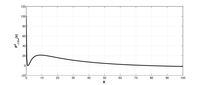
Figure 1: Graph of the function $P^{5}_{-\frac{1}{2}+i}(x)$.

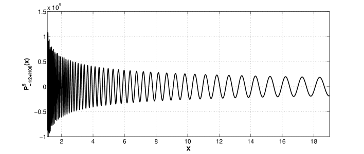
Figure 2: Graph of the function $P^{5}_{-\frac{1}{2}+i100}(x)$.

Next, we are going to describe the theoretical expressions involved in the computation of conical functions:

2.1 Computation of $P^{m}_{-{{\lower 1.80835pt\hbox{$\scriptstyle 1$}}\over{\raise 1.50693pt\hbox{$\scriptstyle 2$}}}+i\tau}(x)$ for $x>0$

Two kind of asymptotic expansions are considered: for large $m$ and for large $\tau$.

2.1.1 Asymptotic expansions for large $m$

For large values of the parameter $m$, asymptotic expansions for $0<x<1$ and $x>1$, respectively, are used:

1. The following asymptotic expansion is valid for $0<x<1$, large positive values of $m$ and uniformly valid for $\tau\geq 0$:

   $$P_{-\frac{1}{2}+i\tau}^{m}(x)\sim\sqrt{\frac{p}{xm}}\,\frac{\Gamma(\frac{1}{2}+m)\,(1-x^{2})^{m/2}\cosh(\pi\tau)e^{-m\phi(t_{0})}}{\pi}\sum_{k=0}^{\infty}\frac{u_{k}(\beta,p)}{m^{k}}.$$ (3)

   The quantities $\beta$, $p$ and $\phi(t_{0})$ are given by

   $$\beta=\frac{\tau}{m},\quad p=\frac{x}{\sqrt{1+\beta^{2}(1-x^{2})}},$$ (4)

   and

   $$\phi(t_{0})=\ln\frac{x(p+1)}{p(\beta^{2}+1)}+\beta\arccos\frac{x(1-p\beta^{2})}{p(1+\beta^{2})}.$$ (5)

   The first few coefficients of the expansion in (3) are

   $$\begin{array}[]{l}u_{0}(\beta,p)=1,\quad u_{1}(\beta,p)=-\displaystyle\frac{-\beta^{2}+5\beta^{2}p^{3}-3\beta^{2}p+3p}{24(\beta^{2}+1)},\\ \\ u_{2}(\beta,p)=\displaystyle\frac{1}{1152(\beta^{2}+1)^{2}}[385\beta^{4}p^{6}+462\beta^{2}(1-\beta^{2})p^{4}-10\beta^{4}p^{3}\\ \\ \quad\quad+(81\beta^{4}-522\beta^{2}+81)p^{2}+6\beta^{2}(\beta^{2}-1)p+\beta^{4}+72\beta^{2}-72].\end{array}$$ (6)

2. For $x>1$, we use a representation in terms of the modified Bessel function $K_{i\tau}(m\zeta)$, which is valid for $m$ positive:

   $$\begin{array}[]{l}P_{-\frac{1}{2}+i\tau}^{m}(x)=\displaystyle\frac{2\Gamma({{\lower 2.58334pt\hbox{$\scriptstyle 1$}}\over{\raise 2.1097pt\hbox{$\scriptstyle 2$}}}+m)\,(x^{2}-1)^{m/2}\,\cosh(\pi\tau)e^{-m\lambda}}{\pi\sqrt{2\pi}\,}\ \Phi(\zeta)\times\\ \\ \quad\quad\quad\left[A_{m}(\beta,\zeta)K_{i\tau}(m\zeta)-B_{m}(\beta,\zeta)K_{i\tau}^{\prime}(m\zeta)\right],\end{array}$$ (7)

   where

   $$\lambda=\frac{1}{2}\left(\ln\frac{x^{2}-1}{\beta^{2}+1}+\beta\arccos\frac{1-\beta^{2}}{1+\beta^{2}}\right),$$ (8)

   $$\beta=\frac{\tau}{m},\quad\Phi(\zeta)=\left(\frac{\zeta^{2}-\beta^{2}}{1+\beta^{2}(1-x^{2})}\right)^{\frac{1}{4}},$$ (9)

   and the functions $A_{m}(\beta,\zeta)$ and $B_{m}(\beta,\zeta)$ have the expansions

   $$A_{m}(\beta,\zeta)\sim\sum_{n=0}^{\infty}\frac{A_{n}(\beta,\zeta)}{m^{n}},\quad B_{m}(\beta,\zeta)\sim\sum_{n=0}^{\infty}\frac{B_{n}(\beta,\zeta)}{m^{n}}.$$ (10)

   These expressions are valid for large $m$.

   In this representation, the parameter $\zeta$ and the coefficients of the expansions are given in two different $x$-regions: $1<x\leq x_{c}$ (the monotonic interval) and $x>x_{c}$ (the oscillatory region), where $x_{c}=\frac{\displaystyle{\sqrt{1+\beta^{2}}}}{\displaystyle{\beta}}$:

   Case $1<x\leq x_{c}$:

   In this case the quantity $\zeta\geq\beta$ is given by the implicit equation

   $$2\left[\sqrt{\zeta^{2}-\beta^{2}}-\beta\arccos(\beta/\zeta)\right]=\ln\frac{p+1}{p-1}-\beta\arccos\frac{\beta^{2}p^{2}-1}{\beta^{2}p^{2}+1},$$ (11)

   where $p$ is given by

   $$p=\frac{x}{\sqrt{1+\beta^{2}(1-x^{2})}}.$$ (12)

   This implicit equation cannot be inverted analitically. Then, a method for computing numerical approximations to the solution of this equation is needed. In the algorithm, we choose Newton’s method given that initial approximations which guarantee convergence of the method can be obtained [5].

   The first few coefficients $A_{n}(\beta,\zeta),B_{n}(\beta,\zeta)$ in (10) are

   $$A_{0}(\beta,\zeta)=1,\quad B_{0}(\beta,\zeta)=0,\quad A_{1}(\beta,\zeta)=\frac{\beta^{2}}{24(1+\beta^{2})},$$ (13)

   $$B_{1}(\beta,\zeta)=-\frac{(5\beta^{2}(W^{3}p^{3}-1-\beta^{2})+3W^{2}(Wp(1-\beta^{2})-1-\beta^{2})\zeta}{24W^{4}(1+\beta^{2})},$$ (14)

   where $p$ is given in (12) and

   $$W=\sqrt{\zeta^{2}-\beta^{2}}.$$ (15)

   Case $x\geq x_{c}$:

   The quantity $\zeta\in[0,\beta]$ is given by the implicit equation

   $$2\left[\sqrt{\beta^{2}-\zeta^{2}}-\beta{\rm arccosh}(\beta/\zeta)\right]=2\,{\rm arccot}\,q-\beta\ln\frac{\beta q+1}{\beta q-1},$$ (16)

   where $q$ is given by

   $$q=\frac{x}{\sqrt{\beta^{2}(x^{2}-1)-1}}.$$ (17)

   As before, this equation is solved by using Newton’s method with appropriated starting values [5].

   The coefficients $A_{0}(\beta,\zeta),B_{0}(\beta,\zeta),A_{1}(\beta,\zeta)$ are as in (13), whereas the coefficient $B_{1}(\beta,\zeta)$ is given by

   $$B_{1}(\beta,\zeta)=-\frac{(5\beta^{2}(V^{3}q^{3}-1-\beta^{2})+3V^{2}(Vq(1-\beta^{2})-1-\beta^{2})\zeta}{24V^{4}(1+\beta^{2})},$$ (18)

   where $V=\sqrt{\beta^{2}-\zeta^{2}}$.

   For the oscillatory case and far away from the transition point between monotonic and oscillatory behaviour of the function ($x>>x_{c}>1$), we also use an asymptotic expansion (valid for large $m$) in terms of elementary functions:

   $$\begin{array}[]{ll}\displaystyle P_{-\frac{1}{2}+i\tau}^{m}(x)\sim 2\sqrt{\frac{q}{mx}}\frac{\left(\beta^{2}+1\right)^{\mu/2}\Gamma\left(\frac{1}{2}+m\right)}{\pi}\cosh(\pi\tau)e^{-\tau(\pi-{\rm arccot}(\beta))}\ \times\\[8.0pt] \quad\quad\quad\quad\quad\quad\quad\quad\displaystyle\left(\cos\chi\sum_{k=0}^{\infty}\frac{v_{k}}{m^{k}}-\sin\chi\sum_{k=0}^{\infty}\frac{w_{k}}{m^{k}}\right).\end{array}$$ (19)

   where

   $$\chi=\mu(\beta\xi-{\rm arccot}\,q)-{{\lower 2.58334pt\hbox{$\scriptstyle 1$}}\over{\raise 3.01385pt\hbox{$\scriptstyle 4$}}}\pi,$$ (20)

   and the other parameters used in the expansion are given by

   $$\beta=\frac{\tau}{\mu},\quad x_{c}=\frac{\sqrt{1+\beta^{2}}}{\beta},\quad\xi={\rm arccosh}\frac{x}{x_{c}},\quad q=\frac{\cosh\xi}{\beta\sinh\xi}.$$ (21)

   The first coefficients of the expansion are

   $$\begin{array}[]{ll}v_{0}=1,\quad w_{0}=0,\\[8.0pt] \displaystyle v_{1}=\frac{\beta^{2}}{24(1+\beta^{2})},\\[8.0pt] \displaystyle w_{1}=-\frac{q(5\beta^{2}q^{2}+3\beta^{2}-3)}{24(1+\beta^{2})},\\[8.0pt] \displaystyle v_{2}=-\frac{385\beta^{4}q^{6}+462\beta^{2}(\beta^{2}-1)q^{4}+(81\beta^{4}-522\beta^{2}+81)q^{2}-\beta^{4}-72\beta^{2}+72}{1152(1+\beta^{2})^{2}},\\[8.0pt] \displaystyle w_{2}=\frac{\beta^{2}q(5\beta^{2}q^{2}+3\beta^{2}-3)}{576(1+\beta^{2})^{2}}.\end{array}$$ (22)

   These coefficients also follow from the coefficents $u_{k}$ given in (4.4) of [5] by writing $p=iq$. Then

   $$v_{k}=(-1)^{k}\Re u_{k},\quad w_{k}=(-1)^{k}\Im u_{k}.$$ (23)

2.1.2 Asymptotic expansions for large $\tau$

In order to obtain this expansion, we take the integral representation

$$\begin{array}[]{ll}\displaystyle\Gamma\left({{\lower 2.58334pt\hbox{$\scriptstyle 1$}}\over{\raise 3.01385pt\hbox{$\scriptstyle 2$}}}+\mu\right)\sqrt{\pi/2}\,\sinh^{\mu}\beta\,P_{-\frac{1}{2}+i\tau}^{-\mu}\left(\cosh\beta\right)=\\ \quad\quad\quad\quad\quad\displaystyle\int_{0}^{\beta}\left(\cosh\beta-\cosh t\right)^{\mu-\frac{1}{2}}\cos\tau t\,dt,\quad\Re\mu>-{{\lower 2.58334pt\hbox{$\scriptstyle 1$}}\over{\raise 3.01385pt\hbox{$\scriptstyle 2$}}},\end{array}$$ (24)

which is given in [7, p. 184].

The large $\tau$ asymptotics follows from applying the method of stationary phase; see [11, §II.3].

We have the following result

$$\Gamma\left({{\lower 2.58334pt\hbox{$\scriptstyle 1$}}\over{\raise 3.01385pt\hbox{$\scriptstyle 2$}}}+\mu\right)\sqrt{\pi/2}\,\sinh^{\mu}\beta\,P_{-\frac{1}{2}+i\tau}^{-\mu}\left(\cosh\beta\right)\sim\sum_{n=0}^{\infty}\frac{A_{n}}{\tau^{n+1}}+\sum_{n=0}^{\infty}\frac{B_{n}}{\tau^{n+\mu+\frac{1}{2}}},$$ (25)

where

$$A_{n}=\left.-\sin(n\pi/2)\frac{d^{n}}{dt^{n}}\left(\cosh\beta-\cosh t\right)^{\mu-\frac{1}{2}}\right|_{t=0},$$ (26)

and

$$B_{n}=\left.\cos\chi_{n}\,\frac{\Gamma(n+\mu+\frac{1}{2})}{n!}\frac{d^{n}}{dt^{n}}\left(\frac{\cosh\beta-\cosh t}{\beta-t}\right)^{\mu-\frac{1}{2}}\right|_{t=\beta},$$ (27)

where

$$\chi_{n}={{\lower 2.58334pt\hbox{$\scriptstyle 1$}}\over{\raise 3.01385pt\hbox{$\scriptstyle 2$}}}\left(n-\mu-{{\lower 2.58334pt\hbox{$\scriptstyle 1$}}\over{\raise 3.01385pt\hbox{$\scriptstyle 2$}}}\right)\pi+\beta\tau.$$ (28)

The coefficients $A_{n}$ vanish for even $n$, because of the sine function. They vanish also for odd $n$, because in that case the derivatives vanish at $t=0$.

The expansion in (25), valid for arguments greater than 1 and large $\tau$, can be written in the form

$$\begin{array}[]{lll}P_{-\frac{1}{2}+i\tau}^{m}\left(\cosh\beta\right)&\sim&\sqrt{\frac{\displaystyle{2}}{\displaystyle{\pi\sinh\beta}}}\cosh(\pi\tau)\frac{\displaystyle{|\Gamma(m+1/2+i\tau)|^{2}}}{\displaystyle{\pi}}\times\\ &&\sum_{n=0}^{\infty}\cos\chi_{n}\left(m+{{\lower 2.58334pt\hbox{$\scriptstyle 1$}}\over{\raise 2.1097pt\hbox{$\scriptstyle 2$}}}\right)_{n}\frac{\displaystyle{b_{n}}}{\displaystyle{\tau^{n+m+\frac{1}{2}}}},\end{array}$$ (29)

where the first few coefficients $b_{n}$ are given by

$$\begin{array}[]{ll}\displaystyle b_{0}=1,\\[8.0pt] \displaystyle b_{1}=\frac{(2m-1)x}{4\sinh\beta},\\[8.0pt] \displaystyle b_{2}=\frac{(2m-1)(-8+(6m-1)x^{2})}{96\sinh^{2}\beta},\\[8.0pt] \displaystyle b_{3}=\frac{(2m-1)x((-1+4m^{2})x^{2}+16-16m)}{384\sinh^{3}\beta},\end{array}$$ (30)

and where $\left(m+{{\lower 2.58334pt\hbox{$\scriptstyle 1$}}\over{\raise 2.1097pt\hbox{$\scriptstyle 2$}}}\right)_{n}$ is the Pochhammer symbol of $m+{{\lower 2.58334pt\hbox{$\scriptstyle 1$}}\over{\raise 2.1097pt\hbox{$\scriptstyle 2$}}}$.

As this expansion holds for small $m$, we will use it for $m=0,1$; then, if larger values of $m$ are wanted, we will apply forward recursion with the $m$-three term recurrence relation, as we will later discuss.

2.2 Computation of $P^{m}_{-{{\lower 1.80835pt\hbox{$\scriptstyle 1$}}\over{\raise 1.50693pt\hbox{$\scriptstyle 2$}}}+i\tau}(x)$ for $-1<x<0$

Conical functions in the interval $x\in(-1,\,0)$ are computed by means of a stable integral representation as described in [5]. The starting point is the following integral representation:

$$P_{-\frac{1}{2}+i\tau}^{m}(x)=\frac{\Gamma({{\lower 2.58334pt\hbox{$\scriptstyle 1$}}\over{\raise 2.1097pt\hbox{$\scriptstyle 2$}}}+m)\,(1-x^{2})^{m/2}\cosh(\pi\tau)}{\pi\sqrt{2\pi}}\int_{-\infty}^{\infty}e^{-m\phi(t)}\frac{dt}{\sqrt{x+\cosh t}},$$ (31)

where

$$\phi(t)=\ln(x+\cosh t)-i\beta t,\quad\beta=\frac{\tau}{m}.$$ (32)

In this form, this representation is not suitable for numerical computation because of the factor $e^{im\beta t}$ in the integrand: this factor introduces oscillations which could be very strong for large values of $\tau$. Steepest descent methods [4, Ch. 5] can be used for transforming this integral into a stable representation, where oscillations are under control. In this way, it is possible to obtain the following representation, valid for $-1<x<0$:

$$\begin{array}[]{ll}P_{-\frac{1}{2}+i\tau}^{m}(x)&=\frac{\displaystyle{\Gamma({{\lower 2.58334pt\hbox{$\scriptstyle 1$}}\over{\raise 3.01385pt\hbox{$\scriptstyle 2$}}}+m)\,(1-x^{2})^{m/2}}}{\displaystyle{\pi\sqrt{2\pi}}}2\cosh(\pi\tau)e^{-\mu\phi(t_{0})}\displaystyle\sqrt{\frac{p(1+\beta^{2})}{x(p+1)}}\\ &\displaystyle\int_{0}^{\infty}e^{-(m+\frac{1}{2})\psi_{r}(s)}\cos((m+{{\lower 2.58334pt\hbox{$\scriptstyle 1$}}\over{\raise 3.01385pt\hbox{$\scriptstyle 2$}}})\psi_{i}(s))\,ds,\end{array}$$ (33)

where

$$\beta=\frac{\tau}{m},\quad p=\frac{x}{\sqrt{1+\beta^{2}(1-x^{2})}},$$ (34)

$$\phi(t_{0})=\ln\frac{x(p+1)}{p(\beta^{2}+1)}+\beta\arccos\frac{x(1-p\beta^{2})}{p(1+\beta^{2})}.$$ (35)

and

$$\begin{array}[]{l}\displaystyle\psi_{r}(s)={{\lower 2.58334pt\hbox{$\scriptstyle 1$}}\over{\raise 3.01385pt\hbox{$\scriptstyle 2$}}}\ln\left(1+\frac{4(1+\beta^{2})}{1+p}\sigma^{2}+\frac{4(1+\beta^{2})(1+p^{2}\beta^{2})}{(1+p)^{2}}\sigma^{4}\right),\\ \\ \displaystyle\psi_{i}(s)=\arctan\frac{\beta(1+p)\sinh s}{1+p+(1-p\beta^{2})\sinh^{2}(s/2)}-\beta s,\end{array}$$ (36)

where $\sigma=\sinh({{\lower 2.58334pt\hbox{$\scriptstyle 1$}}\over{\raise 2.1097pt\hbox{$\scriptstyle 2$}}}s)$.

2.3 Three-term recurrence relations

Conical functions $P_{-1/2+i\tau}^{m}(x)$ satisfy three-term recurrence relations, which are given by:

$$P_{-\frac{1}{2}+i\tau}^{m+1}(x)+\frac{\displaystyle{2mx}}{\displaystyle{\sqrt{1-x^{2}}}}P_{-\frac{1}{2}+i\tau}^{m}(x)-\left((m-{{\lower 2.58334pt\hbox{$\scriptstyle 1$}}\over{\raise 3.01385pt\hbox{$\scriptstyle 2$}}})^{2}+\tau^{2}\right)P_{-\frac{1}{2}+i\tau}^{m-1}(x)=0$$ (37)

for $x\in(-1,1)$ and

$$P_{-\frac{1}{2}+i\tau}^{m+1}(x)-\frac{\displaystyle{2mx}}{\displaystyle{\sqrt{x^{2}-1}}}P_{-\frac{1}{2}+i\tau}^{m}(x)+\left((m-{{\lower 2.58334pt\hbox{$\scriptstyle 1$}}\over{\raise 3.01385pt\hbox{$\scriptstyle 2$}}})^{2}+\tau^{2}\right)P_{-\frac{1}{2}+i\tau}^{m-1}(x)=0$$ (38)

for $x>1$.

These recurrence relations can be used, starting from two initial values, for computing the functions when they are applied in the direction of stable recursion: either backward or forward. Also, we will use these relations as a test for the computations.

The stability analysis based on Perron’s theorem discussed in [5], revealed that backward (forward) recursion was generally stable for $x>0$ ($x<0$). However and similarly to other special functions, recurrence relations in the oscillatory regime of the conical functions ($x>x_{c}>1$) are not bad conditioned in both backward and forward directions; then, both recursions are possible. We will use this property in combination to the asymptotic expansion given in (29) for computing conical functions for large $\tau$ in the oscillatory regime of the functions.

3 Overview of the software structure

The Fortran 90 package includes the main module Conical, which includes the routine conic.

In the module Conical, the auxiliary module Someconstants is used. This is a module for the computation of the main constants used in the different routines. The routines included in auxil.f90 are also used in the module Conical. Among them, there is a Fortran 90 version of a Fortran 77 routine for computing the modified Bessel functions $K_{ia}(x)$ and its derivative $K^{\prime}_{ia}(x)$, developed by the authors [3], [2].

4 Description of the individual software components

The Fortran 90 module Conical includes the public routine conic which computes the conical functions $P^{m}_{-\frac{1}{2}+i\tau}(x)$, $x>-1$, $m\geq 0$, $\tau>0$. The calling sequence of this routine is

   CALL  conic(x,mu,tau,pmtau,ierr)
  

where the input data are: $x$, $mu$ and $tau$ (arguments of the functions). The outputs are the error flag $ierr$ and the function value $pmtau$. The possible values of the error flag are: $ierr=0$, successful computation; $ierr=1$, computation failed due to overflow/underflow; $ierr=2$, arguments out of range.

5 Testing the algoritm

Two kind of tests have been considered for testing the accuracy of the computed values of the conical functions: direct comparison against Maple and a single step of the three-term recurrence relations (37) and (38). At most of the points of the tested parameter space $(x,\tau,m)$ the comparison against Maple shows that the accuracy was $\sim 10^{-12}$ or better ($10^{-13}-10^{-14}$ in $-1<x<0$, included in the monotonic region). It is important to point out that for $x>1$, asymptotic expansions using the modified Bessel functions $K_{ia}(x)$ and $K^{\prime}_{ia}(x)$ (7) are considered and that the accuracy in the computation of these functions is $\sim 5\times 10^{-13}$, as explained in [2]. So, the accuracy for computing these functions limit the attainable accuracy in the computation of conical functions. On the other hand, at some points of the oscillatory region of the conical functions, the tested accuracy was $\sim 10^{-10}$. This is apparent in Figure (3), where points in the $(x,\tau)$-plane with a relative error (in comparison with the Maple value) $\sim 10^{-10}$ in the computation of $P^{95}_{-\frac{1}{2}+i\tau}(x)$, are plotted. The figure also shows the curve $y=\sqrt{1+\beta^{2}}/\beta$, where $\beta=\tau/95$. This curve is the frontier between the monotonic and the oscillatory regions for the conical function $P^{95}_{-\frac{1}{2}+i\tau}(x)$. Additionally, the approximations used in the algorithm for $x>1$ are indicated in the figure. As can be seen, the density of plotted points is larger in the region where asymptotic expansions in terms of modified Bessel functions are used. Finally, it is important also to note that in the oscillatory region the zeros of the conical functions are found and at these points relative error losses its meaning.

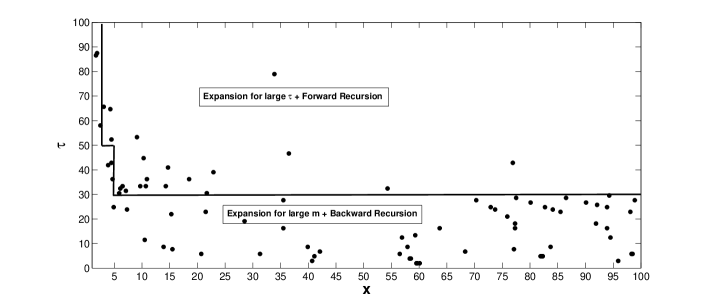
Figure 3: Points in the $(x,\tau)$-plane ($x>1$) where the relative error in comparison with the Maple value in the computation of $P^{95}_{-\frac{1}{2}+i\tau}(x)$ is $\sim 10^{-10}$. At the rest of tested points in the $(x,\tau)$-plane, the accuracy was found $\sim 10^{-12}$ or better. The curve $y=\sqrt{1+\beta^{2}}/\beta$, where $\beta=\tau/95$, and the regions where different approximations are used in the algorithm for $x>1$, are also shown in the figure.

6 Test run description

The Fortran 90 test program testcon.f90 includes the computation of 25 function values and their comparison with the corresponding pre-computed results. Also, a single step of the three-term recurrence relations (37) and (38) is tested for several values of the parameters $(x,\,\tau,\,m)$.

7 Acknowledgements

The authors thank the referee for useful comments. The authors acknowledge financial support from Ministerio de Ciencia e Innovación, project MTM2009-11686. NMT acknowledges financial support from Gobierno of Navarra, Res. 07/05/2008.

References

• [1] T.Β M. Dunster. Legendre and related functions. In NIST handbook of mathematical functions, pages 351–381. Cambridge University Press, New York, 2010.
• [2] A.Β Gil, J.Β Segura, and N.Β M. Temme. Algorithm 831: modified Bessel functions of imaginary order and positive argument. ACM Trans. Math. Softw., 30(2):159–164, 2004.
• [3] A.Β Gil, J.Β Segura, and N.Β M. Temme. Computing solutions of the modified Bessel differential equation for imaginary orders and positive arguments. ACM Trans. Math. Softw., 30(2):145–158, 2004.
• [4] A.Β Gil, J.Β Segura, and N.Β M. Temme. Numerical methods for special functions. Society for Industrial and Applied Mathematics (SIAM), Philadelphia, PA, 2007.
• [5] Amparo Gil, Javier Segura, and NicoΒ M. Temme. Computing the conical function $P^{\mu}_{-1/2+i\tau}(x)$. SIAM J. Sci. Comput., 31(3):1716–1741, 2009.
• [6] K.S. KΓΆlbig. A program for computing the conical functions of the first kind ${P}^{m}_{-1/2+i\tau}(x)$ for $m=0$ and $m=1$. Comput. Phys. Commun., 23:51–61, 1981.
• [7] W.Β Magnus, F.Β Oberhettinger, and R.P. Soni. Formulas and theorems for the special functions of mathematical physics. Third enlarged edition. Die Grundlehren der mathematischen Wissenschaften, Band 52. Springer-Verlag New York, Inc., New York, 1966.
• [8] A.Β Passian, S.Β Koucheckian, S.Β B. Yakubovich, and T.Β Thundat. Properties of index transforms in modeling of nanostructures and plasmonic systems. J. Math. Phys., 51(2):023518, 30, 2010.
• [9] A.Β Stebbins and R.R. Caldwell. No very large scale structure in an open universe. Phys. Rev. D, 52(6):3248–3264, 1995.
• [10] E.Β Thebault, J.J. Schott, M.Β Mandea, and J.P. Hoffbeck. A new proposal for spherical cap harmonic analysis. Geophys. J. Int., 159:83–103, 2004.
• [11] R.Β Wong. Asymptotic approximations of integrals, volumeΒ 34 of Classics in Applied Mathematics. Society for Industrial and Applied Mathematics (SIAM), Philadelphia, PA, 2001. Corrected reprint of the 1989 original.