Feshbach Resonance without a Closed Channel Bound-State

Abstract

The physics of Feshbach resonance is analyzed using an analytic expression for the $s$-wave scattering phase-shift and the scattering length $a$ which we derive within a two-channel tight-binding model. Employing a unified treatment of bound states and resonances in terms of the Jost function, it is shown that for strong inter-channel coupling, Feshbach resonance can occur even when the closed channel does not have a bound state. This may extend the range of ultra-cold atomic systems that can be manipulated by Feshbach resonance. The dependence of the sign of $a$ on the coupling strength in the unitary limit is elucidated. As a by-product, analytic expressions are derived for the background scattering length, the external magnetic field at which resonance occurs, and the energy shift $\varepsilon-\varepsilon_{B}$, where $\varepsilon$ is the scattering energy and $\varepsilon_{B}$ is the bound state energy in the closed channel (when there is one).

Introduction.— Feshbach resonance (FR) enables manipulation of the interactions between ultra-cold atoms, e.g., it allows a repulsive gas to be transformed into an attractive one and vice-versa Feshbach ; Kerman ; Julienne1 ; CCT ; Chin_10 ; Blatt_11 ; Jones_06 , as in a BEC-BCS crossover Regal_04 . The paradigm of FR, as in the low energy collision of two ultra-cold atoms, involves the coupling of an open channel, $o$, and a bound state at energy $\varepsilon_{B}$ in (another) closed channel, $c$, giving rise to resonant variations of the $s$-wave scattering length $a$ CCT . This resonance occurs when $\varepsilon_{B}\approx\varepsilon$ where $\varepsilon$ is the scattering energy, namely, when the energy of the closed channel bound state is close to the threshold of the open channel. This condition can be experimentally implemented by varying an external parameter, such as a static magnetic field $B$, so that the bound state energy is swept through resonance. As we show below, this paradigm can be extended to the case where the closed channel does not have a bound state.

FR is usually formulated as a two-channel scattering problem, which establishes the relation between the bare parameters of the scattering problem (electronic potentials, coupling strength, scattering energy and external fields) and the physically relevant observables (e.g., the scattering length versus external field, $a(B)$, the bound states of the coupled system, etc.). In this context, it is useful to consider a two-channel model that allows the derivation of analytical expressions of these observables in order to elucidate their relation to the bare parameters. Such a model is not intended to analyze a specific system in detail in which the intra-channel potentials and the inter-channel coupling have a definite form appropriate for the system under study. Rather, it should be sufficiently general and simple and, at the same time, encode the underlying physics. The basic ingredients of a two channel $s$-wave scattering problem designed to analyze a FR include: (1) The intra-channel potentials $v_{o}(r)$ of the open channel and $v_{c}(r)$ of the closed channel (here $r$ is the distance between the two atoms). (2) The inter-channel coupling potential $w(r)$ (for simplicity we take a constant coupling strength $\tau$). (3) An external tunable parameter controlling the energy difference $v\equiv v_{c}(r)-v_{o}(r)$ as $r\to\infty$. Experimentally, $v$ is often tuned by varying an external magnetic field, $v=\alpha B$, where the constant $\alpha$ depends on the specific system. Thus, knowing the value $v=v_{0}$ for which the system has a FR is equivalent to finding the magnetic field $B_{0}$ at which the scattering length is infinite.

Our main objective here is to show that FR can occur even when the closed channel does not have a bound state, or even when the atom-atom potential in this channel is repulsive. The motivation for addressing this question is evident: this will demonstrate that systems for which a transition from an attractive gas of atoms to a repulsive gas are feasible even for systems for which $v_{c}(r)$ does not support a bound state. Using a simple model, we show that this is indeed the case; it is possible to obtain a FR and a bound state of the coupled-channel system for large enough coupling $\tau$ of the closed and open channels, even when there is no bound state in the closed channel. As a by product, analytic expressions are derived for the basic physical observables related to FR in terms of the parameters of the scattering problem and a unified treatment of bound states and resonances is carried out in terms of the Jost function.

The two-channel scattering problem.— The $s$-wave two-channel scattering problem between two atoms a distance $r$ can be mapped onto a single-particle scattering problem in the center of mass coordinate system governed by the Schrödinger equation (in abstract form),

$$\binom{H_{o}\ w^{\dagger}}{\ w\ \ H_{c}}\binom{u_{o}}{u_{c}}=\varepsilon\binom{u_{o}}{u_{c}}=k^{2}\binom{u_{o}}{u_{c}}~{}.$$ (1)

$H_{o}=-\tfrac{d^{2}}{dr^{2}}+v_{o}(r)$ and $H_{c}=-\tfrac{d^{2}}{dr^{2}}+v_{c}(r)$ are the Hamiltonians (in $r$ space) for the open and closed channels composed of the kinetic energy operator and intra-channel potentials $v_{o}$ and $v_{c}$, and $\varepsilon=\varepsilon_{k}=k^{2}$. The open and closed channels are coupled by the potential $w(r)$. The boundary conditions satisfied by the closed and open components of the exact wave function are $u_{o}(0)=u_{c}(0)=0$, $u_{c}(r)_{r\to\infty}=Ae^{-\kappa r}$, and $u_{o}(r)_{r\to\infty}=B\sin[kr$+$\delta(k)]$. Here $\kappa(\varepsilon_{k})>0$, $A$ and $B$ are energy dependent constants and $\delta(k)$ is the scattering phase shift. The $s$-wave scattering length is given by

$$a=-\lim_{k\to 0}\frac{\tan\delta(k)}{k},$$ (2)

In the standard picture of FR, the closed channel, when uncoupled from the open channel, is assumed to have a bound state $|B\rangle$ at energy $\varepsilon_{B}<v_{c}(\infty)$ and continuum states, $\{|p\rangle\}$ at energies $\{\epsilon_{p}>v_{c}(\infty)\}$. The scattering states of $H_{o}$ are defined as $H_{o}|k\rangle=\varepsilon|k\rangle=k^{2}|k\rangle$ (assuming $v_{o}(\infty)=0$ for simplicity). Eliminating $|u_{c}\rangle$ from the set of coupled equations (1) results in a single equation for $|u_{o}\rangle$, $[H_{o}+v_{\mathrm{eff}}(\varepsilon)]|u_{o}\rangle=\varepsilon|u_{o}\rangle,$ with an effective potential, $v_{\mathrm{eff}}(\varepsilon)=wG_{c}(\varepsilon)w^{\dagger}$, where $G_{c}(\varepsilon)=(\varepsilon-H_{c})^{-1}$. The $T$ matrix associated with $v_{\mathrm{eff}}(\varepsilon)$ is formally given by $T(\varepsilon)=[1-G_{o}(\varepsilon)v_{\mathrm{eff}}(\varepsilon)]^{-1}$, and, by definition, $a=-C\lim_{k\to 0}\langle k|T(\varepsilon)|k\rangle$, where $C>0$ is a kinematic constant.

For example, a particularly simple model takes $v_{o}(r)$ and $v_{c}(r)$ to be spherical square wells of range $R$, while $w(r)$ couples the two channel only at $R$. Explicitly,

$$v_{c}(r)=v\Theta(r-R)+(v-\Delta)\Theta(R-r)$$

$$v_{o}(r)=-\Lambda\Theta(R-r),\ \ w(r)=\tau\,\delta(r-R),$$ (3)

where $\tau$ is the coupling strength. Despite being a simple model, an exact solution of the scattering problem requires solving a set of coupled transcendental equations. Its numerical solution supp_mat confirms the analytical results obtained within the tight-binding (TB) model to which we now turn.

Tight-Binding Model.— Starting from the continuous model, we discretize the radial coordinate, $r\to n$, where $n>0$ is an integer, and replace $-\frac{d^{2}}{dr^{2}}$ by a second-order difference operator Molmer . In second quantization it translates as a hopping term, $-(\sum_{n\geq 1}a_{n}^{\dagger}a_{n+1}+h.c.)$, where $a_{n}$ and $a_{n}^{\dagger}$ are the annihilation and creation operators of the scattered particle on the positive integer grid-sites $n>0$. The potentials are,

$$v_{c}(n)=(v-\Delta)\delta_{n,1}+v\Theta(n-1),$$

$$v_{o}(n)=-\Lambda\delta_{n,1},\quad w(n)=\tau\delta_{n,1}.$$ (4)

After treating the closed and open channels separately, we will solve the coupled-channel scattering problem.

The Hamiltonian of the closed channel is,

$$H_{c}=(v-\Delta)a_{1}^{\dagger}a_{1}+\sum_{n>1}[v\,a^{\dagger}_{n}a_{n}-(a_{n}^{\dagger}a_{n-1}+h.c.)].$$ (5)

If the well-depth $\Delta>0$, the potential is attractive at site $n=1$. The potential height $v$ for $n>1$ is experimentally tunable (e.g., via magnetic field). Let $f_{n}$ be the amplitude of the wave function at site $n$. For a bound state with binding energy $\varepsilon_{B}$, $f_{n}=A_{c}\,e^{-\kappa(n-2)}\ (n>1)$ with $\kappa>0$ and $A_{c}$ is a constant. Therefore, for $n>1$ (i.e., outside the range of the attractive potential), $f_{2}=A,\ \ f_{3}=A\,e^{-\kappa}$ and $\varepsilon_{B}=v-2\cosh\kappa)$. Simple manipulations yield,

$$\kappa=\log\Delta>0~{}\Rightarrow\Delta\geq 1,\quad\varepsilon_{B}=v-\left[\Delta+\frac{1}{\Delta}\right].$$ (6)

Thus, there is a threshold potential depth $\Delta>1$ for having an $s$-wave bound state. A similar scenario occurs also in a 3D continuous geometry, in contradistinction to symmetric 1D or 2D potentials, where any attractive potential of whatever strength supports a bound state. In the model treated here, at most one bound state can occur Wasak_13 . An artifact of the TB model is that for a repulsive potential with $\Delta<-1$, the closed channel does have a bound state above the upper band edge Manuel . To avoid this, we will restrict the potential depth to $\Delta>-1$. To summarize, for $\Delta>1$ the closed channel has a bound state while for $1>\Delta>0$, $v_{c}$ is attractive but there is no bound state. Moreover, for $0>\Delta>-1$, $v_{c}$ is repulsive and there is no bound state.

For the open channel we use $b^{\dagger}_{n}$ and $b_{n}$ as creation and annihilation operators. The Hamiltonian is,

$$H_{o}=-\Lambda b_{1}^{\dagger}b_{1}-\sum_{n\geq 1}(b^{\dagger}_{n+1}b_{n}+h.c.).$$ (7)

For $\Lambda>1$ the open channel has a bound state, for $1>\Lambda>0$, $v_{o}$ is attractive, but there is no bound state, whereas for $0>\Lambda>-1$, $v_{o}$ is repulsive and there is no bound state. The wave function on site $n\geq 1$ is $g_{n}=A_{o}\sin[k(n-1)+\delta(k)]$, where $A_{o}$ is a constant. The continuous spectrum is a band of energies,

$$\varepsilon_{k}=-2\cos k~{},\ \Rightarrow\ -2\leq\varepsilon_{k}\leq 2,$$ (8)

so that the lowest threshold for propagation is $\varepsilon_{k=0}=-2$.

Now, consider the coupled-channel system. The Hamiltonian is,

$$H=H_{c}+H_{o}+\tau(a_{1}^{\dagger}b_{1}+h.c.)~{}.$$ (9)

In a scattering scenario, the effective particle approaches the “origin”, $n=0$, in the open channel from right to left at a given energy, $\varepsilon_{k}=-2\cos k$, and is reflected back (rightward) into the open channel. The reflection amplitude, equivalently the $S$ matrix, is $S=e^{2i\delta(k)}$, where $\delta(k)$ is the $s$-wave phase shift from which $a$ is computed as in Eq. (2). $f_{n}$ and $g_{n}$ are the amplitudes of the wave function on site $n$ for the closed and open channels respectively [analogous of $u_{c}(r)$ and $u_{o}(r)$ in the continuous model]. The “asymptotic” forms of $f_{n}$ and $g_{n}$ are,

$$f_{n}=A_{c}e^{-\kappa n},\ \ g_{n}=\sin[k(n-1)+\delta(k)],\ \ (n>1),$$ (10)

where $\kappa$ is related to $\varepsilon_{k}$ as, $2\cosh\kappa=v-\varepsilon_{k}\geq 2$. Thus, the “non-leakage” condition, $v-\varepsilon_{k}>2$, guarantees that propagation in the closed channel is evanescent. Unlike Eq. (34d), here $\kappa$ is independent of the depth $\Delta$ of $v_{c}$.

Solution.— Solving the TB equations we obtain a relatively simple expression for $\tan\delta(k)$, independent of sgn$(\tau)$. Writing $\tan\delta(k)=N/D$ and $q(v,k)=\sqrt{(v-\varepsilon_{k})^{2}-4}$, we find

$$N(k,\tau,v,\Delta,\Lambda)=\{2\tau^{2}+\Lambda[v-\varepsilon_{k}+q(v,k)-2\Delta]\}\sin k,$$

$$D(k,\tau,v,\Delta,\Lambda)=q(v,k)+v-2\Delta+(\tau^{2}-1)\varepsilon_{k}$$

$$\quad+\Lambda[(2\Delta-v)\cos k-q(v,k)\cos k-\cos 2k-1].$$ (11)

Because $N(k,...)=-N(-k,...)$ and $D(k,...)=D(-k,...)$, $\delta(-k)=-\delta(k)+n\pi$ ($n=$ integer). Extracting $\delta(k)$ from $\tan\delta(k)$ requires a reference; in the continuum version, $\delta(\infty)=0$, but in TB, “$\infty$” refers to $k=\pi$.

Next we find at what potential $v=v_{0}(\tau,\Delta,\Lambda)$ we arrive at a FR as $k\to 0$. This is equivalent to finding the value of the magnetic field $B_{0}$ for which there is a FR and $|a|\to\infty$ (an experimentally relevant challenge). Because $N(0,...)=0$, a necessary condition on $v_{0}$ for achieving $|a|=-\lim_{k\to 0}[|\tan\delta(k)|/k]=\infty$ is $D(0,\tau,v_{0},\Delta,\Lambda)=0$. From Eq. (Feshbach Resonance without a Closed Channel Bound-State) we easily obtain,

$$v_{0}(\tau,\Delta,\Lambda)=\frac{[\Lambda-1+\tau^{2}+\Delta(1-\Lambda)]^{2}}{[\Delta(1-\Lambda)+\tau^{2}](1-\Lambda)}.$$ (12)

Equation (Feshbach Resonance without a Closed Channel Bound-State) is also a sufficient condition for $|a|=\infty$ because $D(k,\tau,v_{0},\Delta,\Lambda)$ vanishes as $k^{2}$ when $k\to 0$. Therefore, when $v=v_{0}$, the denominator $D$ in Eq. (Feshbach Resonance without a Closed Channel Bound-State) vanishes faster than the numerator $N\propto\sin k$ (see Sec. III of the supplementary material), and thus, $|a|\to\infty$. Hence, for a given $\tau,\Delta,\Lambda$, one can tune $v\to v_{0}(\tau,\Delta,\Lambda)$, Eq. (12), in order to achieve a FR [equivalently, $|\tan\delta(0)|=\infty$].

The discussion following Eq. (9) dictates that $v_{0}$ must be positive in order to guarantee the non-leakage condition of the closed channel as discussed after Eq. (10). Inspecting the expression (12) for $v_{0}$, we see that it is reasonable to constrain $\Lambda<1$. Under this condition, the open channel potential is attractive (equivalently, $\Lambda>0$) but it does not support a bound state ($\Lambda<1$).

In order to substantiate our main result we need to understand the relationship between the occurrence of bound states in a coupled-channel system and FRs. A uniform treatment of resonances and bound states of the coupled-channel system is achievable in terms of the Jost function. For $v\neq v_{0}(\tau,\Delta,\Lambda)$ [Eq. (12)], resonances and/or bound states of the coupled system exist for $\varepsilon\neq-2$. To explore this regime we use the Jost function, defined (for fixed $\tau,\Delta,\Lambda$) as,

$$f(k,v)\equiv D(k,\tau,v,\Delta,\Lambda)-iN(k,\tau,v,\Delta,\Lambda).$$ (13)

The $S$ matrix is given in terms of the Jost function as, $S=e^{2i\delta}=(1+i\tan\delta)/(1-i\tan\delta)=f(-k,v)/f(k,v)$. The Jost function in ordinary potential scattering is discussed in textbooks on scattering theory, e.g. Taylor , but here it is formulated and exactly calculated for a ‘non-ordinary’ scattering problem with an effective energy-dependent potential. Considered as a function of the complex variable $z=k+iq$ ($0\leq k\leq\pi,\ -\infty<q<\infty$), $f(z,v)$, is well defined on the imaginary $z$ axis, $z=iq$, where it is real. Solving $f(iq,v)=0$ gives the position $q(v)$ that is a pole of the $S$ matrix on the imaginary axis in the $z$ plane. An $s$-wave bound state appears as an isolated zero of $f(iq,v<v_{0})$ with $q>0$, whereas an $s$-wave resonance appears as an isolated zero of $f(iq,v>v_{0})$ with $q<0$. In both cases, the energy equals $-2\cosh q<\varepsilon_{0}=-2$ (namely, below the continuum threshold), but, strictly speaking, the resonance energy is located on the second Riemann sheet in the complex energy plane. Finally, a FR is a zero of $f(iq,v_{0})$ occurring at $q\to 0$. Thus, a small upward shift of $v_{c}$ turns a zero-energy bound state at $q=0^{+}$ into a zero-energy (Feshbach) resonance at $q=0^{-}$.

We are now in a position to derive our main result. Equation (12) shows that for fixed $0<\Lambda<1$, it is possible to modify $\Delta\to\Delta^{\prime}$ and $\tau\to\tau^{\prime}$ in such a way that $\tau^{\prime 2}=\tau^{2}+(\Delta-\Delta^{\prime})(1-\Lambda)$, without affecting $v_{0}$. We employ this property for the case $\Delta>1$ (the closed channel has a bound state) and $\Delta^{\prime}<1$ (no bound state in the closed channel), or even $-1<\Delta^{\prime}<0$. The equality $v_{0}(\tau,\Delta,\Lambda)=v_{0}(\tau^{\prime},\Delta^{\prime},\Lambda)$ guarantees that in both cases FR exists as is evident from Fig. 1 and as is explained in the caption. However, only the case $\Delta>1$ is commensurate with the paradigm of the FR spelled at the introduction, according to which a bound state in the closed channel is responsible for FR.

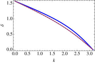
Figure 1: Phase shift $\delta(k)$ versus $k$, Eq. (Feshbach Resonance without a Closed Channel Bound-State). Solid curve: $\tau=2,\ \Delta=1.1>1,\Lambda=0.2$ (the closed channel has a bound state). Dashed curve: $\tau=2.227,\Delta=-0.1<0,\Lambda=0.2$ (the atom-atom potential in the closed channel is repulsive). In both cases $v_{0}(\tau,\Delta,\Lambda)$ defined in Eq. (12) is equal to 4.264 and $\delta(0)=\pi/2$, implying a FR. The curves are virtually identical for small $k$ because $v_{0}$ is determined by the phase shift near $k=0$.

This somewhat unexpected result is not an artifact of the TB model. In the supplementary material we present a formal proof for a continuous model and substantiate it numerically. To get a simpler (albeit intuitive) physical picture, consider the equation for the open channel $[H_{o}+v_{\mathrm{eff}}(\varepsilon)]\psi_{o}=\varepsilon\psi_{o}$ where $v_{\mathrm{eff}}(x)=w(x-H_{c})^{-1}w^{\dagger}$. If $H_{c}$ has only a continuous spectrum starting at $\epsilon_{0}>0$ (i.e., $H_{c}$ does not have a bound state), then for every $x<0$ we have $v_{\mathrm{eff}}(x)=-w[\sqrt{H_{c}-x}\sqrt{H_{c}-x}]^{-1}w^{\dagger}$ that is a negative definite hermitian operator. Thus, $v_{\mathrm{eff}}(x)$ is a non-local attractive potential. By properly tuning the coupling strength $\tau^{2}$ it is possible to get a zero-energy bound state for $x=\varepsilon=0^{-}$. As indicated in the discussion of the Jost function above, a small upward shift of the closed channel potential $v_{c}$ moves a zero-energy bound state into a zero-energy resonance, i.e., a FR. Summarizing, the physical picture of this new type of FR is as follows: A strong coupling leads to a zero-energy bound state in the equation of the open channel alone (that includes an attractive potential $v_{\mathrm{eff}}$). Then, a slight upward shift of the closed channel potential turns this zero-energy bound state into a FR.

Right at FR, $|a|=\infty$. Properties of a unitary gas, where $|a|\approx\infty$, are of great interest in cold atom physics Castin . Direct analysis of Eq. (Feshbach Resonance without a Closed Channel Bound-State) (see Sec. III of the supplementary material) shows that the unitary gas is attractive or repulsive depending upon the coupling strength $\tau$. Specifically, there exists a threshold $\tau_{0}$ such that at the FR, $a=-\infty\ (+\infty)$ for $\tau>\tau_{0}$ ($\tau<\tau_{0}$).

Finally, we use our analytic results within the TB model to derive explicit expressions for several important quantities related to FR. The simple expressions for these quantities teach us directly how these physical observables depend on the parameters $v,\Delta,\Lambda$ and $\tau$.
(1) The functional dependence of $a$ on $v$ (that is proportional to the applied magnetic field $B$) is of utmost importance. Using expression (Feshbach Resonance without a Closed Channel Bound-State) and the definition (2) we immediately obtain,

$$a(v)=\frac{2\tau^{2}+\Lambda[2(1-\Delta)+v+q(v,0)]}{2[1-\Delta(1-\Lambda)-(\tau^{2}+\Lambda)]+[v+q(v,0)](1-\Lambda)}.$$ (14)

For $v\approx v_{0}$, $a(v)$ diverges as $a(v)\propto 1/(v-v_{0})$ where the proportionality constant is easily calculated.
(2) Another important quantity is the magnetic field $B_{1}$ at which the scattering length vanishes, and $a$ changes sign without being singular (recall that $v=\alpha B$). For an atomic gas, whose interaction is given to lowest order by a pseudo-potential, this means a change from a repulsive gas to an attractive one (or vice versa). $v_{1}$, the solution of $a(v_{1})=0$ is given by, $v_{1}=-\frac{[\Lambda(1-\Delta)+\tau^{2})]^{2}}{\Lambda(\tau^{2}-\Delta\Lambda)}$. Due to the non-leakage condition we must have $v_{1}>0$. Hence, $a(v)$ vanishes only when $\Delta\Lambda>\tau^{2}$.
(3) It is sometimes useful to partition the $s$-wave scattering length into two terms, $a=a_{\mathrm{bg}}+a_{\mathrm{res}}$ where $a_{\mathrm{bg}}$ is the contribution from the open channel alone and $a_{\mathrm{res}}$ is the contribution due to coupling between the closed and open channels. By definition, $a_{\mathrm{bg}}=-\lim_{k\to 0}[\tan\gamma(k)/k]$ where $\gamma(k)$ is the phase shift for scattering from the open-channel potential $v_{o}(n)=-\Lambda\delta_{n,1}$. The result is,

$$\tan\gamma(k)=\frac{\Lambda\sin k}{1-\Lambda\cos k}\ \Rightarrow\ a_{\mathrm{bg}}=-\frac{\Lambda}{1-\Lambda}~{}.$$ (15)

(4) Of special interest is the energy shift $\Delta\varepsilon=\varepsilon_{B}-\varepsilon_{0}$ between the bound state energy of the closed channel (when uncouple) and the scattering energy. $\varepsilon_{0}=-2$ at threshold. A FR occurs when $v\to v_{0}$ as defined in Eq. (12). For $v=v_{0}$ the closed channel, when uncoupled, has a bound state at energy $\varepsilon_{B}=v_{0}-(\Delta+1/\Delta)$ [for $\Delta>1$, see Eq. (34d)]. Using this result implies,

$$\Delta\varepsilon=\varepsilon_{B}+2=\frac{\tau^{2}[(1-\Lambda)(\Delta^{2}-1)+\Delta\tau^{2}]}{(1-\Lambda)[\Delta(1-\Lambda)+\tau^{2}]}~{}.$$ (16)

For $\Delta>1$ and $\Lambda<1$ we have $\Delta\varepsilon>0$.

Acknowledgement. This work was supported in part by grants from the Israel Science Foundation (Grant Nos. 400/2012 and 295/2011), the James Franck German-Israel Binational Program, and a National Science Center grant (M.T.). We gratefully acknowledge discussions with H. A. Weidenmüller and M. Valiente.

Here we reinforce the main of the Letter, that a zero energy Feshbach resonance (FR) and a bound-state of the coupled (closed and open channel) system occur also when the closed channel does not have a bound-state. This material contains two parts that complement each other. First we consider the model described by Eq. (3) of the Letter (albeit with $\Lambda=0$) and solve it exactly, arriving at the main result as claimed above. Then we treat a general model of coupled channel $s$-wave scattering and show that if the spectra of the open and closed channels have only continuous parts, the on-shell matrix element of the scattering matrix is singular at zero energy, implying the existence of a FR even when there is no bound-state in the closed channel. These two complementary analyses provide another substantiation of this unexpected result, and show that it is not an artifact of the tight-binding model.

In the last section we elaborate upon the relation between the sign of the $s$-wave scattering length at resonance and the strength of the coupling between the open and closed channel, as discussed in the main text.

I I. Solution of the model defined by Eq. (3) with $\Lambda=0$

We consider the exact wave function whose open and closed channel components, $g(r)$ and $f(r)$, vanish at the origin, $r=0$. The potential of the open channel is zero, and the closed channel potential is given by

$$v_{c}(r)=\begin{cases}v>0\ \ (r>R),\\ u=v-\Delta\ \ (r<R).\ \ \end{cases}$$ (17)

where we use units so that $\hbar=2m=1$. Here $\Delta$ is the depth of the closed channel potential, that is fixed by the atom-atom potential. The asymptotic closed channel potential $v$ is experimentally tunable. The two channels are coupled by a potential $w(r)=\tau\delta(r-R)$ of strength $\tau$ at point $r=R$.

Within the $s$-wave scattering problem, a particle in the open channel approaches the origin $r=0$ at scattering energy $\varepsilon=k^{2}$ and scattered back after gaining a phase-shift $\delta(k)$. Our main focus is the small $k$ behavior of $\delta(k)$, and in particular, the $s$-wave scattering length,

$$a\equiv-\lim_{k\to 0}\frac{\tan\delta(k)}{k}.$$ (18)

To obtain the correct asymptotic form of $g(r)$, we require that $k^{2}<v$. This is the “non-leakage” condition; otherwise the closed channel is asymptotically open. We also want to include the two cases where the closed channel potential $v_{c}(r)$ can be either attractive or repulsive, i.e., $\Delta$ can be either positive [attractive $v_{c}(r)$] or negative [repulsive $v_{c}(r)$]. Accordingly we define,

$$\kappa(k)\equiv\sqrt{v-k^{2}}>0,\ \ \alpha(k)\equiv\sqrt{k^{2}-u}\equiv\sqrt{k^{2}-v+\Delta},\ (u<k^{2}),\beta(k)\equiv\sqrt{u-k^{2}}\equiv\sqrt{v-\Delta-k^{2}},\ \ (u>k^{2}).$$ (19)

The scattering problem requires the solution of the coupled Schrödinger equations,

$$-\frac{d^{2}}{dr^{2}}f(r)+\tau\delta(r-R)g(r)+[v_{c}(r)+k^{2}]f(r)=0,\ \ f(0)=0,$$ (20)

$$-\frac{d^{2}}{dr^{2}}g(r)+\tau\delta(r-R)f(r)+k^{2}g(r)=0,\ \ g(0)=0.\ \$$ (21)

with the following boundary conditions.

$$f(r)=\begin{cases}A_{f}e^{-\kappa r}\ \ (r>R)\\ B_{f}\sin\alpha r\ \ (r<R,u<k^{2}),\\ B_{f}\sinh\beta r\ \ (r<R,u>k^{2}),\end{cases}\ \ g(r)=\begin{cases}A_{g}\sin(kr+\delta)\ \ (r>R)\\ B_{g}\sin kr\ \ (r<R),\end{cases}$$ (22)

The four equations for the components of the vector $X\equiv(A_{f},B_{f},B_{g},A_{g})$ of unknown coefficients are obtained by matching the wave function and its derivative at $r=R$,

$$f(R^{+})=f(R^{-})\ \Rightarrow A_{f}e^{-\kappa R}-B_{f}\sin\alpha R=0,$$ (23a)

$$-f^{\prime}(R^{+})+f^{\prime}(R^{-})+\tau g(R)=0\ \Rightarrow A_{f}\kappa e^{-\kappa R}+B_{f}\alpha\cos\alpha R+\tau B_{g}\sin{kR}=0,$$ (23b)

$$-g^{\prime}(R^{+})+g^{\prime}(R^{-})+\tau f(R)=0\ \Rightarrow-A_{g}k\cos(kR+\delta)+B_{g}k\cos kR+\tau B_{f}\sin\alpha R=0,$$ (23c)

$$g(R^{+})=g(R^{-})\ \Rightarrow A_{g}\sin(kR+\delta)-B_{g}\sin kR=0.$$ (23d)

Using trigonometric identities and dividing all coefficients by $A_{g}\cos\delta$ we obtain,

$$A_{f}e^{-\kappa R}-B_{f}\sin\alpha R=0,$$ (24a)

$$A_{f}\kappa e^{-\kappa R}+B_{f}\alpha\cos\alpha R+\tau B_{g}\sin{kR}=0,$$ (24b)

$$-k\cos kR+k\sin kR\tan\delta+B_{g}k\cos kR+\tau B_{f}\sin\alpha R=0,$$ (24c)

$$\sin kR+\cos kR\tan\delta-B_{g}\sin kR=0.$$ (24d)

Denoting $Y\equiv(A_{f},B_{f},B_{g},\tan\delta)$, this can be written as a set of four linear inhomogeneous equations, ${\cal M}(q)Y=U$:

$${\cal M}(q)=\begin{pmatrix}e^{-\kappa R}&-\sin\alpha R&0&0\\ \kappa e^{-\kappa R}&\alpha\cos\alpha R&\tau\sin kR&0\\ 0&\tau\sin\alpha R&k\cos kR&k\sin kR\\ 0&0&-\sin kR&\cos kR\end{pmatrix},\ \ U=\begin{pmatrix}0\\ 0\\ k\cos kR\\ -\sin kR\end{pmatrix}.$$ (25)

The above set of equations assumes $k^{2}>u=v-\Delta$, namely $\alpha=\sqrt{k^{2}-u}=\sqrt{k^{2}+\Delta-v}\in\mathbb{R}$. Otherwise, $\alpha\to i\beta$ is pure imaginary. It is easy to check that the solution for $\tan\delta(k)$ remains real in both cases as long as $k^{2}<v$, i.e., the condition that the closed channel is indeed closed. Simple algebraic manipulations yield the following close expression for $\tan\delta(k)$,

$$\tan\delta(k)=\frac{\tau^{2}\sin kR}{D},$$ (26)

where we have defined

$$D(k,v,\Delta,\tau)=\gamma(k)[F(k)+\kappa(k)]-\tau^{2}\cos kR,\quad F(k)=\begin{cases}\alpha(k)\cot[\alpha(k)R]\ (k^{2}>u),\\ \beta(k)\coth[\beta(k)R]\ (k^{2}<u),\end{cases}$$ (27)

and $\gamma(k)\equiv k/\sin kR\to 1/R$ as $k\to 0$.

I.1 FR at Threshold

A FR at threshold occurs if and only if,

$$|\tan\delta(0)|=\infty,$$ (28)

This is a slightly modified definition of zero energy resonance related to Levinson’s theorem in potential scattering GW ; Ballentine ; BA . The modification is twofold. First, we do not require $\delta(\infty)=0$, as in the formulation of Levinson’s theorem, because taking $k^{2}\to\infty$ implies that the closed channel leaks current. Therefore, the scattering energy is bounded by $k^{2}<v$ as stated above. In this region, $\delta(k)$ is a monotonic function of $k$ and $\delta(0)=(n+1/2)\pi/2$, where $n$ is an integer (it can also be negative). The second modification is that there are situations where $\delta(0)=-\pi/2$ and $\left[\frac{d\delta(k)}{dk}\right]_{k=0}>0$. Consequently, $a=+\infty$. This feature is not encountered in ordinary potential scattering. Following the definition (18), $a=-{\mathrm{sgn}}\,\delta(0)\times\infty$.

The tunable parameter in this model that drives the system into a FR, is the potential $v$. Our first task is then to find the value $v=v_{0}(\Delta,\tau)$ for which $D$ vanishes at $k=0$. Following Eq. (27) we then have to solve the transcendental equations

$$\sqrt{\Delta-v}\cot R\sqrt{\Delta-v}+\sqrt{v}-R\tau^{2}=0\ (v<\Delta),$$ (29a)

$$\sqrt{v-\Delta}\coth R\sqrt{v-\Delta}+\sqrt{v}-R\tau^{2}=0,\ (v>\Delta).$$ (29b)

These equations can be solved graphically. Tuning $v\to v_{0}(\Delta,\tau)$ is obviously a necessary condition for FR at threshold. Now we show that it is a sufficient condition for $|\tan\delta(0)|=\infty$. Consider the function

$$d(k;\Delta,\tau)\equiv D(k,v_{0}(\Delta,\tau),\Delta,\tau).$$ (30)

$d(k)$ is an even function of $k$ and, by definition $d(0)=0$, and therefore, for small $k$, $d(k)\approx\tfrac{1}{2}d^{\prime\prime}(0)k^{2}$. Following the expression (27) for $\tan\delta(k)$ we then have for small $k$ the following two possibilities:
(1) If $v\neq v_{0}(\tau,\Delta)$ then $D(0,v,\Delta,\tau)\neq 0$ and $\tan\delta(0)=0,\ \Rightarrow\ \delta(0)=n\pi,\ n=0,\pm 1,\ldots$.
(2) For $v=v_{0}(\Delta,\tau)$ we have $\tan\delta(k)\approx 2\tau^{2}\sin kR/(d^{\prime\prime}(0)k^{2})\Rightarrow|\tan\delta(0)|$=$\infty,\ \Rightarrow\ \delta(0)$=$(n+\tfrac{1}{2})\pi,\ n$=$0,\pm 1,\ldots$.
To prove that FR may exist even when the closed channel does not have a bound-state we recall the elementary analysis of the Schrödinger equation for spherical square well of depth $\Delta$ and range $R$. The first bound-state enters when $4\Delta R^{2}=\pi^{2}$. Once we choose parameters such that $4\Delta R^{2}<\pi^{2}$ and get $|\delta(0)|=\pi/2$ our task is complete. This is indeed the case: The phase-shift $\delta(k)$ obtained from the solution of the scattering problem with $4\Delta R^{2}<\pi^{2}$ that has $\delta(0)=\pi/2$ is shown in Fig.2(c). This indicates that there is a FR even when the uncoupled closed channel does not have a bound-state.

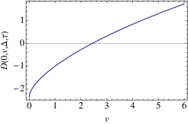
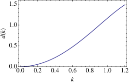
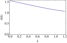
Figure 2: Continuum model with $R=1,\Delta=1,\tau^{2}=3.0$. (a) Graphical solution of equation (29b) yielding $v_{0}=2.4378>\Delta$. (b) $d(k)$ defined in Eq. (30), as function of $k$, showing $d(0)=0$ and $d^{\prime\prime}(0)>0$ namely $d(k)\approx Ck^{2}$ for small $k$ where $C=(1/2)d^{\prime\prime}(0)>0$. (c) Phase shift $\delta(k)$ as function $k$. The fact that $\delta(0)=\pi/2$, indicates a FR at threshold. Note that $4\Delta R^{2}=4<\pi^{2}$, namely, the closed channel (when uncoupled) does not have a bound-state. And yet, there is a FR in the coupled systems.

I.2 Bound-States of the Coupled System

Next we consider the bound-state in the continuum model specified by Eqs. (20) and (21) and show that there are bound-states of the coupled system even if the closed channel potential is repulsive. To show this, we need to solve the coupled Schrödinger equations and find a negative energy eigenvalue and square integrable wave function,

$$-\frac{d^{2}}{dr^{2}}f(r)+\tau\delta(r-R)g(r)+[v_{c}(r)+q^{2}]f(r)=0,\ \ f(0)=0,\ \ \mbox{(Equation for the closed channel wave function)},$$

$$-\frac{d^{2}}{dr^{2}}g(r)+\tau\delta(r-R)f(r)+q^{2}g(r)=0,\ \ g(0)=0,\ \ \mbox{(Equation for the open channel wave function)},$$ (31)

where $-q^{2}=\varepsilon_{B}<0$ is the bound-state energy. Denoting

$$\kappa\equiv\sqrt{v+q^{2}}>0,\ \ \alpha\equiv\sqrt{u+q^{2}}\equiv\sqrt{v-\Delta+q^{2}}\ \ \mbox{(either positive or pure imaginary)},$$ (32)

We have

$$f(r)=\begin{cases}A_{f}e^{-\kappa r}\ \ (x>R)\\ B_{f}\sinh\alpha r\ \ (r<R),\end{cases},\ \ g(r)=\begin{cases}A_{g}e^{-qr}\ \ (x>R)\\ B_{g}\sinh qr\ \ (r<R),\end{cases}$$ (33)

Now we obtain four homogeneous equations for the components of the vector $X\equiv(A_{f},B_{f},B_{g},A_{g})$ of unknown coefficients by matching the wave function and its derivative at $r=R$,

$$-f^{\prime}(R^{+})+f^{\prime}(R^{-})+\tau g(R)=0\ \Rightarrow A_{f}\kappa e^{-\kappa R}+B_{f}\alpha\cosh\alpha R+\tau A_{g}e^{-qR}=0,$$ (34a)

$$f(R^{+})=f(R^{-})\ \Rightarrow A_{f}e^{-\kappa R}-B_{f}\sinh\alpha R=0,$$ (34b)

$$g(R^{+})=g(R^{-})\ \Rightarrow A_{g}e^{-qR}-B_{g}\sinh qR=0,$$ (34c)

$$-g^{\prime}(R^{+})+g^{\prime}(R^{-})+\tau f(R)=0\ \Rightarrow A_{g}qe^{-qR}+B_{g}q\cosh qR+\tau A_{f}e^{-\kappa R}=0.$$ (34d)

Writing this set of equations as ${\cal M}(q)X=0$ the matrix ${\cal M}(q)$ is given by,

$${\cal M}(q)=\begin{pmatrix}\kappa e^{-\kappa R}&\alpha\cosh\alpha R&0&\tau e^{-qR}\\ e^{-\kappa R}&-\sinh\alpha R&0&0\\ 0&0&-\sinh qR&e^{-qR}\\ \tau e^{-\kappa R}&0&q\cosh qR&qR^{-qR}.\end{pmatrix}$$ (35)

A zero of the determinant at $q_{B}>0$ indicates a bound-state of the coupled system with bound-state energy $\varepsilon_{B}=-q_{B}^{2}$. An example is given in Fig. 3.

Figure 3: Det$[{\cal M}(q)]$ as function of $q$, where ${\cal M}(q)$ is given in Eq. (35). The parameters used are $(v,u,\tau,a)=(4,4.2,3,1)$. Note that $v-u=-0.2$, so that the spherical well $v_{c}(r)$ of the closed channel is repulsive (it has negative “depth” $\Delta=v-u$). And yet, the coupled system has a bound-state at energy $E_{B}=-q_{B}^{2}$ where $q_{B}\approx 0.81$. Performing graphical evaluation of $v_{0}$ for the relevant parameters [as in Fig. 2(a)] we find that $v\ll v_{0}$, i.e., the bound-state occurs for $v<v_{0}$ as it should be.

II II. The model defined by Eq. (1): Singularity of the $T$ matrix

We now examine a general two coupled-channel $s$-wave scattering problem in a 3D continuous geometry in which the open and closed channel have only a continuous spectrum. Under these conditions we prove, that this striking result is not an artifact of the TB model or of any other specific model. For this purpose, it is convenient to use the language of formal scattering theory without resorting to a specific representation. Let ${\cal H}_{o}$ and ${\cal H}_{c}$ denote the Hilbert spaces for the open and closed channel respectively. The corresponding Hamiltonians, $H_{o}$ and $H_{c}$, act in ${\cal H}_{o}$ and ${\cal H}_{c}$, whereas the coupling term $w$ can be considered as a mapping from ${\cal H}_{o}$ to ${\cal H}_{c}$. For a given scattering energy $\varepsilon$, the corresponding Green’s functions are denoted as $G_{o}(\varepsilon)=(\varepsilon+i\eta-H_{o})^{-1}$ and $G_{c}(\varepsilon)=(\varepsilon+i\eta-H_{c})^{-1}$ where $\eta\to 0^{+}$ guarantees the proper outgoing asymptotic conditions of the scattering states in configuration space.

Starting from Eq. (1) of the main text and eliminating the closed channel component $u_{c}$ we obtain a single equation for the open channel component $u_{o}\in{\cal H}_{o}$ with an effective (energy dependent) potential $v_{\mathrm{eff}}$,

$$[H_{o}+v_{\mathrm{eff}}(\varepsilon)]u_{o}=\varepsilon u_{o},\quad v_{\mathrm{eff}}(\varepsilon)=w^{\dagger}G_{c}(\varepsilon)w.$$ (36)

The $T$ matrix associated with $v_{\mathrm{eff}}(\varepsilon)$ is,

$$T(\varepsilon)=v_{\mathrm{eff}}(\varepsilon)[1-G_{o}(\varepsilon)v_{\mathrm{eff}}(\varepsilon)]^{-1}.$$ (37)

To get the scattering length from the $T$ matrix we denote by $\{|k\rangle\}$ and $\{e_{k}\geq 0\}$ the set of eigenstates and eigenvalues belonging to the continuous spectrum of $H_{o}$ (recall that in general, $H_{o}$ may also have a discrete spectrum). By definition, the $s$-wave scattering length is given by,

$$a=-C\lim_{e_{k}\to 0}\langle k|T(e_{k})|k\rangle,$$ (38)

where $C>0$ is a kinematic constant. Accordingly, an infinite $|a|$, the hallmark of a FR, implies a singularity of the on-shell $T$ matrix element as $e_{k}\to 0$. Our goal of proving that there is a FR even when the closed channel does not have a bound-state will be achieved by verifying the existence of a singularity of the $T$ matrix.

Let us first inspect the case where the closed channel does have a bound-state $|B\rangle$ with binding energy $\varepsilon_{B}$. (Recall that $\varepsilon_{B}$ is tunable, e.g., by a magnetic field). The occurrence of FR is then dominated by this bound-state as discussed in Ref. CCT where it is assumed that $G_{c}(\varepsilon)=|B\rangle\langle B|/(\varepsilon-\varepsilon_{B})$. The singularity of $v_{\mathrm{eff}}(\varepsilon)$ at $\varepsilon=\varepsilon_{B}$ is slightly shifted upward in the $T$ matrix denominator due to virtual transitions to the open channel subspace (self energy). This is the reason that, usually, FR occurs at zero scattering energy $\varepsilon=0^{+}$ for $\varepsilon_{B}>0$ as discussed in the main text.

Now suppose that both $H_{c}$ and $H_{o}$ only have a continuous spectrum, $\{\epsilon_{p}\geq v_{c}(\infty)>0\}$ (eigenvalues of $H_{c}$) and, as already specified, $\{e_{k}\geq 0\}$ (eigenvalues of $H_{o}$). Our strategy is to show that for a given negative energy $\varepsilon$, the system can be tuned by varying the strength $t$ of the coupling $w$ to obtain a bound-state at that energy. In particular, for $\varepsilon=0^{-}$ (meaning infinitesimally smaller than 0) we can thereby obtain a zero-energy bound-state. Then we can employ the fact that by a small upward shift of $v_{c}$, a zero energy bound-state at $\varepsilon=0^{-}$ becomes a zero-energy FR at $\varepsilon=0^{+}$ (see the Jost function discussion in the main text).

In Eq. (37) for the $T$ matrix, it is evident that $v_{\mathrm{eff}}(\varepsilon)$ is regular as $\varepsilon\to 0^{\pm}$ because $\varepsilon$ is outside the spectrum of $H_{c}$ defined by $0\leq\epsilon_{p}\leq\infty$. Therefore, if there is a singularity of $\langle k|T(e_{k})|k\rangle$ leading to an infinite scattering length, or a singularity of $\langle k|T(\varepsilon=0^{-}))|k\rangle$ that corresponds to a zero-energy bound-state, it must be associated with the second factor of the $T$ matrix,

$$[1-Q(\varepsilon)]^{-1}\equiv[1-G_{o}(\varepsilon)v_{\mathrm{eff}}(\varepsilon)]^{-1}=[1-G_{o}(\varepsilon)w^{\dagger}G_{c}(\varepsilon)w].$$ (39)

Thus, we need to show that $[1-Q(\varepsilon=0^{-})]^{-1}$ can be tuned to singularity. For this purpose, it is sufficient to show that $Q(\varepsilon=0^{-})$ acting in ${\cal H}_{o}$ is positive definite, because then, the operator $[1-Q(\varepsilon=0^{-})]^{-1}$ can be tuned to be singular (by varying the strength $t$ of the coupling $w$), leading to a pole of $\langle k|T(\varepsilon))|k\rangle$ at $\varepsilon=0^{-}$.

Sine both $H_{o}$ and $H_{c}$ have a positive continuous spectrum, the negative energies $\varepsilon<0$ are outside the spectra of both $H_{o}$ and $H_{c}$. Hence, there is no need to add a small imaginary part $i\eta$ to the energy variable because the limit $\eta\to 0$ can be safely applied. In other words, for $\varepsilon<0$,

$$Q(\varepsilon)=(\varepsilon-H_{o})^{-1}w^{\dagger}(\varepsilon-H_{c})^{-1}w.$$ (40)

Consider the eigenvalue equation defined for $|\psi\rangle\in{\cal H}_{o}$,

$$Q(\varepsilon)|\psi\rangle=(H_{o}-\varepsilon)^{-1}w^{\dagger}(H_{c}-\varepsilon)^{-1}w|\psi\rangle=\lambda|\psi\rangle~{}.$$ (41)

(Note that the double sign changes in the resolvents compensate each other). We want to show that as $\varepsilon\to 0^{-}$, $\lambda>0$. Clearly, for a given $\varepsilon<0$, both denominators are positive definite. Therefore, the operators $(H_{o}-\varepsilon)^{-1/2}$ and $(H_{c}-\varepsilon)^{-1/2}$ are both Hermitian. Using the notation, $|\psi\rangle=(H_{o}-\varepsilon)^{-1/2}|\phi\rangle$ the eigenvalue problem becomes Hermitian, i.e.,

$$\underbrace{(H_{o}-\varepsilon)^{-1/2}w^{\dagger}(H_{c}-\varepsilon)^{-1/2}}_{A^{\dagger}}\underbrace{(H_{c}-\varepsilon)^{-1/2}w(H_{o}-\varepsilon)^{-1/2}}_{A}|\phi\rangle=\lambda|\phi\rangle~{}.$$ (42)

Moreover, the Hermitian operator acting on $|\phi\rangle$ has the form $A^{\dagger}A$ where $A=(H_{c}-\varepsilon)^{-1/2}w(H_{o}-\varepsilon)^{-1/2}$, therefore, it is positive definite and hence $\lambda>0$. Thus, we have established that the system can be tuned to have a zero-energy bound-state. By an infinitesimally small upward shift of $v_{c}$ this bound-state becomes a pole of the on-shell $T$ matrix $\langle k|T(e_{k})|k\rangle$ as $k\to 0$, namely, a FR.

III III. Relation between coupling strength $\tau$ and the sign of $a$ near unitarity

From Eq. (2) we see that Sign$[a]=-$Sign$[\delta(0)]$. To elucidate the sign of $\delta(0)$ let us return to Eq. (11) of the main text, $\tan\delta=N(k,\tau,v_{0},\Delta,\Lambda)/D(k,\tau,v_{0},\Delta,\Lambda)$ where $v_{0}$ is defined in Eq. (12). Since $N(k...)=C\sin k\ \ (C>0)$, the sign of $a$ is determined by the sign of $D(k...)$ as $k\to 0$. It is more convenient to express $D$ as function of $\varepsilon_{k}$ and inspect its sign as $\varepsilon_{k}\to-2$. Explicitly,

$$D(\varepsilon_{k},\tau,v_{0},\Delta,\Lambda)=\sqrt{(v_{0}-\varepsilon_{k})^{2}-4}+v_{0}-2\Delta+(\tau^{2}-1)\varepsilon_{k}$$

$$\quad+\tfrac{1}{2}\Lambda\varepsilon_{k}[(v_{0}-2\Delta)+\sqrt{(v_{0}-\varepsilon_{k})^{2}-4}-\varepsilon_{k}]~{},$$ (43)

where $v_{0}$, defined in Eq. (12) of the text is such that $D(-2,\tau,v_{0},\Delta,\Lambda)=0$. Expanding $D(\varepsilon_{k},\tau,v_{0},\Delta,\Lambda)$ near threshold $\varepsilon_{k}=-2$ and recalling that, by construction, $D(-2,\tau,v_{0},\Delta,\Lambda)=0$ we get,

$$D(\varepsilon_{k},\tau,v_{0},\Delta,\Lambda)\approx D^{\prime}(-2,\tau,v_{0},\Delta,\Lambda)(\varepsilon_{k}+2)=4D^{\prime}(-2,\tau,v_{0},\Delta,\Lambda)\sin^{2}\tfrac{k}{2}~{}.$$ (44)

This result shows that (1) the denominator of $\tan\delta(k)$ vanishes faster that its numerator $N(k...)=C\sin k$, as discussed after equation (12) of the text. (2) The sign of $\delta(0)$ is determined by the sign of $D^{\prime}(-2,\tau,v_{0},\Delta,\Lambda)$. For fixed $\Lambda$ and $\Delta$, the function $f(\tau)\equiv D^{\prime}(-2,\tau,v_{0},\Delta,\Lambda$ is a complicated function of $\tau$ (recall that $v_{0}$ as given by Eq. (12) of the text also depends on $\tau$). However, it is not difficult to check that $f(\tau)$ changes sign at some point $\tau_{0}$ such that ${\mathrm{Sign}}[f(\tau)]={\mathrm{Sign}}[\delta(0)]={\mathrm{Sign}}[(\tau-\tau_{0})]$. Thus we have,

$${\mathrm{Sign}}[a]=-{\mathrm{Sign}}[\delta(0)]=\begin{cases}+\ \ (\tau<\tau_{0})\\ -\ \ (\tau>\tau_{0})\end{cases}.$$ (45)

In actuality, $\tau_{0}$ is only weakly dependent on $\Delta$ and $\Lambda$.

References

(1) H. Feshbach, Ann. Phys. N. Y. 5, 357-390
(1958), ibid., 19, 287-313 (1962).
(2) E. Timmermans, P. Tommasini, M. Hussein, and A. Kerman,
Phys. Rep. 315, 199 230 (1999).
(3) T. Köhler, K. Goral and P. S. Julienne,
Rev. Mod. Phys. 78, 1311-1361 (2006).
(5) C. Chin, R. Grimm and P. S. Julienne,
Rev. Mod. Phys. 82, 1225 (2010).
(6)
S. Blatt, et al.,
Phys. Rev. Lett. 107, 073202 (2011).
(7)
K. M. Jones, E. Tiesinga, P. D. Lett, and P. S. Julienne,
Rev. Mod. Phys. 78, 483-535 (2006).
(8)
C. A. Regal, M. Greiner, and D. S. Jin,
Phys. Rev. Lett. 92, 040403 (2004).
(9)
Here we consider a 3D continuous model. No periodic structure is
present as in
M. Olshanii, Phys. Rev. Lett. 81, 000938 (1998), and N.
Nygaard, R. Piil, and K. Molmer, Phys. Rev. A77, 021601(R)
(2008), who study FR in optical lattices in reduced dimension.
(11)
In a future publication, T. Wasak M. Trippenbach, Y. Avishai and Y. B.
Band, “Simple Feshbach Resonance Models”, (to be submitted), we
consider the case where more than one bound state occurs.
(12)
M. Valiente and D. Petrosyan, J. Phys. B41, 161002 (2008).
(13) R. G. Thomas, Phys. Rev. 88, 1109
(1952); J. B. Ehrman, Phys. Rev. 81, 412 (1951).
(14) J. R. Taylor, Scattering Theory: The Quantum
Theory on Nonrelativistic Collisions, (John Wiley & Sons, 1972),
Chp. 13 and Fig. 13.5; Y. B. Band and Y. Avishai, Quantum Mechanics, with Applications to Nanotechnology and Quantum
Information Science, (Elsevier, 2013), Secs. 12.5
and 12.6, and Fig. 12.9.
(15) Y. Castin and F. Werner, arXiv:1103.2851.
Supplementary Material for “Feshbach
Resonance without a Closed Channel Bound-State”

References

(1)
M. L. Godberger and K. M. Watson, Collision Theory, (Wiley, 1967),
p. 285.
(2) L. Ballentine, Quantum Mechanics, (World Scientific,
2000), p. 462.
(3) Y. B. Band and Y. Avishai Quantum Mechanics with Application
to Nanotechnology and Information Science, (Academic Press, 2013), p. 658.