Nonlinearity in oscillating bridges

Abstract

We first recall several historical oscillating bridges that, in some cases, led to collapses. Some of them are quite recent and show that, nowadays, oscillations in suspension bridges are not yet well understood. Next, we survey some attempts to model bridges with differential equations. Although these equations arise from quite different scientific communities, they display some common features. One of them, which we believe to be incorrect, is the acceptance of the linear Hooke law in elasticity. This law should be used only in presence of small deviations from equilibrium, a situation which does not occur in strongly oscillating bridges. Then we discuss a couple of recent models whose solutions exhibit self-excited oscillations, the phenomenon visible in real bridges. This suggests a different point of view in modeling equations and gives a strong hint how to modify the existing models in order to obtain a reliable theory. The purpose of this paper is precisely to highlight the necessity of revisiting classical models, to introduce reliable models, and to indicate the steps we believe necessary to reach this target.

AMS Subject Classification 2010: 74B20, 35G31, 34C15, 74K10, 74K20.

1 Introduction

The story of bridges is full of many dramatic events, such as uncontrolled oscillations which, in some cases, led to collapses. To get into the problem, we invite the reader to have a look at the videos [113, 115, 116, 117]. These failures have to be attributed to the action of external forces, such as the wind or traffic loads, or to macroscopic mistakes in the projects. From a theoretical point of view, there is no satisfactory mathematical model which, up to nowadays, perfectly describes the complex behavior of bridges. And the lack of a reliable analytical model precludes precise studies both from numerical and engineering points of views.

The main purpose of the present paper is to show the necessity of revisiting existing models since they fail to describe the behavior of real bridges. We will explain which are the weaknesses of the so far considered equations and suggest some possible improvements according to the fundamental rules of classical mechanics. Only with some nonlinearity and with a sufficiently large number of degrees of freedom several behaviors may be modeled. We do not claim to have a perfect model, we just wish to indicate the way to reach it. Much more work is needed and we explain what we believe to be the next steps.

We first survey and discuss some historical events, we recall what is known in elasticity theory, and we describe in full detail the existing models. With this database at hand, our purpose is to analyse the oscillating behavior of certain bridges, to determine the causes of oscillations, and to give an explanation to the possible appearance of different kinds of oscillations, such as torsional oscillations. Due to the lateral sustaining cables, suspension bridges most emphasise these oscillations which, however, also appear in other kinds of bridges: for instance, light pedestrian bridges display similar behaviors even if their mechanical description is much simpler.

According to [49], chaos is a disordered and unpredictable behavior of solutions in a dynamical system. With this characterization, there is no doubt that chaos is somehow present in the disordered and unpredictable oscillations of bridges. From [49, Section 11.7] we recall a general principle (GP) of classical mechanics:

(GP) The minimal requirements for a system of first-order equations to exhibit chaos is that they be nonlinear and have at least three variables.

This principle suggests that

any model aiming to describe oscillating bridges should be nonlinear and with enough degrees of freedom.

Most of the mathematical models existing in literature fail to satisfy (GP) and, therefore, must be accordingly modified. We suggest possible modifications of the corresponding differential equations and we believe that, if solved, this would lead to a better understanding of the underlying phenomena and, perhaps, to several practical actions for the plans of future bridges, as well as remedial measures for existing structures. In particular, one of the major scopes of this paper is to convince the reader that linear theories are not suitable for the study of bridges oscillations whereas, although they are certainly too naive, some recent nonlinear models do display self-excited oscillations as visible in bridges.

In Section 2, we collect a number of historical events and observations about bridges, both suspended and not. A complete story of bridges is far beyond the scopes of the present paper and the choice of events is mainly motivated by the phenomena that they displayed. The description of the events is accompanied by comments of engineers and of witnesses, and by possible theoretical explanations of the observed phenomena. The described events are then used in order to figure out a common behavior of oscillating bridges; in particular, it appears that the requirements of (GP) must be satisfied. Recent events testify that the problems of controlling and forecasting bridges oscillations is still unsolved.

In Section 3, we discuss several equations appearing in literature as models for oscillating bridges. Most of them use in some point the well-known linear Hooke law (${\cal LHL}$ in the sequel) of elasticity. This is what we believe to be a major weakness, but not the only one, of all these models. This is also the opinion of McKenna [69, p.16]:

We doubt that a bridge oscillating up and down by about 10 meters every 4 seconds obeys Hooke’s law.

From [31], we recall what is known as ${\cal LHL}$.

The linear Hooke law (${\bf{\cal LHL}}$) of elasticity, discovered by the English scientist Robert Hooke in 1660, states that for relatively small deformations of an object, the displacement or size of the deformation is directly proportional to the deforming force or load. Under these conditions the object returns to its original shape and size upon removal of the load. … At relatively large values of applied force, the deformation of the elastic material is often larger than expected on the basis of ${\cal LHL}$, even though the material remains elastic and returns to its original shape and size after removal of the force. ${\cal LHL}$ describes the elastic properties of materials only in the range in which the force and displacement are proportional.

Hence, by no means one should use ${\cal LHL}$ in presence of large deformations. In such case, the restoring elastic force $f$ is “more than linear”. Instead of having the usual form $f(s)=ks$, where $s$ is the displacement from equilibrium and $k>0$ depends on the elasticity of the deformed material, it has an additional superlinear term $\varphi(s)$ which becomes negligible for small displacements $s$. More precisely,

$$f(s)=ks+\varphi(s)\qquad\mbox{with}\qquad\lim_{s\to 0}\frac{\varphi(s)}{s}=0\ .$$

The simplest example of such term is $\varphi(s)=\varepsilon s^{p}$ with $\varepsilon>0$ and $p>1$; this superlinear term may become arbitrarily small for $\varepsilon$ small and/or $p$ large. Therefore, the parameters $\varepsilon$ and $p$, which do exist, may be chosen in such a way to describe with a better precision the elastic behavior of a material when large displacements are involved. As we shall see, this apparently harmless and tiny nonlinear perturbation has devastative effects on the models and, moreover, it is amazingly useful to display self-excited oscillations as the ones visible in real bridges. On the contrary, linear models prevent to view the real phenomena which occur in bridges, such as the sudden increase of the width of their oscillations and the switch to different ones.

The necessity of dealing with nonlinear models is by now quite clear also in more general elasticity problems; from the preface of the book by Ciarlet [23], let us quote

… it has been increasingly acknowledged that the classical linear equations of elasticity, whose mathematical theory is now firmly established, have a limited range of applicability, outside of which they should be replaced by genuine nonlinear equations that they in effect approximate.

In order to model bridges, the most natural way is to view the roadway as a thin narrow rectangular plate. In Section 3.1, we quote several references which show that classical linear elastic models for thin plates do not describe with a sufficient accuracy large deflections of a plate. But even linear theories present considerable difficulties and a further possibility is to view the bridge as a one dimensional beam; this model is much simpler but, of course, it prevents the appearance of possible torsional oscillations. This is the main difficulty in modeling bridges: find simple models which, however, display the same phenomenon visible in real bridges.

In Section 3.2 we survey a number of equations arising from different scientific communities. The first equations are based on engineering models and mainly focus the attention on quantitative aspects such as the exact values of the parameters involved. Some other equations are more related to physical models and aim to describe in full details all the energies involved. Finally, some of the equations are purely mathematical models aiming to reach a prototype equation and proving some qualitative behavior. All these models have to face a delicate choice: either consider uncoupled behaviors between vertical and torsional oscillations of the roadway or simplify the model by decoupling these two phenomena. In the former case, the equations have many degrees of freedom and become terribly complicated: hence, very few results can be obtained. In the latter case, the model fails to satisfy the requirements of (GP) and appears too far from the real world.

As a compromise between these two choices, in Section 4 we recall the model introduced in [46, 48] which describes vertical oscillations and torsional oscillations of the roadway within the same simplified beam equation. The solution to the equation exhibits self-excited oscillations quite similar to those observed in suspension bridges. We do not believe that the simple equation considered models the complex behavior of bridges but we do believe that it displays the same phenomena as in more complicated models closer related to bridges. In particular, finite time blow up occurs with wide oscillations. These phenomena are typical of differential equations of at least fourth order since they do not occur in lower order equations, see [46]. We also show that the same phenomenon is visible in a $2\times 2$ system of nonlinear ODE’s of second order related to a system suggested by McKenna [69].

Putting all together, in Section 5 we afford an explanation in terms of the energies involved. Starting from a survey of milestone historical sources [14, 98], we attempt a qualitative but detailed energy balance and we attribute the appearance of torsional oscillations in bridges to some “hidden” elastic energy which is not visible since it involves second order derivatives of the displacement of the bridge: this suggests an analogy between bridges oscillations and a ball bouncing on the floor. The discovery of the phenomenon usually called in literature flutter speed has to be attributed to Bleich [13]; in our opinion, the flutter speed should be seen as a critical energy threshold which, if exceeded, gives rise to uncontrolled phenomena such as torsional oscillations. We give some hints on how to determine the critical energy threshold, according to some eigenvalue problems whose eigenfunctions describe the oscillating modes of the roadway.

In bridges one should always expect vertical oscillations and, in case they become very large, also torsional oscillations; in order to display the possible transition between these two kinds of oscillations, in Section 6.1 we suggest a new equation as a model for suspension bridges, see (54). With all the results and observations at hand, in Section 6.2 we also attempt a detailed description of what happened on November 10, 1940, the day when the Tacoma Narrows Bridge collapsed. As far as we are aware a universally accepted explanation of this collapse in not yet available. Our explanation fits with all the material developed in the present paper. This allows us to suggest a couple of precautions when planning future bridges, see Section 6.3.

We recently had the pleasure to participate to a conference on bridge maintenance, safety and management, see [55]. There were engineers from all over the world, the atmosphere was very enjoyable and the problems discussed were extremely interesting. And there was a large number of basic questions still unsolved, most of the results and projects had some percentage of incertitude. Many talks were devoted to suggest new equations to model the studied phenomena and to forecast the impact of new structural issues: even apparently simple problems are still unsolved. We believe this should be a strong motivation for many mathematicians (from mathematical physics, analysis, numerics) to get interested in bridges modeling, experiments, and performances. Throughout the paper we suggest a number of open problems which, if solved, could be a good starting point to reach a deeper understanding of oscillations in bridges.

2 What has been observed in bridges

A simplified picture of a suspension bridge can be sketched as in Figure 1

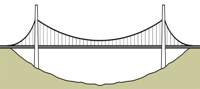
Figure 1: Suspension bridges without girder and with girder.

where one sees the difference between the elastic structure of a bridge without girder and the more stiff structure of a bridge with girder.

Although the first project of a suspension bridge is due to the Italian engineer Verantius around 1615, see [104] and [81, p.7] or [57, p.16], the first suspension bridges were built only about two centuries later in Great Britain. According to [11],

The invention of the suspension bridges by Sir Samuel Brown sprung from the sight of a spider’s web hanging across the path of the inventor, observed on a morning’s walk, when his mind was occupied with the idea of bridging the Tweed.

Samuel Brown (1776-1852) was an early pioneer of suspension bridge design and construction. He is best known for the Union Bridge of 1820, the first vehicular suspension bridge in Britain.

An event deserving mention is certainly the inauguration of the Menai Straits Bridge, in 1826. The project of the bridge was due to Thomas Telford and the opening of the bridge is considered as the beginning of a new science nowadays known as “Structural Engineering”. The construction of this bridge had a huge impact in the English society, a group of engineers founded the “Institution of Civil Engineers” and Telford was elected the first president of this association. In 1839 the Menai Bridge collapsed due to a hurricane. In that occasion, unexpected oscillations appeared; Provis [86] provided the following description:

… the character of the motion of the platform was not that of a simple undulation, as had been anticipated, but the movement of the undulatory wave was oblique, both with respect to the lines of the bearers, and to the general direction of the bridge.

Also the Broughton Suspension Bridge was built in 1826. It collapsed in 1831 due to mechanical resonance induced by troops marching over the bridge in step. A bolt in one of the stay-chains snapped, causing the bridge to collapse at one end, throwing about 40 men into the river. As a consequence of the incident, the British Army issued an order that troops should “break step” when crossing a bridge. These two pioneering bridges already show how the wind and/or traffic loads, both vehicles and pedestrians, play a crucial negative role in the bridge stability.

A further event deserving to be mentioned is the collapse of the Brighton Chain Pier, built in 1823. It collapsed a first time in 1833, it was rebuilt and partially destroyed once again in 1836. Both the collapses are attributed to violent windstorms. For the second collapse a witness, William Reid, reported valuable observations and sketched a picture illustrating the destruction [87, p.99], see Figure 2

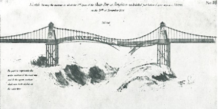
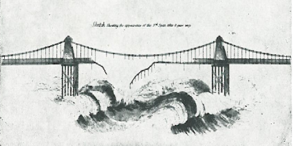
Figure 2: Destruction of the Brighton Chain Pier.

which is taken from [90]. This is the first reliable report on oscillations appearing in bridges, the most intriguing part of the report being [87, 90]:

For a considerable time, the undulations of all the spans seemed nearly equal … but soon after midday the lateral oscillations of the third span increased to a degree to make it doubtful whether the work could withstand the storm; and soon afterwards the oscillating motion across the roadway, seemed to the eye to be lost in the undulating one, which in the third span was much greater than in the other three; the undulatory motion which was along the length of the road is that which is shown in the first sketch; but there was also an oscillating motion of the great chains across the work, though the one seemed to destroy the other …

More comments about this collapse are due to Russell [91]; in particular, he claims that

… the remedies I have proposed, are those by which such destructive vibrations would have been rendered impossible.

These two comments may have several interpretations. However, what appears absolutely clear is that different kinds of oscillations appeared (undulations, lateral oscillations, oscillation motion of the great chains) and some of them were considered destructive. Further details on the Brighton Chair Pier collapse may be found in [14, pp.4-5].

Some decades earlier, at the end of the eighteenth century, the German physicist Ernst Chladni was touring Europe and showing, among other things, the nodal line patterns of vibrating plates, see Figure 3.

Figure 3: Chladni patterns in a vibrating plate.

Chladni’s technique, first published in [22], consisted of creating vibrations in a square-shaped metal plate whose surface was covered with light sand. The plate was bowed until it reached resonance, when the vibration caused the sand to concentrate along the nodal lines of vibrations, see [114] for the nowadays experiment. This simple but very effective way to display the nodal lines of vibrations was seen by Navier [80] as

Les curieuses expériences de M. Chaldni sur les vibrations des plaques…

It appears quite clearly from Figure 3 how complicated may be the vibrations of a thin plate and hence, see Section 3.1, of a bridge. And, indeed, the just described events testify that, besides the somehow expected vertical oscillations, also different kinds of oscillations may appear. For instance, one may have “an oblique undulatory wave” or some kind of resonance or the interaction with other structural components such as the suspension chains. The description of different coexisting forms of oscillations is probably the most important open problem in suspension bridges.

It is not among the scopes of this paper to give the complete story of bridges collapses for which we refer to [14, Section 1.1], to [90, Chapter IV], to [24, 34, 54, 109], to the recent monographs [3, 57], and also to [56] for a complete database. Let us just mention that between 1818 and 1889, ten suspension bridges suffered major damages or collapsed in windstorms, see [34, Table 1, p.13], which is commented by

An examination of the British press for the 18 years between 1821 and 1839 shows it to be more replete with disastrous news of suspension bridges troubles than Table 1 reveals, since some of these structures suffered from the wind several times during this period and a number of other suspension bridges were damaged or destroyed as a result of overloading.

The story of bridges, suspended and not, contains many further dramatic events, an amazing amount of bridges had troubles for different reasons such as the wind, the traffic loads, or macroscopic mistakes in the project, see e.g. [53, 83]. Among them, the most celebrated is certainly the Tacoma Narrows Bridge, collapsed in 1940 just a few months after its opening, both because of the impressive video [116] and because of the large number of studies that it has inspired starting from the reports [5, 14, 34, 35, 36, 98, 106].

Let us recall some observations made on the Tacoma collapse. Since we were unable to find the Federal Report [5] that we repeatedly quote below, we refer to it by trusting the valuable historical research by Scott [97] and by McKenna and coauthors, see in particular [63, 69, 70, 74]. A good starting point to describe the Tacoma collapse is… the Golden Gate Bridge, inaugurated a few years earlier, in 1937. This bridge is usually classified as “very flexible” although it is strongly stiffened by a thick girder, see Figure 4.

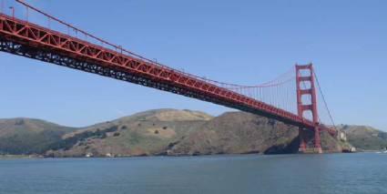
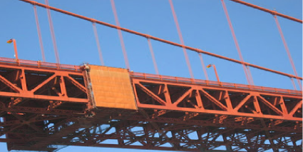
Figure 4: Girder at the Golden Gate Bridge.

The original roadway was heavy and made with concrete; the weight was reduced in 1986 when a new roadway was installed, see [85]. Nowadays, in spite of the girder, the bridge can swing more than an amazing 8 meters and flex about 3 meters under big loads, which explains why the bridge is classified as very flexible. The huge mass involved and these large distances from equilibrium explain why ${\cal LHL}$ certainly fails. Due to high winds around 120 kilometers per hour, the Golden Gate Bridge has been closed, without suffering structural damage, only three times: in 1951, 1982, 1983, always during the month of December. A further interesting phenomenon is the appearance of traveling waves in 1938: in [5, Appendix IX] (see also [74]), the chief engineer of the Golden Gate Bridge writes

… I observed that the suspended structure of the bridge was undulating vertically in a wavelike motion of considerable amplitude …

see also the related detailed description in [74, Section 1]. Hence, one should also expect traveling waves in bridges, see the sketched representation in the first picture in Figure 5.

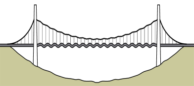
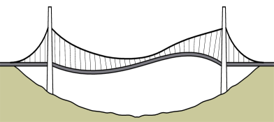
Figure 5: Traveling waves and torsional motion in bridges without girder.

All this may occur also in apparently stiff structures. And in presence of extremely flexible structures, these traveling waves can generate further dangerous phenomena such as torsional oscillations, see the second picture in Figure 5.

When comparing the structure of the Golden Gate Bridge with the one of the original Tacoma Narrows Bridge, one immediately sees a main macroscopic difference: the thick girder sustaining the bridge, compare Figures 4 and 6. The girder gives more stiffness to the bridge; this is certainly the main reason why in the Golden Gate Bridge no torsional oscillation ever appeared. A further reason is that larger widths of the roadway seem to prevent torsional oscillations, see (36) below; from [90, p.186] we quote

… a bridge twice as wide will have exactly double the critical speed wind.

The Tacoma Bridge was rebuilt with a thick girder acting as a strong stiffening structure, see [36]: as mentioned by Scanlan [95, p.840],

the original bridge was torsionally weak, while the replacement was torsionally stiff.

The replacement of the original bridge opened in 1950, see [36] for some remarks on the project, and still stands today as the westbound lanes of the present-day twin bridge complex, the eastbound lanes opened in 2007. Figure 6 - picture by Michael Goff, Oregon Department of Transportation, USA - shows the striking difference between the original Tacoma Bridge collapsed in 1940 and the twin bridges as they are today.

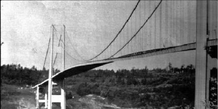
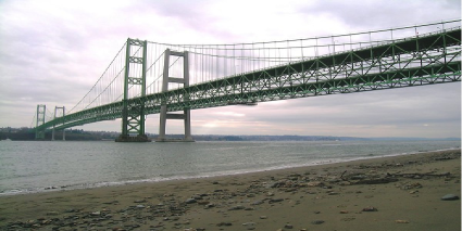
Figure 6: The collapsed Tacoma Bridge and the current twins Tacoma Bridges.

Let us go back to the original Tacoma Bridge: even if it was extremely flexible, it is not clear why torsional oscillations appeared. According to Scanlan [95, p.841],

… some of the writings of von Kármán leave a trail of confusion on this point. … it can clearly be shown that the rhythm of the failure (torsion) mode has nothing to do with the natural rhythm of shed vortices following the Kármán vortex street pattern. … Others have added to the confusion. A recent mathematics text, for example, seeking an application for a developed theory of parametric resonance, attempts to explain the Tacoma Narrows failure through this phenomenon.

Hence, Scanlan discards the possibility of the appearance of von Kármán vortices and raises doubts on the appearance of resonance which, indeed, is by now also discarded. Of course, it is reasonable to expect resonance in presence of a single-mode solicitation, such as for the Broughton Bridge. But for the Tacoma Bridge, Lazer-McKenna [63, Section 1] raise the question

… the phenomenon of linear resonance is very precise. Could it really be that such precise conditions existed in the middle of the Tacoma Narrows, in an extremely powerful storm?

So, no plausible explanation is available nowadays. In a letter [33], Prof. Farquharson claimed that

… a violent change in the motion was noted. This change appeared to take place without any intermediate stages and with such extreme violence … The motion, which a moment before had involved nine or ten waves, had shifted to two.

All this happened under not extremely strong winds, about 80km/h, and under a relatively high frequency of oscillation, about 36cpm, see [34, p.23]. See [69, Section 2.3] for more details and for the conclusion that

there is no consensus on what caused the sudden change to torsional motion.

This is confirmed by the following ambiguous comments taken from [14, Appendix D]:

If vertical and torsional oscillations occur, they must be caused by vertical components of wind forces or by some structural action which derives vertical reactions from a horizontally acting wind.

This part is continued in [14] by stating that there exist references to both alternatives and that

A few instrumental measurements have been made … which showed the wind varying up to 8 degrees from the horizontal. Such variation from the horizontal is not the only, and perhaps not the principal source of vertical wind force on a structure.

Besides the lack of consensus on the causes of the switch between vertical and torsional oscillations, all the above comments highlight a strong instability of the oscillation motion as if, after reaching some critical energy threshold, an impulse (a Dirac delta) generated a new unexpected motion. Refer to Section 6 for our own interpretation of this phenomenon which is described in [5, 14] (see also [97, pp.50-51]) as:

large vertical oscillations can rapidly change, almost instantaneously, to a torsional oscillation.

We do not completely agree with this description since a careful look at [116] shows that vertical oscillations continue also after the appearance of torsional oscillations; in the video, one sees that at the beginning of the bridge the street-lamps oscillate in opposition of phase when compared with the street-lamps at the end of the bridge. So, the phenomenon which occurs may be better described as follows:

large vertical oscillations can rapidly create, almost instantaneously, additional torsional oscillations.

Roughly speaking, we believe that part of the energy responsible of vertical oscillations switches to another energy which generates torsional oscillations; the switch occurs without intermediate stages as if an impulse was responsible of it. Our own explanation to this fact is that

since vertical oscillations cannot be continued too far downwards below the equilibrium position due to the hangers, when the bridge reaches some limit horizontal position with large kinetic energy, part of the energy transforms into elastic energy and generates a crossing wave, namely a torsional oscillation.

We make this explanation more precise in Section 5.2, after some further observations. In order to explain the “switch of oscillations” several mathematical models were suggested in literature. In next section we survey some of these models which are quite different from each other although they have some common features.

The Deer Isle Bridge, see Figure 7,

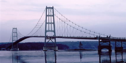
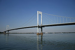
Figure 7: The Deer Isle Bridge (left) and the Bronx-Whitestone Bridge (right).

is a suspension bridge in the state of Maine (USA) which encountered wind stability problems similar to those of the original Tacoma Bridge. Before the bridge was finished, in 1939, the wind induced motion in the relatively lightweight roadway. Diagonal stays running from the sustaining cables to the stiffening girders on both towers were added to stabilize the bridge. Nevertheless, the oscillations of the roadway during some windstorms in 1942 caused extensive damage and destroyed some of the stays. At that time everybody had the collapse of the Tacoma Bridge in mind, so that stronger and more extensive longitudinal and transverse diagonal stays were added. In her report [77], Barbara Moran wrote

The Deer Isle Bridge was built at the same time as the Tacoma Narrows, and with virtually the same design. One difference: it still stands.

This shows strong instability: even if two bridges are considered similar they can react differently to external solicitations. Of course, much depends on what is meant by “virtually similar”…

The Bronx-Whitestone Bridge displayed in Figure 7, was built in New York in 1939 and has shown an intermitted tendency to mild vertical motion from the time the floor system was installed. The reported motions have never been very large, but were noticeable to the traveling public. Several successive steps were taken to stabilise the structure, see [6]. Midspan diagonal stays and friction dampers at the towers were first installed; these were later supplemented by diagonal stayropes from the tower tops to the roadway level. However, even these devices were not entirely adequate and in 1946 the roadway was stiffened by the addition of truss members mounted above the original plate girders, the latter becoming the lower chords of the trusses [4, 82]. This is a typical example of bridge built without considering all the possible external effects, subsequently damped by means of several unnatural additional components. Our own criticism is that

instead of just solving the problem, one should understand the problem.

And precisely in order to understand the problem, we described above those events which displayed the pure elastic behavior of bridges. These were mostly suspension bridges without girders and were free to oscillate. This is a good reason why the Tacoma collapse should be further studied for deeper knowledge: it displays the pure motion without stiffening constraints which hide the elastic features of bridges.

The Tacoma Bridge collapse is just the most celebrated and dramatic evidence of oscillating bridge but bridges oscillations are still not well understood nowadays. On May 2010, the Russian authorities closed the Volgograd Bridge to all motor traffic due to its strong vertical oscillations (traveling waves) caused by windy conditions, see [117] for the BBC report and video. Once more, these oscillations may appear surprising since the Volgograd Bridge is a concrete girder bridge and its stiffness should prevent oscillations. However, it seems that strong water currents in the Volga river loosened one of the bridge’s vertical supports so that the stiffening effect due to the concrete support was lost and the behavior became more similar to that of a suspension bridge. The bridge remained closed while it was inspected for damage. As soon as the original effect was restored the bridge reopened for public access. In Figure 8 the reader finds pictures of the bridge and of the damped sustaining support.

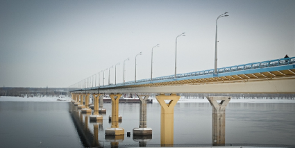
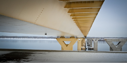
Figure 8: The Volgograd Bridge.

These pictures are taken from [32], where one can also find full details on the damping system of the bridge. The Volgograd Bridge well shows how oscillation induced fatigue of the structural members of bridges is a major factor limiting the life of the bridge. In [58] one may find a mathematical analysis and wind tunnel tests for examining oscillations which occur under “constant low wind”, rather than under violent windstorms:

Limited oscillation could even cause a collapse of light suspension bridges in a reasonably short time.

As already observed, the wind is not the only possible external source which generates bridges oscillations which also appear in pedestrian bridges where lateral swaying is the counterpart of torsional oscillation. In June 2000, the very same day when the London Millennium Bridge opened and the crowd streamed on it, the bridge started to sway from side to side, see [115]. Many pedestrians fell spontaneously into step with the vibrations, thereby amplifying them. According to Sanderson [92], the bridge wobble was due to the way people balanced themselves, rather than the timing of their steps. Therefore, the pedestrians acted as negative dampers, adding energy to the bridge’s natural sway. Macdonald [66, p.1056] explains this phenomenon by writing

… above a certain critical number of pedestrians, this negative damping overcomes the positive structural damping, causing the onset of exponentially increasing vibrations.

Although we have some doubts about the real meaning of “exponentially increasing vibrations” we have no doubts that this description corresponds to a superlinear behavior which has also been observed in several further pedestrian bridges, see [41] and [112] from which we quote

… damping usually increases with increasing vibration magnitude due to engagement of additional damping mechanisms.

The Millennium Bridge was made secure by adding some stiffening trusses below the girder, see Figure 9 (Photo $\copyright$ Peter Visontay).

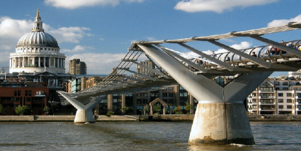
Figure 9: The London Millennium Bridge.

The mathematical explanation of this solution is that trusses lessen swaying and force the bridge to remain closer to its equilibrium position, that is, closer to a linear behavior as described by ${\cal LHL}$. Although trusses delay the appearance of the superlinear behavior, they do not solve completely the problem as one may wonder what would happen if 10.000 elephants would simultaneously walk through the Millennium Bridge… In this respect, let us quote from [34, p.13] a comment on suspension bridges strengthened by stiffening girders:

That significant motions have not been recorded on most of these bridges is conceivably due to the fact that they have never been subjected to optimum winds for a sufficient period of time.

Another pedestrian bridge, the Assago Bridge in Milan (310m long), had a similar problem. In February 2011, just after a concert the publics crossed the bridge and, suddenly, swaying became so violent that people could hardly stand, see [37] and [113]. Even worse was the subsequent panic effect when the crowd started running in order to escape from a possible collapse; this amplified swaying but, quite luckily, nobody was injured. In this case, the project did not take into account that a large number of people would go through the bridge just after the events; when swaying started there were about 1.200 pedestrians on the footbridge. This problem was solved by adding positive dampers, see [99].

According to [56], around 400 recorded bridges failed for several different reasons and the ones who failed after year 2000 are more than 70. Probably, some years after publication of this paper, these numbers will have increased considerably… The database [56] consists mainly of brief descriptions and statistics for each bridge failure: location, number of fatalities/injuries, etc. rather than in-depth analysis of the cause of the failure for which we refer to the nice book by Akesson [3].

As we have seen, the reasons of failures are of different kinds. Firstly, strong and/or continued winds: these may cause wide vertical oscillations which may switch to different kinds of oscillations. Especially for suspension bridges the latter phenomenon appears quite evident, due to the many elastic components (cables, hangers, towers, etc.) which appear in it. A second cause are traffic loads, such as some precise resonance phenomenon, or some unpredictable synchronised behavior, or some unexpected huge load; these problems are quite common in many different kinds of bridges. Finally, a third cause are mistakes in the project; these are both theoretical, for instance assuming ${\cal LHL}$, and practical, such as wrong assumptions on the possible maximum external actions.

After describing so many disasters, we suggest a joke which may sound as a provocation. Since many bridges projects did not forecast oscillations it could be more safe to build old-fashioned rock bridges, such as the Roman aqueduct built in Segovia (Spain) during the first century and still in perfect shape and in use. Of course, we are not suggesting here to replace the Golden Gate Bridge with a Roman-style bridge! But we do suggest to plan bridges by taking into account all possible kinds of solicitations. Moreover, we suggest not to hide unsolved problems with some unnatural solutions such as stiff and heavy girders or more extensive longitudinal and transverse diagonal stays, see Section 6.3 for more suggestions.

Throughout this section we listed a number of historical events about bridges. They taught us the following facts:

1. Self-excited oscillations appear in bridges. Often this is somehow unexpected since the project does not take into account several external strong and/or prolonged effects. And even if expected, oscillations can be much wider than estimated.

2. Oscillations can be extenuated by stiffening the structure or by adding positive (and heavy, and expensive) dampers to the structure. However, none of these solutions can completely prevent oscillations, especially in presence of highly unfavorable events such as strong and prolonged winds, not necessarily hurricanes, or heavy and synchronised traffic loads. Due to the unnatural stiffness of the structure, trusses and dampers may cause cracks, see [110] and references therein; but we leave this problem to engineers… see [57].

3. The oscillations are amplified by an observable superlinear effect. More the bridge is far from its equilibrium position, more the impact of external forces is relevant. It is by now well understood that suspension bridges behave nonlinearly, see e.g. [16, 60].

4. In extremely flexible bridges, such as the Tacoma Bridge which had no stiffening truss, vertical oscillations can partially switch to torsional oscillations and even to more complicated oscillations, see the pictures in Figure 10 which are taken from [108, p.143]

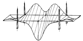
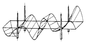
Figure 10: Combined oscillations of a bridge roadway.

and see also [90, pp.94-95] and Figure 11 below. This occurs when vertical oscillations become too large and, in such case, vertical and torsional oscillations coexist. Up to nowadays, there is no convincing explanation why the switch occurs.

3 How to model bridges

The amazing number of failures described in the previous section shows that the existing theories and models are not adequate to describe the statics and the dynamics of oscillating bridges. In this section we survey different points of view, different models, and we underline their main weaknesses. We also suggest how to modify them in order to fulfill the requirements of (GP).

3.1 A quick overview on elasticity: from linear to semilinear models

A quite natural way to describe the bridge roadway is to view it as a thin rectangular plate. This is also the opinion of Rocard [90, p.150]:

The plate as a model is perfectly correct and corresponds mechanically to a vibrating suspension bridge…

In this case, a commonly adopted theory is the linear one by Kirchhoff-Love [59, 65], see also [45, Section 1.1.2], which we briefly recall. The bending energy of a plate involves curvatures of the surface. Let $\kappa_{1}$, $\kappa_{2}$ denote the principal curvatures of the graph of a smooth function $u$ representing the deformation of the plate, then a simple model for the bending energy of the deformed plate $\Omega$ is

$$\mathbb{E}(u)=\int_{\Omega}\left(\frac{\kappa_{1}^{2}}{2}+\frac{\kappa_{2}^{2}}{2}+\sigma\kappa_{1}\kappa_{2}\right)\,dx_{1}dx_{2}$$ (1)

where $\sigma$ denotes the Poisson ratio defined by $\sigma=\frac{\lambda}{2\left(\lambda+\mu\right)}$ with the so-called Lamé constants $\lambda,\mu$ that depend on the material. For physical reasons it holds that $\mu>0$ and usually $\lambda\geq 0$ so that $0\leq\sigma<\frac{1}{2}$. In the linear theory of elastic plates, for small deformations $u$ the terms in (1) are considered to be purely quadratic with respect to the second order derivatives of $u$. More precisely, for small deformations $u$, one has

$$(\kappa_{1}+\kappa_{2})^{2}\approx(\Delta u)^{2}\ ,\quad\kappa_{1}\kappa_{2}\approx\det(D^{2}u)=(u_{x_{1}x_{1}}u_{x_{2}x_{2}}-u_{x_{1}x_{2}}^{2})\ ,$$

and therefore

$$\frac{\kappa_{1}^{2}}{2}+\frac{\kappa_{2}^{2}}{2}+\sigma\kappa_{1}\kappa_{2}\approx\frac{1}{2}(\Delta u)^{2}+(\sigma-1)\det(D^{2}u).$$

Then (1) yields

$$\mathbb{E}(u)=\int_{\Omega}\left(\frac{1}{2}\left(\Delta u\right)^{2}+(\sigma-1)\det(D^{2}u)\right)\,dx_{1}dx_{2}\,.$$ (2)

Note that for $-1<\sigma<1$ the functional $\mathbb{E}$ is coercive and convex. This modern variational formulation appears in [42], while a discussion for a boundary value problem for a thin elastic plate in a somehow old fashioned notation is made by Kirchhoff [59]. And precisely the choice of the boundary conditions is quite delicate since it depends on the physical model considered.

Destuynder-Salaun [28, Section I.2] describe this modeling by

… Kirchhoff and Love have suggested to assimilate the plate to a collection of small pieces, each one being articulated with respect to the other and having a rigid-body behavior. It looks like these articulated wooden snakes that children have as toys. Hence the transverse shear strain remains zero, while the planar deformation is due to the articulation between small blocks. But this simplified description of a plate movement can be acceptable only if the components of the stress field can be considered to be negligible.

The above comment says that ${\cal LHL}$ should not be adopted if the components of the stress field are not negligible. An attempt to deal with large deflections for thin plates is made by Mansfield [67, Chapters 8-9]. He first considers approximate methods, then with three classes of asymptotic plate theories: membrane theory, tension field theory, inextensional theory. Roughly speaking, the three theories may be adopted according to the ratio between the thickness of the plate and the typical planar dimension: for the first two theories the ratio should be less than $10^{-3}$, whereas for the third theory it should be less than $10^{-2}$. Since a roadway has a length of the order of 1km, the width of the order of 10m, even for the less stringent inextensional theory the thickness of the roadway should be less than 10cm which, of course, appears unreasonable. Once more, this means that ${\cal LHL}$ should not be adopted in bridges. In any case, Mansfield [67, p.183] writes

The exact large-deflection analysis of plates generally presents considerable difficulties…

Destuynder-Salaun [28, Section I.2] also revisit an alternative model due to Naghdi [79] by using a mixed variational formulation. They refer to [76, 88, 89] for further details and modifications, and conclude by saying that none between the Kirchhoff-Love model or one of these alternative models is always better than the others. Moreover, also the definition of the transverse shear energy is not universally accepted: from [28, p.149], we quote

… this discussion has been at the origin of a very large number of papers from both mathematicians and engineers. But to our best knowledge, a convincing justification concerning which one of the two expressions is the more suitable for numerical purpose, has never been formulated in a convincing manner. This question is nevertheless a fundamental one …

It is clear that a crucial role is played by the word “thin”. What is a thin plate? Which width is it allowed to have? If we assume that the width is zero, a quite unrealistic assumption for bridges, a celebrated two-dimensional equation was suggested by von Kármán [107]. This equation has been widely, and satisfactorily, studied from several mathematical points of view such as existence, regularity, eigenvalue problems, semilinear versions, see e.g. [45] for a survey of results. On the other hand, quite often several doubts have been raised on their physical soundness. For instance, Truesdell [102, pp.601-602] writes

Being unable to explain just why the von Kármán theory has always made me feel a little nauseated as well as very slow and stupid, I asked an expert, Mr. Antman, what was wrong with it. I can do no better than paraphrase what he told me: it relies upon

1) “approximate geometry”, the validity of which is assessable only in terms of some other theory.

2) assumptions about the way the stress varies over a cross-section, assumptions that could be justified only in terms of some other theory.

3) commitment to some specific linear constitutive relation - linear, that is, in some special measure of strain, while such approximate linearity should be outcome, not the basis, of a theory.

4) neglect of some components of strain - again, something that should be proved mathematically from an overriding, self-consistent theory.

5) an apparent confusion of the referential and spatial descriptions - a confusion that is easily justified for the classical linearised elasticity but here is carried over unquestioned, in contrast with all recent studies of the elasticity of finite deformations.

Truesdell then concludes with a quite eloquent comment:

These objections do not prove that anything is wrong with von Kármán strange theory. They merely suggest that it would be difficult to prove that there is anything right about it.

Let us invite the interested reader to have a careful look at the paper by Truesdell [102]; it contains several criticisms exposed in a highly ironic and exhilarating fashion and, hence, very effective.

Classical books for elasticity theory are due to Love [65], Timoshenko [100], Ciarlet [23], Villaggio [105], see also [78, 79, 101] for the theory of plates. Let us also point out a celebrated work by Ball [9] who was the first analyst to approach the real 3D boundary value problems for nonlinear elasticity. Further nice attempts to tackle nonlinear elasticity in particular situations were done by Antman [7, 8] who, however, appears quite skeptic on the possibility to have a general theory:

… general three-dimensional nonlinear theories have so far proved to be mathematically intractable.

Summarising, what we have seen suggests to conclude this short review about plate models by claiming that classical modeling of thin plates should be carefully revisited. This suggestion is absolutely not new. In this respect, let us quote a couple of sentences written by Gurtin [51] about nonlinear elasticity:

Our discussion demonstrates why this theory is far more difficult than most nonlinear theories of mathematical physics. It is hoped that these notes will convince analysts that nonlinear elasticity is a fertile field in which to work.

Since the previously described Kirchhoff-Love model implicitly assumes ${\cal LHL}$, and since quasilinear equations appear too complicated in order to give useful information, we intend to add some nonlinearity only in the source $f$ in order to have a semilinear equation, something which appears to be a good compromise between too poor linear models and too complicated quasilinear models. This compromise is quite common in elasticity, see e.g. [23, p.322] which describes the method of asymptotic expansions for the thickness $\varepsilon$ of a plate as a “partial linearisation”

… in that a system of quasilinear partial differential equations, i.e., with nonlinearities in the higher order terms, is replaced as $\varepsilon\to 0$ by a system of semilinear partial differential equations, i.e., with nonlinearities only in the lower order terms.

In Section 6.1, we suggest a new 2D mathematical model described by a semilinear fourth order wave equation. Before doing this, in next section we survey some existing models and we suggest some possible variants based on the observations listed in Section 2.

3.2 Equations modeling suspension bridges

Although it is oversimplified in several respects, the celebrated report by Navier [81] has been for more than one century the only mathematical treatise of suspension bridges. The second milestone contribution is certainly the monograph by Melan [75]. After the Tacoma collapse, the engineering communities felt the necessity to find accurate equations in order to attempt explanations of what had occurred. In this respect, a first source is certainly the work by Smith-Vincent [98] which was written precisely with special reference to the Tacoma Narrows Bridge. The bridge is modeled as a one dimensional beam, say the interval $(0,L)$, and in order to obtain an autonomous equation, Smith-Vincent consider the function $\eta=\eta(x)$ representing the amplitude of the oscillation at the point $x\in(0,L)$. By linearising they obtain a fourth order linear ODE [98, (4.2)] which can be integrated explicitly. We will not write this equation because we prefer to deal with the function $v=v(x,t)$ representing the deflection at any point $x\in(0,L)$ and at time $t>0$; roughly speaking, $v(x,t)=\eta(x)\sin(\omega t)$ for some $\omega>0$. In this respect, a slightly better job was done in [14] although this book was not very lucky since two of the authors (McCullogh and Bleich) passed away during its preparation. Equation [14, (2.7)] is precisely [98, (4.2)]; but [14, (2.6)] considers the deflection $v$ and reads

$$m\,v_{tt}+EI\,v_{xxxx}-H_{w}\,v_{xx}+\frac{w\,h}{H_{w}}=0\,,\qquad x\in(0,L)\,,\ t>0\,,$$ (3)

where $E$ and $I$ are, respectively, the elastic modulus and the moment of inertia of the stiffening girder so that $EI$ is the stiffness of the girder; moreover, $m$ denotes the mass per unit length, $w=mg$ is the weight which produces a cable stress whose horizontal component is $H_{w}$, and $h$ is the increase of $H_{w}$ as a result of the additional deflection $v$. In particular, this means that $h$ depends on $v$ although [14] does not emphasise this fact and considers $h$ as a constant.

An excellent source to derive the equation of vertical oscillations in suspension bridges is [90, Chapter IV] where all the details are perfectly explained. The author, the French physicist Yves-André Rocard (1903-1992), also helped to develop the atomic bomb for France. Consider again that a long span bridge roadway is a beam of length $L>0$ and that it is oscillating; let $v(x,t)$ denote the vertical component of the oscillation for $x\in(0,L)$ and $t>0$. The equation derived in [90, p.132] reads

$$m\,v_{tt}+EI\,v_{xxxx}-\big{(}H_{w}+\gamma v\big{)}\,v_{xx}+\frac{w\,\gamma}{H_{w}}v=f(x,t)\,,\quad x\in(0,L)\,,\ t>0,$$ (4)

where $H_{w}$, $EI$ and $m$ are as in (3), $\gamma v$ is the variation $h$ of $H_{w}$ supposed to vary linearly with $v$, and $f$ is an external forcing term. Note that a nonlinearity appears here in the term $\gamma vv_{xx}$. In fact, (4) is closely related to an equation suggested much earlier by Melan [75, p.77] but it has not been subsequently attributed to him.

Problem 1.

Study oscillations and possible blow up in finite time for traveling waves to (4) having velocity $c>0$, $v=v(x,t)=y(x-ct)$ for $x\in\mathbb{R}$ and $t>0$, in the cases where $f\equiv 1$ is constant and where $f$ depends superlinearly on $v$. Putting $\tau=x-ct$ one is led to find solutions to the ODE

$$EI\,y^{\prime\prime\prime\prime}(\tau)-\Big{(}\gamma y(\tau)+H_{w}-mc^{2}\Big{)}\,y^{\prime\prime}(\tau)+\frac{w\,\gamma}{H_{w}}y(\tau)=1\,,\quad\tau\in\mathbb{R}\,.$$

By letting $w(\tau)=y(\tau)-\frac{H_{w}}{w\,\gamma}$ and normalising some constants, we arrive at

$$w^{\prime\prime\prime\prime}(\tau)-\Big{(}\alpha w(\tau)+\beta\Big{)}\,w^{\prime\prime}(\tau)+w(\tau)=0\,,\quad\tau\in\mathbb{R}\,,$$ (5)

for some $\alpha>0$ and $\beta\in\mathbb{R}$; we expect different behaviors depending on $\alpha$ and $\beta$. It would be interesting to see if local solutions to (5) blow up in finite time with wide oscillations. Moreover, one should also consider the more general problem

$$w^{\prime\prime\prime\prime}(\tau)-\Big{(}\alpha w(\tau)+\beta\Big{)}\,w^{\prime\prime}(\tau)+f(w(\tau))=0\,,\quad\tau\in\mathbb{R}\,,$$

with $f$ being superlinear, for instance $f(s)=s+\varepsilon s^{3}$ with $\varepsilon>0$ small. Incidentally, we note that such $f$ satisfies (13) and (19)-(20) below. $\Box$

Let us also mention that Rocard [90, pp.166-167] studies the possibility of simultaneous excitation of different bending and torsional modes and obtains a coupled system of linear equations of the kind of (4). With few variants, equations (3) and (4) seem nowadays to be well-accepted among engineers, see e.g. [24, Section VII.4]; moreover, quite similar equations are derived to describe related phenomena in cable-stayed bridges [17, (1)] and in arch bridges traversed by high-speed trains [61, (14)-(15)].

Let $v(x,t)$ and $\theta(x,t)$ denote respectively the vertical and torsional components of the oscillation of the bridge, then the following system is derived in [25, (1)-(2)] for the linearised equations of the elastic combined vertical-torsional oscillation motion:

$$\left\{\begin{array}[]{l}\displaystyle m\,v_{tt}+EI\,v_{xxxx}-H_{w}\,v_{xx}+\frac{w^{2}}{H_{w}^{2}}\,\frac{EA}{L}\int_{0}^{L}v(z,t)\,dz=f(x,t)\\ \displaystyle I_{0}\,\theta_{tt}+C_{1}\,\theta_{xxxx}-(C_{2}+H_{w}\ell^{2})\,\theta_{xx}+\frac{\ell^{2}w^{2}}{H_{w}^{2}}\,\frac{EA}{L}\int_{0}^{L}\theta(z,t)\,dz=g(x,t)\\ x\in(0,L)\,,\ t>0,\end{array}\right.$$ (6)

where $m$, $w$, $H_{w}$ are as in (3), $EI$, $C_{1}$, $C_{2}$, $EA$ are respectively the flexural, warping, torsional, extensional stiffness of the girder, $I_{0}$ the polar moment of inertia of the girder section, $2\ell$ the roadway width, $f(x,t)$ and $g(x,t)$ are the lift and the moment for unit girder length of the self-excited forces. The linearisation here consists in dropping the term $\gamma vv_{xx}$ but a preliminary linearisation was already present in (4) in the zero order term. And the nonlocal linear term $\int_{0}^{L}v$, which replaces the zero order term in (4), is obtained by assuming ${\cal LHL}$. The nonlocal term in (6) represents the increment of energy due to the external wind during a period of time; this will be better explained in Section 5.1.

A special mention is deserved by an important paper by Abdel-Ghaffar [1] where variational principles are used to obtain the combined equations of a suspension bridge motion in a fairly general nonlinear form. The effect of coupled vertical-torsional oscillations as well as cross-distortional of the stiffening structure is clarified by separating them into four different kinds of displacements: the vertical displacement $v$, the torsional angle $\theta$, the cross section distortional angle $\psi$, the warping displacement $u$, although $u$ can be expressed in terms of $\theta$ and $\psi$. These displacements are well described in Figure 11 which is taken from [1, Figure 2].

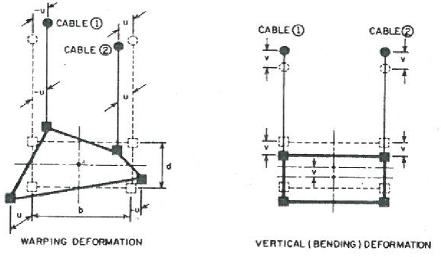
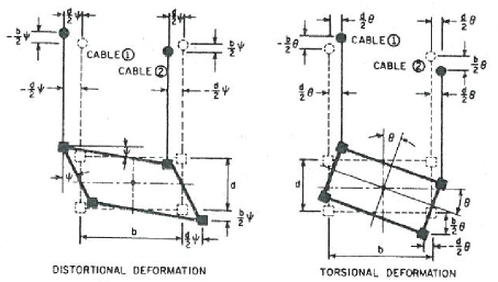
Figure 11: The four different kinds of displacements.

A careful analysis of the energies involved is made, reaching up to fifth derivatives in the equations, see [1, (15)]. Higher order derivatives are then neglected and the following nonlinear system of three PDE’s of fourth order in the three unknown displacements $v$, $\theta$, $\psi$ is obtained, see [1, (28)-(29)-(30)]:

$$\left\{\begin{array}[]{l}\frac{w}{g}\,v_{tt}+EI\,v_{xxxx}-\Big{(}2H_{w}+H_{1}(t)+H_{2}(t)\Big{)}\,v_{xx}+\frac{b}{2}\,\Big{(}H_{1}(t)-H_{2}(t)\Big{)}\,(\theta_{xx}+\psi_{xx})\\ \ \ \ +\frac{w}{2H_{w}}\,\Big{(}H_{1}(t)+H_{2}(t)\Big{)}-\frac{w_{s}\,r^{2}}{g}\,\left(1+\frac{EI}{2G\mu r^{2}}\right)\,v_{xxtt}+\frac{w_{s}^{2}\,r^{2}}{4gG\mu}\,v_{tttt}=0\\ I_{m}\,\theta_{tt}+E\Gamma\,\theta_{xxxx}-GJ\,\theta_{xx}-\frac{H_{w}\,b^{2}}{2}\,(\theta_{xx}+\psi_{xx})-\frac{\gamma\,\Gamma}{g}\,\theta_{xxtt}-\frac{b^{2}}{4}\,\Big{(}H_{1}(t)+H_{2}(t)\Big{)}\,(\theta_{xx}+\psi_{xx})\\ \ \ \ +\frac{b}{2}\,\Big{(}H_{1}(t)-H_{2}(t)\Big{)}\,v_{xx}-\frac{\gamma\,\Lambda}{g}\psi_{xxtt}+\frac{b\,w}{4H_{w}}\,\Big{(}H_{2}(t)-H_{1}(t)\Big{)}+E\Lambda\,\psi_{xxxx}+\frac{w_{c}\,b^{2}}{4g}\,\psi_{tt}=0\\ \frac{w_{c}\,b^{2}}{4g}\,(\psi_{tt}+\theta_{tt})+\frac{EA\,b^{2}d^{2}}{4}\,\psi_{xxxx}-\frac{H_{w}\,b^{2}}{2}\,(\psi_{xx}+\theta_{xx})-\frac{\gamma Ab^{2}d^{2}}{4g}\,\psi_{xxtt}-\frac{\gamma\,\Lambda}{g}\theta_{xxtt}+E\Lambda\,\theta_{xxxx}\\ \ \ \ -\frac{b^{2}}{4}\,\Big{(}H_{1}(t)+H_{2}(t)\Big{)}\,(\theta_{xx}+\psi_{xx})+\frac{b}{2}\,\Big{(}H_{1}(t)-H_{2}(t)\Big{)}\,v_{xx}+\frac{w\,b}{4H_{w}}\,\Big{(}H_{2}(t)-H_{1}(t)\Big{)}=0\ .\end{array}\right.$$

We will not explain here what is the meaning of all the constants involved, it would take several pages… Some of the constants have a clear meaning, for the interpretation of the remaining ones, we refer to [1]. Let us just mention that $H_{1}$ and $H_{2}$ represent the vibrational horizontal components of the cable tension and depend on $v$, $\theta$, $\psi$, and their first derivatives, see [1, (3)]. We wrote these equations in order to convince the reader that the behavior of the bridge is modeled by terribly complicated equations and by no means one should make use of ${\cal LHL}$. After making such huge effort, Abdel-Ghaffar simplifies the problem by neglecting the cross section deformation, the shear deformation and rotatory inertia; he obtains a coupled nonlinear vertical-torsional system of two equations in the two unknowns functions $v$ and $\theta$. These equations are finally linearised, by neglecting $H_{1}$ and $H_{2}$ which are considered small when compared with the initial tension $H_{w}$. Then the coupling effect disappears and equations (6) are recovered, see [1, (34)-(35)]. What a pity, an accurate modeling ended up with a linearisation! But there was no choice… how can one imagine to get any kind of information from the above system?

Summarising, after the previously described pioneering models from [14, 75, 81, 90, 98] there has not been much work among engineers about alternative differential equations; the attention has turned to improving performances through design factors, see e.g. [52], or on how to solve structural problems rather than how to understand them more deeply. In this respect, from [69, p.2] we quote a personal discussion between McKenna and a distinguished civil engineer who said

… having found obvious and effective physical ways of avoiding the problem, engineers will not give too much attention to the mathematical solution of this fascinating puzzle …

Only modeling modern footbridges has attracted some interest from a theoretical point of view. As already mentioned, pedestrian bridges are extremely flexible and display elastic behaviors similar to suspension bridges, although the oscillations are of different kind. In this respect, we would like to mention an interesting discussion with Diana [29]. He explained that when a suspension bridge is attacked by wind its starts oscillating, but soon afterwards the wind itself modifies its behavior according to the bridge oscillation; so, the wind amplifies the oscillations by blowing synchronously. A qualitative description of this phenomenon was already attempted by Rocard [90, p.135]:

… it is physically certain and confirmed by ordinary experience, although the effect is known only qualitatively, that a bridge vibrating with an appreciable amplitude completely imposes its own frequency on the vortices of its wake. It appears as if in some way the bridge itself discharges the vortices into the fluid with a constant phase relationship with its own oscillation… .

This reminds the above described behavior of footbridges where pedestrians fall spontaneously into step with the vibrations: in both cases, external forces synchronise their effect and amplify the oscillations of the bridge. This is one of the reasons why self-excited oscillations appear in suspension and pedestrian bridges.

In [15] a simple 1D model was proposed in order to describe the crowd-flow phenomena occurring when pedestrians walk on a flexible footbridge. The resulting equation [15, (2)] reads

$$\left(m_{s}(x)+m_{p}(x,t)\right)u_{tt}+\delta(x)u_{t}+\gamma(x)u_{xxxx}=g(x,t)$$ (7)

where $x$ is the coordinate along the beam axis, $t$ the time, $u=u(x,t)$ the lateral displacement, $m_{s}(x)$ is the mass per unit length of the beam, $m_{p}(x,t)$ the linear mass of pedestrians, $\delta(x)$ the viscous damping coefficient, $\gamma(x)$ the stiffness per unit length, $g(x,t)$ the pedestrian lateral force per unit length. In view of the superlinear behavior for large displacements observed for the London Millennium Bridge, see Section 2, we wonder if instead of a linear model one should consider a lateral force also depending on the displacement, $g=g(x,t,u)$, being superlinear with respect to $u$.

Problem 2.

Study (7) modified as follows

$$u_{tt}+\delta u_{t}+\gamma u_{xxxx}+f(u)=g(x,t)\qquad(x\in\mathbb{R}\,,\ t>0)$$

where $\delta>0$, $\gamma>0$ and $f(s)=s+\varepsilon s^{3}$ for some $\varepsilon>0$ small. One could first consider the Cauchy problem

$$u(x,0)=u_{0}(x)\ ,\quad u_{t}(x,0)=u_{1}(x)\quad(x\in\mathbb{R})$$

with $g\equiv 0$. Then one could seek traveling waves such as $u(x,t)=w(x-ct)$ which solve the ODE

$$\gamma w^{\prime\prime\prime\prime}(\tau)+c^{2}w^{\prime\prime}(\tau)+\delta cw^{\prime}(\tau)+f(w(\tau))=0\qquad(x-ct=\tau\in\mathbb{R}).$$

Finally, one could also try to find properties of solutions in a bounded interval $x\in(0,L)$. $\Box$

Scanlan-Tomko [96] introduce a model in which the torsional angle $\theta$ of the roadway section satisfies the equation

$$I\,[\theta^{\prime\prime}(t)+2\zeta_{\theta}\omega_{\theta}\theta^{\prime}(t)+\omega_{\theta}^{2}\theta(t)]=A\theta^{\prime}(t)+B\theta(t)\ ,$$ (8)

where $I$, $\zeta_{\theta}$, $\omega_{\theta}$ are, respectively, associated inertia, damping ratio, and natural frequency. The r.h.s. of (8) represents the aerodynamic force and was postulated to depend linearly on both $\theta^{\prime}$ and $\theta$ with the positive constants $A$ and $B$ depending on several parameters of the bridge. Since (8) may be seen as a two-variables first order linear system, it fails to fulfill both the requirements of (GP). Hence, (8) is not suitable to describe the disordered behavior of a bridge. And indeed, elementary calculus shows that if $A$ is sufficiently large, then solutions to (8) are positive exponentials times trigonometric functions which do not exhibit a sudden appearance of self-excited oscillations, they merely blow up in infinite time. In order to have a more reliable description of the bridge, in Section 4 we consider the fourth order nonlinear ODE $w^{\prime\prime\prime\prime}+kw^{\prime\prime}+f(w)=0$ ($k\in\mathbb{R}$). We will see that solutions to this equation blow up in finite time with self-excited oscillations appearing suddenly, without any intermediate stage.

That linearisation yields wrong models is also the opinion of McKenna [69, p.4] who comments (8) by writing

This is the point at which the discussion of torsional oscillation starts in the engineering literature.

He claims that the problem is in fact nonlinear and that (8) is obtained after an incorrect linearisation. McKenna concludes by noticing that

Even in recent engineering literature … this same mistake is reproduced.

The mistake claimed by McKenna is that the equations are often linearised by taking $\sin\theta=\theta$ and $\cos\theta=1$ also for large amplitude torsional oscillations $\theta$. The corresponding equation then becomes linear and the main torsional phenomenon disappears. Avoiding this rude approximation, but considering the cables and hangers as linear springs obeying ${\cal LHL}$, McKenna reaches an uncoupled second order system for the functions representing the vertical displacement $y$ of the barycenter $B$ of the cross section of the roadway and the deflection from horizontal $\theta$, see Figure 12. Here, $2\ell$ denotes the width of the roadway whereas $C_{1}$ and $C_{2}$ denote the two lateral hangers which have opposite extension behaviors.

Figure 12: Vertical displacement and deflection of the cross section of the roadway.

McKenna-Tuama [72] suggest a slightly different model. They write:

… there should be some torsional forcing. Otherwise, there would be no input of energy to overcome the natural damping of the system … we expect the bridge to behave like a stiff spring, with a restoring force that becomes somewhat superlinear.

We completely agree with this, see the conclusions in Section 6. McKenna-Tuama end up with the following coupled second order system

$$\frac{m\ell^{2}}{3}\,\theta^{\prime\prime}=\ell\cos\theta\,\Big{(}f(y-\ell\sin\theta)-f(y+\ell\sin\theta)\Big{)}\ ,\quad m\,y^{\prime\prime}=-\Big{(}f(y-\ell\sin\theta)+f(y+\ell\sin\theta)\Big{)}\ ,$$ (9)

see again Figure 12. The delicate point is the choice of the superlinearity $f$ which [72] take first as $f(s)=(s+1)^{+}-1$ and then as $f(s)=e^{s}-1$ in order to maintain the asymptotically linear behavior as $s\to 0$. Using (9), [69, 72] were able to numerically replicate the phenomenon observed at the Tacoma Bridge, namely the sudden transition from vertical oscillations to torsional oscillations. They found that if the vertical motion was sufficiently large to induce brief slackening of the hangers, then numerical results highlighted a rapid transition to a torsional motion. Nevertheless, the physicists Green-Unruh [50] believe that the hangers were not slack during the Tacoma Bridge oscillation. If this were true, then the piecewise linear forcing term $f$ becomes totally linear. Moreover, by commenting the results in [69, 72], McKenna-Moore [71, p.460] write that

…the range of parameters over which the transition from vertical to torsional motion was observed was physically unreasonable … the restoring force due to the cables was oversimplified … it was necessary to impose small torsional forcing.

Summarising, (9) seems to be the first model able to reproduce the behavior of the Tacoma Bridge but it appears to need some improvements. First, one should avoid the possibility of a linear behavior of the hangers, the nonlinearity should appear before possible slackening of the hangers. Second, the restoring force and the parameters involved should be chosen carefully.

Problem 3.

Try a doubly superlinear term $f$ in (9). For instance, take $f(s)=s+\varepsilon s^{3}$ with $\varepsilon>0$ small, so that (9) becomes

$$\frac{m\ell^{2}}{3}\,\theta^{\prime\prime}+2\ell^{2}\cos\theta\sin\theta\,\Big{(}1+3\varepsilon y^{2}+\varepsilon\ell^{2}\sin^{2}\theta\Big{)}=0\ ,\quad m\,y^{\prime\prime}+2\Big{(}1+3\varepsilon\ell^{2}\sin^{2}\theta\Big{)}y+2\varepsilon y^{3}=0\ .$$ (10)

It appears challenging to determine some features of the solution $(y,\theta)$ to (10) and also to perform numerical experiments to see what kind of oscillations are displayed by the solutions. $\Box$

System (9) is a $2\times 2$ system which should be considered as a nonlinear fourth order model; therefore, it fulfills the necessary conditions of the general principle (GP). Another fourth order differential equation was suggested in [62, 73, 74] as a one-dimensional model for a suspension bridge, namely a beam of length $L$ suspended by hangers. When the hangers are stretched there is a restoring force which is proportional to the amount of stretching, according to ${\cal LHL}$. But when the beam moves in the opposite direction, there is no restoring force exerted on it. Under suitable boundary conditions, if $u(x,t)$ denotes the vertical displacement of the beam in the downward direction at position $x$ and time $t$, the following nonlinear beam equation is derived

$$u_{tt}+u_{xxxx}+\gamma u^{+}=W(x,t)\,,\qquad x\in(0,L)\,,\quad t>0\,,$$ (11)

where $u^{+}=\max\{u,0\}$, $\gamma u^{+}$ represents the force due to the cables and hangers which are considered as a linear spring with a one-sided restoring force, and $W$ represents the forcing term acting on the bridge, including its own weight per unit length, the wind, the traffic loads, or other external sources. After some normalisation, by seeking traveling waves $u(x,t)=1+w(x-ct)$ to (11) and putting $k=c^{2}>0$, McKenna-Walter [74] reach the following ODE

$$w^{\prime\prime\prime\prime}(\tau)+kw^{\prime\prime}(\tau)+f(w(\tau))=0\qquad(x-ct=\tau\in\mathbb{R})$$ (12)

where $k\in(0,2)$ and $f(s)=(s+1)^{+}-1$. Subsequently, in order to maintain the same behavior but with a smooth nonlinearity, Chen-McKenna [21] suggest to consider (12) with $f(s)=e^{s}-1$. For later discussion, we notice that both these nonlinearities satisfy

$$f\in{\rm Lip}_{{\rm loc}}(\mathbb{R})\,,\quad f(s)\,s>0\quad\forall s\in\mathbb{R}\setminus\{0\}.$$ (13)

Hence, when $W\equiv 0$, (11) is just a special case of the more general semilinear fourth order wave equation

$$u_{tt}+u_{xxxx}+f(u)=0\,,\qquad x\in(0,L)\,,\quad t>0\,,$$ (14)

where the natural assumptions on $f$ are (13) plus further conditions, according to the model considered. Traveling waves to (14) solve (12) with $k=c^{2}$ being the squared velocity of the wave. Recently, for $f(s)=(s+1)^{+}-1$ and its variants, Benci-Fortunato [10] proved the existence of special solutions to (12) deduced by solitons of the beam equation (14).

Problem 4.

It could be interesting to insert into the wave-type equation (14) the term corresponding to the beam elongation, that is,

$$\int_{0}^{L}\Big{(}\sqrt{1+u_{x}(x,t)^{2}}-1\Big{)}\,dx.$$

This would lead to a quasilinear equation such as

$$u_{tt}+u_{xxxx}-\left(\frac{u_{x}}{\sqrt{1+u_{x}^{2}}}\right)_{x}+f(u)=0$$

with $f$ satisfying (13). What can be said about this equation? Does it admit oscillating solutions in a suitable sense? One should first consider the case of an unbounded beam ($x\in\mathbb{R}$) and then the case of a bounded beam ($x\in(0,L)$) complemented with some boundary conditions. $\Box$

Motivated by the fact that it appears unnatural to ignore the motion of the main sustaining cable, a slightly more sophisticated and complicated string-beam model was suggested by Lazer-McKenna [63]. They treat the cable as a vibrating string, coupled with the vibrating beam of the roadway by piecewise linear springs that have a given spring constant $k$ if expanded, but no restoring force if compressed. The sustaining cable is subject to some forcing term such as the wind or the motions in the towers. This leads to the system

$$\left\{\begin{array}[]{ll}v_{tt}-c_{1}v_{xx}+\delta_{1}v_{t}-k_{1}(u-v)^{+}=f(x,t)\,,\qquad x\in(0,L)\,,\quad t>0\,,\\ u_{tt}+c_{2}u_{xxxx}+\delta_{2}u_{t}+k_{2}(u-v)^{+}=W_{0}\,,\qquad x\in(0,L)\,,\quad t>0\,,\end{array}\right.$$

where $v$ is the displacement from equilibrium of the cable and $u$ is the displacement of the beam, both measured in the downwards direction. The constants $c_{1}$ and $c_{2}$ represent the relative strengths of the cables and roadway respectively, whereas $k_{1}$ and $k_{2}$ are the spring constants and satisfy $k_{2}\ll k_{1}$. The two damping terms can possibly be set to $0$, while $f$ and $W_{0}$ are the forcing terms. We also refer to [2] for a study of the same problem in a rigorous functional analytic setting.

Since the Tacoma Bridge collapse was mainly due to a wide torsional motion of the bridge, see [116], the bridge cannot be considered as a one dimensional beam. In this respect, Rocard [90, p.148] states

Conventional suspension bridges are fundamentally unstable in the wind because the coupling effect introduced between bending and torsion by the aerodynamic forces of the lift.

Hence, if some model wishes to display instability of bridges, it should necessarily take into account more degrees of freedom than just a beam. In fact, to be exhaustive one should consider vertical oscillations $y$ of the roadway, its torsional angle $\theta$, and coupling with the two sustaining cables $u$ and $v$. This model was suggested by Matas-Očenášek [68] who consider the hangers as linear springs and obtain a system of four equations; three of them are second order wave-type equations, the last one is again a fourth order equation such as

$$m\,y_{tt}+k\,y_{xxxx}+\delta\,y_{t}+E_{1}(y-u-\ell\sin\theta)+E_{2}(y-v+\ell\sin\theta)=W(x)+f(x,t)\ ;$$

we refer to $(SB_{4})$ in [30] for an interpretation of the parameters involved.

In our opinion, any model which describes the bridge as a one dimensional beam is too simplistic, unless the model takes somehow into account the possible appearance of a torsional motion. In [46] it was suggested to maintain the one dimensional model provided one also allows displacements below the equilibrium position and these displacements replace the deflection from horizontal of the roadway of the bridge; in other words,

$$\begin{array}[]{c}\mbox{the unknown function $w$ represents the upwards vertical displacement when $w>0$}\\ \mbox{and the deflection from horizontal, computed in a suitable unity measure, when $w<0$.}\end{array}$$ (15)

In this setting, instead of (11) one should consider the more general semilinear fourth order wave equation (14) with $f$ satisfying (13) plus further conditions which make $f(s)$ superlinear and unbounded when both $s\to\pm\infty$; hence, ${\cal LHL}$ is dropped by allowing $f$ to be as close as one may wish to a linear function but eventually superlinear for large displacements. The superlinearity assumption is justified both by the observations in Section 2 and by the fact that more the position of the bridge is far from the horizontal equilibrium position, more the action of the wind becomes relevant because the wind hits transversally the roadway of the bridge. If ever the bridge would reach the limit vertical position, in case the roadway is torsionally rotated of a right angle, the wind would hit it orthogonally, that is, with full power.

In this section we listed a number of attempts to model bridges mechanics by means of differential equations. The sources for this list are very heterogeneous. However, except for some possible small damping term, none of them contains odd derivatives. Moreover, none of them is acknowledged by the scientific community to perfectly describe the complex behavior of bridges. Some of them fail to satisfy the requirements of (GP) and, in our opinion, must be accordingly modified. Some others seem to better describe the oscillating behavior of bridges but still need some improvements.

4 Blow up oscillating solutions to some fourth order differential equations

If the trivial solution to some dynamical system is unstable one may hope to magnify self-excitement phenomena through finite time blow up. In this section we survey and discuss several results about solutions to (12) which blow up in finite time. Let us rewrite the equation with a different time variable, namely

$$w^{\prime\prime\prime\prime}(t)+kw^{\prime\prime}(t)+f(w(t))=0\qquad(t\in\mathbb{R})\ .$$ (16)

We first recall the following results proved in [12]:

Theorem 5.

Let $k\in\mathbb{R}$ and assume that $f$ satisfies (13).

$(i)$ If a local solution $w$ to (16) blows up at some finite $R\in\mathbb{R}$, then

$$\liminf_{t\to R}w(t)=-\infty\qquad\mbox{and}\qquad\limsup_{t\to R}w(t)=+\infty\,.$$ (17)

$(ii)$ If $f$ also satisfies

$$\limsup_{s\to+\infty}\frac{f(s)}{s}<+\infty\qquad\mbox{or}\qquad\limsup_{s\to-\infty}\frac{f(s)}{s}<+\infty,$$ (18)

then any local solution to (16) exists for all $t\in\mathbb{R}$.

If both the conditions in (18) are satisfied then global existence follows from classical theory of ODE’s; but (18) merely requires that $f$ is “one-sided at most linear” so that statement $(ii)$ is far from being trivial and, as shown in [46], it does not hold for equations of order at most 3. On the other hand, Theorem 5 $(i)$ states that, under the sole assumption (13), the only way that finite time blow up can occur is with “wide and thinning oscillations” of the solution $w$; again, in [46] it was shown that this kind of blow up is a phenomenon typical of at least fourth order problems such as (16) since it does not occur in related lower order equations. Note that assumption (18) includes, in particular, the cases where $f$ is either concave or convex.

Theorem 5 does not guarantee that the blow up described by (17) indeed occurs. For this reason, we assume further that

$$f\in{\rm Lip}_{{\rm loc}}(\mathbb{R})\cap C^{2}(\mathbb{R}\setminus\{0\})\ ,\quad f^{\prime}(s)\geq 0\quad\forall s\in\mathbb{R}\ ,\quad\liminf_{s\to\pm\infty}|f^{\prime\prime}(s)|>0$$ (19)

and the growth conditions

$$\exists p>q\geq 1,\ \alpha\geq 0,\ 0<\rho\leq\beta,\quad\mbox{s.t.}\quad\rho|s|^{p+1}\leq f(s)s\leq\alpha|s|^{q+1}+\beta|s|^{p+1}\quad\forall s\in\mathbb{R}\ .$$ (20)

Notice that (19)-(20) strengthen (13). In [48] the following sufficient conditions for the finite time blow up of local solutions to (16) has been proved.

Theorem 6.

Let $k\leq 0$, $p>q\geq 1$, $\alpha\geq 0$, and assume that $f$ satisfies (19) and (20). Assume that $w=w(t)$ is a local solution to (16) in a neighborhood of $t=0$ which satisfies

$$w^{\prime}(0)w^{\prime\prime}(0)-w(0)w^{\prime\prime\prime}(0)-kw(0)w^{\prime}(0)>0\,.$$ (21)

Then, $w$ blows up in finite time for $t>0$, that is, there exists $R\in(0,+\infty)$ such that (17) holds.

Since self-excited oscillations such as (17) should be expected in any equation attempting to model suspension bridges, linear models should be avoided. Unfortunately, even if the solutions to (16) display these oscillations, they cannot be prevented since they arise suddenly after a long time of apparent calm. In Figure 13, we display the plot of a solution to (16).

Figure 13: Solution to (16) for $k=3$, $[w(0),w^{\prime}(0),w^{\prime\prime}(0),w^{\prime\prime\prime}(0)]=[1,0,0,0]$, $f(s)=s+s^{3}$. The three intervals are $t\in[0,7]$, $t\in[7,8]$, $t\in[8,8.16]$

It can be observed that the solution has oscillations with increasing amplitude and rapidly decreasing “nonlinear frequency”; numerically, the blow up seems to occur at $t=8.164$. Even more impressive appears the plot in Figure 14.

Figure 14: Solution to (16) for $k=3.6$, $[w(0),w^{\prime}(0),w^{\prime\prime}(0),w^{\prime\prime\prime}(0)]=[0.9,0,0,0]$, $f(s)=s+s^{3}$. The three intervals are $t\in[0,80]$, $t\in[80,95]$, $t\in[95,96.55]$

Here the solution has “almost regular” oscillations between $-1$ and $+1$ for $t\in[0,80]$. Then the amplitude of oscillations nearly doubles in the interval $[80,93]$ and, suddenly, it violently amplifies after $t=96.5$ until the blow up which seems to occur only slightly later at $t=96.59$. We also refer to [46, 47, 48] for further plots.

We refer to [46, 48] for numerical results and plots of solutions to (16) with nonlinearities $f=f(s)$ having different growths as $s\to\pm\infty$. In such case, the solution still blows up according to (17) but, although its “limsup” and “liminf” are respectively $+\infty$ and $-\infty$, the divergence occurs at different rates. We represent this qualitative behavior in Figure 15.

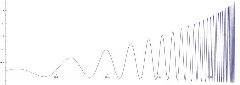
Figure 15: Qualitative blow up for solutions to (16) when $f(s)$ is superlinear at different rates as $s\to\pm\infty$.

Traveling waves to (14) which propagate at some velocity $c>0$, depending on the elasticity of the material of the beam, solve (16) with $k=c^{2}>0$. Further numerical results obtained in [46, 48] suggest that a statement similar to Theorem 6 also holds for $k>0$ and, as expected, that the blow up time $R$ is decreasing with respect to the initial height $w(0)$ and increasing with respect to $k$. Since $k=c^{2}$ and $c$ represents the velocity of the traveling wave, this means that the time of blow up is an increasing function of $k$. In turn, since the velocity of the traveling wave depends on the elasticity of the material used to construct the bridge (larger $c$ means less elastic), this tells us that more the bridge is stiff more it will survive to exterior forces such as the wind and/or traffic loads.

Problem 7.

Prove Theorem 6 when $k>0$. This would allow to show that traveling waves to (14) blow up in finite time. Numerical results in [46, 48] suggest that a result similar to Theorem 6 also holds for $k>0$. $\Box$

Problem 8.

Prove that the blow up time of solutions to (16) depends increasingly with respect to $k\in\mathbb{R}$. The interest of an analytical proof of this fact relies on the important role played by $k$ within the model. $\Box$

Problem 9.

The blow up time $R$ of solutions to (16) is the expectation of life of the oscillating bridge. Provide an estimate of $R$ in terms of $f$ and of the initial data. $\Box$

Problem 10.

Condition (20) is a superlinearity assumption which requires that $f$ is bounded both from above and below by the same power $p>1$. Prove Theorem 6 for more general kinds of superlinear functions $f$. $\Box$

Problem 11.

Can assumption (21) be relaxed? Of course, it cannot be completely removed since the trivial solution $w(t)\equiv 0$ is globally defined, that is, $R=+\infty$. Numerical experiments in [46, 48] could not detect any nontrivial global solution to (16). $\Box$

Problem 12.

Study (16) with a damping term: $w^{\prime\prime\prime\prime}(t)+kw^{\prime\prime}(t)+\delta w^{\prime}(t)+f(w(t))=0$ for some $\delta>0$. Study the competition between the damping term $\delta w^{\prime}$ and the nonlinear self-exciting term $f(w)$. $\Box$

Note that Theorems 5 and 6 ensure that there exists an increasing sequence $\{z_{j}\}_{j\in\mathbb{N}}$ such that:

$(i)$ $z_{j}\nearrow R$ as $j\to\infty$;

$(ii)$ $w(z_{j})=0$ and $w$ has constant sign in $(z_{j},z_{j+1})$ for all $j\in\mathbb{N}$.

It is also interesting to compare the rate of blow up of the displacement and of the acceleration on these intervals. By slightly modifying the proof of [48, Theorem 3] one can obtain the following result which holds for any $k\in\mathbb{R}$.

Theorem 13.

Let $k\in\mathbb{R}$, $p>q\geq 1$, $\alpha\geq 0$, and assume that $f$ satisfies (19) and (20). Assume that $w=w(t)$ is a local solution to

$$w^{\prime\prime\prime\prime}(t)+kw^{\prime\prime}(t)+f(w(t))=0\qquad(t\in\mathbb{R})$$

which blows up in finite time as $t\nearrow R<+\infty$. Denote by $\{z_{j}\}$ the increasing sequence of zeros of $w$ such that $z_{j}\nearrow R$ as $j\to+\infty$. Then

$$\int_{z_{j}}^{z_{j+1}}w(t)^{2}\,dt\ \ll\ \int_{z_{j}}^{z_{j+1}}w^{\prime\prime}(t)^{2}\,dt\ ,\qquad\int_{z_{j}}^{z_{j+1}}w^{\prime}(t)^{2}\,dt\ \ll\ \int_{z_{j}}^{z_{j+1}}w^{\prime\prime}(t)^{2}\,dt$$ (22)

as $j\to\infty$. Here, $g(j)\ll\psi(j)$ means that $g(j)/\psi(j)\to 0$ as $j\to\infty$.

The estimate (22), clearly due to the superlinear term, has a simple interpretation in terms of comparison between blowing up energies, see Section 5.1.

Remark 14.

Equation (16) also arises in several different contexts, see the book by Peletier-Troy [84] where one can find some other physical models, a survey of existing results, and further references. Moreover, besides (14), (16) may also be fruitfully used to study some other partial differential equations. For instance, one can consider nonlinear elliptic equations such as

$$\Delta^{2}u+e^{u}=\frac{1}{|x|^{4}}\qquad\mbox{in }\mathbb{R}^{4}\setminus\{0\}\ ,$$

$$\Delta^{2}u+|u|^{8/(n-4)}u=0\mbox{ in }\mathbb{R}^{n}\ (n\geq 5),\qquad\Delta\Big{(}|x|^{2}\Delta u\Big{)}+|x|^{2}|u|^{8/(n-2)}u=0\mbox{ in }\mathbb{R}^{n}\ (n\geq 3);$$ (23)

it is known (see, e.g. [45]) that the Green function for some fourth order elliptic problems displays oscillations, differently from second order problems. Furthermore, one can also consider the semilinear parabolic equation

$$u_{t}+\Delta^{2}u=|u|^{p-1}u\mbox{ in }\mathbb{R}_{+}^{n+1}\ ,\qquad u(x,0)=u_{0}(x)\mbox{ in }\mathbb{R}^{n}$$

where $p>1+4/n$ and $u_{0}$ satisfies suitable assumptions. It is shown in [40, 44] that the linear biharmonic heat operator has an “eventual local positivity” property: for positive initial data $u_{0}$ the solution to the linear problem with no source is eventually positive on compact subsets of $\mathbb{R}^{n}$ but negativity can appear at any time far away from the origin. This phenomenon is due to the sign changing properties, with infinite oscillations, of the biharmonic heat kernels. We also refer to [12, 48] for some results about the above equations and for the explanation of how they can be reduced to (16) and, hence, how they display self-excited oscillations. $\Box$

Problem 15.

For any $q>0$ and parameters $a,b,k\in\mathbb{R}$, $c\geq 0$, study the equation

$$w^{\prime\prime\prime\prime}(t)+aw^{\prime\prime\prime}(t)+kw^{\prime\prime}(t)+bw^{\prime}(t)+cw(t)+|w(t)|^{q}w(t)=0\qquad(t\in\mathbb{R})\ .$$ (24)

Any reader who is familiar with the second order Sobolev space $H^{2}$ recognises the critical exponent in the first equation in (23). In view of Liouville-type results in [27] when $q\leq 8/(n-4)$, it would be interesting to study the equation $\Delta^{2}u+|u|^{q}u=0$ with the same technique. The radial form of this equation may be written as (16) only when $q=8/(n-4)$ since for other values of $q$ the transformation in [43] gives rise to the appearance of first and third order derivatives as in (24): this motivates (24). The values of the parameters corresponding to the equation $\Delta^{2}u+|u|^{q}u=0$ can be found in [43]. $\Box$

Our target is now to reproduce the self-excited oscillations found in Theorem 6 in a suitable second order system. Replace $\sin\theta\cong\theta$ and $\cos\theta\cong 1$, and put $x=\ell\theta$. After these transformations, the McKenna system (9) reads

$$\left\{\begin{array}[]{ll}x^{\prime\prime}+\omega^{2}f(y+x)-\omega^{2}f(y-x)=0\\ y^{\prime\prime}+f(y+x)+f(y-x)=0\ .\end{array}\right.$$ (25)

We further modify (25); for suitable values of the parameters $\beta$ and $\delta$, we consider the system

$$\left\{\begin{array}[]{ll}x^{\prime\prime}-f(y-x)+\beta(y+x)=0\\ y^{\prime\prime}-f(y-x)+\delta(y+x)=0\end{array}\right.$$ (26)

which differs from (25) in two respects: the minus sign in front of $f(y-x)$ in the second equation and the other restoring force $f(y+x)$ being replaced by a linear term. To (26) we associate the initial value problem

$$x(0)=x_{0}\,,\ x^{\prime}(0)=x_{1}\,,\ y(0)=y_{0}\,,\ y^{\prime}(0)=y_{1}\ .$$ (27)

The following statement holds.

Theorem 16.

Assume that $\beta<\delta\leq-\beta$ (so that $\beta<0$). Assume also that $f(s)=\sigma s+cs^{2}+ds^{3}$ with $d>0$ and $c^{2}\leq 2d\sigma$. Let $(x_{0},y_{0},x_{1},y_{1})\in\mathbb{R}^{4}$ satisfy

$$(3\beta-\delta)x_{0}y_{1}+(3\delta-\beta)x_{1}y_{0}>(\beta+\delta)(x_{0}x_{1}+y_{0}y_{1})\ .$$ (28)

If $(x,y)$ is a local solution to (26)-(27) in a neighborhood of $t=0$, then $(x,y)$ blows up in finite time for $t>0$ with self-excited oscillations, that is, there exists $R\in(0,+\infty)$ such that

$$\liminf_{t\to R}x(t)=\liminf_{t\to R}y(t)=-\infty\qquad\mbox{and}\qquad\limsup_{t\to R}x(t)=\limsup_{t\to R}y(t)=+\infty\,.$$

Proof. After performing the change of variables (53), system (26) becomes

$$w^{\prime\prime}+(\delta-\beta)z=0\ ,\qquad z^{\prime\prime}-2f(w)+(\beta+\delta)z=0$$

which may be rewritten as a single fourth order equation

$$w^{\prime\prime\prime\prime}(t)+(\beta+\delta)w^{\prime\prime}(t)+2(\delta-\beta)f(w(t))=0\ .$$ (29)

Assumption (28) reads

$$w^{\prime}(0)w^{\prime\prime}(0)-w(0)w^{\prime\prime\prime}(0)-(\beta+\delta)w(0)w^{\prime}(0)>0\,.$$

Furthermore, in view of the above assumptions, $f$ satisfies (19)-(20) with $\rho=d/2$, $p=3$, $\alpha=2\sigma$, $q=1$, $\beta=3d$. Whence, Theorem 13 states that $w$ blows up in finite time for $t>0$ and that there exists $R\in(0,+\infty)$ such that

$$\liminf_{t\to R}w(t)=-\infty\qquad\mbox{and}\qquad\limsup_{t\to R}w(t)=+\infty\,.$$ (30)

Next, we remark that (29) admits a first integral, namely

$$E(t) := \frac{\beta+\delta}{2}\,w^{\prime}(t)^{2}+w^{\prime}(t)w^{\prime\prime\prime}(t)+2(\delta-\beta)F(w(t))-\frac{1}{2}\,w^{\prime\prime}(t)^{2}$$

$$= \frac{\beta+\delta}{2}\,w^{\prime}(t)^{2}+(\beta-\delta)w^{\prime}(t)z^{\prime}(t)+2(\delta-\beta)F(w(t))-\frac{(\beta-\delta)^{2}}{2}\,z(t)^{2}\equiv\overline{E}\ ,$$ (31)

for some constant $\overline{E}$. By (30) there exists an increasing sequence $m_{j}\to R$ of local maxima of $w$ such that

$$z(m_{j})=\frac{w^{\prime\prime}(m_{j})}{\beta-\delta}\geq 0\ ,\quad w^{\prime}(m_{j})=0\ ,\quad w(m_{j})\to+\infty\mbox{ as }j\to\infty\ .$$

By plugging $m_{j}$ into the first integral (31) we obtain

$$\overline{E}=E(m_{j})=2(\delta-\beta)F(w(m_{j}))-\frac{(\beta-\delta)^{2}}{2}\,z(m_{j})^{2}$$

which proves that $z(m_{j})\to+\infty$ as $j\to+\infty$. We may proceed similarly in order to show that $z(\mu_{j})\to-\infty$ on a sequence $\{\mu_{j}\}$ of local minima of $w$. Therefore, we have

$$\liminf_{t\to R}z(t)=-\infty\qquad\mbox{and}\qquad\limsup_{t\to R}z(t)=+\infty\,.$$

Assume for contradiction that there exists $K\in\mathbb{R}$ such that $x(t)\leq K$ for all $t<R$. Then, recalling (53), on the above sequence $\{m_{j}\}$ of local maxima for $w$, we would have $y(m_{j})-K\geq y(m_{j})-x(m_{j})=w(m_{j})\to+\infty$ which is incompatible with (31) since

$$2(\delta-\beta)F(y(m_{j})-x(m_{j}))-\frac{(\beta-\delta)^{2}}{2}\,(y(m_{j})+x(m_{j}))^{2}\equiv\overline{E}$$

and $F$ has growth of order 4 with respect to its divergent argument. Similarly, by arguing on the sequence $\{\mu_{j}\}$, we rule out the possibility that there exists $K\in\mathbb{R}$ such that $x(t)\geq K$ for ll $t<R$. Finally, by changing the role of $x$ and $y$ we find that also $y(t)$ is unbounded both from above and below as $t\to R$. This completes the proof. $\Box$

Remark 17.

Numerical results in [48] suggest that the assumption $\delta\leq-\beta$ is not necessary to obtain (30). So, most probably, Theorem 16 and the results of this section hold true also without this assumption. $\Box$

A special case of function $f$ satisfying the assumptions of Theorem 16 is $f_{\varepsilon}(s)=s+\varepsilon s^{3}$ for any $\varepsilon>0$. We wish to study the situation when the problem tends to become linear, that is, when $\varepsilon\to 0$. Plugging such $f_{\varepsilon}$ into (26) gives the system

$$\left\{\begin{array}[]{ll}x^{\prime\prime}+(\beta+1)x+(\beta-1)y+\varepsilon(x-y)^{3}=0\\ y^{\prime\prime}+(\delta+1)x+(\delta-1)y+\varepsilon(x-y)^{3}=0\end{array}\right.$$ (32)

so that the limit linear problem obtained for $\varepsilon=0$ reads

$$\left\{\begin{array}[]{ll}x^{\prime\prime}+(\beta+1)x+(\beta-1)y=0\\ y^{\prime\prime}+(\delta+1)x+(\delta-1)y=0\ .\end{array}\right.$$ (33)

The theory of linear systems tells us that the shape of the solutions to (33) depends on the signs of the parameters

$$A=\beta+\delta\ ,\quad B=2(\delta-\beta)\ ,\quad\Delta=(\beta+\delta)^{2}+8(\beta-\delta)\ .$$

Under the same assumptions of Theorem 16, for (33) we have $A\leq 0$ and $B>0$ but the sign of $\Delta$ is not known a priori and three different cases may occur.

$\bullet$ If $\Delta<0$ (a case including also $A=0$), then we have exponentials times trigonometric functions so either we have self-excited oscillations which increase amplitude as $t\to\infty$ or we have damped oscillations which tend to vanish as $t\to\infty$. Consider the case $\delta=-\beta=1$ and $(x_{0},y_{0},x_{1},y_{1})=(1,0,1,-1)$, then (28) is fulfilled and Theorem 16 yields

Corollary 18.

For any $\varepsilon>0$ there exists $R_{\varepsilon}>0$ such that the solution $(x^{\varepsilon},y^{\varepsilon})$ to the Cauchy problem

$$\left\{\begin{array}[]{ll}x^{\prime\prime}-2y+\varepsilon(x-y)^{3}=0\\ y^{\prime\prime}+2x+\varepsilon(x-y)^{3}=0\\ x(0)=1,\ y(0)=0,\ x^{\prime}(0)=1,\ y^{\prime}(0)=-1\end{array}\right.$$ (34)

blows up as $t\to R_{\varepsilon}$ and satisfies

$$\liminf_{t\to R_{\varepsilon}}x^{\varepsilon}(t)=\liminf_{t\to R_{\varepsilon}}y^{\varepsilon}(t)=-\infty\qquad\mbox{and}\qquad\limsup_{t\to R_{\varepsilon}}x^{\varepsilon}(t)=\limsup_{t\to R_{\varepsilon}}y^{\varepsilon}(t)=+\infty\,.$$

A natural conjecture, supported by numerical experiments, is that $R_{\varepsilon}\to\infty$ as $\varepsilon\to 0$. For several $\varepsilon>0$, we plotted the solution to (34) and the pictures all looked like Figure 16.

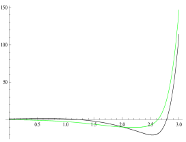
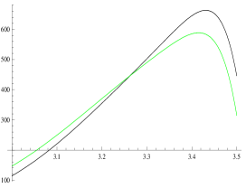
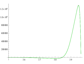
Figure 16: The solution $x^{\varepsilon}$ (black) and $y^{\varepsilon}$ (green) to (34) for $\varepsilon=0.1$.

When $\varepsilon=0.1$ the blow up seems to occur at $R_{\varepsilon}=4.041$. Notice that $x^{\varepsilon}$ and $y^{\varepsilon}$ “tend to become the same”, in the third picture they are indistinguishable. After some time, when wide oscillations amplifies, $x^{\varepsilon}$ and $y^{\varepsilon}$ move almost synchronously. When $\varepsilon=0$, the solution to (34) is explicitly given by $x^{0}(t)=e^{t}\cos(t)$ and $y^{0}(t)=-e^{t}\sin(t)$, thereby displaying oscillations blowing up in infinite time similar to those visible in (8).

If we replace the Cauchy problem in (34) with

$$x(0)=1,\ y(0)=0,\ x^{\prime}(0)=-1,\ y^{\prime}(0)=1$$

then (28) is not fulfilled. However, for any $\varepsilon>0$ that we tested, the corresponding numerical solutions looked like in Figure 16. In this case, the limit problem with $\varepsilon=0$ admits as solutions $x^{0}(t)=e^{-t}\cos(t)$ and $y^{0}(t)=e^{-t}\sin(t)$ which do exhibit oscillations but, now, strongly damped.

Let us also consider the two remaining limit systems which, however, do not display oscillations.

$\bullet$ If $\Delta=0$, since $A\leq 0$, there are no trigonometric functions in the limit case (33).

$\bullet$ If $\Delta>0$, then necessarily $A<0$ since $B>0$, and hence only exponential functions are involved: the solution to (33) may blow up in infinite time or vanish at infinity.

The above results explain why we believe that (8) is not suitable to display self-excited oscillations as the ones which appeared for the TNB. Since it has only two degrees of freedom, it fails to consider both vertical and torsional oscillations which, on the contrary, are visible in the McKenna-type system (26). We have seen in Theorem 16 that destructive self-excited oscillations may blow up in finite time, something very similar to what may be observed in [116]. Hence, (26) shows more realistic self-excited oscillations than (8).

Although the blow up occurs at $t=4.04$, the solution plotted in Figure 16 is relatively small until $t=3.98$. This, together with the behavior displayed in Figures 13 and 14, allows us to conclude that

in nonlinear systems, self-excited oscillations appear suddenly, without any intermediate stage.

The material presented in this section also enables us to conclude that

the linear case cannot be seen as a limit situation of the nonlinear case

since the behavior of the solution to (33) depends on $\beta$, $\delta$, and on the initial conditions, while nothing can be deduced from the sequence of solutions $(x^{\varepsilon},y^{\varepsilon})$ to problem (32) as $\varepsilon\to 0$ because these solutions all behave similarly independently of $\beta$ and $\delta$. Furthermore, the solutions to the limit problem (33) may or may not exhibit oscillations and if they do, these oscillations may be both of increasing amplitude or of vanishing amplitude as $t\to+\infty$. All this shows that linearisation may give misleading and unpredictable answers.

In this section we have seen that the blow up of solutions to (16) and to (26) occurs with wide oscillations after a long time of apparent calm. Hence, the solution does not display any visible behavior which may warn some imminent danger. The reason is that second derivatives of the solution to (16) blow up at a higher rate, see Theorem 13, and second derivatives are not visible by simply looking at the graph. Wide oscillations after a long time of apparent calm suggest that some hidden energy is present in the system. Finally, we have seen that self-excited oscillating blow up also appears for a wide class of superlinear fourth order differential equations, including PDE’s.

5 Affording an explanation in terms of energies

5.1 Energies involved

The most important tools to describe any structure are the energies which appear. A precise description of all the energies involved would lead to perfect models and would give all the information to make correct projects. Unfortunately, bridges, as well as many other structures, do not allow simple characterisations of all the energies present in the structure and, maybe, not all possible existing energies have been detected up to nowadays. Hence, it appears impossible to make a precise list of all the energies involved in the complex behavior of a bridge.

The kinetic energy is the simplest energy to be described. If $v(x,t)$ denotes the vertical displacement at $x\in\Omega$ and at $t>0$, then the total kinetic energy at time $t$ is given by

$$\frac{m}{2}\int_{\Omega}v_{t}(x,t)^{2}\,dx$$

where $m$ is the mass and $\Omega$ can be either a segment (beam model) or a thin rectangle (plate model). This energy gives rise to the term $mv_{tt}$ in the corresponding Euler-Lagrange equation, see Section 3.2.

Then one should consider potential energy, which is more complicated. From [14, pp.75-76], we quote

The potential energy is stored partly in the stiffening frame in the form of elastic energy due to bending and partly in the cable in the form of elastic stress-strain energy and in the form of an increased gravity potential.

Hence, an important role is played by stored energy. Part of the stored energy is potential energy which is quite simple to determine: in order to avoid confusion, in the sequel we call potential energy only the energy due to gravity which, in the case of a bridge, is computed in terms of the vertical displacement $v$. However, the dominating part of the stored energy in a bridge is its elastic energy.

The distinction between elastic and potential stored energies, which in our opinion appears essential, is not highlighted with enough care in [14] nor in any subsequent treatise of suspension bridges. A further criticism about [14] is that it often makes use of ${\cal LHL}$, see [14, p.214]. Apart these two weak points, [14] makes a quite careful quantitative analysis of the energies involved. In particular, concerning the elastic energy, the contribution of each component of the bridge is taken into account in [14]: the chords (p.145), the diagonals (p.146), the cables (p.147), the towers (pp.164-168), as well as quantitative design factors (pp.98-103).

A detailed energy method is also introduced at p.74, as a practical tool to determine the modes of vibrations and natural frequencies of suspension bridges: the energies considered are expressed in terms of the amplitude of the oscillation $\eta=\eta(x)$ and therefore, they do not depend on time. As already mentioned, the nonlocal term in (6) represents the increment of energy due to the external wind during a period of time. Recalling that $v(x,t)=\eta(x)\sin(\omega t)$, [14, p.28] represents the net energy input per cycle by

$$A:=\frac{w^{2}}{H_{w}^{2}}\,\frac{EA}{L}\int_{0}^{L}\eta(z)\,dz-C\int_{0}^{L}\eta(z)^{2}\,dz$$ (35)

where $L$ is the length of the beam and $C>0$ is a constant depending on the frequency of oscillation and on the damping coefficient, so that the second term is a quantum of energy being dissipated as heat: mechanical hysteresis, solid friction damping, aerodynamic damping, etc. It is explained in Figure 13 in [14, p.33] that

the kinetic energy will continue to build up and therefore the amplitude will continue to increase until $A=0$.

Hence, the larger is the input of energy $\int_{0}^{L}\eta$ due to the wind, the larger needs to be the displacement $v$ before the kinetic energy will stop to build up. This is related to [14, pp.241-242], where an attempt is made

to approach by rational analysis the problem proper of self-excitation of vibrations in truss-stiffened suspension bridges. … The theory discloses the peculiar mechanism of catastrophic self-excitation in such bridges…

The word “self-excitation” suggests behaviors similar to (17). As shown in [48], the oscillating blow up of solutions described by (17) occurs in many fourth order differential equations, including PDE’s, see also Remark 14, whereas it does not occur in lower order equations. But these oscillations, and the energy generating them, are somehow hidden also in fourth order equations; let us explain qualitatively what we mean by this. Engineers usually say that the wind feeds into the structure an increment of energy (see [14, p.28]) and that the bridge eats energy but we think it is more appropriate to say that the bridge ruminates energy. That is, first the bridge stores the energy due to prolonged external sources. Part of this stored energy is indeed dissipated (eaten) by the structural damping of the bridge. From [14, p.211], we quote

Damping is dissipation of energy imparted to a vibrating structure by an exciting force, whereby a portion of the external energy is transformed into molecular energy.

Every bridge has its own damping capacity defined as the ratio between the energy dissipated in one cycle of oscillation and the maximum energy of that cycle. The damping capacity of a bridge depends on several components such as elastic hysteresis of the structural material and friction between different components of the structure, see [14, p.212]. A second part of the stored energy becomes potential energy if the bridge is above its equilibrium position. The remaining part of the stored energy, namely the part exceeding the damping capacity plus the potential energy, is stored into inner elastic energy; only when this stored elastic energy reaches a critical threshold (saturation), the bridge starts “ruminating” energy and gives rise to torsional or more complicated oscillations.

When (17) occurs, the estimate (22) shows that $|w^{\prime\prime}(t)|$ blows up at a higher rate when compared to $|w(t)|$ and $|w^{\prime}(t)|$. Although any student is able to see if a function or its first derivative are large just by looking at the graph, most people are unable to see if the second derivative is large. Roughly speaking, the term $\int w^{\prime\prime}(t)^{2}$ measures the elastic energy, the term $\int w^{\prime}(t)^{2}$ measures the kinetic energy, whereas $\int w(t)^{2}$ is a measure of the potential energy due to gravity. Hence, (22) states that the elastic energy has a higher rate of blow up when compared to the kinetic and potential energies; equivalently, we can say that both the potential energy, described by $|w|$, and the kinetic energy, described by $|w^{\prime}|$, are negligible with respect to the elastic energy, described by $|w^{\prime\prime}|$. But since large $|w^{\prime\prime}(t)|$ cannot be easily detected, the bridge may have large elastic energy, and hence large total energy, without revealing it. Since $|w(t)|$ and $|w^{\prime}(t)|$ blow up later than $|w^{\prime\prime}(t)|$, the total energy can be very large without being visible; this is what we mean by hidden elastic energy. This interpretation well agrees with the numerical results described in Section 4 which show that blow up in finite time for (16) occurs after a long waiting time of apparent calm and sudden wide oscillations. Since the apparent calm suggests low energy whereas wide oscillations suggest high energy, this means that some hidden energy is indeed present in the bridge. And the stored elastic energy, in all of its forms, seems the right candidate to be the hidden energy. Summarising, the large elastic energy $|w^{\prime\prime}(t)|$ hides the blow up of $|w(t)|$ for some time. Then, with some delay but suddenly, also $|w(t)|$ becomes large. If one could find a simple way to measure $|w^{\prime\prime}(t)|$ which is an approximation of the elastic energy or, even better, $|w^{\prime\prime}(t)|/\sqrt{1+w^{\prime}(t)^{2}}$ which is the mean curvature, then one would have some time to prevent possible collapses.

A flavor of what we call hidden energy was already present in [14] where the energy storage capacity of a bridge is often discussed, see (p.34, p.104, p.160, p.164) for the storage capacity of the different vibrating components of the bridge. Moreover, the displayed comment just before (9) shows that McKenna-Tuama [72] also had the feeling that some energy could be hidden.

5.2 Energy balance

As far as we are aware, the first attempt for a precise quantitative energy balance in a beam representing a suspension bridge was made in [98, Chapter VII]. Although all the computations are performed with precise values of the constants, in our opinion the analysis there is not complete since it does not distinguish between different kinds of potential energies; what is called potential energy is just the energy stored in bending a differential length of the beam.

A better attempt is made in [14, p.107] where the plot displays the behavior of the stored energies: the potential energy due to gravity and the elastic energies of the cables and of the stiffening frame. Moreover, the important notion of flutter speed is first used. Rocard [90, p.185] attributes to Bleich [13]

… to have pointed out the connection with the flutter speed of aircraft wings … He distinguishes clearly between flutter and the effect of the staggered vortices and expresses the opinion that two degrees of freedom (bending and torsion) at least are necessary for oscillations of this kind.

A further comment on [13] is given at [97, p.80]:

… Bleich’s work … ultimately opened up a whole new field of study. Wind tunnel tests on thin plates suggested that higher wind velocities increased the frequency of vertical oscillation while decreasing that of torsional oscillation.

The conclusion is that when the two frequencies corresponded, a flutter critical velocity was reached, as manifested in a potentially catastrophic coupled oscillation. In order to define the flutter speed, [14, pp.246-247] assumes that the bridge is subject to a natural steady state oscillating motion; the flutter speed is then defined by:

With increasing wind speed the external force necessary to maintain the motion at first increases and then decreases until a point is reached where the air forces alone sustain a constant amplitude of the oscillation. The corresponding velocity is called the critical velocity or flutter speed.

The importance of the flutter speed is then described by

Below the critical velocity $V_{c}$ an exciting force is necessary to maintain a steady-state motion; above the critical velocity the direction of the force must be reversed (damping force) to maintain the steady-state motion. In absence of such a damping force the slightest increase of the velocity above $V_{c}$ causes augmentation of the amplitude.

This means that self-excited oscillations appear as soon as the flutter speed is exceeded.

Also Rocard devotes a large part of [90, Chapter VI] to

… predict and delimit the range of wind speeds that inevitably produce and maintain vibrations of restricted amplitudes.

This task is reached by a careful study of the natural frequencies of the structure. Moreover, Rocard aims to

… calculate the really critical speed of wind beyond which oscillatory instability is bound to arise and will always cause fracture.

The flutter speed $V_{c}$ for a bridge without damping is computed on [90, p.163] and reads

$$V_{c}^{2}=\frac{2r^{2}\ell^{2}}{2r^{2}+\ell^{2}}\,\frac{\omega_{T}^{2}-\omega_{B}^{2}}{\alpha}$$ (36)

where $2\ell$ denotes the width of the roadway, see Figure 12, $r$ is the radius of gyration, $\omega_{B}$ and $\omega_{T}$ are the lowest modes circular frequencies of the bridge in bending and torsion respectively, $\alpha$ is the mass of air in a unit cube divided by the mass of steel and concrete assembled within the same unit length of the bridge; usually, $r\approx\ell/\sqrt{2}$ and $\alpha\approx 0.02$. More complicated formulas for the flutter speed are obtained in presence of damping factors. Moreover, Rocard [90, p.158] shows that, for the original Tacoma Bridge, (36) yields $V_{c}=47$mph while the bridge collapsed under the action of a wind whose speed was $V=42$mph; he concludes that his computations are quite reliable.

In pedestrian bridges, the counterpart of the flutter speed is the critical number of pedestrians, see the quoted sentence by Macdonald [66] in Section 2 and also [41, Section 2.4]. For this reason, in the sequel we prefer to deal with energies rather than with velocities: the flutter speed $V_{c}$ corresponds to a critical energy threshold $\overline{E}$ above which the bridge displays self-excited oscillations. We believe that

The critical energy threshold, generated by the flutter speed for suspension bridges and by the critical number of pedestrians for footbridges, is the threshold where the nonlinear behavior of the bridge really appears, due to sufficiently large displacements of the roadway from equilibrium.

The threshold $\overline{E}$ depends on the elasticity of the bridge, namely on the materials used for its construction. This is in accordance with the numerical results obtained in [48] where it is shown that the blow up time for solutions to (16) depends increasingly on the parameter $k$. We refer to Section 5.4 for a more precise definition of $\overline{E}$ and a possible way to determine it.

In this section, we attempt a qualitative energy balance involving more kinds of energies. A special role is played by the elastic energy which should be distinguished form the potential energy that, as we repeatedly said, merely denotes the potential energy due to gravity; its level zero is taken in correspondence of the equilibrium position of the roadway.

Let us first describe what we believe to happen in a single cross section $\Gamma$ of the bridge; let ${\cal E}$ denote its total energy. Let $A$, $B$, and $C$ denote the three positions of the endpoint $P$ of $\Gamma$, as described in Figure 17

Figure 17: Different positions for the bridge side.

where the thick grey part denotes the roadway whereas the dotted line displays the behavior of the solution $w$ to (16) when $w<0$, namely when the deflection from horizontal appears, see (15). In what follows, we denote by $A$, $B$, $C$, both the positions in Figure 17 and the instants of time when they occur for $P$. When $P$ is in its highest position $A$, $\Gamma$ has maximal potential energy $E_{p}$ and zero kinetic energy $E_{k}$: $E_{p}(A)={\cal E}$, $E_{k}(A)=0$. In the interval of time $t$ when $P$ goes from position $A$ to position $B$ the potential and kinetic energies of $\Gamma$ exhibit the well-known behavior with constant sum, see the first picture in Figure 18

Figure 18: Energy balance for different positions of the bridge.

where $E_{\ell}$ denotes the portion of the stored elastic energy exceeding the structural damping of the bridge: when it is $0$, it means that there is no stored elastic energy. When $P$ reaches position $B$, corresponding to the maximal elongation of the sustaining hangers, all the energy has been transformed into kinetic energy: $E_{p}(B^{-})=0$, $E_{k}(B^{-})={\cal E}$. In this position the falling of $\Gamma$ is violently stopped by the extended hangers by means of a Dirac delta impulse and the existing kinetic energy of $\Gamma$ is instantaneously stored into elastic energy $E_{\ell}$: $E_{k}(B^{-})=E_{\ell}(B^{+})$, see the second picture in Figure 18. If the total energy ${\cal E}$ is smaller than the critical threshold $\overline{E}$, corresponding to the flutter speed, nothing seems to happen because the elastic energy is not visible; in this case, after a while it reaches position $C$ and thanks to a further impulse, the elastic energy transforms back to kinetic energy. Then $P$ starts raising up towards position $A$ and the sum of the potential and kinetic energies is again constant, see the third picture in Figure 18. In the meanwhile, if the wind keeps blowing or traffic loads generate further negative damping, the total energy ${\cal E}$ increases. Hence, after a cycle, when $P$ is back in position $A$ the total energy ${\cal E}$ of $\Gamma$ may have become larger. In turn, $E_{k}(B^{-})$ will also be larger and, after a certain number of cycles, if the wind velocity is larger than the flutter speed, the total energy exceeds the critical threshold: ${\cal E}>\overline{E}$. In turn, also $E_{k}(B^{-})$ exceeds the critical threshold: $E_{k}(B^{-})>\overline{E}$. When this occurs, the energy splits into two parts: the saturated elastic energy $E_{\ell}(B^{+})=\overline{E}$ and a torsional elastic energy $E_{t}(B^{+})={\cal E}-\overline{E}$ which immediately gives rise to torsional oscillations, see the fourth picture in Figure 18. As long as ${\cal E}>\overline{E}$, when $P$ reaches position $B$ the torsional elastic energy becomes positive and $P$ “virtually” goes from $B$ to $C$ along the dotted line in Figure 17. In the interval of time when $P$ is between $B^{+}$ and $C^{-}$, the torsional elastic energy remains constant and equal to $E_{t}(C^{+})$, see the fourth picture in Figure 18. Only after a further impact, in position $B$, it may vary due to the new impulse. Finally, there exists a second critical threshold: if ${\cal E}-\overline{E}$ becomes too large, namely if the total energy ${\cal E}$ itself is too large, then the bridge collapses.

Remark 19.

With some numerical results at hand, Lazer-McKenna [63, p.565] attempt to explain the Tacoma collapse with the following comment:

An impact, due to either an unusual strong gust of wind, or to a minor structural failure, provided sufficient energy to send the bridge from one-dimensional to torsional orbits.

We believe that what they call an unusual impact is, in fact, a cyclic impulse for the transition between positions $B^{-}$ and $B^{+}$. $\Box$

Problem 20.

The above energy balance should become quantitative. An exact way to compute all the energies involved should be determined. Of course, the potential and kinetic energy are straightforward. But the elastic energy needs deeper analysis. $\Box$

Let us now consider the entire bridge which we model as a rectangular plate $\Omega=(0,L)\times(-\ell,\ell)\subset\mathbb{R}^{2}$. For all $x_{1}\in(0,L)$ let ${\cal E}_{x_{1}}$ denote the total energy of the cross section $\Gamma_{x_{1}}=\{x_{1}\}\times(-\ell,\ell)$, computed following the above explained method. Then the total energy of the plate $\Omega$ is given by

$${\cal E}_{\Omega}=\int_{0}^{L}{\cal E}_{x_{1}}\,dx_{1}\ .$$ (37)

For simplicity we have here neglected the stretching energy which is a kind of “interaction energy between cross sections”. If one wishes to consider also this energy, one usually assumes that the elastic force is proportional to the increase of surface. Then the stretching energy of the horizontal plate $\Omega$ whose vertical deflection is $u$ reads

$${\cal E}_{S}(u)=\int_{\Omega}\left(\sqrt{1+|\nabla u|^{2}}-1\right)\,dx_{1}dx_{2}$$

and, after multiplication by a suitable coefficient, it should be added to ${\cal E}_{\Omega}$. For small deformations $u$ the asymptotic expansion leads to the usual Dirichlet integral $\frac{1}{2}\int_{\Omega}|\nabla u|^{2}$ and, in turn, to the appearance of the second order term $\Delta u$ in the corresponding Euler-Lagrange equation. Clearly, the bridge is better described with the addition of the stretching energy but, at least to have a description of qualitative behaviors, we may neglect it in a first simplified model.

The just described elastic phenomenon may also be seen in a much simpler model. Imagine there is a ball at some given height above an horizontal plane $P$, see position $A$ in Figure 19.

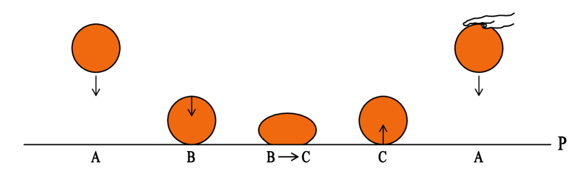
Figure 19: A suspension bridge is like a bouncing ball.

The ball is falling down until it reaches the position tangent to the plane as in position $B$. Then there is some positive time where the ball touches $P$; the reason is that it is squeezed and deformed, although probably less than illustrated in the $B\to C$ picture. But, of course, a very soft ball may have an important deformation. Just after the impact, the ball stores elastic energy which is hardly visible. After some time, the ball recovers its initial spherical shape and is ready to bounce up, see position $C$. When it is back in position $A$ it may store further energy, for instance with a hand pushing it downwards. For these reasons, we believe that there is some resemblance between bouncing balls and oscillating bridges.

5.3 Oscillating modes in suspension bridges: seeking the correct boundary conditions

Smith-Vincent [98, Section I.2] analyse the different forms of motion of a suspension bridge and write

The natural modes of vibration of a suspension bridge can be classified as vertical and torsional. In pure vertical modes all points on a given cross section move vertically the same amount and in phase… The amount of this vertical motion varies along the longitudinal axis of the bridge as a modified sine curve.

Then, concerning torsional motions, they write

In pure torsional modes each cross section rotates about an axis which is parallel to the longitudinal axis of the bridge and is in the same vertical plane as the centerline of the roadway. Corresponding points on opposite sides of the centerline of the roadway move equal distances but in opposite directions.

Moreover, Smith-Vincent also analyse small oscillations:

For small torsional amplitudes the movement of any point is essentially vertical, and the wave form or variation of amplitude along a line parallel to the longitudinal centerline of the bridge … is the same as for a corresponding pure vertical mode.

With these remarks at hand, in this section we try to set up a reliable eigenvalue problem. We consider the roadway bridge as a long narrow rectangular thin plate, simply supported on its short sides. So, let $\Omega=(0,L)\times(-\ell,\ell)\subset\mathbb{R}^{2}$ where $L$ is the length of the bridge and $2\ell$ is its width; a realistic assumption is that $2\ell\ll L$.

As already mentioned in Section 3.1, the choice of the boundary conditions is delicate since it depends on the physical model considered. We first recall that the boundary conditions $u=\Delta u=0$ are the so-called Navier boundary conditions, see Figure 20 which is taken from [80, p.96].

Figure 20: First appearance of Navier boundary conditions.

On flat parts of the boundary where no curvature is present, they describe simply supported plates, see e.g. [45]. When $x_{1}$ is fixed, either $x_{1}=0$ or $x_{1}=L$, these conditions reduce to $u=u_{x_{1}x_{1}}=0$. And precisely on these two sides, the roadway $\Omega$ is assumed to be simply supported; this is uniformly accepted in any of the models we met. The delicate point is the determination of the boundary conditions on the other sides.

In order to get into the problem, we start by dealing with the linear Kirchhoff-Love theory described in Section 3.1. In view of (2), the energy of the vertical deformation $u$ of a rectangular plate $\Omega=(0,L)\times(-\ell,\ell)$ subject to a load $f=f(x_{1},x_{2})$ is given by

$$\mathbb{E}(u)=\int_{\Omega}\left(\frac{1}{2}\left(\Delta u\right)^{2}+(\sigma-1)\det(D^{2}u)-f\,u\right)\,dx_{1}dx_{2}$$ (38)

and the corresponding Euler-Lagrange equation reads $\Delta^{2}u=f$ in $\Omega$. For a fully simply supported plate, that is $u=u_{x_{1}x_{1}}=0$ on the vertical sides and $u=u_{x_{2}x_{2}}=0$ on the horizontal sides, this problem has been solved by Navier [80] in 1823, see also [67, Section 2.1]. But Cauchy [20] criticised the work by Navier by claiming that

… Navier … avait considéré deux espèces de forces produites, les unes par la dilatation ou la contraction, les autres par la flexion de ce même plan. … Il me parut que ces deux espèces de forces pouvaient être réduites à une seule… .

Did Cauchy already have in mind the difference/analogy between bending, stretching, and torsion? In any case, since the bridge is not a fully simply supported plate, different boundary conditions should be considered on the horizontal sides. The load problem on the rectangle $\Omega$ with only the vertical sides being simply supported was considered by Lévy [64], Zanaboni [111], and Nadai [78], see also [67, Section 2.2] for the analysis of different kinds of boundary conditions on the remaining two sides $x_{2}=\pm\ell$. Let us also mention the more recent monograph [103, Chapter 3] for a very clear description of bending of rectangular plates.

A first natural possibility is to consider the horizontal sides to be free. If no physical constraint is present on the horizontal sides, then the boundary conditions there become (see e.g. [103, (2.40)])

$$u_{x_{2}x_{2}}(x_{1},\pm\ell)+\sigma u_{x_{1}x_{1}}(x_{1},\pm\ell)=0\,,\quad u_{x_{2}x_{2}x_{2}}(x_{1},\pm\ell)+(2-\sigma)u_{x_{1}x_{1}x_{2}}(x_{1},\pm\ell)=0\,,\quad x_{1}\in(0,L)\,.$$

Unfortunately, some physical constraints are present on the two horizontal sides, both because of the action of the hangers and because the cross section of the bridge may be considered to be rigid. Our purpose is to describe the oscillating modes of the plate $\Omega$ under the most possible realistic boundary conditions; we suggest here some new conditions to be required on the horizontal sides $x_{2}=\pm\ell$. Hopefully, they should allow to emphasise both vertical and torsional oscillations.

First of all, note that if the cross section of the roadway is rigid and behaves as in Figure 12 then each cross section has constant deflection from horizontal, that is, it rotates around its barycenter $B$: Prof. Farquharson, the man escaping in [116], ran following the middle line of the roadway precisely in order to avoid torsional oscillations. Denoting by $u=u(x_{1},x_{2})$ the vertical displacement of the roadway, this amounts to say that

$$u_{x_{2}}(x_{1},x_{2},t)=\Psi(x_{1},t)\qquad(x\in\Omega\,,\ t>0)$$ (39)

for some $\Psi$. If we translate this constraint on the vertical sides $x_{2}=\pm\ell$ of the plate $\Omega$, we obtain

$$\begin{array}[]{cc}u_{x_{2}x_{2}}(x_{1},x_{2})=0\quad x\in(0,L)\times\{-\ell,\ell\}\,,\\ 2\ell u_{x_{2}}(x_{1},-\ell)=2\ell u_{x_{2}}(x_{1},\ell)=u(x_{1},\ell)-u(x_{1},-\ell)\quad x_{1}\in(0,L)\,.\end{array}$$

Indeed, by (39) we have $u_{x_{2}x_{2}}\equiv 0$ in $\Omega$, which justifies both these conditions. Taking all the above boundary conditions into account, we are led to consider the following eigenvalue problem

$$\left\{\begin{array}[]{ll}\Delta^{2}u=\lambda u&x=(x_{1},x_{2})\in\Omega\,,\\ u(x_{1},x_{2})=u_{x_{1}x_{1}}(x_{1},x_{2})=0&x\in\{0,L\}\times(-\ell,\ell)\,,\\ u_{x_{2}x_{2}}(x_{1},x_{2})=0&x\in(0,L)\times\{-\ell,\ell\}\,,\\ 2\ell u_{x_{2}}(x_{1},-\ell)=2\ell u_{x_{2}}(x_{1},\ell)=u(x_{1},\ell)-u(x_{1},-\ell)&x_{1}\in(0,L)\,.\end{array}\right.$$ (40)

This is a nonlocal problem which combines boundary conditions on different parts of $\partial\Omega$. The oscillating modes of $\Omega$ are the eigenfunctions to (40). By separating variables, we find the two families of eigenfunctions

$$\sin\left(\frac{m\pi}{L}x_{1}\right)\ ,\qquad x_{2}\sin\left(\frac{m\pi}{L}x_{1}\right)\qquad(m\in\mathbb{N}\setminus\{0\})\ .$$ (41)

The first family describes pure vertical oscillations whereas the second family describes pure torsional oscillations with no vertical displacement of the middle line of the roadway. For fixed $m$, both these eigenfunctions correspond to the eigenvalue

$$\lambda_{m}=\frac{m^{4}\pi^{4}}{L^{4}}\ .$$

Although the “interesting” eigenfunctions to (40) are the ones in (41), further eigenfunctions might exist and are expected to have the form

$$\psi_{m}(x_{2})\,\sin\left(\frac{m\pi}{L}x_{1}\right)\qquad(m\in\mathbb{N}\setminus\{0\})$$ (42)

for some $\psi_{m}\in C^{4}(-\ell,ell)$ satisfying a suitable linear fourth order ODE, see [39].

Problem 21.

Determine all the eigenvalues and eigenfunctions to (40). Is $\lambda=0$ an eigenvalue? Which subspace of $H^{2}(\Omega)$ is spanned by these eigenfunctions? $\Box$

It would be interesting to find out if the corresponding loaded plate problem has an equilibrium.

Problem 22.

For any $f\in L^{2}(\Omega)$ study existence and uniqueness of a function $u\in H^{4}(\Omega)$ satisfying $\Delta^{2}u=f$ in $\Omega$ and (40)₂-(40)₃-(40)₄. Try first some particular forms of $f$ as in [67, Sections 2.2, 2.2.2] and then general $f=f(x_{1},x_{2})$. Is there any reasonable weak formulation for this problem? $\Box$

Problem (40) may turn out to be quite complicated from a mathematical point of view: it is not a variational problem and standard elliptic regularity does not apply. So, let us suggest an alternative model which seems to fit slightly better in well-known frameworks and also admits (41) as eigenfunctions. Consider the eigenvalue problem

$$\left\{\begin{array}[]{ll}\Delta^{2}u=\lambda u&x=(x_{1},x_{2})\in\Omega\,,\\ u(x_{1},x_{2})=u_{x_{1}x_{1}}(x_{1},x_{2})=0&x\in\{0,L\}\times(-\ell,\ell)\,,\\ u_{x_{2}x_{2}}(x_{1},x_{2})=u_{x_{2}x_{2}x_{2}}(x_{1},x_{2})=0&x\in(0,L)\times\{-\ell,\ell\}\,.\end{array}\right.$$ (43)

Here, the condition on the third normal derivative replaces (40)₄. This condition somehow “forces $u_{x_{2}x_{2}}$ to remain zero” which is precisely what happens in the bridge. It is straightforward to verify that (41) are eigenfunctions to (43) so that similar problems arise.

Problem 23.

Determine all the eigenvalues and eigenfunctions to (43). Which subspace of $H^{2}(\Omega)$ is spanned by these eigenfunctions? For any $f\in L^{2}(\Omega)$ study existence and uniqueness of a function $u\in H^{4}(\Omega)$ satisfying $\Delta^{2}u=f$ in $\Omega$ and (43)₂-(43)₃. $\Box$

A further alternative eigenvalue problem is also of some interest. A possible additional simplification in the model would be to assume that

$$u(x_{1},0,t)\simeq 0\qquad\mbox{for all }x_{1}\in(0,L)\,,\ t>0\,,$$ (44)

namely that the center line of the roadway has small vertical oscillations. If on one hand this seems realistic in view of [116], on the other hand this would preclude the appearance of wide vertical oscillations on the center line. In the whole, we believe that, qualitatively, the behavior of the plate will not change too much. By assuming (39) and that equality holds in (44), for all $x_{1}\in(0,L)$ and $t>0$ we obtain

$$u_{x_{2}}(x_{1},-\ell,t)=u_{x_{2}}(x_{1},\ell,t)=\frac{u(x_{1},\ell,t)-u(x_{1},-\ell,t)}{2\ell}\ ,\quad u(x_{1},\ell,t)=-u(x_{1},-\ell,t)\,.$$

By putting these together and decoupling equations on $x_{2}=\pm\ell$ we arrive at the Robin conditions

$$\ell u_{x_{2}}(x_{1},-\ell,t)+u(x_{1},-\ell,t)=0\,,\ \ell u_{x_{2}}(x_{1},\ell,t)-u(x_{1},\ell,t)=0\quad(x_{1}\in(0,L)\,,\ t>0)\,.$$

We believe that these boundary conditions may help to obtain oscillation properties also of the solutions to equations derived without assuming (44).

Problem 24.

Determine the eigenvalues $\lambda$ and the properties of the eigenfunctions to the following problem

$$\left\{\begin{array}[]{ll}\Delta^{2}u=\lambda u&x\in\Omega\,,\\ u(x_{1},x_{2})=u_{x_{1}x_{1}}(x_{1},x_{2})=0&(x_{1},x_{2})\in\{0,L\}\times(-\ell,\ell)\,,\\ u_{x_{2}x_{2}}(x_{1},x_{2})=0&(x_{1},x_{2})\in(0,L)\times\{-\ell,\ell\}\,,\\ \ell u_{x_{2}}(x_{1},-\ell)+u(x_{1},-\ell)=0&x_{1}\in(0,L)\,,\\ \ell u_{x_{2}}(x_{1},\ell)-u(x_{1},\ell)=0&x_{1}\in(0,L)\,.\\ \end{array}\right.$$

This would give an idea of what kind of oscillations should be expected in the below model equation (54). $\Box$

In this section we set up several eigenvalue problems for thin rectangular plates simply supported on two opposite sides. There is no evidence on which could be the best boundary conditions on the remaining sides. Once these are determined, it could be of great interest to have both theoretical and numerical information on the the behavior of eigenvalues and eigenfunctions. The conditions should be sought in order to perfectly describe the oscillating modes of suspension bridges. In a work in preparation [39] we tackle these problems.

5.4 Seeking the critical energy threshold

The title of this section should not deceive. We will not give a precise method how to determine the energy threshold which gives rise to torsional oscillations in a plate. We do have an idea how to proceed but several steps are necessary before reaching the final goal.

Consider the plate $\Omega=(0,L)\times(-\ell,\ell)$ and the incomplete eigenvalue problem

$$\left\{\begin{array}[]{ll}\Delta^{2}u=\lambda u&x\in\Omega\,,\\ u(x_{1},x_{2})=u_{x_{1}x_{1}}(x_{1},x_{2})=0&(x_{1},x_{2})\in\{0,L\}\times(-\ell,\ell)\,.\end{array}\right.$$ (45)

Problem incomplete lacks conditions on the remaining sided $x_{2}=\pm\ell$ and, as mentioned in the previous section, it is not clear which boundary conditions should be added there.

In order to explain which could be the method to determine the critical energy threshold, consider the simple case where the plate is square, $\Omega=(0,\pi)\times(-\frac{\pi}{2},\frac{\pi}{2})$, and let us complete (45) with the “simplest” boundary conditions, namely the Navier boundary conditions which represent a fully simply supported plate. As already mentioned these are certainly not the correct boundary conditions for a bridge but they are quite helpful to describe the method we are going to suggest. For different and more realistic boundary conditions, we refer to the paper in preparation [39]. So, consider the problem

$$\left\{\begin{array}[]{ll}\Delta^{2}u=\lambda u&x\in\Omega\,,\\ u(x_{1},x_{2})=u_{x_{1}x_{1}}(x_{1},x_{2})=0&(x_{1},x_{2})\in\{0,\pi\}\times(-\frac{\pi}{2},\frac{\pi}{2})\,,\\ u(x_{1},x_{2})=u_{x_{2}x_{2}}(x_{1},x_{2})=0&(x_{1},x_{2})\in(0,\pi)\times\{-\frac{\pi}{2},\frac{\pi}{2}\}\ .\end{array}\right.$$ (46)

It is readily seen that, for instance, $\lambda=625$ is an eigenvalue for (46) and that there are 4 linearly independent corresponding eigenfunctions

$$\{\sin(24x_{1})\cos(7x_{2}),\,\sin(20x_{1})\cos(15x_{2}),\,\sin(15x_{1})\cos(20x_{2}),\,\sin(7x_{1})\cos(24x_{2})\}\ .$$ (47)

It is well-known that similar facts hold for the second order eigenvalue problem $-\Delta u=\lambda u$ on the square, so what we are discussing is not surprising. What we want to emphasise here is that, associated to the same eigenvalue $\lambda=625$, we have 4 different kinds of vibrations in the $x_{1}$-direction and each one of these vibrations has its own counterpart in the $x_{2}$-direction corresponding to torsional oscillations. We believe that this will be true for any boundary conditions on $x_{2}=\pm\ell$ completing (45) and for any values of $L$ and $\ell$. We refer again to Figure 3 for the patterns of some vibrating plates.

Consider now a general plate $\Omega=(0,L)\times(-\ell,\ell)$ and let $f\in L^{2}(\Omega)$; in view of [67, Section 2.2], we expect the solution to the problem

$$\left\{\begin{array}[]{ll}\Delta^{2}u=f&x\in\Omega\,,\\ u(x_{1},x_{2})=u_{x_{1}x_{1}}(x_{1},x_{2})=0&(x_{1},x_{2})\in\{0,\pi\}\times(-\frac{\pi}{2},\frac{\pi}{2})\,,\\ \mbox{other boundary conditions}&(x_{1},x_{2})\in(0,\pi)\times\{-\frac{\pi}{2},\frac{\pi}{2}\}\ ,\end{array}\right.$$ (48)

to be of the kind

$$u(x_{1},x_{2})=\sum_{m=1}^{\infty}\psi_{m}(x_{2})\sin\left(\frac{m\pi}{L}x_{1}\right)\qquad(x_{1},x_{2})\in\Omega$$

for some functions $\psi_{m}$ depending on the Fourier coefficients of $f$. Since we have in mind small $\ell$, we can formally expand $\psi_{m}$ in Taylor polynomials and obtain

$$\psi_{m}(x_{2})=\psi_{m}(0)+\psi_{m}^{\prime}(0)x_{2}+o(x_{2})\qquad\mbox{as }x_{2}\to 0\ .$$

Hence, $u$ may approximately be written as a combination of the functions in (41):

$$u(x_{1},x_{2})\approx\sum_{m=1}^{\infty}[a_{m}+b_{m}x_{2}]\sin\left(\frac{m\pi}{L}x_{1}\right)\qquad(x_{1},x_{2})\in\Omega$$

where $a_{m}=\psi_{m}(0)$ and $b_{m}=\psi^{\prime}_{m}(0)$. If instead of a stationary problem such as (48), $u=u(x_{1},x_{2},t)$ satisfies an evolution problem with the same boundary conditions, then also its coefficients depend on time:

$$u(x_{1},x_{2},t)\approx\sum_{m=1}^{\infty}\Big{(}a_{m}(t)+b_{m}(t)x_{2}\Big{)}\sin\left(\frac{m\pi}{L}x_{1}\right)\qquad(x_{1},x_{2})\in\Omega\,,\ t>0\ .$$ (49)

Let now ${\cal E}(t)$ denote the instantaneous total energy of the bridge, as determined in (37). What follows is not precise, it is a qualitative attempt to describe combined vertical and torsional oscillations. In particular, due to the restoring cables and hangers, the sine functions in (49) should be modified in order to display different behaviors for positive and negative arguments. Moreover, we call “small” any quantity which is less than unity and “almost zero” (in symbols $\cong 0$) any quantity which has a smaller order of magnitude when compared with small quantities. Finally, in order to avoid delicate sign arguments, we will often refer to $a_{m}^{2}$ and $b_{m}^{2}$ instead of $a_{m}$ and $b_{m}$.

$\bullet$ Small energy. As long as ${\cal E}(t)$ is small one may not even see oscillations, but if somebody stands on the bridge he might be able to feel oscillations. For instance, standing on the sidewalk of a bridge, one can feel the oscillations created by a car going through the roadway but the oscillations will not be visible to somebody watching the roadway from a point outside the bridge. For small energies ${\cal E}(t)$ only small oscillations appear and the corresponding solution (49) has small coefficients $a_{m}(t)$ while $b_{m}(t)\cong 0$. More precisely,

$$\left\{\begin{array}[]{ll}\forall\varepsilon>0\ \exists\delta>0\quad\mbox{such that}\quad{\cal E}(t)<\delta\ \Longrightarrow\ a_{m}(t)^{2}<\varepsilon\ \forall m\,,\\ \exists\gamma>0\quad\mbox{such that}\quad{\cal E}(t)<\gamma\ \Longrightarrow\ b_{m}(t)\cong 0\ \forall m\,.\end{array}\right.$$ (50)

The reason of the second of (50) is that even small variations of the $b_{m}$’s correspond to a large variation of the total energy ${\cal E}$ because the huge masses of the cross sections would rotate along the large length $L$ of the roadway. On the other hand, the first of (50) may be strengthened by assuming that also some of the $a_{m}$’s are almost zero for small ${\cal E}$; in particular, we expect that this happens for large $m$ since these coefficients correspond to higher eigenvalues

$$\forall\overline{m}\in\mathbb{N}\setminus\{0\}\quad\exists{\cal E}_{\overline{m}}>0\quad\mbox{such that}\quad{\cal E}(t)<{\cal E}_{\overline{m}}\ \Longrightarrow\ a_{m}(t)\cong 0\quad\forall m>\overline{m}\ .$$ (51)

To better understand this point, let us compute the elongation $\Gamma_{m}$ due to the $m$-th mode:

$$\Gamma_{m}(t):=\int_{0}^{L}\bigg{(}\sqrt{1+\frac{m^{2}\pi^{2}}{L^{2}}\,a_{m}(t)^{2}\,\cos^{2}\left(\frac{m\pi}{L}x_{1}\right)}\,-\,1\bigg{)}\,dx_{1}\ ;$$ (52)

this describes the stretching elastic energy since it is the difference between the length of the roadway deformed by one single mode and the length of the roadway at rest. Due to the coefficient $\frac{m^{2}\pi^{2}}{L^{2}}$, it is clear that if $a_{m}^{2}\equiv a_{m+1}^{2}$ then $\Gamma_{m}(t)<\Gamma_{m+1}(t)$. This is the reason why (51) holds.

$\bullet$ Increasing energy. According to (51), as long as ${\cal E}(t)<{\cal E}_{\overline{m}}$ one has $a_{m}(t)\cong 0$ for all $m>\overline{m}$. If ${\cal E}(t)$ increases but remains smaller than ${\cal E}_{\overline{m}}$, then the coefficients $a_{m}(t)^{2}$ for $m=1,...,\overline{m}$ also increase. But they cannot increase to infinity since (52) implies that the length of the roadway would also increase to infinity. So, when the total energy ${\cal E}(t)$ reaches the threshold ${\cal E}_{\overline{m}}$ the superlinear elastic structure of the bridge forces the solution (49) to add one mode, so that $a_{\overline{m}+1}(t)\not\cong 0$. Hence, the number of modes $\not\cong 0$ is a nondecreasing function of ${\cal E}$.

$\bullet$ Critical energy threshold. What is described above is purely theoretical, but the bridge has several physical constraints. Of course, it cannot be stretched to infinity, it will break down much before. In particular, the number of active modes cannot increase to infinity. The elastic properties of the bridge determine a critical (maximal) number of possible active modes, say $\mu$. If the energy is distributed on the $\mu$ coefficients $a_{1}$,…,$a_{\mu}$, and if it increases up to ${\cal E}_{\mu}$, once again the superlinear elastic structure of the bridge forces the solution (49) to change mode, but this time from the $a_{m}$ to the $b_{m}$; due to (52), further stretching of the roadway would require much more energy than switching oscillations on torsional modes. The switch is due to an impulse caused by the instantaneous stopping of the falling roadway imposed by the sustaining cables and the elongated hangers. And which torsional modes will be activated depends on which coupled modes have the same eigenvalue; as an example, consider (47) which, roughly speaking, says that the motion may change from $24$ to $7$ oscillations in the $x_{1}$-direction with a consequent change of oscillation also in the $x_{2}$-direction.

$\bullet$ Summarising… Let $u$ in (49) describe the vertical displacement of the roadway. The bridge has several characteristic values which depend on its elastic structure.

$\diamondsuit$ An integer number $\mu\in\mathbb{N}$ such that $a_{m}(t)\cong 0$ and $b_{m}(t)\cong 0$ for all $m>\mu$, independently of the value of ${\cal E}(t)$.

$\diamondsuit$ $\mu$ different energy “increasing modes thresholds” $E_{1},...,E_{\mu}$.

$\diamondsuit$ The critical energy threshold $\overline{E}=E_{\mu}$.

Assume that ${\cal E}(0)=0$, in which case $u(x_{1},x_{2},0)=0$, and that $t\mapsto{\cal E}(t)$ is increasing. As long as ${\cal E}(t)\leq E_{1}$ we have $a_{m}\cong 0$ for all $m\geq 2$ and $b_{m}\cong 0$ for all $m\geq 1$; moreover, $t\mapsto a_{1}(t)^{2}$ is increasing. When ${\cal E}(t)$ reaches and exceeds $E_{1}$ there is a first switch: the function $a_{2}^{2}$ starts being positive while, as long as ${\cal E}(t)\leq E_{2}$, we still have $a_{m}\cong 0$ for all $m\geq 3$ and $b_{m}\cong 0$ for all $m\geq 1$. And so on, until ${\cal E}(t)=E_{\mu}=\overline{E}$. At this point, also because of an impulse, the energy forces the solution to have a nonzero coefficient $b_{1}$ rather than a nonzero coefficient $a_{\mu+1}$. The impulse forces $u$ to lower the number of modes for which $a_{m}\not\cong 0$. For instance, the observation by Farquharson (The motion, which a moment before had involved nine or ten waves, had shifted to two) quoted in Section 2 shows that, for the Tacoma Bridge, there was a change such as

$$\Big{(}a_{m}\cong 0\ \forall m\geq 11,\ b_{m}\cong 0\ \forall m\geq 1\Big{)}\ \longrightarrow\ \Big{(}a_{m}\cong 0\ \forall m\geq 3,\ b_{m}\cong 0\ \forall m\geq 2\Big{)}\ .$$ (53)

In order to complete the material in this section, two major problems are still to be solved.

- Find the correct boundary conditions on $x_{2}=\pm\ell$.

- Find at which energy levels the “transfer of energy between modes” occurs, see (53).

Both these problems are addressed in a forthcoming paper [39].

6 Conclusions and future perspectives

So far, we observed phenomena displayed by real structures, we discussed models, and we recalled some theoretical results. In this section we take advantage from all this work, we summarise all the phenomena and remarks previously discussed, and we reach several conclusions.

6.1 A new mathematical model for suspension bridges

We suggest here a new mathematical model for the description of oscillations in suspension bridges. We expect the solution to the corresponding equation to display both self-excited oscillations and instantaneous switch between vertical and torsional oscillations. Moreover, the critical energy threshold (corresponding to the flutter speed) appears in the equation.

Let $\Omega=(0,L)\times(-\ell,\ell)\subset\mathbb{R}^{2}$ where $L$ represents the length of the bridge and $2\ell$ represents the width of the roadway. Assume that $2\ell\ll L$ and consider the initial-boundary value problem

$$\left\{\begin{array}[]{ll}u_{tt}+\Delta^{2}u+\delta u_{t}+f(u)=\varphi(x,t)&x=(x_{1},x_{2})\in\Omega,\ t>0,\\ u(x_{1},x_{2},t)=u_{x_{1}x_{1}}(x_{1},x_{2},t)=0&x\in\{0,L\}\times(-\ell,\ell),\ t>0,\\ u_{x_{2}x_{2}}(x_{1},x_{2},t)=0&x\in(0,L)\times\{-\ell,\ell\},\ t>0,\\ u_{x_{2}}(x_{1},-\ell,t)=u_{x_{2}}(x_{1},\ell,t)&x_{1}\in(0,L),\ t>0,\\ u_{t}(x_{1},-\ell,t)+u(x_{1},-\ell,t)=E(t)\,[u_{t}(x_{1},\ell,t)+u(x_{1},\ell,t)]&x_{1}\in(0,L),\ t>0,\\ u(x,0)=u_{0}(x)&x\in\Omega,\\ u_{t}(x,0)=u_{1}(x)&x\in\Omega.\end{array}\right.$$ (54)

Here, $u=u(x,t)$ represents the vertical displacement of the plate, $u_{0}(x)$ is its initial position while $u_{1}(x)$ is its initial vertical velocity. Before discussing the other terms and conditions, let us remark that if one wishes to have smooth solutions, a compatibility condition between boundary and initial conditions is needed:

$$u_{1}(x_{1},-\ell)+u_{0}(x_{1},-\ell)=E(0)\,[u_{1}(x_{1},\ell)+u_{0}(x_{1},\ell)]\qquad\forall x_{1}\in(0,L)\ .$$ (55)

The function $\varphi$ represents an external source, such as the wind, which is responsible for the variation of the total energy ${\cal E}(t)$ inserted in the structure which, in turn, can be determined by

$${\cal E}(t)=\int_{\Omega}\varphi(x,t)^{2}\,dx\ .$$ (56)

Of course, it is much simpler to compute ${\cal E}(t)$ in terms of the known source $\varphi$ rather than in terms of the unknown solution $u$ and its derivatives. The function $E$ is then defined by

$$E(t)=\left\{\begin{array}[]{ll}1&\mbox{if }{\cal E}(t)\leq\overline{E}\\ -1&\mbox{if }{\cal E}(t)>\overline{E}\end{array}\right.$$ (57)

where $\overline{E}>0$ is the critical energy threshold defined in Section 5.2; hence, the function $E(t)$ is a discontinuous nonlocal term which switches to $\pm 1$ according to whether the total energy is smaller/larger than the critical threshold. So, (54)₅ is a dynamic boundary condition involving the total energy of the bridge. When ${\cal E}(t)\leq\overline{E}$ there is no torsional energy $E_{t}$ and the motion tends to become of pure vertical-type, that is, with $u_{x_{2}}\cong 0$: to see this, note that in this case (54)₅ may be written as

$$\frac{\partial}{\partial t}\Big{\{}[u(x_{1},\ell,t)-u(x_{1},-\ell,t)]e^{t}\Big{\}}=0\qquad\forall x_{1}\in(0,L)\ .$$

This means that as long as ${\cal E}(t)\leq\overline{E}$, the map $t\mapsto|u(x_{1},\ell,t)-u(x_{1},-\ell,t)|$ decreases so that the two opposite endpoints of any cross section tend to have the same vertical displacement and to move synchronously as in a pure vertical motion. When ${\cal E}(t)>\overline{E}$ condition (54)₅ may be written as

$$\frac{\partial}{\partial t}\Big{\{}[u(x_{1},\ell,t)+u(x_{1},-\ell,t)]e^{t}\Big{\}}=0\qquad\forall x_{1}\in(0,L)\ .$$

This means that as long as ${\cal E}(t)>\overline{E}$, the map $t\mapsto|u(x_{1},\ell,t)+u(x_{1},-\ell,t)|$ decreases so that the two opposite endpoints of any cross section tend to have zero average and to move asynchronously as in a pure torsional motion, that is, with $u(x_{1},0,t)\cong\frac{1}{2}[u(x_{1},\ell,t)+u(x_{1},-\ell,t)]\cong 0$.

Note that in (54) the jump of $E(t)$ from/to $\pm 1$ occurs simultaneously and instantaneously along all the points located on the sides of the roadway; hence, either all or none of the cross sections have some torsional motion, in agreement with what has been observed for the Tacoma Bridge, see [5] and also [97, pp.50-51]. The form (56) and the switching criterion for $E(t)$ in (57) mean that problem (54) models a situation where if a gust of wind is sufficiently strong then, instantaneously, a torsional motion appears. One could also consider the case where

$${\cal E}(t)\simeq\int_{0}^{t}\int_{\Omega}\varphi(x,\tau)^{2}\,dx\,d\tau\$$

which would model a situation where if the wind blows for too long then at some critical time, instantaneously, a torsional motion appears. However, the problem with (56) is much simpler because it is local in time.

The differential operator in (54) is derived according to the linear Kirchhoff-Love model for a thin plate, see Section 3.1. We have neglected a strong distinction between the bending and stretching elastic energies which are, however, quite different in long narrow plates, see [67, Section 8.3] and previous work by Cox [26]; if one wishes to make some corrections, one should add a further nonlinear term $g(\nabla u,D^{2}u)$ and the equation would become quasilinear, see Problem 29. But, as already mentioned in Section 3.1, we follow here a compromise and merely consider a semilinear problem. Concerning the nonlinearity $f(u)$, some superlinearity should be required. For instance, $f(u)=u+\varepsilon u^{3}$ with $\varepsilon>0$ small could be a possible choice; alternatively, one could take $f(u)=a(e^{bu}-1)$ as in [72] for some $a,b>0$. In the first case the hangers are sought as ideal springs and gravity is somehow neglected, in the second case more relevance is given to gravity and to the possibility of slackening hangers. Finally, $\delta u_{t}$ is a damping term which represents the positive structural damping of the structure; its role should be to weaken the effect of the nonlinear term $f(u)$, see Problem 27.

As far as we are aware, there is no standard theory for problems like (54). It is a nonlocal problem since it links behaviors on different parts of the boundary and involves the function $E(t)$ in (57). It also has dynamic boundary conditions which are usually delicate to handle.

Problem 25.

Prove that if $\varphi(x,t)\equiv 0$ then (54) only admits the trivial solution $u\equiv 0$. The standard trick of multiplying the equation in (54) by $u$ or $u_{t}$ and integrating over $\Omega$ does not allow to get rid of all the boundary terms. Note that, in this case, $E(t)\equiv 1$. $\Box$

Problem 26.

Study existence and uniqueness results for (54); prove continuous dependence results with respect to the data $\varphi$, $u_{0}$, $u_{1}$, and with respect to possible perturbations of $f$. Of course, the delicate conditions to deal with are (54)₄ and (54)₅. If problem (54) were ill-posed, what must be changed in order to have a well-posed problem? $\Box$

Problem 27.

Study (54) with no damping, that is, $\delta=0$: does the solution display oscillations such as (17) when $t$ tends to some finite blow up instant? Then study the competition between the damping term $\delta u_{t}$ and the self-exciting term $f(u)$: for a given $f$ is it true that if $\delta$ is sufficiently large then the solution $u$ is global in time? We believe that the answer is negative and that the only effect of the damping term is to delay the blow up time. $\Box$

Problem 28.

Determine the regularity of the solutions $u$ to (54) and study the importance of the compatibility condition (55). $\Box$

Problem 29.

Insert into the equation (54) a correction term for the elastic energies, something like

$$g(\nabla u,D^{2}u)=-\left(\frac{u_{x_{1}}}{\sqrt{1+u_{x_{1}}^{2}}}\right)_{x_{1}}-\gamma\left(\frac{u_{x_{1}}}{\sqrt{1+u_{x_{1}}^{2}}}\right)_{x_{2}}$$

with $\gamma>0$ small. Then prove existence, uniqueness and continuous dependence results. $\Box$

An important tool to study (54) would be the eigenvalues and eigenfunctions of the corresponding stationary problem. In view of the dynamic boundary conditions (54)₅, a slightly simpler model could be considered, see (40) or (43) and subsequent discussion in Section 5.3. We have no feeling on what could be the better choice…

6.2 A possible explanation of the Tacoma collapse

Hopefully, this paper sheds some further light on oscillating bridges. We have emphasised the necessity of models fulfilling the requirements of (GP) since, otherwise, the solution will not display the phenomena visible in real bridges. In particular, any equation aiming to model the complex behavior of bridges should contain information on at least two possible kinds of oscillations: this target may be achieved either by considering a PDE, or by considering coupled systems of ODE’s, or by linking the two oscillations within a unique function solving a suitable ODE. A further contribution of this paper is the remark that there might be some hidden elastic energy in the bridge and that there is no simple way to detect it. Not only this energy is larger than the kinetic and potential energy but also it may give rise, almost instantaneously, to self-excited oscillations.

We now put together all these observations in order to afford an explanation of the Tacoma collapse. As we shall see, our explanation turns out to agree with all of them.

On November 7, 1940, for some time before 10:00 AM, the bridge was oscillating as it did many other times before. The wind was apparently more violent than usual and, moreover, it continued for a long time. The oscillations of the bridge were completely similar to those displayed in the interval $(0,80)$ of the plot in Figure 14. Since the energy involved was quite large, also the oscillations were quite large. The roadway was far from its equilibrium position and, consequently, the restoring force due to the sustaining cables and to the hangers did not obey ${\cal LHL}$. The oscillations were governed by a fairly complicated differential equation such as (54) which, however, may be approximated by (16) after assuming (15), since this equation possesses the main features of many fourth order differential equations, both ODE’s and PDE’s. It is not clear which superlinear function $f$ would better describe the restoring nonlinear elastic forces, but any function $f=f(s)$ asymptotically linear as $s\to 0$ and superlinear as $|s|\to\infty$ generates the same qualitative behavior of solutions, see Theorem 6. As the wind was keeping on blowing, the total energy ${\cal E}$ in the bridge was increasing; the bridge started ruminating energy and, in particular, its stored elastic energy $E_{\ell}$ was also increasing. Unfortunately, nobody knew how to measure $E_{\ell}$ because, otherwise, (22) would have taught in some advance that sudden wider vertical oscillations and subsequent torsional oscillations would have appeared. After each cycle, when the cross section of the bridge violently reached position $B$ in Figure 17, a delta Dirac mass increased the internal elastic energy $E_{\ell}$. As the wind was continuously blowing, after some cycles the elastic energy became larger than the critical energy threshold $\overline{E}$ of the bridge, see Section 5.2. This threshold may be computed provided one knows the elastic structure of the bridge, see Section 5.4. As soon as $E_{\ell}>\overline{E}$, the function $E(t)$ in (57) switched from $+1$ to $-1$, a torsional elastic energy $E_{t}$ appeared and gave rise, almost instantaneously, to a torsional motion. As described in (53), due to the impulse, the energy switched to the first torsional mode $b_{1}$ rather than to a further vertical mode $a_{11}$; so, the impulse forced $u$ to lower the number of modes for which $a_{m}\not\cong 0$ and the motion, which a moment before had involved nine or ten waves, shifted to two. At that moment, the graph of the function $w=w(t)$, describing the bridge according to (15), reached time $t=95$ in the plot in Figure 14. Oscillations immediately went out of control and after some more oscillations the bridge collapsed.

One should compare this description with the original one from the Report [5], see also [34, pp.26-29] and [97, Chapter 4].

6.3 What about future bridges?

Equation (16) is a simple prototype equation for the description of self-excited oscillations. None of the previously existing mathematical models ever displayed this phenomenon which is also visible in oscillating bridges. The reason is not that the behavior of the bridge is too complicated to be described by a differential equation but mainly because they fail to satisfy (GP); this prevents the appearance of oscillations and therefore the projects based on the corresponding equation may contain huge errors. In order to avoid bad surprises as in the past, many projects nowadays include stiffening trusses or strong dampers. This has the great advantage to maintain the bridge much closer to its equilibrium position and to justify ${\cal LHL}$. But this also has disadvantages, see [57]. First of all, they create an artificial stiffness which can give rise to the appearances of cracks in the more elastic structure of the bridge. Second, damping effects and stiffening trusses significantly increase the weight and the cost of the whole structure. Moreover, in extreme conditions, they may become useless: under huge external solicitations the bridge would again be too far from its equilibrium position and would violate ${\cal LHL}$. So, hopefully, one should find alternative solutions, see again [57].

One can act both on the structure and on the model. In order to increase the flutter speed, some suggestions on how to modify the design were made by Rocard [90, pp.169-173]: he suggests how to modify the components of the bridge in order to raise the right hand side of (36). More recently, some attempts to improve bridges performances can be found in [52] where, in particular, a careful analysis of the role played by the hangers is made. But much work has still to be done; from [52, p.1624], we quote

Research on the robustness of suspension bridges is at the very beginning.

From a theoretical point of view, one should first determine a suitable equation satisfying (GP). Our own suggestion is to consider (54) where one should choose a reliable nonlinearity $f$ and add coefficients to the other terms, according to the expected technical features of the final version of the bridge: its length, its width, its weight, the materials used for the construction, the expected external solicitations, the structural damping… Since we believe that the solution to this equation may display blow up, which means a strong instability, a crucial role is played by all the constants which appear in the equation. Hence, a careful measurement of these parameters is necessary. Moreover, a sensitivity analysis for the continuous dependence of the solution on the parameters should be performed. Once the most reliable nonlinearity and parameters are chosen, the so obtained equation should be tested numerically to see if the solution displays dangerous phenomena. In particular, one should try to estimate, at least numerically, the critical energy threshold and the possible blow up time. Also purely theoretical estimates are of great interest; in general, these are difficult to obtain but even if they are not very precise they can be of some help.

In a “perfect model” for a suspension bridge, one should also take into account the role of the sustaining cables and of the towers. Each cable links all the hangers on the same side of the bridge, its shape is a catenary of given length and the hangers cannot all elongate at the same time. The towers link the two cables and, in turn, all the hangers on both sides of the roadway. Cables and towers are further elastic components of the structure which, of course, modify considerably the model, its oscillating modes, its total elastic energy, etc. In this paper we have not introduced these components but, in the next future, this would be desirable.

An analysis of the more flexible parts of the roadway should also be performed; basically, this consists in measuring the “instantaneous local energy” defined by

$${\bf E}(u(t),\omega)=\int_{\omega}\left[\left(\frac{|\Delta u(t)|^{2}}{2}+(\sigma-1)\det(D^{2}u(t))\right)+\frac{u_{t}(t)^{2}}{2}+F(u(t))\right]\,dx_{1}dx_{2}$$ (58)

for solutions $u=u(t)$ to (54), for any $t\in(0,T)$, and for any subregion $\omega\subset\Omega$ of given area. In (58) we recognize the first term to be as in the Kirchhoff-Love model, see (2); moreover, $F(s)=\int_{0}^{s}f(\sigma)d\sigma$.

Problem 30.

Let $\Omega=(0,L)\times(-\ell,\ell)$, consider problem (54) and let $u=u(t)$ denote its solution provided it exists and is unique, see Problem 26. For given lengths $a<L$ and $b<2\ell$ consider the set $\Re$ of rectangles entirely contained in $\Omega$ and whose sides have lengths $a$ (horizontal) and $b$ (vertical). Let ${\bf E}$ be as in (58) and consider the maximisation problem

$$\max_{\omega\in\Re}\ {\bf E}(u(t),\omega)\ .$$

Using standard tools from calculus of variations, prove that there exists an optimal rectangle and study its dependence on $t\in(0,T)$; the natural conjecture is that, at least as $t\to T$, it is the “middle rectangle” $(\frac{L-a}{2},\frac{L+a}{2})\times(-\frac{b}{2},\frac{b}{2})$. Then one should find out if there exists some optimal ratio $a/b$. Finally, it would be extremely useful to find the dependence of the energy ${\bf E}(u(t),\omega)$ on the measure $ab$ of the rectangle $\omega$; this would allow to minimise costs for reinforcing the plate. We do not expect analytical tools to be able to locate optimal rectangles nor to give exact answers to the above problems so that a good numerical procedure could be of great help. $\Box$

In [98, Chapter IV] an attempt to estimate the impact of stiffening trusses is made, although only one kind of truss design is considered. In order to determine the best way to display the truss, one should solve the following simplified problems from calculus of variations. A first step is to consider the linear model.

Problem 31.

Assume that the rectangular plate $\Omega=(0,L)\times(-\ell,\ell)$ is simply supported on all its sides and that it is submitted to a constant load $f\equiv 1$. In the linear theory by Kirchhoff-Love model, see (38), its elastic energy is given by

$$E_{0}(\Omega)=\ -\min_{u\in H^{2}\cap H^{1}_{0}(\Omega)}\ \int_{\Omega}\left(\frac{1}{2}\left(\Delta u\right)^{2}+(\sigma-1)\det(D^{2}u)-u\right)\,dx_{1}dx_{2}\ .$$

Here, $H^{2}\cap H^{1}_{0}(\Omega)$ denotes the usual Hilbertian Sobolev space which, since we are in the plane, is embedded into $C^{0,\alpha}(\overline{\Omega})$. The unique minimiser $u$ solves the corresponding Euler-Lagrange equation which reads

$$\Delta^{2}u=1\mbox{ in }\Omega\,,\quad u=\Delta u=0\mbox{ on }\partial\Omega$$

and which may be reduced to a system involving the torsional rigidity of $\Omega$:

$$-\Delta u=v\,,\ -\Delta v=1\mbox{ in }\Omega\,,\quad u=v=0\mbox{ on }\partial\Omega\,.$$

Let $\lambda>0$ and denote by $\Gamma_{\lambda}$ the set of connected curves $\gamma$ contained in $\overline{\Omega}$, such that $\gamma\cap\partial\Omega\neq\emptyset$, and whose length is $\lambda$: the curves $\gamma$ represent the stiffening truss to be put below the roadway. For any $\gamma\in\Gamma_{\lambda}$ the elastic energy of the reinforced plate $\Omega\setminus\gamma$ is given by

$$E_{\gamma}(\Omega)=\ -\min_{u\in H^{2}\cap H^{1}_{0}(\Omega\setminus\gamma)}\ \int_{\Omega}\left(\frac{1}{2}\left(\Delta u\right)^{2}+(\sigma-1)\det(D^{2}u)-u\right)\,dx_{1}dx_{2}\ ,$$

and this energy should be minimised among all possible $\gamma\in\Gamma_{\lambda}$:

$$\min_{\gamma\in\Gamma_{\lambda}}\ E_{\gamma}(\Omega)\ .$$

Is there an optimal $\gamma_{\lambda}$ for any $\lambda>0$? When we asked this question to Buttazzo [18] and Santambrogio [93], we received positive answers; their optimism is justified by the connectedness assumption and by their previous work [19, 94] which also gives hints on how the line $\gamma_{\lambda}$ should look like. In fact, for a realistic model, one should further require that all the endpoints of $\gamma_{\lambda}$ lie on the boundary $\partial\Omega$. Finally, since the stiffening truss has a cost $C>0$ per unit length, one should also solve the minimisation problem

$$\min_{\lambda\geq 0}\ \left\{C\lambda+\min_{\gamma\in\Gamma_{\lambda}}\ E_{\gamma}(\Omega)\right\}\,;$$

if $C$ is sufficiently small, we believe that the minimum exists. $\Box$

Problem 31 is just a simplified version of the “true problem” which… should be completed!

Problem 32.

Let $\Omega=(0,L)\times(-\ell,\ell)$ and fix some $\lambda>0$. Denote by $\Gamma_{\lambda}$ the set of connected curves contained in $\overline{\Omega}$ whose length is $\lambda$ and whose endpoints belong to $\partial\Omega$. Study the minimisation problem

$$\min_{\gamma\in\Gamma_{\lambda}}\ \left|\min_{u\in{\mathcal{H}}(\Omega\setminus\gamma)}\ \int_{\Omega}\left(\frac{1}{2}\left(\Delta u\right)^{2}+(\sigma-1)\det(D^{2}u)-u\right)\,dx_{1}dx_{2}\right|\ ,$$

where

$${\mathcal{H}}(\Omega\setminus\gamma)=\{u\in H^{2}(\Omega\setminus\gamma);\ \mbox{(\ref{eigen2})${}_{2}$ holds},\ \mbox{+ something on }x_{2}=\pm\ell\mbox{ and on }\gamma\}\ .$$

First of all, instead of “something”, one should find the correct conditions on $x_{2}=\pm\ell$ and on $\gamma$. This could also suggest to modify the energy function to be minimised with an additional boundary integral. The questions are similar. Is there an optimal $\gamma_{\lambda}$ for any $\lambda>0$? Is there an optimal $\lambda>0$ if one also takes into account the cost? $\Box$

Then one should try to solve the same problems with variable loads.

Problem 33.

Solve Problems 31 and 32 with nonconstant loads $f\in L^{2}(\Omega)$, so that the minimum problem becomes

$$\min_{\gamma\in\Gamma_{\lambda}}\ \left|\min_{u\in{\mathcal{H}}(\Omega\setminus\gamma)}\ \int_{\Omega}\left(\frac{1}{2}\left(\Delta u\right)^{2}+(\sigma-1)\det(D^{2}u)-\,fu\right)\,dx_{1}dx_{2}\right|\ .$$

What happens if $f\not\in L^{2}(\Omega)$? For instance, if $f$ is a delta Dirac mass concentrated at some point $x_{0}\in\Omega$. $\Box$

Acknowledgment. The author is grateful to his colleague Pier Giorgio Malerba, a structural engineer at the Politecnico of Milan, for several interesting and stimulating discussions.

References

- [1] A.M. Abdel-Ghaffar, Suspension bridge vibration: continuum formulation, J. Eng. Mech. 108, 1215-1232 (1982)
- [2] N.U. Ahmed, H. Harbi, Mathematical analysis of dynamic models of suspension bridges, SIAM J. Appl. Math. 58, 853-874 (1998)
- [3] B. Akesson, Understanding bridges collapses, CRC Press, Taylor & Francis Group, London (2008)
- [4] O.H. Ammann, Additional stiffening of Bronx-Whitestone Bridge, Civil Engineering, March (1946)
- [5] O.H. Ammann, T. von Kármán, G.B. Woodruff, The failure of the Tacoma Narrows Bridge, Federal Works Agency, 1941
- [6] Anonymous, Stays and brakes check oscillation of Whitestone Bridge, Engineering News-Record, December 5 (1940)
- [7] S.S. Antman, Ordinary differential equations of nonlinear elasticity. I. Foundations of the theories of nonlinearly elastic rods and shells, Arch. Rat. Mech. Anal. 61, 307-351 (1976)
- [8] S.S. Antman, Buckled states of nonlinearly elastic plates, Arch. Rat. Mech. Anal. 67, 111-149 (1978)
- [9] J.M. Ball, Convexity conditions and existence theorems in nonlinear elasticity, Arch. Rat. Mech. Anal. 63, 337-403 (1977)
- [10] V. Benci, D. Fortunato, Existence of solitons in the nonlinear beam equation, J. Fixed Point Theory Appl. 11, 261-278 (2012)
- [11] C. Bender, Historical sketch of the successive improvements in suspension bridges to the present time, American Soc. Civil Eng. Vol. I, 27-43 (1872)
- [12] E. Berchio, A. Ferrero, F. Gazzola, P. Karageorgis, Qualitative behavior of global solutions to some nonlinear fourth order differential equations, J. Diff. Eq. 251, 2696-2727 (2011)
- [13] F. Bleich, Dynamic instability of truss-stiffened suspension bridges under wind action, Proceedings ASCE 74, 1269-1314 (1948)
- [14] F. Bleich, C.B. McCullough, R. Rosecrans, G.S. Vincent, The Mathematical theory of vibration in suspension bridges, U.S. Dept. of Commerce, Bureau of Public Roads, Washington D.C. (1950)
- [15] J. Bodgi, S. Erlicher, P. Argoul, Lateral vibration of footbridges under crowd-loading: continuous crowd modeling approach, Key Engineering Materials 347, 685-690 (2007)
- [16] J.M.W. Brownjohn, Observations on non-linear dynamic characteristics of suspension bridges, Earthquake Engineering & Structural Dynamics 23, 1351-1367 (1994)
- [17] D. Bruno, V. Colotti, F. Greco, P. Lonetti, A parametric deformability analysis of long span bridge schemes under moving loads, IABMAS04, International Conference on Bridge Maintenance, Safety and Management, 735-737, Kyoto (2004)
- [18] G. Buttazzo, private discussion held at the conference on New trends in shape optimization, Pisa (2012)
- [19] G. Buttazzo, E. Oudet, E. Stepanov, Optimal transportation problems with free Dirichlet regions, In: Variational methods for discontinuous structures, Cernobbio 2001, Progress in Nonlinear Differential Equations 51, 41-65, Birkhäuser Verlag, Basel (2002)
- [20] A. Cauchy, Recherches sur l’équilibre et le mouvement intérieur des corps solides ou fluides, élastiques ou non élastiques, Bulletin des Science de la Société Philomathique de Paris, 9-13 (1823)
- [21] Y. Chen, P.J. McKenna, Traveling waves in a nonlinearly suspended beam: theoretical results and numerical observations, J. Diff. Eq. 136, 325-355 (1997)
- [22] E. Chladni, Entdeckungen über die theorie des klanges, Weidmanns Erben und Reich, Leipzig (1787)
- [23] P.G. Ciarlet, Mathematical elasticity. Vol.II, Theory of plates, Studies in Mathematics and its Applications 27, North-Holland Publishing Co. Amsterdam (1997)
- [24] M. Como, Stabilità aerodinamica dei ponti di grande luce. Introduzione all’ingegneria strutturale, E. Giangreco, Torino, UTET (2002)
- [25] M. Como, S. Del Ferraro, A. Grimaldi, A parametric analysis of the flutter instability for long span suspension bridges, Wind and Structures 8, 1-12 (2005)
- [26] H.L. Cox, Buckling of thin plates in compression, Aero. Res. Council Rep. & Memor. 1554, H.M.S.O. (1933)
- [27] L. D’Ambrosio, E. Mitidieri, Entire solutions of certain fourth order elliptic problems and related inequalities, preprint
- [28] P. Destuynder, M. Salaun, Mathematical analysis of thin plate models, Mathématiques & Applications 24, Springer-Verlag, Berlin (1996)
- [29] G. Diana, private discussion held at the IABMAS12 conference, Stresa (2012)
- [30] P. Drábek, G. Holubová, A. Matas, P. Nečesal, Nonlinear models of suspension bridges: discussion of the results, Appl. Math. 48, 497-514 (2003)
-
[31]
Encyclopedia Britannica, Academic Edition,
http://www.britannica.com/EBchecked/topic/271336/Hookes-law -
[32]
English Russia, No more dancing for the bridge in Volgograd?,
http://englishrussia.com/2012/01/18/no-more-dancing-for-the-bridge-in-volgograd/ - [33] F.B. Farquharson, Letter to the Editor, ENR, p.37, July 3 (1941)
- [34] F.B. Farquharson, Aerodynamic stability of suspension bridges: with special reference to the Tacoma Narrows Bridge, Part I: Investigations prior to October 1941, Investigation conducted by the Structural Research Laboratory, University of Washington - Seattle: University of Washington Press (1949)
- [35] F.B. Farquharson, Aerodynamic stability of suspension bridges: with special reference to the Tacoma Narrows Bridge, Part III: The Investigation of the original Tacoma Narrows Bridge, Investigation conducted by the Structural Research Laboratory, University of Washington - Seattle: University of Washington Press (1952)
- [36] F.B. Farquharson, Aerodynamic stability of suspension bridges: with special reference to the Tacoma Narrows Bridge, Part IV: Model investigations which influence the design of the new Tacoma Narrows Bridge, Investigation conducted by the Structural Research Laboratory, University of Washington - Seattle: University of Washington Press (1954)
- [37] L. Fazzo, Traballa il ponte di Assago: spavento dopo il concerto, il Giornale.it, 26 Feb. 2011, http://www.ilgiornale.it/milano/traballa-ponte-assago-spavento-dopo-concerto/26-02-2011/articolo-id=508454
- [38] G.R. Fernandes, G.J. Denipotti, D.H. Konda, A BEM formulation for analysing the coupled stretching-bending problems of plates reinforced by rectangular beams with columns defined in the domain, Comput. Mech. 45, 523-539 (2010)
- [39] A. Ferrero, F. Gazzola, in preparation
- [40] A. Ferrero, F. Gazzola, H.-Ch. Grunau, Decay and eventual local positivity for biharmonic parabolic equations, Disc. Cont. Dynam. Syst. 21, 1129-1157 (2008)
- [41] L. Franck, P. Lestuzzi, A. Low, Synchronous lateral excitation of footbridges, Swiss Federal Institute of Technology, IMAC-EPFL Lausanne (2009)
- [42] K. Friedrichs, Die randwert und eigenwertprobleme aus der theorie der elastischen platten (anwendung der direkten methoden der variationsrechnung), Math. Ann. 98, 205-247 (1927)
- [43] F. Gazzola, H.-Ch. Grunau, Radial entire solutions for supercritical biharmonic equations, Math. Ann. 334, 905-936 (2006)
- [44] F. Gazzola, H.-Ch. Grunau, Eventual local positivity for a biharmonic heat equation in , Disc. Cont. Dynam. Syst. S 1, 83-87 (2008)
- [45] F. Gazzola, H.-Ch. Grunau, G. Sweers, Polyharmonic boundary value problems, LNM 1991, Springer (2010)
- [46] F. Gazzola, R. Pavani, Blow up oscillating solutions to some nonlinear fourth order differential equations, Nonlinear Analysis 74, 6696-6711 (2011)
- [47] F. Gazzola, R. Pavani, Blow-up oscillating solutions to some nonlinear fourth order differential equations describing oscillations of suspension bridges, IABMAS12, International Conference on Bridge Maintenance, Safety, Management, Resilience and Sustainability, 3089-3093, Stresa 2012, Biondini & Frangopol (Editors), Taylor & Francis Group, London (2012)
- [48] F. Gazzola, R. Pavani, Wide oscillations finite time blow up for solutions to nonlinear fourth order differential equations, Arch. Rat. Mech. Anal. 207, 717-752 (2013)
- [49] H. Goldstein, C. Poole, J. Safko, Classical mechanics, 3rd Edition, Addison Wesley (2002)
- [50] D. Green, W.G. Unruh, Tacoma Bridge failure - a physical model, Amer. J. Physics 74, 706-716 (2006)
- [51] M.E. Gurtin, On the nonlinear theory of elasticity, In: Contemporary developments in continuum mechanics and partial differential equations, 237-253, G.M. de la Penha & L.A. Medeiros (Editors), North-Holland, Amsterdam (1978)
- [52] M. Haberland, S. Hass, U. Starossek, Robustness assessment of suspension bridges, IABMAS12, International Conference on Bridge Maintenance, Safety, Management, Resilience and Sustainability, 1617-1624, Stresa 2012, Biondini & Frangopol (Editors), Taylor & Francis Group, London (2012)
- [53] S. Hao, I-35W Bridge collapse, J. Bridge Eng. 15, 608-614 (2010)
- [54] M. Hayden, The book of bridges, Galahad Books, New York, 1976
- [55] IABMAS 2012 ( International Conference on Bridge Maintenance, Safety and Management), Stresa 2012, http://www.iabmas2012.org/
-
[56]
D. Imhof, Bridge failure database, University of Cambridge,
http://www.bridgeforum.org/dir/collapse/type/ - [57] T. Kawada, History of the modern suspension bridge: solving the dilemma between economy and stiffness, ASCE Press (2010)
- [58] T. Kawada, A. Hirai, Additional mass method - A new approach to suspension bridge rehabilitation, Official Proceedings, 2nd Annual International Bridge Conference, Engineers Society of Western Pennsylvania, Pittsburgh (1985)
- [59] G.R. Kirchhoff, Über das gleichgewicht und die bewegung einer elastischen scheibe, J. Reine Angew. Math. 40, 51-88 (1850)
- [60] W. Lacarbonara, Nonlinear structural mechanics, Springer (2013)
- [61] W. Lacarbonara, V. Colone, Dynamic response of arch bridges traversed by high-speed trains, J. Sound and Vibration 304, 72-90 (2007)
- [62] A.C. Lazer, P.J. McKenna, Large scale oscillatory behaviour in loaded asymmetric systems, Ann. Inst. H. Poincaré Anal. non Lin. 4, 243-274 (1987)
- [63] A.C. Lazer, P.J. McKenna, Large-amplitude periodic oscillations in suspension bridges: some new connections with nonlinear analysis, SIAM Rev. 32, 537-578 (1990)
- [64] M. Lévy, Sur l’équilibre élastique d’une plaque rectangulaire, Comptes Rendus Acad. Sci. Paris 129, 535-539 (1899)
- [65] A.E.H. Love, A Treatise on the mathematical theory of elasticity, 4th edition, Cambridge Univ. Press (1927)
- [66] J.H.G. Macdonald, Lateral excitation of bridges by balancing pedestrians, Proceedings of the Royal Society A, Mathematical, Physical & Engineering Sciences 465, 1055-1073 (2009)
- [67] E.H. Mansfield, The bending and stretching of plates, 2nd edition, Cambridge Univ. Press (2005) (first edition in 1964)
- [68] A. Matas, J. Očenášek, Modelling of suspension bridges, Proceedings of Computational Mechanics 2, 275-278 (2002)
- [69] P.J. McKenna, Torsional oscillations in suspension bridges revisited: fixing an old approximation, Amer. Math. Monthly 106, 1-18 (1999)
- [70] P.J. McKenna, Large-amplitude periodic oscillations in simple and complex mechanical systems: outgrowths from nonlinear analysis, Milan J. Math. 74, 79-115 (2006)
- [71] P.J. McKenna, K.S. Moore, The global structure of periodic solutions to a suspension bridge mechanical model, IMA J. Appl. Math. 67, 459-478 (2002)
- [72] P.J. McKenna, C.Ó Tuama, Large torsional oscillations in suspension bridges visited again: vertical forcing creates torsional response, Amer. Math. Monthly 108, 738-745 (2001)
- [73] P.J. McKenna, W. Walter, Nonlinear oscillations in a suspension bridge, Arch. Rat. Mech. Anal. 98, 167-177 (1987)
- [74] P.J. McKenna, W. Walter, Travelling waves in a suspension bridge, SIAM J. Appl. Math. 50, 703-715 (1990)
- [75] J. Melan, Theory of arches and suspension bridges, Myron Clark Publ. Comp. (1913)
- [76] R. Mindlin, Influence of rotatory inertia and shear on flexural motions of isotropic elastic plates, J. Appl. Mech. 18, 31-38 (1951)
- [77] B. Moran, A bridge that didn’t collapse, American Heritage of Invention and Technology 15, 10-18 (1999)
- [78] A. Nadai, Die elastischen platten, Springer-Verlag, Berlin (1968) (first edition in 1925)
- [79] P.M. Naghdi, The theory of shells and plates, In: Handbuch der Physik 6a/2, 425-640, S. Flügge & C. Truesdell (Editors), Springer, Berlin (1972)
- [80] C.L. Navier, Extraits des recherches sur la flexion des plans élastiques, Bulletin des Science de la Société Philomathique de Paris, 92-102 (1823)
- [81] C.L. Navier, Mémoire sur les ponts suspendus, Imprimerie Royale, Paris (1823)
- [82] E.L. Pavlo, Widening and stiffening Whitestone Bridge, Engineering News-Record, October 2 (1947)
- [83] C. Pearson, N. Delatte, Collapse of the Quebec Bridge, 1907, J. Perform. Constr. Facil. 20, 84-91 (2006)
- [84] L.A. Peletier, W.C. Troy, Spatial patterns. Higher order models in physics and mechanics. Progress in Nonlinear Differential Equations and their Applications, 45, Birkhäuser Boston Inc. (2001)
-
[85]
B. Perks, The Golden Gateway, pictures and story,
http://pcimagenetwork.com/golden-gate/golden-gate.html - [86] W.A. Provis, Observations on the effect of wind on the suspension bridge over Menai Strait, Minutes of Proceedings of the Institution of Civil Engineers 1, 74-77 (1841)
- [87] W. Reid, A short account of the failure of a part of the Brighton Chain Pier, in the gale of the 30th of November 1836, Papers on Subjects Connected with the Duties of the Corps of Royal Engineers (Professional Papers of the Corps of Royal Engineers), Vol. I (1844)
- [88] E. Reissner, On the theory of bending elastic plates, J. Math. and Phys. 23, 184-191 (1944)
- [89] E. Reissner, The effect of transverse shear deformations on the bending of elastic plates, J. Appl. Mech. 12, 69-77 (1945)
- [90] Y. Rocard, Dynamic instability: automobiles, aircraft, suspension bridges, Crosby Lockwood, London (1957)
- [91] J.S. Russell, On the vibration of suspension bridges and other structures; and the means of preventing injury from this cause, Transactions of the Royal Scottish Society of Arts, Vol.1 (1841)
- [92] K. Sanderson, Millennium bridge wobble explained, Nature, Published online 17 December 2008, doi:10.1038/news.2008.1311
- [93] F. Santambrogio, private discussion held at the conference on New trends in shape optimization, Pisa (2012)
- [94] F. Santambrogio, P. Tilli, Blow-up of optimal sets in the irrigation problem, J. Geom. Anal. 15, 343-362 (2005)
- [95] R.H. Scanlan, Developments in low-speed aeroelasticity in the civil engineering field, AIAA Journal 20, 839-844 (1982)
- [96] R.H. Scanlan, J.J. Tomko, Airfoil and bridge deck flutter derivatives, J. Eng. Mech. 97, 1717-1737 (1971)
- [97] R. Scott, In the wake of Tacoma. Suspension bridges and the quest for aerodynamic stability, ASCE Press (2001)
- [98] F.C. Smith, G.S. Vincent, Aerodynamic stability of suspension bridges: with special reference to the Tacoma Narrows Bridge, Part II: Mathematical analysis, Investigation conducted by the Structural Research Laboratory, University of Washington - Seattle: University of Washington Press (1950)
-
[99]
A. Stella, Assago, la passerella della paura smetterà di ballare, Corriere della Sera, 01 Marzo 2011,
http://milano.corriere.it/milano/notizie/cronaca/11-marzo-1/assago-passerella-ammortizzatore-oscillazioni-forum-190124249413.shtml - [100] S. Timoshenko, Theory of elasticity, McGraw-Hill, New York (1951) (first edition in 1934)
- [101] S. Timoshenko, W. Woinowsky-Krieger, Theory of plates and shells, McGraw-Hill, New York (1959)
- [102] C. Truesdell, Some challenges offered to analysis by rational thermomechanics, In: Contemporary developments in continuum mechanics and partial differential equations, 495-603, G.M. de la Penha & L.A. Medeiros (Editors), North-Holland, Amsterdam (1978)
- [103] E. Ventsel, T. Krauthammer, Thin plates and shells: theory, analysis, and applications, Marcel Dekker inc., New York (2001)
- [104] F. Verantius, Machinae novae, 1615
- [105] P. Villaggio, Mathematical models for elastic structures, Cambridge University Press, Cambridge (1997)
- [106] G.S. Vincent, Aerodynamic stability of suspension bridges: with special reference to the Tacoma Narrows Bridge, Part V: Extended studies: Logarithmic decrement field damping, Investigation conducted by the Structural Research Laboratory, University of Washington - Seattle: University of Washington Press (1954)
- [107] T. von Kármán, Feestigkeitsprobleme in maschinenbau, In: Encycl. der Mathematischen Wissenschaften, Vol. IV/4C, 348-352, F. Klein & C. Müller (Editors), Leipzig (1910)
- [108] R. Walther, B. Houriet, W. Isler, P. Moïa, J.-F. Klein, Cable stayed bridges, Thomas Telford Publishing, London, 2nd edition (1999)
- [109] K. Wardhana, F.C. Hadipriono, Analysis of recent bridge failures in the United States, J. Perform. Constr. Facil. 17, 144-150 (2003)
- [110] Y. Xiang, G. Tang, C. Liu, Cracking mechanism and simplified design method for bottom flange in prestressed concrete box girder bridge, J. Bridge Eng. 16, 267-274 (2011)
- [111] O. Zanaboni, Risoluzione, in serie semplice, della lastra rettangolare appoggiata, sottoposta all’azione di un carico concentrato comunque disposto, Annali Mat. Pura Appl. 19, 107-124 (1940)
- [112] S. Živanović, I.M. Díaz, A. Pavić, Influence of walking and standing crowds on structural dynamic properties, Proceedings of the IMAC-XXVII, Orlando 2009, Society for Experimental Mechanics Inc. VIDEOS
- [113] Assago Bridge oscillation, http://www.youtube.com/watch?v=C5V9ymTD3e4
- [114] Chladni experiment on vibrating membranes, http://www.youtube.com/watch?v=Qf0t4qIVWF4
- [115] London Millennium Bridge swaying, http://www.youtube.com/watch?v=eAXVa-XWZ8
- [116] Tacoma Narrows Bridge collapse, http://www.youtube.com/watch?v=3mclp9QmCGs
- [117] Volgograd Bridge oscillations, http://www.bbc.co.uk/news/10138398