Wormhole Hamiltonian Monte Carlo

Abstract

In machine learning and statistics, probabilistic inference involving multimodal distributions is quite difficult. This is especially true in high dimensional problems, where most existing algorithms cannot easily move from one mode to another. To address this issue, we propose a novel Bayesian inference approach based on Markov Chain Monte Carlo. Our method can effectively sample from multimodal distributions, especially when the dimension is high and the modes are isolated. To this end, it exploits and modifies the Riemannian geometric properties of the target distribution to create wormholes connecting modes in order to facilitate moving between them. Further, our proposed method uses the regeneration technique in order to adapt the algorithm by identifying new modes and updating the network of wormholes without affecting the stationary distribution. To find new modes, as opposed to rediscovering those previously identified, we employ a novel mode searching algorithm that explores a residual energy function obtained by subtracting an approximate Gaussian mixture density (based on previously discovered modes) from the target density function.

1 Introduction

In Bayesian inference, it is well known that standard Markov Chain Monte Carlo (MCMC) methods tend to fail when the target distribution is multimodal (Neal, 1993, 1996; Celeux et al., 2000; Neal, 2001; Rudoy and Wolfe, 2006; Sminchisescu and Welling, 2011; Craiu et al., 2009). These methods typically fail to move from one mode to another since such moves require passing through low probability regions. This is especially true for high dimensional problems with isolated modes. Therefore, despite recent advances in computational Bayesian methods, designing effective MCMC samplers for multimodal distribution has remained a major challenge. In the statistics and machine learning literature, many methods have been proposed address this issue (see for example, Neal, 1996, 2001; Warnes, 2001; Laskey and Myers, 2003; Hinton et al., 2004; Braak, 2006; Rudoy and Wolfe, 2006; Sminchisescu and Welling, 2011; Ahn et al., 2013) However, these methods tend to suffer from the curse of dimensionality (Hinton et al., 2004; Ahn et al., 2013).

In this paper, we propose a new algorithm, which exploits and modifies the Riemannian geometric properties of the target distribution to create wormholes connecting modes in order to facilitate moving between them. Our method can be regarded as an extension of Hamiltonian Monte Carlo (HMC). Compared to random walk Metropolis, standard HMC explores the target distribution more efficiently by exploiting its geometric properties. However, it too tends to fail when the target distribution is multimodal since the modes are separated by high energy barriers (low probability regions) (Sminchisescu and Welling, 2011).

In what follows, we provide an brief overview of HMC. Then, we introduce our method assuming that the locations of the modes are known (either exactly or approximately), possibly through some optimization techniques (e.g., (Kirkpatrick et al., 1983; Sminchisescu and Triggs, 2002)). Next, we relax this assumption by incorporating a mode searching algorithm in our method in order to identify new modes and to update the network of wormholes.

2 Preliminaries

Hamiltonian Monte Carlo (HMC) (Duane et al., 1987; Neal, 2010) is a Metropolis algorithm with proposals guided by Hamiltonian dynamics. HMC improves upon random walk Metropolis by proposing states that are distant from the current state, but nevertheless have a high probability of acceptance. These distant proposals are found by numerically simulating Hamiltonian dynamics, whose state space consists of its position, denoted by the vector $\boldsymbol{\theta}$, and its momentum, denoted by a vector $\boldsymbol{p}$. Our objective is to sample from the distribution of $\boldsymbol{\theta}$ with the probability density function (up to some constant) $\pi(\boldsymbol{\theta})$. We usually assume that the auxiliary momentum variable $\boldsymbol{p}$ has a multivariate normal distribution (the same dimension as $\boldsymbol{\theta}$) with mean zero. The covariance of $\boldsymbol{p}$ is usually referred to as the mass matrix, $\boldsymbol{M}$, which in standard HMC is usually set to the identity matrix, ${\boldsymbol{I}}$, for convenience.

Based on $\boldsymbol{\theta}$ and $\boldsymbol{p}$, we define the potential energy, $U(\boldsymbol{\theta})$, and the kinetic energy, $K(\boldsymbol{p})$. We set $U(\boldsymbol{\theta})$ to minus the log probability density of $\boldsymbol{\theta}$ (plus any constant). For the auxiliary momentum variable $\boldsymbol{p}$, we set $K(\boldsymbol{p})$ to be minus the log probability density of $\boldsymbol{p}$ (plus any constant). The Hamiltonian function is then defined as follows:

$$H(\boldsymbol{\theta},\boldsymbol{p}) = U(\boldsymbol{\theta})+K(\boldsymbol{p})$$

The partial derivatives of $H(\boldsymbol{\theta},\boldsymbol{p})$ determine how $\boldsymbol{\theta}$ and $\boldsymbol{p}$ change over time, according to Hamilton’s equations,

$$\begin{array}[]{lcrcr }\displaystyle\dot{\boldsymbol{\theta}}&=&\nabla_{\boldsymbol{p}}H({\boldsymbol{\theta}},{\boldsymbol{p}})&=&{\boldsymbol{M}}^{-1}{\boldsymbol{p}}\\[12.0pt] \displaystyle\dot{\boldsymbol{p}}&=&-\nabla_{\boldsymbol{\theta}}H({\boldsymbol{\theta}},{\boldsymbol{p}})&=&-\nabla_{\boldsymbol{\theta}}U(\boldsymbol{\theta})\end{array}$$ (2.3)

Note that ${\boldsymbol{M}}^{-1}{\boldsymbol{p}}$ can be interpreted as velocity.

In practice, solving Hamiltonian’s equations exactly is difficult, so we need to approximate these equations by discretizing time, using some small step size $e$. For this purpose, the leapfrog method is commonly used. We can use some number, $L$, of these leapfrog steps, with some stepsize, $e$, to propose a new state in the Metropolis algorithm. This proposal is either accepted or rejected based on the Metropolis acceptance probability.

While HMC explores the target distribution more efficiently than random walk Metropolis, it does not fully exploits its geometric properties. Recently, Girolami and Calderhead (2011) proposed a new method, called Riemannian Manifold HMC (RMHMC), that improvs the efficiency of standard HMC by automatically adapting to the local structure. To this end, they follow Amari and Nagaoka (2000) and propose Hamiltonian Monte Carlo methods defined on the Riemannian manifold endowed with metric ${\boldsymbol{G}}_{0}({\boldsymbol{\theta}})$, which is set to the Fisher information matrix. More specifically, they define Hamiltonian dynamics in terms of a position-specific mass matrix, $\boldsymbol{M}$, set to ${\boldsymbol{G}}_{0}({\boldsymbol{\theta}})$. The standard HMC method is a special case of RMHMC with ${\boldsymbol{G}}_{0}({\boldsymbol{\theta}})={\boldsymbol{I}}$. Here, we use the notation ${\boldsymbol{G}}_{0}$ to generally refer to a Riemannian metric, which is not necessarily the Fisher information. In the following section, we introduce a natural modification of ${\boldsymbol{G}}_{0}$ such that the associated Hamiltonian dynamical system has a much greater chance of moving between isolated modes.

3 Wormhole Hamiltonian Monte Carlo

Consider a manifold $\mathcal{M}$ endowed with a generic metric ${\boldsymbol{G}}_{0}({\boldsymbol{\theta}})$. Given a differentiable curve $\boldsymbol{\theta}(t):[0,T]\to\mathcal{M}$ one can define the arclength along this curve as

$$\ell({\boldsymbol{\theta}}):=\int_{0}^{T}\sqrt{\dot{\boldsymbol{\theta}}(t)^{\textsf{T}}{\boldsymbol{G}}_{0}({\boldsymbol{\theta}}(t))\dot{\boldsymbol{\theta}}(t)}dt$$ (3.1)

Under very general geometric assumptions, which are nearly always satisfied in statistical models, given any two points ${\boldsymbol{\theta}}_{1},{\boldsymbol{\theta}}_{2}\in\mathcal{M}$ there exists a curve ${\boldsymbol{\theta}}(t):[0,T]\to\mathcal{M}$ satisfying the boundary conditions ${\boldsymbol{\theta}}(0)={\boldsymbol{\theta}}_{1},{\boldsymbol{\theta}}(T)={\boldsymbol{\theta}}_{2}$ whose arclength is minimal among such curves. The length of such a minimal curve defines a distance function on $\mathcal{M}$. In Euclidean space, where ${\boldsymbol{G}}_{0}({\boldsymbol{\theta}})\equiv{\boldsymbol{I}}$, the shortest curve connecting ${\boldsymbol{\theta}}_{1}$ and ${\boldsymbol{\theta}}_{2}$ is simply a straight line with the Euclidean length $\|{\boldsymbol{\theta}}_{1}-{\boldsymbol{\theta}}_{2}\|_{2}$.

As mentioned above, while standard HMC algorithms explore the target distribution more efficiently, they nevertheless fail to move between isolated modes since these modes are separated by high energy barriers (Sminchisescu and Welling, 2011). To address this issue, we propose to replace the base metric ${\boldsymbol{G}}_{0}$ with a new metric for which the distance between modes is shortened. This way, we can facilitate moving between modes by creating “wormholes” between them.

Let $\hat{\boldsymbol{\theta}}_{1}$ and $\hat{\boldsymbol{\theta}}_{2}$ be two modes of the target distribution. We define a straight line segment, ${\boldsymbol{v}}_{W}:=\hat{\boldsymbol{\theta}}_{2}-\hat{\boldsymbol{\theta}}_{1}$, and refer to a small neighborhood (tube) of the line segment as a wormhole. Next, we define a wormhole metric, ${\boldsymbol{G}_{W}}({\boldsymbol{\theta}})$, in the vicinity of the wormhole. The metric ${\boldsymbol{G}_{W}}({\boldsymbol{\theta}})$ is an inner product assigning a non-negative real number to a pair of tangent vectors ${\boldsymbol{u}},{\boldsymbol{w}}$: ${\boldsymbol{G}_{W}}({\boldsymbol{\theta}})({\boldsymbol{u}},{\boldsymbol{w}})\in\mathbb{R}^{+}$. To shorten the distance in the direction of ${\boldsymbol{v}}_{W}$, we project both ${\boldsymbol{u}},{\boldsymbol{w}}$ to the plane normal to ${\boldsymbol{v}}_{W}$ and then take the Euclidean inner product of those projected vectors. We set ${\boldsymbol{v}}_{W}^{*}={\boldsymbol{v}}_{W}/\|{\boldsymbol{v}}_{W}\|$ and define a pseudo wormhole metric ${\boldsymbol{G}^{*}_{W}}$ as follows:

$${\boldsymbol{G}^{*}_{W}}({\boldsymbol{u}},{\boldsymbol{w}}) := \langle{\boldsymbol{u}}-\langle{\boldsymbol{u}},{\boldsymbol{v}}_{W}^{*}\rangle{\boldsymbol{v}}_{W}^{*},{\boldsymbol{w}}-\langle{\boldsymbol{w}},{\boldsymbol{v}}_{W}^{*}\rangle{\boldsymbol{v}}_{W}^{*}\rangle$$

$$= {\boldsymbol{u}}^{\textsf{T}}[{\boldsymbol{I}}-{\boldsymbol{v}}_{W}^{*}({\boldsymbol{v}}_{W}^{*})^{\textsf{T}}]{\boldsymbol{w}}$$

Note that ${\boldsymbol{G}^{*}_{W}}:={\boldsymbol{I}}-{\boldsymbol{v}}_{W}^{*}({\boldsymbol{v}}_{W}^{*})^{\textsf{T}}$ is semi-positive definite (degenerate at ${\boldsymbol{v}}_{W}^{*}\neq 0$). We modify this metric to make it positive definite, and define the wormhole metric ${\boldsymbol{G}_{W}}$ as follows:

$${\boldsymbol{G}_{W}}={\boldsymbol{G}^{*}_{W}}+\varepsilon{\boldsymbol{v}}_{W}^{*}({\boldsymbol{v}}_{W}^{*})^{\textsf{T}}={\boldsymbol{I}}-(1-\varepsilon){\boldsymbol{v}}_{W}^{*}({\boldsymbol{v}}_{W}^{*})^{\textsf{T}}$$ (3.2)

where $0<\varepsilon\ll 1$ is a small positive number.

To see that the wormhole metric ${\boldsymbol{G}_{W}}$ in fact shortens the distance between $\hat{\boldsymbol{\theta}}_{1}$ and $\hat{\boldsymbol{\theta}}_{2}$, consider a simple case where ${\boldsymbol{\theta}}(t)$ follows a straight line: ${\boldsymbol{\theta}}(t)={\boldsymbol{\theta}}_{1}+{\boldsymbol{v}}_{W}t,t\in[0,1]$. In this case, the distance under ${\boldsymbol{G}_{W}}$ is

$$\mathrm{dist}(\hat{\boldsymbol{\theta}}_{1},\hat{\boldsymbol{\theta}}_{2})=\int_{0}^{1}\sqrt{{\boldsymbol{v}}_{W}^{\textsf{T}}{\boldsymbol{G}_{W}}{\boldsymbol{v}}_{W}}dt=\sqrt{\varepsilon}\|{\boldsymbol{v}}_{W}\|\ll\|{\boldsymbol{v}}_{W}\|$$

which is much smaller than the Euclidean distance.

Next, we define the overall metric, $\boldsymbol{G}$, for the whole parameter space of $\boldsymbol{\theta}$ as a weighted sum of the base metric ${\boldsymbol{G}_{0}}$ and the wormhole metric ${\boldsymbol{G}_{W}}$,

$${\boldsymbol{G}}({\boldsymbol{\theta}})=(1-\mathfrak{m}({\boldsymbol{\theta}})){\boldsymbol{G}_{0}}({\boldsymbol{\theta}})+\mathfrak{m}({\boldsymbol{\theta}}){\boldsymbol{G}_{W}}$$ (3.3)

where $\mathfrak{m}({\boldsymbol{\theta}})\in(0,1)$ is a mollifying function designed to make the wormhole metric ${\boldsymbol{G}_{W}}$ influential in the vicinity of the wormhole only. In this paper, we choose the following mollifier:

$$\mathfrak{m}({\boldsymbol{\theta}}):=\exp\{-(\|{\boldsymbol{\theta}}-\hat{\boldsymbol{\theta}}_{1}\|+\|{\boldsymbol{\theta}}-\hat{\boldsymbol{\theta}}_{2}\|-\|\hat{\boldsymbol{\theta}}_{1}-\hat{\boldsymbol{\theta}}_{2}\|)/F\}$$ (3.4)

where the influence factor $F>0$, is a free parameter that can be tuned to modify the extent of the influence of ${\boldsymbol{G}_{W}}$: decreasing $F$ makes the influence of ${\boldsymbol{G}_{W}}$ more restricted around the wormhole. The resulting metric leaves the base metric almost intact outside of the wormhole, while making the transition of the metric from outside to inside smooth. Within the wormhole, the trajectories are mainly guided in the wormhole direction ${\boldsymbol{v}}_{W}^{*}$: ${\boldsymbol{G}}({\boldsymbol{\theta}})\approx{\boldsymbol{G}_{W}}$, so ${\boldsymbol{G}}({\boldsymbol{\theta}})^{-1}\approx{\boldsymbol{G}_{W}}^{-1}$ has the dominant eigen-vector ${\boldsymbol{v}}_{W}^{*}$ (with eigen-value $1/\varepsilon\gg 1$), thereafter ${\boldsymbol{v}}\sim\mathcal{N}({\bf 0},{\boldsymbol{G}}({\boldsymbol{\theta}})^{-1})$ tends to be directed in ${\boldsymbol{v}}_{W}^{*}$.

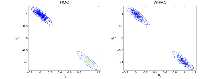
Figure 1: Comparing HMC and WHMC in terms of sampling from a two-dimensional posterior distribution with two isolated modes.

We use the modified metric (3.3) in RMHMC and refer to the resulting algorithm as Wormhole Hamiltonian Monte Carlo (WHMC). Figure 1 compares WHMC to standard HMC based on the following illustrative example appeared in the paper by Welling and Teh (2011):

$$\theta_{d} \sim \mathcal{N}(\theta_{d},\sigma_{d}^{2}),\quad d=1,2.$$

$$x_{i} \sim \frac{1}{2}\mathcal{N}(\theta_{1},\sigma_{x}^{2})+\frac{1}{2}\mathcal{N}(\theta_{1}+\theta_{2},\sigma_{x}^{2}).$$

Here, we set $\theta_{1}=0,\theta_{2}=1,\sigma_{1}^{2}=10,\sigma_{2}^{2}=1$, $\sigma_{x}^{2}=2$, and generate 1000 data points from the above model. In Figure 1, the dots show the posterior samples of $(\theta_{1},\theta_{2})$ given the simulated data. While HMC is trapped in one mode, WHMC moves easily between the two modes. For this example, we set ${\boldsymbol{G}_{0}}=\boldsymbol{I}$ to make WHMC comparable to standard HMC. Further, we use $0.03$ and $0.3$ for $\varepsilon$ and $F$ respectively.

For more than two modes, we can construct a network of wormholes by connecting any two modes with a wormhole. Alternatively, we can create a wormhole between neighboring modes only. In this paper, we define the neighborhood using a minimal spanning tree (Kleinberg and Tardos, 2005).

The above method could suffer from two potential shortcomings in higher dimensions. First, the effect of wormhole metric could diminish fast as the sampler leaves one mode towards another mode. Second, such mechanism, which modifies the dynamics in the existing parameter space, could interfere with the native HMC dynamics in the neighborhood of a wormhole.

To address the first issue, we add an external vector field to enforce the movement between modes. More specifically, we define a vector field, ${\boldsymbol{f}}({\boldsymbol{\theta}},{\boldsymbol{v}})$, in terms of the position parameter $\boldsymbol{\theta}$ and the velocity vector ${\boldsymbol{v}}={\boldsymbol{G}}({\boldsymbol{\theta}})^{-1}{\boldsymbol{p}}$ as follows:

$${\boldsymbol{f}}({\boldsymbol{\theta}},{\boldsymbol{v}}) := \exp\{-V({\boldsymbol{\theta}})/(DF)\}U({\boldsymbol{\theta}})\langle{\boldsymbol{v}},{\boldsymbol{v}}_{W}^{*}\rangle{\boldsymbol{v}}_{W}^{*}$$

$$= \mathfrak{m}({\boldsymbol{\theta}})\langle{\boldsymbol{v}},{\boldsymbol{v}}_{W}^{*}\rangle{\boldsymbol{v}}_{W}^{*}$$

with mollifier $\mathfrak{m}({\boldsymbol{\theta}}):=\exp\{-V({\boldsymbol{\theta}})/(DF)\}$, where $D$ is the dimension, $F>0$ is the influence factor, and $V({\boldsymbol{\theta}})$ is a vicinity function indicating the Euclidean distance from the line segment ${\boldsymbol{v}}_{W}$,

$$V({\boldsymbol{\theta}}):=\langle{\boldsymbol{\theta}}-\hat{\boldsymbol{\theta}}_{1},{\boldsymbol{\theta}}-\hat{\boldsymbol{\theta}}_{2}\rangle+|\langle{\boldsymbol{\theta}}-\hat{\boldsymbol{\theta}}_{1},{\boldsymbol{v}}_{W}^{*}\rangle||\langle{\boldsymbol{\theta}}-\hat{\boldsymbol{\theta}}_{2},{\boldsymbol{v}}_{W}^{*}\rangle|$$ (3.5)

The resulting vector field has three properties: 1) it is confined to a neighborhood of each wormhole, 2) it enforces the movement along the wormhole, and 3) its influence diminishes at the end of the wormhole when the sampler reaches another mode.

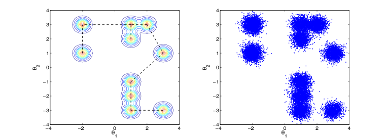
Figure 2: Sampling from a mixture of 10 Gaussian distributions with dimension $D=100$ using WHMC with a vector field ${\boldsymbol{f}}({\boldsymbol{\theta}},{\boldsymbol{v}})$ to enforce moving between modes in higher dimensions.

After adding the vector field, we modify the Hamiltonian equation governing the evolution of ${\boldsymbol{\theta}}$ as follows:

$$\dot{\boldsymbol{\theta}}={\boldsymbol{v}}+{\boldsymbol{f}}({\boldsymbol{\theta}},{\boldsymbol{v}})$$ (3.6)

We also need to adjust the Metropolis acceptance probability accordingly since the transformation is not volume preserving. (More details are provided in the supplementary file.) Figure 2 illustrates this approach based on sampling from a mixture of 10 Gaussian distributions with dimension $D=100$.

To address the second issue, we allow the wormholes to pass through an extra auxiliary dimension to avoid their interference with the existing HMC dynamics in the given parameter space. In particular we introduce an auxiliary variable $\theta_{D+1}\sim\mathcal{N}(0,1)$ corresponding to an auxiliary dimension. We use $\tilde{\boldsymbol{\theta}}:=({\boldsymbol{\theta}},\theta_{D+1})$ to denote the position parameters in the resulting $D+1$ dimensional space $\mathcal{M}^{D}\times\mathbb{R}$. $\theta_{D+1}$ can be viewed as random noise independent of $\boldsymbol{\theta}$ and contributes $\frac{1}{2}\theta_{D+1}^{2}$ to the total potential energy. Correspondingly, we augment velocity ${\boldsymbol{v}}$ with one extra dimension, denoted as $\tilde{\boldsymbol{v}}:=({\boldsymbol{v}},v_{D+1})$. At the end of the sampling, we project $\tilde{\boldsymbol{\theta}}$ to the original parameter space and discard $\theta_{D+1}$.

We refer to $\mathcal{M}^{D}\times\{-h\}$ as the real world, and call $\mathcal{M}^{D}\times\{+h\}$ the mirror world. Here, $h$ is half of the distance between the two worlds, and it should be in the same scale as the average distance between the modes. For most of the examples discussed here, we set $h=1$. Figure 3 illustrates how the two worlds are connected by networks of wormholes. When the sampler is near a mode $(\hat{\boldsymbol{\theta}}_{1},-h)$ in the real world, we build a wormhole network by connecting it to all the modes in the mirror world. Similarly, we connect the corresponding mode in the mirror world, $(\hat{\boldsymbol{\theta}}_{1},+h)$, to all the modes in the real world. Such construction allows the sampler to jump from one mode in the real world to the same mode in the mirror world and vice versa. This way, the algorithm can effectively sample from the vicinity of a mode, while occasionally jumping from one mode to another.

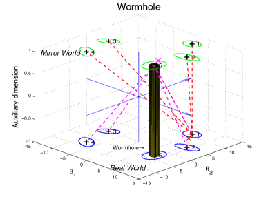
Figure 3: Illustrating a wormhole network connecting the real world to the mirror world ($h=1$). As an example, the cylinder shows a wormhole connecting mode 5 in the real world to its mirror image. The dashed lines show two sets of wormholes. The red lines shows the wormholes when the sampler is close to mode 1 in the real world, and the magenta lines show the wormholes when the sampler is close to mode 5 in the mirror world.

The attached supplementary file provides the details of our algorithm (Algorithm 1), along with the proof of convergence and its implementation in MATLAB.

4 Mode Searching After Regeneration

So far, we assumed that the locations of modes are known. This is of course not a realistic assumption in many situations. In this section, we relax this assumption by extending our method to search for new modes proactively and to update the network of wormholes dynamically. In general, however, allowing such adaptation to take place infinitely often will disturb the stationary distribution of the chain, rendering the process no longer Markov (Gelfand and Dey, 1994; Gilks et al., 1998). To avoid this issue, we use the regeneration method discussed by Nummelin (1984); Mykland et al. (1995); Gilks et al. (1998); Brockwell and Kadane (2005).

Informally, a regenerative process “starts again” probabilistically at a set of times, called regeneration times (Brockwell and Kadane, 2005). At regeneration times, the transition mechanism can be modified based on the entire history of the chain up to that point without disturbing the consistency of MCMC estimators.

4.1 Identifying Regeneration Times

The main idea behind finding regeneration times is to regard the transition kernel $T(\boldsymbol{\theta}_{t+1}|\boldsymbol{\theta}_{t})$ as a mixture of two kernels, $Q$ and $R$ (Nummelin, 1984; Ahn et al., 2013),

$$T(\boldsymbol{\theta}_{t+1}|\boldsymbol{\theta}_{t})=S(\boldsymbol{\theta}_{t})Q(\boldsymbol{\theta}_{t+1})+(1-S(\boldsymbol{\theta}_{t}))R(\boldsymbol{\theta}_{t+1}|\boldsymbol{\theta}_{t})$$

where $Q({\boldsymbol{\theta}}_{t+1})$ is an independence kernel, and the residual kernel $R(\boldsymbol{\theta}_{t+1}|\boldsymbol{\theta}_{t})$ is defined as follows:

$$\!\!R(\boldsymbol{\theta}_{t+1}|\boldsymbol{\theta}_{t})\!\!=\!\!\begin{dcases}\frac{T(\boldsymbol{\theta}_{t+1}|\boldsymbol{\theta}_{t})-S(\boldsymbol{\theta}_{t})Q(\boldsymbol{\theta}_{t+1})}{1-S(\boldsymbol{\theta}_{t})},&\!\!\!\!S(\boldsymbol{\theta}_{t})\in[0,1)\\ 1,&\!\!\!\!S(\boldsymbol{\theta}_{t})=1\end{dcases}$$

$S(\boldsymbol{\theta}_{t})$ is the mixing coefficient between the two kernels such that

$$T(\boldsymbol{\theta}_{t+1}|\boldsymbol{\theta}_{t})\geq S(\boldsymbol{\theta}_{t})Q(\boldsymbol{\theta}_{t+1}),\forall\boldsymbol{\theta}_{t},\boldsymbol{\theta}_{t+1}$$ (4.1)

Now suppose that at iteration $t$, the current state is $\boldsymbol{\theta}_{t}$. To implement this approach, we first generate $\boldsymbol{\theta}_{t+1}$ using the original transition kernel $\boldsymbol{\theta}_{t+1}|\boldsymbol{\theta}_{t}\sim T(\cdot|\boldsymbol{\theta}_{t})$. Then, we sample $B_{t+1}$ from a Bernoulli distribution with probability

$$r(\boldsymbol{\theta}_{t},\boldsymbol{\theta}_{t+1})=\frac{S(\boldsymbol{\theta}_{t})Q(\boldsymbol{\theta}_{t+1})}{T(\boldsymbol{\theta}_{t+1}|\boldsymbol{\theta}_{t})}$$ (4.2)

If $B_{t+1}=1$, a regeneration has occurred, then we discard $\boldsymbol{\theta}_{t+1}$ and sample it from the independence kernel $\boldsymbol{\theta}_{t+1}\sim Q(\cdot)$. At regeneration times, we redefine the dynamics using the past sample path.

Ideally, we would like to evaluate regeneration times in terms of WHMC’s transition kernel. In general, however, this is quite difficult for such Metropolis algorithms. On the other hand, regenerations are easily achieved for the independence sampler (i.e., the proposed state is independent from the current state) as long as the proposal distribution is close to the target distribution (Gilks et al., 1998). Therefore, we can specify a hybrid sampler that consists of the original proposal distribution (here, WHMC) and the independence sampler, and adapt both proposal distributions whenever a regeneration is obtained on an independence-sampler step (Gilks et al., 1998). In our method, we systematically alternate between WHMC and the independence sampler while evaluating regeneration times based on the independence sampler only.

As mentioned above, for this method to be effective, the proposal distribution for the independence sampler should be close to the target distribution. To this end, we follow Ahn et al. (2013) and specify our independence sampler as a mixture of Gaussians located at the previously identified modes. The covariance matrix for each mixture component is set to the inverse observed Fisher information (i.e., Hessian) evaluated at the mode. The relative weight of each mixture component set to $1/k$ at the beginning, where $k$ is the number of previously identified modes through some initial optimization algorithm. The weights are updated at regeneration times to be proportional to the number of times the corresponding mode has been visited. More specifically, $T(\boldsymbol{\theta}_{t+1}|\boldsymbol{\theta}_{t})$, $S(\boldsymbol{\theta}_{t})$ and $Q(\boldsymbol{\theta}_{t+1})$ are defined as follows to satisfy (4.1):

$$T(\boldsymbol{\theta}_{t+1}|\boldsymbol{\theta}_{t}) =q(\boldsymbol{\theta}_{t+1})\min\left\{1,\frac{\pi(\boldsymbol{\theta}_{t+1})/q(\boldsymbol{\theta}_{t+1})}{\pi(\boldsymbol{\theta}_{t})/q(\boldsymbol{\theta}_{t})}\right\}$$ (4.3)

$$S(\boldsymbol{\theta}_{t}) =\min\left\{1,\frac{c}{\pi(\boldsymbol{\theta}_{t})/q(\boldsymbol{\theta}_{t})}\right\}$$ (4.4)

$$Q(\boldsymbol{\theta}_{t+1}) =q(\boldsymbol{\theta}_{t+1})\min\left\{1,\frac{\pi(\boldsymbol{\theta}_{t+1})/q(\boldsymbol{\theta}_{t+1})}{c}\right\}$$ (4.5)

where $q(\cdot)$ is the independence proposal kernel, which specified using a mixture of Gaussians with means fixed at the $k$ known modes prior to regeneration. Algorithm 2 in the supplementary file shows the steps for this method.

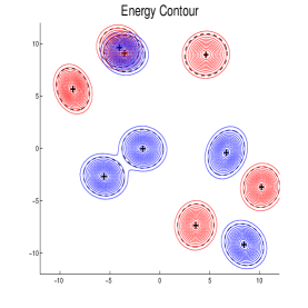
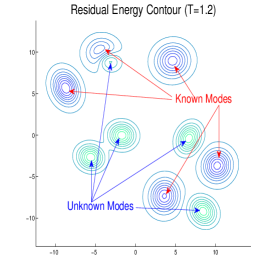
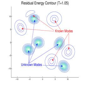
Figure 4: Left panel: True energy function (red: known modes, blue: unknown modes). Middle panel: Residual energy function at $T=1.2$. Right panel: Residual energy function at $T=1.05$.

4.2 Identifying New Modes

When the chain regenerates, we can search for new modes, modify the transition kernel by including newly found modes in the mode library, and update the wormhole network accordingly. This way, starting with a limited number of modes (identified by some preliminary optimization method), WHMC could discover unknown modes on the fly without affecting the stationarity of the chain.

To search for new modes after regeneration, we could simply apply an optimization algorithm to the original target density function $\pi(\boldsymbol{\theta})$ with some random starting points. This, however, could lead to frequently rediscovering the known modes. To avoid this issue, we propose to remove/down-weight the known modes using the history of the chain up to the regeneration time and run an optimization algorithm on the resulting residual density, or equivalently, on the corresponding residual energy (i.e., minus log of density). To this end, we fit a mixture of Gaussians with the best knowledge of modes (locations, Hessians and relative weights) prior to the regeneration. The residual density function could be simply defined as $\pi_{\bf r}(\boldsymbol{\theta})=\pi(\boldsymbol{\theta})-q(\boldsymbol{\theta})$ with the corresponding residual potential energy as follows,

$$U_{\bf r}(\boldsymbol{\theta})=\log(\pi_{\bf r}(\boldsymbol{\theta})+c)=-\log(\pi(\boldsymbol{\theta})-q(\boldsymbol{\theta})+c)$$

where the constant $c>0$ is used to make the term inside the log function positive. To avoid completely flat regions (e.g., when a Gaussian distribution provides a good approximation around the mode), which could cause gradient-based optimization methods to fail, we could use the following tempered residual potential energy instead:

$$U_{\bf r}(\boldsymbol{\theta},T)=-\log\left(\pi(\boldsymbol{\theta})-\exp\left(\frac{1}{T}\log q(\boldsymbol{\theta})\right)+c\right)$$

where $T$ is the temperature. Figure 4 illustrates this concept.

When the optimizer finds new modes, they are added to the existing mode library, and the wormhole network is updated accordingly.

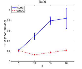
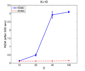
Figure 5: Comparing WHMC to RDMC using $K$ mixtures of $D$-dimensional Gaussians. Left panel: REM (along with 95% confidence interval based on 10 MCMC chains) for varying number of mixture components, $K=5,10,15,20$, with fixed dimension, $D=20$. Right panel: REM (along with 95% confidence interval based on 10 MCMC chains) for varying number of dimensions, $D=10,20,40,100$, with fixed number of mixture components, $K=10$.

5 Empirical Results

In this section, we evaluate the performance of our method, henceforth called Wormhole Hamiltonian Monte Carlo (WHMC), using three examples. The first example involves sampling from mixtures of Gaussian distributions with varying number of modes and dimensions. In this example, which is also discussed by Ahn et al. (2013), the locations of modes are assumed to be known. The second example, which was originally proposed by Ihler et al. (2005), involves inference regarding the locations of sensors in a network. For our third example, we also use mixtures of Gaussian distributions, but this time we assume that the locations of modes are unknown.

We evaluate our method’s performance by comparing it to Regeneration Darting Monte Carlo (RDMC) (Ahn et al., 2013), which is one of the most recent algorithms designed for sampling from multimodal distributions based on the Darting Monte Carlo (DMC) (Sminchisescu and Welling, 2011) approach. DMC defines high density regions around the modes. When the sampler enters these regions, a jump between the regions will be attempted. RDMC enriches the DMC method by using the regeneration approach (Mykland et al., 1995; Gilks et al., 1998).

We compare the two methods (i.e., WHMC and RDMC) in terms of Relative Error of Mean (REM) (Ahn et al., 2013), which summarizes the errors in approximating the expectation of variables across all dimensions, and its value at time $t$ is $\mathrm{REM}(t)=\|\overline{\theta(t)}-\theta^{*}\|_{1}/\|\theta^{*}\|_{1}$. Here, $\overline{\theta(t)}$ is the mean of MCMC samples at time $t$ and $\theta^{*}$ is the true mean. Because RDMC uses standard HMC algorithm with a flat metric, we also use the baseline metric ${\boldsymbol{G}}_{0}\equiv{\boldsymbol{I}}$ to make the two algorithms comparable. Our approach, however, can be easily extended to other metrics such as Fisher information.

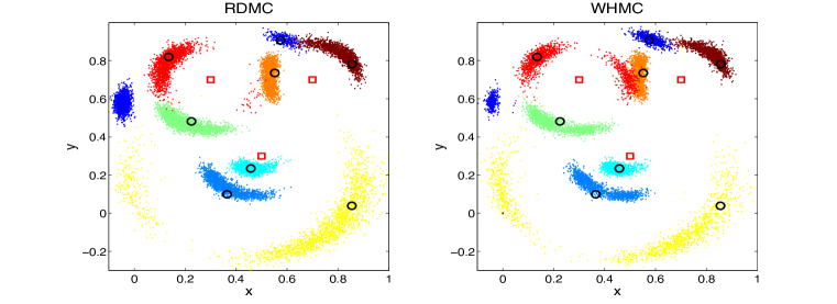
Figure 6: Posterior samples for sensor locations using RDMC (left panel) and WHMC (right panel).

5.1 Mixture of Gaussians with Known Modes

First, we evaluate the performance of our method based on sampling from $K$ mixtures of $D$-dimensional Gaussian distributions with known modes. (We relax this assumption later.) The means of these distributions are randomly generated from $D$-dimensional uniform distributions such that the average pairwise distances remains around 20. The corresponding covariance matrices are constructed in a way that mixture components have different density functions. Simulating samples from the resulting $D$ dimensional mixture of $K$ Gaussians is challenging because the modes are far apart and the high density regions have different shapes.

The left panel of Figure 5 compares the two methods for varying number of mixture components, $K=5,10,15,20$, with fixed dimension ($D=20$). The right panel shows the results for varying number of dimensions, $D=10,20,40,100$, with fixed number of mixture components ($K=10$). For both scenarios, we stop the two algorithms after 500 seconds and compare their REM. As we can see, WHMC has substantially lower REM compared to RDMC, especially when the number of modes and dimensions increase.

5.2 Sensor Network Localization

For our second example, we use a problem previously discussed by Ihler et al. (2005) and Ahn et al. (2013). We assume that $N$ sensors are scattered in a planar region with $2d$ locations denoted as $\{x_{i}\}_{i=1}^{N}$. The distance $Y_{ij}$ between a pair of sensors $(x_{i},x_{j})$ is observed with probability $\pi(x_{i},x_{j})=\exp(-\|x_{i}-x_{j}\|^{2}/(2R^{2}))$. If the distance is in fact observed ($Y_{ij}>0$), then $Y_{ij}$ follows a Gaussian distribution $\mathcal{N}(\|x_{i}-x_{j}\|,\sigma^{2})$ with small $\sigma$; otherwise $Y_{ij}=0$. That is,

$$Z_{ij}=I(Y_{ij}>0)|x \sim\mathrm{Binom}(1,\pi(x_{i},x_{j}))$$

$$Y_{ij}|Z_{ij}=1,x \sim\mathcal{N}(\|x_{i}-x_{j}\|,\sigma^{2})$$

where $Z_{ij}$ is a binary indicator set to 1 if the distance between $x_{i}$ and $x_{j}$ is observed.

Given a set of observations $Y_{ij}$ and prior distribution of $x$, which is assumed to be uniform in this example, it is of interest to infer the posterior distribution of all the sensor locations. Following Ahn et al. (2013), we set $N=8,R=0.3,\sigma=0.02$, and add three additional base sensors with known locations to avoid ambiguities of translation, rotation, and negation (mirror symmetry). The location of the 8 sensors form a multimodal distribution with dimension $D=16$.

Figure 6 shows the posterior samples based on the two methods. As we can see, RDMC very rarely visits one of the modes (shown in red in the top middle part); whereas, WHMC generates enough samples from this mode to make it discernible. As a result, WHMC converges to a substantially lower REM ($0.02$) compared to RDMC ($0.13$) after 500 seconds.

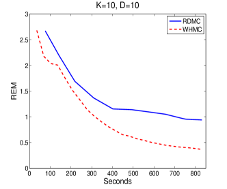
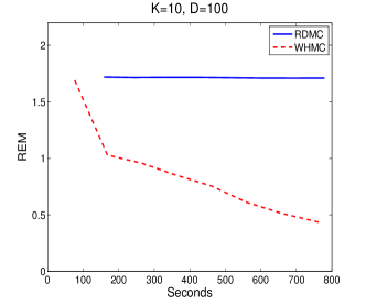
Figure 7: Comparing WHMC to RDMC in terms of REM using $K=10$ mixtures of $D$-dimensional Gaussians with $D=20$ (left panel) and $D=100$ (right panel).

5.3 Mixture of Gaussians with Unknown Modes

We now evaluate our method’s performance in terms of searching for new modes and updating the network of wormholes. For this example, we simulate a mixture of 10 $D$-dimensional Gaussian distributions, with $D=10,100$, and compare our method to RDMC. While RDMC runs four parallel HMC chains initially to discover a subset of modes and to fit a truncated Gaussian distribution around each identified mode, we run four parallel optimizers (different starting points) using the BFGS method. At regeneration times, each chain of RDMC uses the Dirichlet process mixture model to fit a new truncated Gaussian around modes and possibly identify new modes. We on the other hand run the BGFS algorithm based on the residual energy function (with $T=1.05$) to discover new modes for each chain. Figure 7 shows WHMC reduces REM much faster than RDMC for both $D=10$ and $D=100$. Here, the recorded time (horizontal axis) accounts for the computational overhead for adapting the transition kernels. For $D=10$, our method has a substantially lower REM compared to RDMC. For $D=100$, while our method identifies new modes over time and reduces REM substantially, RDMC fails to identify new modes so as a result its REM remains high over time.

6 Conclusions and Discussion

We have proposed a new algorithm for sampling from multimodal distributions. Using empirical results, we have shown that our method performs well in high dimensions.

Our method involves several parameters that require tuning. However, these parameters can be adjusted at regeneration times without affecting the stationary distribution.

Although we used a flat base metric (i.e., $\boldsymbol{I}$) in the examples discussed in this paper, our method can be easily extended by specifying a more informative base metric (e.g., Fisher information) that adapts to local geometry.

Appendix

In this supplementary document, we provide details of our proposed Wormhole Hamiltonian Monte Carlo (WHMC) algorithm and prove its convergence to the stationary distribution. For simplicity, we assume that ${\bf G}(\boldsymbol{\theta})\equiv{\bf I}$. Our results can be extended to more general Riemannian metrics.

In what follows, we first prove the convergence of our method when an external vector field is added to the dynamics. Next, we prove the convergence for our final algorithm, where besides an external vector field, we include an auxiliary dimension along which the network of wormholes are constructed. Finally, we provide our algorithm to identify regeneration times.

Appendix A Adjustment of Metropolis acceptance probability in WHMC with vector field

As mentioned in the paper, in high dimensional problems with isolated modes, the effect of wormhole metric could diminish fast as the sampler leaves one mode towards another mode. To avoid this issue, we have extended our method by including a vector field, ${\bf f}({\boldsymbol{\theta}},{\bf v})$, which depends on a vicinity function illustrated in Figure 8. The resulting dynamics facilitates movements between modes,

$$\dot{\boldsymbol{\theta}} = {\bf v}+{\bf f}({\boldsymbol{\theta}},{\bf v})$$ (A.1)

$$\dot{\bf v} = -\nabla_{\boldsymbol{\theta}}U({\boldsymbol{\theta}})$$

We solve (A.1) using the generalized leapfrog integrator (Leimkuhler and Reich, 2004; Girolami and Calderhead, 2011):

$${\bf v}^{(\ell+1/2)} ={\bf v}^{(\ell)}-\frac{\varepsilon}{2}\nabla_{\boldsymbol{\theta}}U({\boldsymbol{\theta}}^{(\ell)})$$ (A.2)

$${\boldsymbol{\theta}}^{(\ell+1)} ={\boldsymbol{\theta}}^{(\ell)}+\varepsilon[{\bf v}^{(\ell+1/2)}+({\bf f}({\boldsymbol{\theta}}^{(\ell)},{\bf v}^{(\ell+1/2)})+{\bf f}({\boldsymbol{\theta}}^{(\ell+1)},{\bf v}^{(\ell+1/2)}))/2]$$ (A.3)

$${\bf v}^{(\ell+1)} ={\bf v}^{(\ell+1/2)}-\frac{\varepsilon}{2}\nabla_{\boldsymbol{\theta}}U({\boldsymbol{\theta}}^{(\ell+1)})$$ (A.4)

where $\ell$ is the index for leapfrog steps, and ${\bf v}^{(\ell+1/2)}$ denotes the current value of ${\bf v}$ after half a step of leapfrog. The implicit equation (A.3) can be solved by the fixed point iteration.

The integrator (A.2)-(A.4) is time reversible and numerically stable; however, it is not volume preserving. To fix this issue, we can adjust the Metropolis acceptance probability with the Jacobian determinant of the mapping $\hat{T}$ given by (A.2)-(A.4) in order to satisfy the detailed balance condition. Denote ${\bf z}=({\boldsymbol{\theta}},{\bf v})$. Given the corresponding Hamiltonian function, $H({\bf z})$, we define $\mathbb{P}(d{\bf z})=\exp(-H({\bf z}))d{\bf z}$ and prove the following proposition (See Green, 1995).

Proposition 1 (Detailed Balance Condition with determinant adjustment).

Let ${\bf z}^{\prime}=\hat{T}_{L}({\bf z})$ be the proposal according to some time reversible integrator $\hat{T}_{L}$ for dynamics (A.1). Then the detailed balance condition holds given the following adjusted acceptance probability:

$$\tilde{\alpha}({\bf z},{\bf z^{\prime}})=\min\left\{1,\frac{\exp(-H({\bf z^{\prime}}))}{\exp(-H({\bf z}))}|\det d\hat{T}_{L}|\right\}$$ (A.5)

Proof.

To prove detailed balance, we need to show

$$\tilde{\alpha}({\bf z},{\bf z^{\prime}})\mathbb{P}(d{\bf z})=\tilde{\alpha}({\bf z^{\prime}},{\bf z})\mathbb{P}(d{\bf z^{\prime}})$$ (A.6)

The following steps show that this condition holds:

$$\begin{split}\tilde{\alpha}({\bf z},{\bf z^{\prime}})\mathbb{P}(d{\bf z})&=\min\left\{1,\frac{\exp(-H({\bf z^{\prime}}))}{\exp(-H({\bf z}))}\left|\frac{d{\bf z^{\prime}}}{d{\bf z}}\right|\right\}\exp(-H({\bf z}))d{\bf z}\\ &\overset{{\bf z}=\hat{T}_{L}^{-1}({\bf z^{\prime}})}{=}\min\left\{\exp(-H({\bf z})),\exp(-H({\bf z^{\prime}}))\left|\frac{d{\bf z^{\prime}}}{d{\bf z}}\right|\right\}\left|\frac{d{\bf z}}{d{\bf z^{\prime}}}\right|d{\bf z^{\prime}}\\ &=\min\left\{1,\frac{\exp(-H({\bf z}))}{\exp(-H({\bf z^{\prime}}))}\left|\frac{d{\bf z}}{d{\bf z^{\prime}}}\right|\right\}\exp(-H({\bf z^{\prime}}))d{\bf z^{\prime}}=\tilde{\alpha}({\bf z^{\prime}},{\bf z})\mathbb{P}(d{\bf z^{\prime}})\end{split}$$

∎

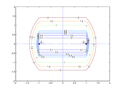
Figure 8: Contour plot of the vicinity function $V(\boldsymbol{\theta})$ in Equation (6) of our paper.

We implement (A.2)-(A.4) for $L$ steps to generate a proposal ${\bf z}^{(L+1)}$ and accept it with the following adjusted probability:

$$\alpha_{VF}({\bf z}^{(1)},{\bf z}^{(L+1)})=\min\{1,\exp(-H({\bf z}^{(L+1)})+H({\bf z}^{(1)}))|\det{\bf J}_{VF}|\}$$

where the Jacobian determinant, $\det{\bf J}_{VF}=\prod_{n=1}^{L}\left|\dfrac{d{\bf z}^{(\ell+1)}}{d{\bf z}^{(\ell)}}\right|=\prod_{n=1}^{L}\left|\dfrac{\partial({\boldsymbol{\theta}}^{(\ell+1)},{\bf v}^{(\ell+1)})}{\partial({\boldsymbol{\theta}}^{(\ell)},{\bf v}^{(\ell)})}\right|$, can be calculated through the following wedge product:

$$d{\boldsymbol{\theta}}^{(\ell+1)}\wedge d{\bf v}^{(\ell+1)}=[{\bf I}-\frac{\varepsilon}{2}\nabla_{{\boldsymbol{\theta}}^{\mathsf{T}}}{\bf f}({\boldsymbol{\theta}}^{(\ell+1)},{\bf v}^{(\ell+1/2)})]^{-1}[{\bf I}+\frac{\varepsilon}{2}\nabla_{{\boldsymbol{\theta}}^{\mathsf{T}}}{\bf f}({\boldsymbol{\theta}}^{(\ell)},{\bf v}^{(\ell+1/2)})]\;d{\boldsymbol{\theta}}^{(\ell)}\wedge d{\bf v}^{(\ell)}$$

with $\nabla_{{\boldsymbol{\theta}}^{\mathsf{T}}}{\bf f}({\boldsymbol{\theta}},{\bf v})={\bf v}^{*}_{W}({\bf v}^{*}_{W})^{\mathsf{T}}{\bf v}\nabla\mathfrak{m}({\boldsymbol{\theta}})^{\mathsf{T}}$ (See Lan et al., 2012, for more details.)

Appendix B WHMC in the augmented $D+1$ dimensional space

Suppose that the current position, $\tilde{\boldsymbol{\theta}}$, of the sampler is near a mode denoted as $\tilde{\boldsymbol{\theta}}^{*}_{0}$. A network of wormholes connects this mode to all the modes in the opposite world $\tilde{\boldsymbol{\theta}}^{*}_{k},k=1,\cdots K$. Wormholes in the augmented space starting from this mode may still interfere each other since they intersect. To resolve this issue, instead of deterministically weighing wormholes by the vicinity function (6), we use the following random vector field $\tilde{\bf f}(\tilde{\boldsymbol{\theta}},\tilde{\bf v})$:

$$\tilde{\bf f}(\tilde{\boldsymbol{\theta}},\tilde{\bf v})\sim\begin{dcases}(1-\sum_{k}\mathfrak{m}_{k}(\tilde{\boldsymbol{\theta}}))\delta_{\tilde{\bf v}}(\cdot)+\sum_{k}\mathfrak{m}_{k}(\tilde{\boldsymbol{\theta}})\delta_{2(\tilde{\boldsymbol{\theta}}^{*}_{k}-\tilde{\boldsymbol{\theta}})/e}(\cdot),&\;\textrm{if}\,\sum_{k}\mathfrak{m}_{k}(\tilde{\boldsymbol{\theta}})<1\\ \frac{\sum_{k}\mathfrak{m}_{k}(\tilde{\boldsymbol{\theta}})\delta_{2(\tilde{\boldsymbol{\theta}}^{*}_{k}-\tilde{\boldsymbol{\theta}})/e}(\cdot)}{\sum_{k}\mathfrak{m}_{k}(\tilde{\boldsymbol{\theta}})},&\;\textrm{if}\,\sum_{k}\mathfrak{m}_{k}(\tilde{\boldsymbol{\theta}})\geq 1\end{dcases}$$

where $e$ is the stepsize, $\delta$ is the Kronecker delta function, and $\mathfrak{m}_{k}(\tilde{\boldsymbol{\theta}})=\exp\{-V_{k}(\tilde{\boldsymbol{\theta}})/(DF)\}$. Here, the vicinity function $V_{k}(\tilde{\boldsymbol{\theta}})$ along the $k$-th wormhole is defined similarly to Equation (6),

$$V_{k}(\tilde{\boldsymbol{\theta}})=\langle\tilde{\boldsymbol{\theta}}-\tilde{\boldsymbol{\theta}}^{*}_{0},\tilde{\boldsymbol{\theta}}-\tilde{\boldsymbol{\theta}}^{*}_{k}\rangle+|\langle\tilde{\boldsymbol{\theta}}-\tilde{\boldsymbol{\theta}}^{*}_{0},\tilde{\bf v}^{*}_{W_{k}}\rangle||\langle\tilde{\boldsymbol{\theta}}-\tilde{\boldsymbol{\theta}}^{*}_{k},\tilde{\bf v}^{*}_{W_{k}}\rangle|$$

where $\tilde{\bf v}^{*}_{W_{k}}=(\tilde{\boldsymbol{\theta}}^{*}_{k}-\tilde{\boldsymbol{\theta}}^{*}_{0})/\|\tilde{\boldsymbol{\theta}}^{*}_{k}-\tilde{\boldsymbol{\theta}}^{*}_{0}\|$.

For each update, $\tilde{\bf f}(\tilde{\boldsymbol{\theta}},\tilde{\bf v})$ is either set to $\tilde{\bf v}$ or $2(\tilde{\boldsymbol{\theta}}^{*}_{k}-\tilde{\boldsymbol{\theta}})/e$ according to the position dependent probabilities defined in terms of $\mathfrak{m}_{k}(\tilde{\boldsymbol{\theta}})$. Therefore, we write the Hamiltonian dynamics in the extended space as follows:

$$\dot{\tilde{\boldsymbol{\theta}}} = \tilde{\bf f}(\tilde{\boldsymbol{\theta}},\tilde{\bf v})$$ (B.1)

$$\dot{\tilde{\bf v}} = -\nabla_{\tilde{\boldsymbol{\theta}}}U(\tilde{\boldsymbol{\theta}})$$

We use (A.2)-(A.4) to numerically solve (B.1), but replace (A.3) with the following equation:

$$\tilde{\boldsymbol{\theta}}^{(\ell+1)}=\tilde{\boldsymbol{\theta}}^{(\ell)}+e/2[\tilde{\bf f}(\tilde{\boldsymbol{\theta}}^{(\ell+1)},\tilde{\bf v}^{(\ell+1/2)})+\tilde{\bf f}(\tilde{\boldsymbol{\theta}}^{(\ell)},\tilde{\bf v}^{(\ell+1/2)})]$$ (B.2)

Note that this is an implicit equation, which can be solved using the fixed point iteration approach (Leimkuhler and Reich, 2004; Girolami and Calderhead, 2011).

According to the above dynamic, at each leapfrog step, $\ell$, the sampler either stays at the vicinity of $\tilde{\boldsymbol{\theta}}^{*}_{0}$ or proposes a move towards a mode $\tilde{\boldsymbol{\theta}}^{*}_{k}$ in the opposite world depending on the values of $\boldsymbol{\tilde{f}}(\tilde{\boldsymbol{\theta}}^{(\ell)}\tilde{\bf v}^{(\ell+1/2)})$ and $\tilde{\bf f}(\tilde{\boldsymbol{\theta}}^{(\ell+1)},\tilde{\bf v}^{(\ell+1/2)})$. For example, if $\tilde{\bf f}(\tilde{\boldsymbol{\theta}}^{(\ell)},\tilde{\bf v}^{(\ell+1/2)})=2(\tilde{\boldsymbol{\theta}}^{*}_{k}-\tilde{\boldsymbol{\theta}}^{(\ell)})/e$, and $\tilde{\bf f}(\tilde{\boldsymbol{\theta}}^{(\ell+1)},\tilde{\bf v}^{(\ell+1/2)})=\tilde{\bf v}^{(\ell+1/2)}$, then equation (B.2) becomes

$$\tilde{\boldsymbol{\theta}}^{(\ell+1)}=\tilde{\boldsymbol{\theta}}^{*}_{k}+\frac{e}{2}\tilde{\bf v}^{(\ell+1/2)}$$

which indicates that a move to the $k$-th mode in the opposite wold has in fact occurred. Note that the movement $\tilde{\boldsymbol{\theta}}^{(\ell)}\to\tilde{\boldsymbol{\theta}}^{(\ell+1)}$ in this case is discontinuous since

$$\lim_{e\to 0}\|\tilde{\boldsymbol{\theta}}^{(\ell+1)}-\tilde{\boldsymbol{\theta}}^{(\ell)}\|\geq 2h>0$$

Therefore, in such cases, there will be an energy gap, $\Delta E:=H(\tilde{\boldsymbol{\theta}}^{(\ell+1)},\tilde{\bf v}^{(\ell+1)})-H(\tilde{\boldsymbol{\theta}}^{(\ell)},\tilde{\bf v}^{(\ell)})$, between the two states. We need to adjust the Metropolis acceptance probability to account for the resulting energy gap. Further, we limit the maximum number of jumps within each iteration of MCMC (i.e., over $L$ leapfrog steps) to 1 so the sampler can explore the vicinity of the new mode before making another jump. Algorithm 1 provides the details of this approach.

We note that according to the definition of $\tilde{\bf f}(\tilde{\boldsymbol{\theta}},\tilde{\bf v})$ and equation (B.2), the jump occurs randomly. We use $\ell^{\prime}$ to denote the step at which the sampler jumps. That is, $\ell^{\prime}$ randomly takes a value in $\{0,1,\cdots,L\}$ depending on $\tilde{\bf f}$. When there is no jump along the trajectory, we set $\Delta E=0$, $\ell^{\prime}=0$, and the algorithm reduces to standard HMC. In the following, we first prove the detailed balance condition when a jump happens, and then use it to prove the convergence of the algorithm to the stationary distribution.

When a mode jumping occurs at some fixed step $\ell^{\prime}$, we can divide the $L$ leapfrog steps into three parts: $\ell^{\prime}-1$ steps continuous movement according to standard HMC, 1 step discontinuous jump, and $L-\ell^{\prime}$ steps according to standard HMC in the opposite world. Note that the Metropolis acceptance probability in standard HMC can be written as

$$\alpha(\tilde{\bf z}^{(L+1)},\tilde{\bf z}^{(1)})=\min\{1,\exp(-H(\tilde{\bf z}^{(L+1)})+H(\tilde{\bf z}^{(1)}))\}=\min\left\{1,\exp\left(-\sum_{\ell=1}^{L}(H(\tilde{\bf z}^{(\ell+1)})-H(\tilde{\bf z}^{(\ell)}))\right)\right\}$$

Each summand $H(\tilde{\bf z}^{(\ell+1)})-H(\tilde{\bf z}^{(\ell)})$ is small ($\mathcal{O}(\varepsilon^{3})$) except for the $\ell^{\prime}$-th one, where there is an energy gap, $\Delta E$. Given that the jump happens at the $\ell^{\prime}$-th step, we should remove the $\ell^{\prime}$-th summand from the acceptance probability:

$$\alpha_{RVF}(\tilde{\bf z}^{(1)},\tilde{\bf z}^{(L+1)}) =\min\left\{1,\exp\left(-\sum_{\ell\neq\ell^{\prime}}(H(\tilde{\bf z}^{(\ell+1)})-H(\tilde{\bf z}^{(\ell)}))\right)\right\}$$

$$=\min\left\{1,\frac{\exp(-H(\tilde{\bf z}^{(L+1)}))}{\exp(-H(\tilde{\bf z}^{(\ell^{\prime}+1)}))}\frac{\exp(-H(\tilde{\bf z}^{(\ell^{\prime})}))}{\exp(-H(\tilde{\bf z}^{(1)}))}\right\}$$ (B.3)

$$=\min\{1,\exp(-H(\tilde{\bf z}^{(L+1)})+H(\tilde{\bf z}^{(1)})+\Delta E)\}$$

That is, we only count the acceptance probability for the first $\ell^{\prime}-1$ and the last $L-\ell^{\prime}$ steps of continuous movement in standard HMC; at $\ell^{\prime}+1$ step, we “reset” the energy level by accounting for the energy gap $\Delta E$. Therefore, the following proposition is true.

Proposition 2 (Detailed Balance Condition with energy adjustment).

When a discontinuous jump happens in WHMC, we have the following detailed balance condition with the adjusted acceptance probability (B.3).

$$\alpha_{RVF}(\tilde{\bf z}^{(1)},\tilde{\bf z}^{(L+1)})\mathbb{P}(d\tilde{\bf z}^{(1)})\mathbb{P}(d\tilde{\bf z}^{(\ell^{\prime}+1)})=\alpha_{RVF}(\tilde{\bf z}^{(L+1)},\tilde{\bf z}^{(1)})\mathbb{P}(d\tilde{\bf z}^{(L+1)})\mathbb{P}(d\tilde{\bf z}^{(\ell^{\prime})})$$ (B.4)

Next, we use $\hat{T}_{\ell}:\tilde{\bf z}^{(\ell)}\mapsto\tilde{\bf z}^{(\ell+1)}$ to denote an integrator consisting of (A.2)(B.2)(A.4). Note that $\hat{T}_{\ell}$ depends on $\tilde{\bf f}$. Denote $\hat{T}_{1:\ell}:=\hat{T}_{\ell}\circ\cdots\circ\hat{T}_{1}$. Following Liu (2001), we can prove the following stationarity theorem.

Theorem 1 (Stationarity of WHMC).

The samples given by WHMC (algorithm 1) have the target distribution $\pi(\cdot)$ as its stationarity distribution.

Proof.

Let $\tilde{\bf z}^{*}=\hat{T}_{1:L}(\tilde{\bf z})$. Suppose $\tilde{\boldsymbol{\theta}}^{*}\sim f(\tilde{\boldsymbol{\theta}}^{*})$. We want to prove that $f(\cdot)=\pi(\cdot)$ through $\textrm{E}_{f}[h(\tilde{\boldsymbol{\theta}}^{*})]=\textrm{E}_{\pi}[h(\tilde{\boldsymbol{\theta}}^{*})]$ for any square integrable function $h(\tilde{\boldsymbol{\theta}}^{*})$.

Note that $\tilde{\boldsymbol{\theta}}^{*}$ is either an accepted proposal or the current state after a rejection. Therefore,

$$\begin{split}&\textrm{E}_{f}[h(\tilde{\boldsymbol{\theta}}^{*})]\\ =&\iiint h(\tilde{\boldsymbol{\theta}}^{*})[\alpha(\hat{T}_{1:L}^{-1}(\tilde{\bf z}^{*}),\tilde{\bf z}^{*})\mathbb{P}(d\hat{T}_{1:L}^{-1}(\tilde{\bf z}^{*}))\mathbb{P}(d\hat{T}_{1+\ell^{\prime}:L}^{-1}(\tilde{\bf z}^{*}))+(1-\alpha(\tilde{\bf z}^{*},\hat{T}_{1:L}(\tilde{\bf z}^{*})))\mathbb{P}(d\tilde{\bf z}^{*})\mathbb{P}(d\hat{T}_{1:\ell^{\prime}}(\tilde{\bf z}^{*}))]d\ell^{\prime}\\ =&\int h(\tilde{\boldsymbol{\theta}}^{*})\mathbb{P}(d\tilde{\bf z}^{*})+\\ &\iiint h(\tilde{\boldsymbol{\theta}}^{*})[\alpha(\hat{T}_{1:L}^{-1}(\tilde{\bf z}^{*}),\tilde{\bf z}^{*})\mathbb{P}(d\hat{T}_{1:L}^{-1}(\tilde{\bf z}^{*}))\mathbb{P}(d\hat{T}_{1+\ell^{\prime}:L}^{-1}(\tilde{\bf z}^{*}))-\alpha(\tilde{\bf z}^{*},\hat{T}_{1:L}(\tilde{\bf z}^{*}))\mathbb{P}(d\tilde{\bf z}^{*})\mathbb{P}(d\hat{T}_{1:\ell^{\prime}}(\tilde{\bf z}^{*}))]d\ell^{\prime}\end{split}$$

Therefore, it suffices to prove that

$$\iiint h(\tilde{\boldsymbol{\theta}}^{*})\alpha(\hat{T}_{1:L}^{-1}(\tilde{\bf z}^{*}),\tilde{\bf z}^{*})\mathbb{P}(d\hat{T}_{1:L}^{-1}(\tilde{\bf z}^{*}))\mathbb{P}(d\hat{T}_{1+\ell^{\prime}:L}^{-1}(\tilde{\bf z}^{*}))d\ell^{\prime}=\iiint h(\tilde{\boldsymbol{\theta}}^{*})\alpha(\tilde{\bf z}^{*},\hat{T}_{1:L}(\tilde{\bf z}^{*}))\mathbb{P}(d\tilde{\bf z}^{*})\mathbb{P}(d\hat{T}_{1:\ell^{\prime}}(\tilde{\bf z}^{*}))d\ell^{\prime}$$ (B.5)

Based on its construction, $\hat{T}_{\ell}$ is time reversible for all $\ell$. Denote the involution $\nu:(\tilde{\boldsymbol{\theta}},\tilde{\bf v})\mapsto(\tilde{\boldsymbol{\theta}},-\tilde{\bf v})$. We have $\hat{T}^{-1}_{\ell}(\tilde{\bf z}^{*})=\nu\hat{T}_{\ell}\nu(\tilde{\bf z}^{*})$. Further, because $E$ is quadratic in $\tilde{\bf v}$, we have $H(\nu(\tilde{\bf z}))=H(\tilde{\bf z})$. Therefore $\alpha(\nu(\tilde{\bf z}),\tilde{\bf z}^{\prime})=\alpha(\tilde{\bf z},\nu(\tilde{\bf z}^{\prime}))$. Then the left hand side of (B.5) becomes

$$\begin{split}\textrm{LHS}&=\iiint h(\tilde{\boldsymbol{\theta}}^{*})\alpha(\nu\hat{T}_{1:L}\nu(\tilde{\bf z}^{*}),\tilde{\bf z}^{*})\mathbb{P}(d\nu\hat{T}_{1:L}\nu(\tilde{\bf z}^{*}))\mathbb{P}(d\nu\hat{T}_{1+\ell^{\prime}:L}\nu(\tilde{\bf z}^{*}))d\ell^{\prime}\\ &=\iiint h(\tilde{\boldsymbol{\theta}}^{*})\alpha(\hat{T}_{1:L}\nu(\tilde{\bf z}^{*}),\nu(\tilde{\bf z}^{*}))\mathbb{P}(d\hat{T}_{1:L}\nu(\tilde{\bf z}^{*}))\mathbb{P}(d\hat{T}_{1+\ell^{\prime}:L}\nu(\tilde{\bf z}^{*}))d\ell^{\prime}\\ &\overset{\nu(\tilde{\bf z}^{*})\mapsto\tilde{\bf z}^{*}}{=}\iiint h(\tilde{\boldsymbol{\theta}}^{*})\alpha(\hat{T}_{1:L}(\tilde{\bf z}^{*}),\tilde{\bf z}^{*})\mathbb{P}(d\hat{T}_{1:L}(\tilde{\bf z}^{*}))\mathbb{P}(d\hat{T}_{1+\ell^{\prime}:L}(\tilde{\bf z}^{*}))d\ell^{\prime}\end{split}$$

On the other hand, by the detailed balance condition (B.4), the right hand side of (B.5) becomes

$$\textrm{RHS}=\iiint h(\tilde{\boldsymbol{\theta}}^{*})\alpha(\hat{T}_{1:L}(\tilde{\bf z}^{*}),\tilde{\bf z}^{*})\mathbb{P}(d\hat{T}_{1:L}(\tilde{\bf z}^{*}))\mathbb{P}(d\hat{T}_{1:\ell^{\prime}-1}(\tilde{\bf z}^{*}))d\ell^{\prime}$$

Note that $\mathbb{P}(d\hat{T}_{1+\ell^{\prime}:L}(\tilde{\bf z}^{*}))=\mathbb{P}(d\hat{T}_{1:\ell^{\prime}-1}(\tilde{\bf z}^{*}))$ since both $\hat{T}_{1+\ell^{\prime}:L}$ and $\hat{T}_{1:\ell^{\prime}-1}$ are leapfrog steps of standard HMC (no jump). The difference in the numbers of leapfrog steps (i.e., $L-\ell^{\prime}$ and $\ell^{\prime}-1$) does not affect the stationarity since the number of leapfrog steps can be randomized in HMC (Neal, 2010). Therefore, we have $\textrm{LHS}=\textrm{RHS}$, which proves (B.5). ∎

Algorithm 1 Wormhole Hamilton Monte Carlo (WHMC)

  Prepare the modes ${\boldsymbol{\theta}}^{*}_{k},\;k=1,\cdots K$

  Set $\tilde{\boldsymbol{\theta}}^{(1)}=\textrm{current}\;\tilde{\boldsymbol{\theta}}$

  Sample velocity $\tilde{\bf v}^{(1)}\sim\mathcal{N}(0,{\bf I}_{D+1})$

  Calculate ${\bf E}(\tilde{\boldsymbol{\theta}}^{(1)},\tilde{\bf v}^{(1)})=U(\tilde{\boldsymbol{\theta}}^{(1)})+K(\tilde{\bf v}^{(1)})$

  Set $\Delta\log\det=0$, $\Delta E=0$, $\mathrm{Jumped}=\mathrm{false}$.

  for $n=1$ to $L$ do

     $\tilde{\bf v}^{(\ell+\frac{1}{2})}=\tilde{\bf v}^{(\ell)}-\frac{e}{2}\nabla_{\tilde{\boldsymbol{\theta}}}U(\tilde{\boldsymbol{\theta}}^{(\ell)})$

     if $\mathrm{Jumped}$ then

        $\tilde{\boldsymbol{\theta}}^{(\ell+1)}=\tilde{\boldsymbol{\theta}}^{(\ell)}+e\tilde{\bf v}^{(\ell+\frac{1}{2})}$

     else

        Find the closest mode $\tilde{\boldsymbol{\theta}}^{*}_{0}$ and build a network connecting it to all modes $\tilde{\boldsymbol{\theta}}^{*}_{k},\;k=1,\cdots K$ in the opposite world

        for $m=1$ to $M$ do

           Calculate $\mathfrak{m}_{k}(\hat{\tilde{\boldsymbol{\theta}}}^{(m)}),k=1,\cdots K$

           Sample $u\sim\mathrm{Unif}(0,1)$

           if $u<1-\sum_{k}\mathfrak{m}_{k}(\hat{\tilde{\boldsymbol{\theta}}}^{(m)})$ then

              Set ${\bf f}(\hat{\tilde{\boldsymbol{\theta}}}^{(m)},\tilde{\bf v}^{(\ell+\frac{1}{2})})=\tilde{\bf v}^{(\ell+\frac{1}{2})}$

           else

              Choose one of the $k$ wormholes according to probability $\{\mathfrak{m}_{k}/\sum_{k^{\prime}}\mathfrak{m}_{k^{\prime}}\}$ and set ${\bf f}(\hat{\tilde{\boldsymbol{\theta}}}^{(m)},\tilde{\bf v}^{(\ell+\frac{1}{2})})=2(\tilde{\boldsymbol{\theta}}^{*}_{k}-\hat{\tilde{\boldsymbol{\theta}}}^{(m)})/e$

           end if

           $\hat{\tilde{\boldsymbol{\theta}}}^{(m+1)}=\tilde{\boldsymbol{\theta}}^{(\ell)}+\frac{e}{2}[{\bf f}(\hat{\tilde{\boldsymbol{\theta}}}^{(m)},\tilde{\bf v}^{(\ell+\frac{1}{2})})+{\bf f}(\tilde{\boldsymbol{\theta}}^{(\ell)},\tilde{\bf v}^{(\ell+\frac{1}{2})})]$

        end for

        $\tilde{\boldsymbol{\theta}}^{(\ell+1)}=\hat{\tilde{\boldsymbol{\theta}}}^{(M+1)}$

     end if

     $\tilde{\bf v}^{(\ell+1)}=\tilde{\bf v}^{(\ell+\frac{1}{2})}-\frac{e}{2}\nabla_{\tilde{\boldsymbol{\theta}}}U(\tilde{\boldsymbol{\theta}}^{(\ell+1)})$

     If a jump has occurred, set $\mathrm{Jumped}=\mathrm{true}$ and calculate energy gap $\Delta E$.

  end for

  Calculate ${\bf E}(\tilde{\boldsymbol{\theta}}^{(L+1)},\tilde{\bf v}^{(L+1)})=U(\tilde{\boldsymbol{\theta}}^{(L+1)})+K(\tilde{\bf v}^{(L+1)})$

  $p=\exp\{-{\bf E}(\tilde{\boldsymbol{\theta}}^{(L+1)},\tilde{\bf v}^{(L+1)})+{\bf E}(\tilde{\boldsymbol{\theta}}^{(1)},\tilde{\bf v}^{(1)})+\Delta E\}$

  Accept or reject the proposal $(\tilde{\boldsymbol{\theta}}^{(L+1)},\tilde{\bf v}^{(L+1)})$ according to $p$

Algorithm 2 Regeneration in Wormhole Hamiltonian Monte Carlo

  Initially search modes $\hat{\boldsymbol{\theta}}_{1},\cdots,\hat{\boldsymbol{\theta}}_{k}$

  for $n=1$ to $L$ do

     Sample $\tilde{\boldsymbol{\theta}}=(\boldsymbol{\theta},\theta_{D+1})$ as the current state according to WHMC (algorithm 1).

     Fit a mixture of Gaussians $q(\boldsymbol{\theta})$ with known modes, Hessians and relative weights. Propose ${\boldsymbol{\theta}}^{*}\sim q(\cdot)$ and accept it with probability $\alpha=\min\left\{1,\frac{\pi({\boldsymbol{\theta}}^{*})/q({\boldsymbol{\theta}}^{*})}{\pi(\boldsymbol{\theta})/q(\boldsymbol{\theta})}\right\}$.

     if ${\boldsymbol{\theta}}^{*}$ accepted then

        Determine if ${\boldsymbol{\theta}}^{*}$ is a regeneration using (9)-(12) with ${\boldsymbol{\theta}}_{t}=\boldsymbol{\theta}$ and ${\boldsymbol{\theta}}_{t+1}={\boldsymbol{\theta}}^{*}$.

        if Regeneration occurs then

           Search new modes by minimizing $U_{\bf r}(\boldsymbol{\theta},T)$; if new modes are discovered, update the mode library, wormhole network, and $q(\boldsymbol{\theta})$.

           Discard ${\boldsymbol{\theta}}^{*}$, sample ${\boldsymbol{\theta}}^{(\ell+1)}\sim Q(\cdot)$ as in (12) using rejection sampling.

        else

           Set ${\boldsymbol{\theta}}^{(\ell+1)}={\boldsymbol{\theta}}^{*}$.

        end if

     else

        Set ${\boldsymbol{\theta}}^{(\ell+1)}=\tilde{\boldsymbol{\theta}}$.

     end if

  end for

References

- Ahn et al. (2013) S. Ahn, Y. Chen, and M. Welling. Distributed and adaptive darting Monte Carlo through regenerations. In Proceedings of the 16th International Conference on Artificial Intelligence and Statistics (AI Stat), 2013.
- Amari and Nagaoka (2000) S. Amari and H. Nagaoka. Methods of Information Geometry, volume 191 of Translations of Mathematical monographs. Oxford University Press, 2000.
- Braak (2006) C. J. F. Ter Braak. A markov chain monte carlo version of the genetic algorithm differential evolution: easy bayesian computing for real parameter spaces. Statistics and Computing, 16(3):239–249, 2006.
- Brockwell and Kadane (2005) Anthony E. Brockwell and Joseph B. Kadane. Identification of regeneration times in mcmc simulation, with application to adaptive schemes. Journal of Computational and Graphical Statistics, 14:436–458, 2005.
- Celeux et al. (2000) G. Celeux, M. Hurn, and C. P. Robert. Computational and inferential difficulties with mixture posterior distributions. Journal of the American Statistical Association, 95:957–970, 2000.
- Craiu et al. (2009) R. V. Craiu, Jeffrey R., and Chao Y. Learn from thy neighbor: Parallel-chain and regional adaptive mcmc. Journal of the American Statistical Association, 104(488):1454–1466, 2009.
- Duane et al. (1987) S. Duane, A. D. Kennedy, B J. Pendleton, and D. Roweth. Hybrid Monte Carlo. Physics Letters B, 195(2):216 – 222, 1987.
- Gelfand and Dey (1994) A. E. Gelfand and D. K. Dey. Bayesian model choice: Asymptotic and exact calculation. Journal of the Royal Statistical Society. Series B., 56(3):501–514, 1994.
- Gilks et al. (1998) Walter R. Gilks, Gareth O. Roberts, and Sujit K. Sahu. Adaptive markov chain monte carlo through regeneration. Journal of the American Statistical Association, 93(443):pp. 1045–1054, 1998. ISSN 01621459.
- Girolami and Calderhead (2011) M. Girolami and B. Calderhead. Riemann manifold Langevin and Hamiltonian Monte Carlo methods. Journal of the Royal Statistical Society, Series B, (with discussion) 73(2):123–214, 2011.
- Green (1995) Peter J. Green. Reversible jump markov chain monte carlo computation and bayesian model determination. Biometrika, 82:711–732, 1995.
- Hinton et al. (2004) G. E. Hinton, M. Welling, and A. Mnih. Wormholes improve contrastive divergence. In Advances in Neural Information Processing Systems 16, 2004.
- Ihler et al. (2005) A. T. Ihler, J. W. Fisher III, R. L. Moses, and A. S. Willsky. Nonparametric belief propagation for self-localization of sensor networks. IEEE Journal on Selected Areas in Communications, 23(4):809–819, 2005.
- Kirkpatrick et al. (1983) S. Kirkpatrick, C. D. Gelatt, and M. P. Vecchi. Optimization by Simulated Annealing. Science, Number 4598, 13 May 1983, 220(4598):671–680, 1983.
- Kleinberg and Tardos (2005) J. Kleinberg and E. Tardos. Algorithm Design. Addison-Wesley Longman Publishing Co., Inc., Boston, MA, USA, 2005. ISBN 0321295358.
- Lan et al. (2012) S. Lan, V. Stathopoulos, B. Shahbaba, and M. Girolami. Lagrangian Dynamical Monte Carlo. arxiv.org/abs/1211.3759, 2012.
- Laskey and Myers (2003) K. B. Laskey and J. W. Myers. Population Markov Chain Monte Carlo. Machine Learning, 50:175–196, 2003.
- Leimkuhler and Reich (2004) B. Leimkuhler and S. Reich. Simulating Hamiltonian Dynamics. Cambridge University Press, 2004.
- Liu (2001) Jun S. Liu. Monte Carlo Strategies in Scientific Computing, chapter Molecular Dynamics and Hybrid Monte Carlo. Springer-Verlag, 2001.
- Mykland et al. (1995) Per Mykland, Luke Tierney, and Bin Yu. Regeneration in markov chain samplers. Journal of the American Statistical Association, 90(429):pp. 233–241, 1995. ISSN 01621459.
- Neal (1993) R. M. Neal. Probabilistic Inference Using Markov Chain Monte Carlo Methods. Technical Report CRG-TR-93-1, Department of Computer Science, University of Toronto, 1993.
- Neal (2001) R. M. Neal. Annealed importance sampling. Statistics and Computing, 11(2):125–139, 2001.
- Neal (2010) R. M. Neal. MCMC using Hamiltonian dynamics. In S. Brooks, A. Gelman, G. Jones, and X. L. Meng, editors, Handbook of Markov Chain Monte Carlo. Chapman and Hall/CRC, 2010.
- Neal (1996) Radford M. Neal. Bayesian Learning for Neural Networks. Springer-Verlag New York, Inc., Secaucus, NJ, USA, 1996. ISBN 0387947248.
- Nummelin (1984) Esa Nummelin. General Irreducible Markov Chains and Non-Negative Operators, volume 83 of Cambridge Tracts in Mathematics. Cambridge University Press, 1984.
- Rudoy and Wolfe (2006) D. Rudoy and P. J. Wolfe. Monte carlo methods for multi-modal distributions. In Signals, Systems and Computers, 2006. ACSSC ’06. Fortieth Asilomar Conference on, pages 2019–2023, 2006.
- Sminchisescu and Triggs (2002) C. Sminchisescu and B. Triggs. Building roadmaps of local minima of visual models. In In European Conference on Computer Vision, pages 566–582, 2002.
- Sminchisescu and Welling (2011) C. Sminchisescu and M. Welling. Generalized darting monte carlo. Pattern Recognition, 44(10-11), 2011.
- Warnes (2001) G. R. Warnes. The normal kernel coupler: An adaptive Markov Chain Monte Carlo method for efficiently sampling from multi-modal distributions. Technical Report Technical Report No. 395, University of Washington, 2001.
- Welling and Teh (2011) M. Welling and Y. W. Teh. Bayesian learning via stochastic gradient Langevin dynamics. In Proceedings of the International Conference on Machine Learning, 2011.