Decomposition in conic optimization with partially separable structure

Abstract

Decomposition techniques for linear programming are difficult to extend to conic optimization problems with general non-polyhedral convex cones because the conic inequalities introduce an additional nonlinear coupling between the variables. However in many applications the convex cones have a partially separable structure that allows them to be characterized in terms of simpler lower-dimensional cones. The most important example is sparse semidefinite programming with a chordal sparsity pattern. Here partial separability derives from the clique decomposition theorems that characterize positive semidefinite and positive-semidefinite-completable matrices with chordal sparsity patterns. The paper describes a decomposition method that exploits partial separability in conic linear optimization. The method is based on Spingarn’s method for equality constrained convex optimization, combined with a fast interior-point method for evaluating proximal operators.

1 Introduction

We consider conic linear optimization problems (conic LPs)

$$\begin{array}[]{ll}\mbox{minimize}&c^{T}x\\ \mbox{subject to}&Ax=b\\ &x\in\mathcal{C}\end{array}$$ (1)

in which the cone $\mathcal{C}$ is defined in terms of lower-dimensional convex cones $\mathcal{C}_{k}$ as

$$\mathcal{C}=\{x\in{\mbox{\bf R}}^{n}\mid x_{\gamma_{k}}\in\mathcal{C}_{k},\;k=1,\ldots,l\}.$$ (2)

The sets $\gamma_{k}$ are ordered subsets of $\{1,2,\ldots,n\}$ and $x_{\gamma_{k}}$ denotes the subvector of $x$ with entries indexed by $\gamma_{k}$. We refer to the structure in the cone $\mathcal{C}$ as partial separability. The purpose of the paper is to describe a decomposition method that exploits partially separable structure.

In (standard) linear optimization, with $\mathcal{C}={\mbox{\bf R}}^{n}_{+}$, the cone is separable, i.e., a product of one-dimensional cones, and the coupling of variables and constraints is entirely specified by the sparsity pattern of $A$. The term decomposition in linear optimization usually refers to techniques for exploiting angular or dual-angular structure in the coefficient matrix $A$, i.e., a sparsity pattern that is almost block-diagonal, except for a small number of dense rows or columns [Las02, BT97]. The goal of a decomposition algorithm is to solve the problem iteratively, by solving a sequence of separable problems, obtained by removing the complicating variables or constraints. The decoupled subproblems can be solved in parallel or sequentially (for example, to reduce memory usage). Moreover, if the iterative coordinating process is simple enough to be decentralized, the decomposition method can be used as a distributed algorithm. By extension, decomposition methods can also be applied to more general sparsity patterns for which removal of complicating variables and constraints makes the problem substantially easier to solve (even if it does not decompose into independent subproblems).

When the cone $\mathcal{C}$ in (1) is not separable or block-separable (a product of lower-dimensional cones), the formulation of decomposition algorithms is more complicated because the inequalities introduce an additional coupling between the variables. However if the cone is partially separable, as defined in (2), and the overlap between the index sets $\gamma_{k}$ is small, one can still formulate efficient decomposition algorithms. The purpose of this paper is to discuss such a decomposition method. The method is based on Spingarn’s method of partial inverses for convex optimization problems with equality constraints [Spi83, Spi85], combined with an interior-point method applied to sparse conic subproblems. The details of the method are described in sections 2 and 3.

An important example of a partially separable cone are the positive-semidefinite-completable sparse matrices with a chordal sparsity pattern. Matrices in this cone are characterized by the property that all their principal dense submatrices are positive semidefinite [GJSW84, theorem 7]. This fundamental result has been applied in previous methods for sparse semidefinite optimization. It is the basis of the conversion methods used to reformulate sparse semidefinite programs (SDPs) in equivalent forms that are easier to handle by interior-point algorithms [KKMY11, FKMN00] or more suitable for distributed algorithms via the Alternating Direction Method of Multipliers (ADMM) [DZG12]. Partial separability also underlies the saddle-point mirror-prox algorithm for ‘well-structured’ sparse SDPs proposed by Lu, Nemirovski and Monteiro [LNM07]. We discuss the sparse semidefinite optimization application of the decomposition method in detail in sections 4–6.

Notation

If $\alpha$ is a subset of $\{1,2,\ldots,n\}$, then $E_{\alpha}$ will denote the $|\alpha|\times n$-matrix with entries

$$(E_{\alpha})_{ij}=\left\{\begin{array}[]{ll}1&\alpha(i)=j\\ 0&\mbox{otherwise}.\end{array}\right.$$

Here $\alpha(i)$ is the $i$th element of $\alpha$, sorted using the natural ordering. If not explicitly stated the column dimension $n$ of $E_{\alpha}$ will be clear from the context. The result of multiplying an $n$-vector $x$ with $E_{\alpha}$ is the subvector of $x$ of length $|\alpha|$ with elements $(x_{\alpha})_{k}=x_{\alpha(k)}$. The adjoint operation $x=E_{\alpha}^{T}y$ maps an $|\alpha|$-vector $y$ to an $n$-vector $x$ by copying the entries of $y$ to the positions indicated by $\alpha$, i.e., by setting $x_{\alpha(k)}=y_{k}$ and $x_{i}=0$ for $i\not\in\alpha$. Therefore $E_{\alpha}E_{\alpha}^{T}$ is an identity matrix of order $|\alpha|$ and $E_{\alpha}^{T}E_{\alpha}$ is a diagonal $0$-$1$ matrix of order $n$, with $i$th diagonal entry equal to one if and only if $i\in\alpha$. The matrix $P_{\alpha}=E_{\alpha}^{T}E_{\alpha}$ represents projection in ${\mbox{\bf R}}^{n}$ on the sparse $n$-vectors with support $\alpha$.

Similar notation will be used for principal submatrices in a symmetric matrix. If $X\in{\mbox{\bf S}}^{p}$ (the symmetric matrices of order $p$) and $\alpha$ is a subset of $\{1,\ldots,p\}$, then

$$\mathcal{E}_{\alpha}(X)=X_{\alpha\alpha}=E_{\alpha}XE_{\alpha}^{T}\in{\mbox{\bf S}}^{|\alpha|}.$$

This is the submatrix of order $|\alpha|$ with $i,j$ entry $(X_{\alpha\alpha})_{ij}=X_{\alpha(i)\alpha(j)}$. The adjoint operation $\mathcal{E}_{\alpha}^{*}$ copies a matrix $Y\in{\mbox{\bf S}}^{|\alpha|}$ to an otherwise zero symmetric $p\times p$-matrix:

$$\mathcal{E}_{\alpha}^{*}(Y)=E_{\alpha}^{T}YE_{\alpha}.$$

The projection of a matrix $X\in{\mbox{\bf S}}^{p}$ on the matrices that are zero outside of a diagonal $\alpha\times\alpha$ block is denoted

$$\mathcal{P}_{\alpha}(X)=P_{\alpha}XP_{\alpha}=E_{\alpha}^{T}E_{\alpha}XE_{\alpha}^{T}E_{\alpha}.$$

2 Partially separable cones

2.1 Partially separable functions

A function $f:{\mbox{\bf R}}^{n}\rightarrow{\mbox{\bf R}}$ is partially separable if it can be expressed as

$$f(x)=\sum_{k=1}^{l}f_{k}(A_{k}x),$$

where each $A_{k}$ has a nontrivial nullspace, i.e., a rank substantially less than $n$. This concept was introduced by Griewank and Toint in the context of quasi-Newton algorithms [GT82, GT84][NW06, section 7.4]. Here we consider the simplest and most common example of partial separability and assume that $A_{k}=E_{\gamma_{k}}$ for some index set $\gamma_{k}\subset\{1,2,\ldots,n\}$. This means that $f$ can be written as a sum of functions that depend only on subsets of the components of $x$:

$$f(x)=\sum_{k=1}^{l}f_{k}(E_{\gamma_{k}}x)=\sum_{k=1}^{l}f_{k}(x_{\gamma_{k}}).$$ (3)

Partial separability generalizes separability ($l=n$, $\gamma_{k}=\{k\}$) and block-separability (the sets $\gamma_{k}$ form a partition of $\{1,2,\ldots,n\}$).

2.2 Partially separable cones

We call a cone $\mathcal{C}\subset{\mbox{\bf R}}^{n}$ partially separable if it can be expressed as

$$\mathcal{C}=\{x\mid E_{\gamma_{k}}x\in\mathcal{C}_{k},\;k=1,\ldots,l\}$$ (4)

where $\mathcal{C}_{k}$ is a convex cone in ${\mbox{\bf R}}^{|\gamma_{k}|}$. The terminology is motivated by the fact the indicator function $\delta_{\mathcal{C}}$ of $\mathcal{C}$ is a partially separable function:

$$\delta_{\mathcal{C}}(x)=\sum_{k=1}^{p}\delta_{\mathcal{C}_{k}}(E_{\gamma_{k}}x)$$

where $\delta_{\mathcal{C}_{k}}$ is the indicator function of $\mathcal{C}_{k}$. The following assumptions will be made.

• The index sets $\gamma_{k}$ are distinct and maximal, i.e., $\gamma_{i}\not\subseteq\gamma_{j}$ for $i\neq j$, and their union is equal to $\{1,2,\ldots,n\}$.

• The convex cones $\mathcal{C}_{k}$ are proper, i.e., closed, pointed, with nonempty interior. This implies that their dual cones

  $$\mathcal{C}_{k}^{*}=\{v\in{\mbox{\bf R}}^{|\gamma_{k}|}\mid u^{T}v\geq 0\;\forall u\in\mathcal{C}_{k}\}$$

  are proper convex cones and that $\mathcal{C}_{k}=\mathcal{C}_{k}^{**}$ [BV04, page 53].

• There exists a point $\bar{x}$ with $E_{\gamma_{k}}\bar{x}\in\mathop{\bf int}\mathcal{C}_{k}$ for $k=1,\ldots,l$.

These assumptions imply that $\mathcal{C}$ is itself a proper cone. Indeed, $\mathcal{C}$ is clearly convex, with nonempty interior (the point $\bar{x}$ is in the interior). It is closed because it can be expressed as an intersection of closed halfspaces:

$$\mathcal{C}=\{x\in{\mbox{\bf R}}^{n}\mid v_{k}^{T}E_{\gamma_{k}}x\geq 0\;\;\forall v_{k}\in\mathcal{C}_{k}^{*},\;k=1,\ldots,l\}.$$

Finally, $\mathcal{C}$ is pointed because $x\in\mathcal{C}$, $-x\in\mathcal{C}$ implies $E_{\gamma_{k}}x\in\mathcal{C}_{k}$ and $-E_{\gamma_{k}}x\in\mathcal{C}_{k}$ for all $k$. Since the cones $\mathcal{C}_{k}$ are pointed, this means $E_{\gamma_{k}}x=0$ for $k=1,\ldots,l$. Since the index sets $\gamma_{k}$ cover $\{1,2,\ldots,n\}$, this implies $x=0$.

It follows that the dual cone $\mathcal{C}^{*}$ is proper. It can be verified that

$${\mathcal{C}}^{*}=\{\sum_{k=1}^{l}E_{\gamma_{k}}^{T}\tilde{s}_{k}\mid\tilde{s}_{k}\in\mathcal{C}_{k}^{*},\;k=1,\ldots,l\}.$$ (5)

Example

Take $n=6$ and

$$\gamma_{1}=\{1,2,6\},\qquad\gamma_{2}=\{2,5,6\},\qquad\gamma_{3}=\{3,5\},\qquad\gamma_{4}=\{4,6\}.$$ (6)

Let $\mathcal{C}_{1}\subset{\mbox{\bf R}}^{3}$, $\mathcal{C}_{2}\subset{\mbox{\bf R}}^{3}$, $\mathcal{C}_{3}\subset{\mbox{\bf R}}^{2}$, $\mathcal{C}_{4}\subset{\mbox{\bf R}}^{2}$ be proper convex cones. A vector $x\in{\mbox{\bf R}}^{6}$ is in the cone $\mathcal{C}$ defined in (4) if

$$(x_{1},x_{2},x_{6})\in\mathcal{C}_{1},\qquad(x_{2},x_{5},x_{6})\in\mathcal{C}_{2},\qquad(x_{3},x_{5})\in\mathcal{C}_{3},\qquad(x_{4},x_{6})\in\mathcal{C}_{4}.$$

A vector $s\in{\mbox{\bf R}}^{6}$ is in the dual cone $\mathcal{C}^{*}$ if

$$s=\left[\begin{array}[]{c}\tilde{s}_{11}\\ \tilde{s}_{12}\\ 0\\ 0\\ 0\\ \tilde{s}_{13}\end{array}\right]+\left[\begin{array}[]{c}0\\ \tilde{s}_{21}\\ 0\\ 0\\ \tilde{s}_{22}\\ \tilde{s}_{23}\end{array}\right]+\left[\begin{array}[]{c}0\\ 0\\ \tilde{s}_{31}\\ 0\\ \tilde{s}_{32}\\ 0\end{array}\right]+\left[\begin{array}[]{c}0\\ 0\\ 0\\ \tilde{s}_{41}\\ 0\\ \tilde{s}_{42}\end{array}\right]$$

for some

$$\tilde{s}_{1}=(\tilde{s}_{11},\tilde{s}_{12},\tilde{s}_{13})\in\mathcal{C}_{1}^{*},\quad\tilde{s}_{2}=(\tilde{s}_{21},\tilde{s}_{22},\tilde{s}_{23})\in\mathcal{C}_{2}^{*},\quad\tilde{s}_{3}=(\tilde{s}_{31},\tilde{s}_{32})\in\mathcal{C}_{3}^{*},\quad\tilde{s}_{4}=(\tilde{s}_{41},\tilde{s}_{42})\in\mathcal{C}_{4}^{*}.$$

2.3 Sparsity and intersection graph

Two different undirected graphs can be associated with the partially separable structure defined by the index sets $\gamma_{1}$, …, $\gamma_{l}$. These graphs will be referred to as the sparsity graph and the intersection graph.

Sparsity graph

The sparsity graph $\mathcal{G}$ has $n$ vertices, representing the $n$ variables. There is an edge between two distinct vertices $i$ and $j$ if $i$, $j\in\gamma_{k}$ for some $k$. We call this the sparsity graph because it represents the sparsity pattern of a matrix

$$H=\sum_{k=1}^{l}E_{\gamma_{k}}^{T}H_{k}E_{\gamma_{k}}$$ (7)

where the matrices $H_{k}$ are dense symmetric matrices. For example, if the component functions $f_{k}$ in (3) are twice differentiable with dense Hessians, then the Hessian of $f$ has this structure. The entries $(i,j)\not\in\cup_{k=1,\ldots,l}\,(\gamma_{k}\times\gamma_{k})$ are the positions of the zeros in the sparsity pattern of $H$.

Each index set $\gamma_{k}$ thus defines a complete subgraph of the sparsity graph $\mathcal{G}$. Since the index sets are maximal (by assumption), these complete subgraphs are the cliques in $\mathcal{G}$.

Figure 1 shows the sparsity graph and sparsity pattern for the index sets (6).

Figure 1: Sparsity graph and sparsity pattern for an example with $n=6$ and four index sets $\gamma_{1}=\{1,2,6\}$, $\gamma_{2}=\{2,5,6\}$, $\gamma_{3}=\{3,5\}$, $\gamma_{4}=\{4,6\}$.

Intersection graph

The intersection graph has the index sets $\gamma_{k}$ as its vertices and an edge between distinct vertices $i$ and $j$ if the sets $\gamma_{i}$ and $\gamma_{j}$ intersect. We place a weight $|\gamma_{i}\cap\gamma_{j}|$ on edge $\{i,j\}$. The intersection graph is therefore identical to the clique graph of the sparsity graph $\mathcal{G}$. (The clique graph of an undirected graph has the cliques of the graph as its vertices and undirected edges between cliques that intersect, with edge weights equal to the sizes of the intersection.) An example is shown in Figure 2.

Figure 2: Intersection graph for the same example as in Figure 1.

2.4 Chordal structure

An undirected graph is chordal if for every cycle of length greater than three there is a chord (an edge connecting non-adjacent vertices in the cycle). If the sparsity graph representing a partially separable structure is chordal (as will be the case in the application to semidefinite optimization discussed in the second half of the paper), several additional useful properties hold. In this section we summarize the most important of these properties. For more background and proofs we refer the reader to the survey paper [BP93].

Running intersection property

A spanning tree of the intersection graph (or, more accurately, a spanning forest, since we do not assume the intersection graph is connected) has the running intersection property if

$$\gamma_{i}\cap\gamma_{j}\subseteq\gamma_{k}$$

whenever vertex $\gamma_{k}$ is on the path between vertices $\gamma_{i}$ and $\gamma_{j}$ in the tree. A fundamental theorem states that a spanning tree with the running intersection property exists if and only if the corresponding sparsity graph is chordal [BP93].

The right-hand figure in Figure 3 shows a spanning tree of the intersection graph of $l=9$ index sets $\gamma_{k}$ with $n=17$ variables. On the left-hand side we represent the corresponding sparsity graph as a sparse matrix pattern (a dot in positions $i,j$ and $j,i$ indicates an edge $\{i,j\}$). It can be verified that the tree satisfies the running intersection property.

Figure 3: Spanning tree in an intersection graph for nine index sets $\gamma_{k}$ and $n=17$ variables (right), and the sparsity pattern for the corresponding sparsity graph (left). The sparsity graph is chordal. It can be verified that the spanning tree on the right-hand side has the running intersection property.

It is easy to see that a spanning tree with the running intersection property is a maximum weight spanning tree (if the weight of edge $\{i,j\}$ is defined as the size of the intersection $\gamma_{i}\cap\gamma_{j}$.) To show this, assume the spanning tree has the running intersection property but is not a maximum weight spanning tree. Then there exists an edge $\{\gamma_{i},\gamma_{j}\}$ in the intersection graph that is not an edge of the tree and that can be substituted for an edge on the path between $\{\gamma_{i},\gamma_{j}\}$ in the tree, say edge $\{\gamma_{s},\gamma_{t}\}$, to obtain a spanning tree with larger weight. This means that the edge $\{\gamma_{i},\gamma_{j}\}$ is heavier than the edge $\{\gamma_{s},\gamma_{t}\}$, i.e., $|\gamma_{s}\cap\gamma_{t}|<|\gamma_{i}\cap\gamma_{j}|$. However this contradicts the running intersection property, which states that $\gamma_{i}\cap\gamma_{j}\subseteq\gamma_{s}$ and $\gamma_{i}\cap\gamma_{j}\subseteq\gamma_{t}$.

It is therefore not surprising that chordality of a sparsity graph can be tested efficiently using modifications of algorithms for constructing maximum-weight spanning trees in graphs. An example is the maximum-cardinality search algorithm [TY84, BP93].

Properties

Suppose a spanning tree with the running intersection property exists. We partition each index set $\gamma_{k}$ in two sets $\alpha_{k}$ and $\gamma_{k}\setminus\alpha_{k}$, defined as follows. If $\gamma_{k}$ is the root of the tree, then $\alpha_{k}=\emptyset$. For the other vertices,

$$\alpha_{k}=\gamma_{k}\cap\gamma_{\mathop{\mathrm{pa}}(\gamma_{k})}$$

where $\mathop{\mathrm{pa}}(\gamma_{k})$ is the parent of $\gamma_{k}$ in the tree. Note that $\alpha_{k}$ is a strict subset of $\gamma_{k}$ because $\alpha_{k}=\gamma_{k}$ would imply $\gamma_{k}=\alpha_{k}\subseteq\mathop{\mathrm{pa}}{(\gamma_{k})}$, contrary to our assumption that $\gamma_{k}\not\subseteq\gamma_{j}$ for $j\neq k$. The definition of the sets $\alpha_{k}$ is illustrated in Figure 4.

Figure 4: Each vertex $\gamma_{k}$ in the intersection tree of Figure 3 is split in two sets $\alpha_{k}$ and $\gamma_{k}\setminus\alpha_{k}$ with $\alpha_{k}$ the intersection of $\gamma_{k}$ and its parent. The indices listed in the top row of each vertex form $\alpha_{k}$. The indices in the bottom row form $\gamma_{k}\setminus\alpha_{k}$.

The running intersection property has the following implications [LPP89, PS90].

• Every index $i\in\{1,2,\ldots,n\}$ belongs to at least one set $\gamma_{k}\setminus\alpha_{k}$.

  This is easily seen by contradiction. By assumption, each index $i$ belongs to at least one set $\gamma_{k}$. Suppose $i\in\alpha_{j}$ whenever $i\in\gamma_{j}$. By definition of $\alpha_{j}$, this implies that $i\in\gamma_{\mathop{\mathrm{pa}}(\gamma_{j})}$ whenever $i\in\gamma_{j}$. Therefore $i\in\gamma_{r}$ where $r$ is the root of the tree. Since $\alpha_{r}=\emptyset$, this contradicts the assumption that $i$ does not belong to any set $\gamma_{k}\setminus\alpha_{k}$.

• If an element $i\in\gamma_{k}\setminus\alpha_{k}$ is contained in $\gamma_{j}$, $j\neq k$, then $\gamma_{j}$ is a descendant of $\gamma_{k}$.

  Suppose $\gamma_{j}$ is not a descendant of $\gamma_{k}$. Then the path connecting $\gamma_{j}$ and $\gamma_{k}$ in the spanning tree includes the parent of $\gamma_{k}$ and by the running intersection property, $i$ is an element of the parent of $\gamma_{k}$. This implies $i\in\alpha_{k}$.

• Every index $i\in\{1,2,\ldots,n\}$ belongs to at most one set $\gamma_{k}\setminus\alpha_{k}$.

  This follows directly from the previous property: $i\in\gamma_{j}\setminus\alpha_{j}$ and $i\in\gamma_{k}\setminus\alpha_{k}$ implies that the vertex $\gamma_{j}$ is a descendant of vertex $\gamma_{k}$ in the tree and vice-versa, so $j=k$.

Combining the first and third properties, we conclude that the sets $\gamma_{k}\setminus\alpha_{k}$, $k=1,\ldots,l$, form a partition of $\{1,2,\ldots,n\}$. This is illustrated in Figure 4: the indices in the bottom rows of the vertices in the tree are the sets $\gamma_{k}\setminus\alpha_{k}$ and form a partition of $\{1,2,\ldots,17\}$.

3 Conic optimization with partially separable cones

We now consider a pair of conic linear optimization problems

$$\begin{array}[t]{ll}\mbox{minimize}&c^{T}x\\ \mbox{subject to}&Ax=b\\ &x\in\mathcal{C}\end{array}\qquad\qquad\begin{array}[t]{ll}\mbox{maximize}&b^{T}y\\ \mbox{subject to}&A^{T}y+s=c\\ &s\in\mathcal{C}^{*}\end{array}$$ (8)

with respect to a partially separable cone (4) and its dual (5). The variables are $x,s\in{\mbox{\bf R}}^{n}$, $y\in{\mbox{\bf R}}^{m}$. In addition to the assumptions listed in Section 2.2 we assume that the sparsity graph associated with the index sets $\gamma_{k}$ is chordal and that a maximum weight spanning tree (or forest) $T$ in the intersection graph is given. We refer to $T$ as the intersection tree and use the notation $\mathop{\mathrm{pa}}(\gamma_{k})$ and $\mathop{\mathrm{ch}}(\gamma_{k})$ for the parent and the children of vertex $\gamma_{k}$ in $T$.

3.1 Reformulation

The decomposition algorithm developed in the following sections is based on a straightforward reformulation of the conic LPs (8). The primal and dual cones can be expressed as

$$\mathcal{C}=\{x\mid Ex\in\tilde{\mathcal{C}}\},\qquad\mathcal{C}^{*}=\{E^{T}\tilde{s}\mid\tilde{s}\in\tilde{\mathcal{C}}^{*}\},$$

where $\tilde{\mathcal{C}}=\mathcal{C}_{1}\times\cdots\times\mathcal{C}_{l}$ and $\tilde{\mathcal{C}}^{*}=\mathcal{C}_{1}^{*}\times\cdots\times\mathcal{C}_{l}^{*}$, and $E$ is the $\tilde{n}\times n$ matrix

$$E=\left[\begin{array}[]{llll}E_{\gamma_{1}}^{T}&E_{\gamma_{2}}^{T}&\cdots&E_{\gamma_{l}}^{T}\end{array}\right]^{T}$$

with $\tilde{n}=\sum_{k}|\gamma_{k}|$. Define $\mathcal{V}=\mbox{{range}}(E)$. A change of variables $\tilde{x}=Ex$, $s=E^{T}\tilde{s}$ allows us to write the problems (8) equivalently as

$$\begin{array}[t]{ll}\mbox{minimize}&\tilde{c}^{T}\tilde{x}\\ \mbox{subject to}&\tilde{A}\tilde{x}=b\\ &\tilde{x}\in\mathcal{V}\\ &\tilde{x}\in\tilde{\mathcal{C}}\end{array}\qquad\qquad\begin{array}[t]{ll}\mbox{maximize}&b^{T}y\\ \mbox{subject to}&\tilde{A}^{T}y+v+\tilde{s}=\tilde{c}\\ &v\in\mathcal{V}^{\perp}\\ &\tilde{s}\in\tilde{\mathcal{C}}^{*}\end{array}$$ (9)

with variables $\tilde{x}=(\tilde{x}_{1},\ldots,\tilde{x}_{l})\in{\mbox{\bf R}}^{\tilde{n}}$, $y\in{\mbox{\bf R}}^{m}$, $\tilde{s}=(\tilde{s}_{1},\ldots,\tilde{s}_{l})\in{\mbox{\bf R}}^{\tilde{n}}$, provided $\tilde{A}$ and $\tilde{c}$ are chosen to satisfy

$$\tilde{A}E=\sum_{k=1}^{l}\tilde{A}_{k}E_{\gamma_{k}}=A,\qquad E^{T}\tilde{c}=\sum_{k=1}^{l}E_{\gamma_{k}}^{T}\tilde{c}_{k}=c.$$

Here $\tilde{A}_{k}$ and $\tilde{c}_{k}$ are blocks of size $|\gamma_{k}|$ in the partitioned matrix and vector

$$\tilde{A}=\left[\begin{array}[]{cccc}\tilde{A}_{1}&\tilde{A}_{2}&\cdots&\tilde{A}_{l}\end{array}\right],\qquad\tilde{c}^{T}=\left[\begin{array}[]{cccc}\tilde{c}_{1}^{T}&\tilde{c}_{2}^{T}&\cdots&\tilde{c}_{l}^{T}\end{array}\right].$$ (10)

It is straightforward to find $\tilde{A}$ and $\tilde{c}$ that satisfy these conditions. For example, one can take $\tilde{A}=AJ$, $\tilde{c}=J^{T}c$ with $J$ equal to

$$J=\left[\begin{array}[]{cccc}P_{\gamma_{1}\setminus\alpha_{1}}E_{\gamma_{1}}^{T}&P_{\gamma_{2}\setminus\alpha_{2}}E_{\gamma_{2}}^{T}&\cdots&P_{\gamma_{l}\setminus\alpha_{l}}E_{\gamma_{l}}^{T}\end{array}\right]$$ (11)

or any other left-inverse of $E$. However we will see later that other choices of $\tilde{A}$ may offer advantages.

Consistency constraint

The running intersection property of the intersection tree $T$ can be used to derive a simple representation of the subspaces $\mathcal{V}$ and $\mathcal{V}^{\perp}$. We first note that a vector $\tilde{x}=(\tilde{x}_{1},\ldots,\tilde{x}_{l})$ is in $\mathcal{V}$ if and only if

$$E_{\alpha_{j}}(E_{\gamma_{j}}^{T}\tilde{x}_{j}-E_{\gamma_{k}}^{T}\tilde{x}_{k})=0,\quad k=1,\ldots,l,\quad\gamma_{j}\in\mathop{\mathrm{ch}}(\gamma_{k}).$$ (12)

This can be seen as follows. Since $\alpha_{j}=\gamma_{j}\cap\gamma_{\mathop{\mathrm{pa}}(\gamma_{j})}$ by definition, the equalities (12) mean that

$$E_{\gamma_{j}\cap\gamma_{k}}(E_{\gamma_{j}}^{T}\tilde{x}_{j}-E_{\gamma_{k}}^{T}\tilde{x}_{k})=0$$ (13)

for all $\gamma_{k}$ and all $\gamma_{j}\in\mathop{\mathrm{ch}}(\gamma_{k})$. This is sufficient to guarantee that (13) holds for all $j$ and $k$, because the running intersection property guarantees that if $\gamma_{j}$ and $\gamma_{k}$ intersect then their intersection is included in every index set on the path between $\gamma_{j}$ and $\gamma_{k}$ in the tree. The equations (12) therefore hold if and only if there is an $x$ such that $\tilde{x}_{k}=E_{\gamma_{k}}x$ for $k=1,\ldots,l$, i.e., $x\in\mathcal{V}$. We will refer to the constraint $\tilde{x}\in\mathcal{V}$ as the consistency constraint in (9). It is needed to ensure that the variables $\tilde{x}_{k}$ can be interpreted as copies $\tilde{x}_{k}=E_{\gamma_{k}}x$ of overlapping subvectors of some $x\in{\mbox{\bf R}}^{n}$. This is illustrated graphically in Figure 5.

Figure 5: The subspaces $\mathcal{V}$ and $\mathcal{V}^{\perp}$. The figures show three vertices of the intersection tree. The left-hand figure illustrates $\mathcal{V}$. We associate the subvector $\tilde{x}_{k}$ of $\tilde{x}=(\tilde{x}_{1},\ldots,\tilde{x}_{l})$ with vertex $\gamma_{k}$ in the tree and associate a consistency constraint $E_{\alpha_{j}}(E_{\gamma_{j}}^{T}\tilde{x}_{j}-E_{\gamma_{k}}^{T}\tilde{x}_{k})=0$ with the edge between vertex $\gamma_{j}$ and its parent $\gamma_{k}$. Then $(\tilde{x}_{1},\ldots,\tilde{x}_{l})$ is in $\mathcal{V}$ if and only if the consistency constraints are satisfied. The right-hand figure illustrates $\mathcal{V}^{\perp}$. Here we associate the subvector $\tilde{s}_{k}$ of $\tilde{s}=(\tilde{s}_{1},\ldots,\tilde{s}_{l})$ with vertex $\gamma_{k}$ in the tree and a vector $u_{j}\in{\mbox{\bf R}}^{|\alpha_{j}|}$ with the edge between vertex $\gamma_{j}$ and its parent $\gamma_{k}$. Then $\tilde{s}=(\tilde{s}_{1},\ldots,\tilde{s}_{l})$ is in $\mathcal{V}^{\perp}$ if and only there exist values of $u_{k}$ such that $\tilde{s}_{k}=E_{\gamma_{k}}(E_{\alpha_{k}}^{T}u_{k}-\sum_{\gamma_{j}\in\mathop{\mathrm{ch}}(\gamma_{k})}E_{\alpha_{j}}^{T}u_{j})$.

Likewise, a vector $\tilde{s}=(\tilde{s}_{1},\ldots,\tilde{s}_{l})$ is in $\mathcal{V}^{\perp}$ if and only if there exist $u_{j}\in{\mbox{\bf R}}^{|\alpha_{j}|}$, $j=1,\ldots,l$, such that

$$\tilde{s}_{k}=E_{\gamma_{k}}(E_{\alpha_{k}}^{T}u_{k}-\sum\limits_{\gamma_{j}\in\mathop{\mathrm{ch}}(\gamma_{k})}E_{\alpha_{j}}^{T}u_{j}),\quad k=1,\ldots,l.$$ (14)

This is illustrated in the left-hand part of Figure 5.

The equations (12) and (14) can be written succinctly as

$$B\tilde{x}=0,\qquad\tilde{s}=B^{T}u,$$

where $u=(u_{1},\ldots,u_{l})\in{\mbox{\bf R}}^{|\alpha_{1}|}\times\cdots\times{\mbox{\bf R}}^{|\alpha_{l}|}$ and the matrix $B$ is constructed as follows. Define an $l\times l$ matrix $S$ with elements

$$S_{ij}=\left\{\begin{array}[]{ll}1&i=j\\ -1&\gamma_{i}=\mathop{\mathrm{pa}}(\gamma_{j})\\ 0&\mbox{otherwise.}\end{array}\right.$$

This is the transpose of the node-arc incidence matrix of the spanning tree $T$, if we direct the arcs from children to parents. Define

$$B=\left[\begin{array}[]{ccc}E_{\alpha_{1}}&\cdots&0\\ \vdots&\ddots&\vdots\\ 0&\cdots&E_{\alpha_{l}}\end{array}\right](S^{T}\otimes I_{n})\left[\begin{array}[]{ccc}E_{\gamma_{1}}^{T}&\cdots&0\\ \vdots&\ddots&\vdots\\ 0&\cdots&E_{\gamma_{l}}^{T}\end{array}\right]$$

where $S\otimes I_{n}$ is the Kronecker product. The matrix $B$ is an $l\times l$ block matrix with diagonal blocks $E_{\alpha_{k}}E_{\gamma_{k}}^{T}$, $k=1,\ldots,l$. Block row $j$ of $B$ has a nonzero block $-E_{\alpha_{j}}E_{\gamma_{k}}^{T}$ in block column $k$, where $k=\mathop{\mathrm{pa}}(\gamma_{j})$. The rest of the matrix $B$ is zero. If the vertices of the intersection tree are numbered in a topological ordering (i.e., each vertex receives a lower number than its parent), then the matrix $S$ is lower triangular. Note that the sparsity pattern of $B^{T}B$ can be embedded in the chordal sparsity pattern of the sparsity graph. (If we ignore the sparsity within the blocks $E_{\alpha_{j}}E_{\gamma_{k}}^{T}$ and treat these blocks as dense, then the sparsity pattern of $B^{T}B$ is exactly the sparsity pattern of the sparsity graph.) The matrix $BB^{T}$, on the other hand, is not necessarily sparse.

With this notation the reformulated primal and dual problems (9) are

$$\begin{array}[t]{ll}\mbox{minimize}&\tilde{c}^{T}\tilde{x}\\ \mbox{subject to}&\tilde{A}\tilde{x}=b\\ &B\tilde{x}=0\\ &\tilde{x}\in\tilde{\mathcal{C}},\end{array}\qquad\qquad\begin{array}[t]{ll}\mbox{maximize}&b^{T}y\\ \mbox{subject to}&\tilde{A}^{T}y+B^{T}u+\tilde{s}=\tilde{c}\\ &\tilde{s}\in\tilde{\mathcal{C}}^{*}.\end{array}$$ (15)

3.2 Correlative sparsity

The reformulated problems generalize the clique-tree conversion methods proposed for semidefinite programming in [KKMY11, FKMN00]. These conversion methods were proposed with the purpose of reformulating large, sparse SDPs in an equivalent form that is easier to solve by interior-point methods. In this section we discuss the benefits of the reformulation in the context of general conic optimization problems with partially separable cones. The application to semidefinite programming is discussed in the next section.

The reformulated problems (15) are of particular interest if the sparsity of the matrix $\tilde{A}$ implies that a matrix of the form

$$\tilde{A}G\tilde{A}^{T}=\sum_{k=1}^{l}\tilde{A}_{k}G_{k}\tilde{A}_{k}^{T},$$ (16)

where $G$ is block-diagonal, with arbitrary dense diagonal blocks $G_{k}$, is sparse. We call the sparsity pattern of $\tilde{A}G\tilde{A}^{T}$ the correlative sparsity pattern of the reformulated problem, after Kobayashi et al. [KKK08]. The correlative sparsity pattern can be determined as follows: the $i,j$ entry of $\tilde{A}G\tilde{A}^{T}$ is zero if there are no block columns $\tilde{A}_{k}$ in which the $i$th and $j$th row are both nonzero. The correlative sparsity pattern clearly depends on the choice of $\tilde{A}$ as illustrated by the following example.

Consider a small conic LP with $m=4$, $n=6$, index sets $\gamma_{k}$ given in (6), and a constraint matrix $A$ with zeros in the following positions:

$$A=\left[\begin{array}[]{cccccc}A_{11}&A_{12}&0&0&0&A_{16}\\ 0&A_{22}&0&0&A_{25}&A_{26}\\ 0&0&0&A_{34}&0&A_{36}\\ 0&0&A_{43}&0&A_{45}&0\end{array}\right].$$

In other words, equality $i$ in $Ax=b$ involves only variables $x_{k}\in\gamma_{i}$.

Figure 6: Spanning tree in the intersection graph of Figure 2.

The primal reformulated problem has a variable $\tilde{x}=(\tilde{x}_{1},\tilde{x}_{2},\tilde{x}_{3},\tilde{x}_{4})\in{\mbox{\bf R}}^{3}\times{\mbox{\bf R}}^{3}\times{\mbox{\bf R}}^{2}\times{\mbox{\bf R}}^{2}$. If we use the intersection tree shown in Figure 6, The consistency constraints are $B\tilde{x}=0$ with

$$B=\left[\begin{array}[]{ccc|ccc|cc|cc}0&-1&0&1&0&0&0&0&0&0\\ 0&0&-1&0&0&1&0&0&0&0\\ 0&0&0&0&0&1&0&-1&0&0\\ 0&0&0&0&-1&0&0&0&0&1\end{array}\right].$$

If we define $\tilde{A}$ and $\tilde{c}$ via (10) and (11), we obtain

$$\tilde{A} = \left[\begin{array}[]{ccc|ccc|cc|cc}A_{11}&0&0&A_{12}&0&A_{16}&0&0&0&0\\ 0&0&0&A_{22}&0&A_{26}&0&0&0&A_{25}\\ 0&0&0&0&0&A_{36}&A_{34}&0&0&0\\ 0&0&0&0&0&0&0&0&A_{43}&A_{45}\end{array}\right]$$

$$\tilde{c} = \left[\begin{array}[]{ccc|ccc|cc|cc}c_{1}&0&0&c_{2}&0&c_{6}&c_{4}&0&c_{3}&c_{5}\end{array}\right]^{T}.$$

With this choice the $4\times 4$ matrix (16) is dense, except for a zero in positions $(4,1)$, $(4,3)$, $(1,4)$, $(3,4)$. On the other hand, if we choose

$$\tilde{A}=\left[\begin{array}[]{ccc|ccc|cc|cc}A_{11}&A_{12}&A_{16}&0&0&0&0&0&0&0\\ 0&0&0&A_{22}&A_{25}&A_{26}&0&0&0&0\\ 0&0&0&0&0&0&A_{34}&A_{36}&0&0\\ 0&0&0&0&0&0&0&0&A_{43}&A_{45}\end{array}\right],$$

then the correlative sparsity pattern is diagonal.

3.3 Interior-point methods

In this section we first compare the cost of interior-point methods applied to the reformulated and the original problems, for problems with correlative sparsity.

An interior-point method applied to the reformulated primal and dual problems (15) requires at each iteration the solution of a linear equation (often called the Karush-Kuhn-Tucker (KKT) equation)

$$\left[\begin{array}[]{ccc}H&\tilde{A}^{T}&B^{T}\\ \tilde{A}&0&0\\ B&0&0\end{array}\right]\left[\begin{array}[]{c}\Delta\tilde{x}\\ \Delta y\\ \Delta u\end{array}\right]=\left[\begin{array}[]{c}r_{\tilde{x}}\\ r_{y}\\ r_{u}\end{array}\right]$$ (19)

where $H=\mathop{\bf diag}(H_{1},\ldots,H_{l})$ is a positive definite block-diagonal scaling matrix that depends on the algorithm used, the cones $\mathcal{C}_{k}$, and the current primal and dual iterates in the algorithm. Here we will assume that the blocks of $H$ are defined as

$$H_{k}=\nabla^{2}\phi_{k}(w_{k})$$

where $\phi_{k}$ is a logarithmic barrier function for $\mathcal{C}_{k}$ and $w_{k}$ is some point in $\mathop{\bf int}\mathcal{C}_{k}$. This assumption is sufficiently general to cover path-following methods based on primal scaling, dual scaling, and the Nesterov-Todd primal-dual scaling. In most implementations, the KKT equation is solved by eliminating $\Delta\tilde{x}$ and solving a smaller system

$$\left[\begin{array}[]{cc}\tilde{A}H^{-1}\tilde{A}^{T}&\tilde{A}H^{-1}B^{T}\\ BH^{-1}\tilde{A}^{T}&BH^{-1}B^{T}\end{array}\right]\left[\begin{array}[]{c}\Delta y\\ \Delta u\end{array}\right]=\left[\begin{array}[]{c}\tilde{A}H^{-1}r_{\tilde{x}}-r_{y}\\ BH^{-1}r_{\tilde{x}}-r_{u}\end{array}\right].$$ (20)

The coefficient matrix in (20) is called the Schur complement matrix. Note that the 1,1 block has the form (16), so its sparsity pattern is the correlative sparsity pattern. The 2,2 block $BH^{-1}B^{T}$ on the other hand may be quite dense. The sparsity pattern of the coefficient matrix of (20) must be compared with the Schur complement matrix in an interior-point method applied to the original conic LPs (8). This matrix has the same sparsity pattern as the system obtained by eliminating $\Delta u$ in (20), i.e.,

$$\tilde{A}(H^{-1}-H^{-1}B^{T}(BH^{-1}B^{T})^{-1}BH^{-1})\tilde{A}^{T}.$$ (21)

The matrix (21) is often dense (due to the $BH^{-1}B^{T}$ term), even for problems with correlative sparsity.

An interior-point method for the reformulated problem can exploit correlative sparsity by solving (20) using a sparse Cholesky factorization method. If $\tilde{A}H^{-1}\tilde{A}^{T}$ is nonsingular, one can also explicitly eliminate $\Delta y$ and reduce it to a dense linear equation in $\Delta u$ with coefficient matrix

$$B(H^{-1}-H^{-1}\tilde{A}^{T}(\tilde{A}H^{-1}\tilde{A}^{T})^{-1}\tilde{A}H^{-1})B^{T}.$$

To form this matrix one can take advantage of correlative sparsity. (This is the approach taken in [KKK08].) Whichever method is used for solving (20), the advantage of the enhanced sparsity resulting from the sparse 1,1 block $\tilde{A}H^{-1}\tilde{A}^{T}$ must be weighed against the increased size of the reformulated problem. This is especially important for semidefinite programming, where the extra variables $\Delta u$ are vectorized matrices, so the difference in size of the two Schur complement systems is very substantial.

3.4 Spingarn’s method

Motivated by the high cost of solving the KKT equations (20) of the converted problem we now examine the alternative of using a first-order splitting method to exploit correlative sparsity. The converted primal problem (9) can be written as

$$\begin{array}[]{ll}\mbox{minimize}&f(\tilde{x})\\ \mbox{subject to}&\tilde{x}\in\mathcal{V}\end{array}$$ (22)

where the cost function $f$ is defined as

$$f(\tilde{x})=\tilde{c}^{T}\tilde{x}+\delta(\tilde{A}\tilde{x}-b)+\delta_{\tilde{\mathcal{C}}}(\tilde{x}),$$ (23)

with $\delta$ and $\delta_{\tilde{\mathcal{C}}}$ the indicator functions for $\{0\}$ and $\tilde{\mathcal{C}}$, respectively. Spingarn’s method of partial inverses [Spi83, Spi85] is a decomposition method that exploits separable structure in equality constrained convex problems of the form (22). The method is known to be equivalent to the Douglas-Rachford splitting method [LM79, EB92] applied to

$$\begin{array}[]{ll}\mbox{minimize}&f(\tilde{x})+\delta_{\mathcal{V}}(\tilde{x}).\end{array}$$

Starting at some $z^{(0)}$, the following three steps are repeated:

$$\tilde{x}^{(k)} = \mathrm{prox}_{f/\sigma}(z^{(k-1)})$$

$$w^{(k)} = P_{\mathcal{V}}(2\tilde{x}^{(k)}-z^{(k-1)})$$

$$z^{(k)} = z^{(k-1)}+\rho_{k}(w^{(k)}-\tilde{x}^{(k)}).$$

Here $P_{\mathcal{V}}$ denotes Euclidean projection on $\mathcal{V}$ and $\mathrm{prox}_{f/\sigma}$ is the proximal operator of $f$, defined as

$$\mathrm{prox}_{f/\sigma}(z)=\mathop{\rm argmin}_{\tilde{x}}\left(f(\tilde{x})+\frac{\sigma}{2}\|\tilde{x}-z\|_{2}^{2}\right).$$

It can be shown that $\mathrm{prox}_{f/\sigma}(z)$ exists and is unique for all $z$ [Mor65, BC11]. The value $\tilde{x}=\mathrm{prox}_{f/\sigma}(z)$ of the prox-operator of the function (23) is the primal optimal solution in the pair of conic quadratic optimization problems

$$\begin{array}[t]{ll}\mbox{minimize}&\displaystyle c^{T}\tilde{x}+\frac{\sigma}{2}\|\tilde{x}-z\|_{2}^{2}\\ \mbox{subject to}&\tilde{A}\tilde{x}=b\\ &\tilde{x}\in\tilde{\mathcal{C}}\end{array}\qquad\qquad\begin{array}[t]{ll}\mbox{maximize}&\displaystyle b^{T}y-\frac{1}{2\sigma}\|c-\tilde{A}^{T}y-\sigma z-\tilde{s}\|_{2}^{2}\\ \mbox{subject to}&\tilde{s}\in\tilde{\mathcal{C}}^{*}\end{array}$$ (24)

with primal variables $\tilde{x}$ and dual variables $y$, $\tilde{s}$. Equivalently, $\tilde{x}$, $y$, $\tilde{s}$ satisfy the optimality conditions

$$\tilde{A}\tilde{x}=b,\qquad\tilde{A}^{T}y+\tilde{s}+\sigma(z-\tilde{x})=c,\qquad\tilde{x}\in\mathcal{C},\qquad\tilde{s}\in{\tilde{\mathcal{C}}}^{*},\qquad\tilde{x}^{T}\tilde{s}=0.$$ (25)

In the following discussion we assume that the prox-operator of $f$ is computed exactly, i.e., we do not explore the possibility of speeding up the algorithm by using inexact prox-evaluations. This is justified if an interior-point method is used for solving (24), since interior-point methods achieve a high accuracy and offer only a modest gain in efficiency if inaccurate solutions are acceptable.

The algorithm depends on two algorithm parameters: a positive constant $\sigma$ (we will refer to $1/\sigma$ as the steplength) and a relaxation parameter $\rho_{k}$, which can change at each iteration but must remain in an interval $(\rho_{\mathrm{min}},\rho_{\mathrm{max}})$ with $0<\rho_{\mathrm{min}}<\rho_{\mathrm{max}}<2$. More details on the Douglas-Rachford method and its applications can be found in [Eck94, CP07, BC11, PB12].

The complexity of the first two steps (the evaluation of the prox-operator and the projection on $\mathcal{V}$) will be discussed later, after we make some general comments about the interpretation of the method and stopping criteria.

Interpretation as fixed-point iteration

The three steps in the Spingarn iteration can be combined into a single update

$$z^{(k)}=z^{(k-1)}-\rho_{k}G(z^{(k-1)})$$ (26)

with the operator $G$ defined as

$$G(z)=\mathrm{prox}_{f/\sigma}(z)-P_{\mathcal{V}}(2\mathrm{prox}_{f/\sigma}(z)-z).$$

For $\rho_{k}=1$ this is a fixed-point iteration $z^{(k)}=z^{(k-1)}-G(z^{(k-1)})$ for solving $G(z)=0$; for other values of $\rho_{k}$ it is a fixed-point iteration with relaxation (underrelaxation for $\rho_{k}<1$, overrelaxation for $\rho_{k}>1$).

Zeros of $G$ are related to the solutions of (22) as follows. If $z$ is a zero of $G$ then $x=\mathrm{prox}_{f/\sigma}(z)$ and $v=\sigma(z-x)$ satisfy the optimality conditions for (22), which are

$$\tilde{x}\in\mathcal{V},\qquad v\in\mathcal{V}^{\perp},\qquad v\in\partial f(\tilde{x}).$$ (27)

Conversely, if $x$, $v$ satisfy these optimality conditions, then $z=x+(1/\sigma)v$ is a zero of $G$. To see this, first assume $G(z)=0$ and define $x=\mathrm{prox}_{f/\sigma}(z)$, $v=\sigma(z-x)$. By definition of the prox-operator, $v\in\partial f(x)$. Moreover, $G(z)=0$ gives $x=P_{\mathcal{V}}(x)+(1/\sigma)P_{\mathcal{V}}(v)$. Therefore $x\in\mathcal{V}$ and $v\in\mathcal{V}^{\perp}$. Conversely suppose $x$, $v$ satisfy these optimality conditions. Define $z=x+(1/\sigma)v$. Then it can be verified that $x=\mathrm{prox}_{f/\sigma}(z)$ and $G(z)=x-P_{\mathcal{V}}(x-(1/\sigma)v)=0$.

Primal and dual residuals

From step 1 in the algorithm and the definition of the proximal operator we see that the vector $v^{(k)}=\sigma(z^{(k-1)}-\tilde{x}^{(k)})$ satisfies $v^{(k)}\in\partial f(\tilde{x}^{(k)})$. If we define

$$r_{\mathrm{p}}^{(k)}=P_{\mathcal{V}}(\tilde{x}^{(k)})-\tilde{x}^{(k)},\qquad r_{\mathrm{d}}^{(k)}=-P_{\mathcal{V}}(v^{(k)})$$

then

$$\tilde{x}^{(k)}+r_{\mathrm{p}}^{(k)}\in\mathcal{V},\qquad v^{(k)}+r_{\mathrm{d}}^{(k)}\in\mathcal{V}^{\perp},\qquad v^{(k)}\in\partial f(\tilde{x}^{(k)}).$$ (28)

The vectors $r_{\mathrm{p}}^{(k)}$ and $r_{\mathrm{d}}^{(k)}$ can be interpreted as primal and dual residuals in the optimality conditions (27), evaluated at the approximate primal and dual solution $\tilde{x}^{(k)}$, $v^{(k)}$.

More specifically, using the optimality conditions (25) that characterize $\tilde{x}^{(k)}=\mathrm{prox}_{f/\sigma}(z^{(k-1)})$, we see that $\tilde{x}^{(k)}$, $\tilde{z}^{(k-1)}$ satisfy all the optimality conditions for the conic LPs (9), except two conditions: in general, $\tilde{x}^{(k)}\not\in\mathcal{V}$ and $v^{(k)}\not\in\mathcal{V}^{\perp}$. The primal and dual residuals measure the errors in these equations.

Stopping condition

One can also note (from line 2 in the algorithm) that the step $G(z^{(k-1)})=\tilde{x}^{(k)}-w^{(k)}$ in (26) can be decomposed as $G(z^{(k-1)})=-r_{\mathrm{p}}^{(k)}-(1/\sigma)r_{\mathrm{d}}^{(k)}$ and since the two terms on the right-hand side are orthogonal,

$$\|G(z^{(k-1)})\|_{2}^{2}=\|r_{\mathrm{p}}^{(k)}\|_{2}^{2}+\frac{1}{\sigma^{2}}\|r_{\mathrm{d}}^{(k)}\|_{2}^{2}.$$ (29)

A simple stopping criterion is to terminate when

$$\frac{\|r_{\mathrm{p}}^{(k)}\|_{2}}{\max\{1.0,\|\tilde{x}^{(k)}\|_{2}\}}\leq\epsilon_{\mathrm{p}}\qquad\mbox{and}\qquad\frac{\|r_{\mathrm{d}}^{(k)}\|_{2}}{\max\{1.0,\|v^{(k)}\|_{2}\}}\leq\epsilon_{\mathrm{d}}$$ (30)

for some relative tolerances $\epsilon_{\mathrm{p}}$ and $\epsilon_{\mathrm{d}}$.

Choice of steplength

In the standard convergence analysis of the Douglas-Rachford algorithm the parameter $\sigma$ is assumed to be an arbitrary positive constant [EB92]. However the efficiency in practice is greatly influenced by the steplength choice and several strategies have been proposed for varying $\sigma$ during the algorithm [HYW00, WL01, HLW03]. As a guideline, it is often observed that the convergence is slow if one of the two components of $\|G(z^{(k-1)})\|_{2}$ in (29) decreases much more rapidly than the other, and that adjusting $\sigma$ can help control the balance between the primal and dual residuals. A simple strategy is to take

$$\sigma_{k+1}=\left\{\begin{array}[]{ll}\sigma_{k}\tau_{k}&t_{k}>\mu\\ \sigma_{k}/\tau_{k}&t_{k}<1/\mu\\ \sigma_{k}&\mbox{otherwise,}\end{array}\right.$$ (31)

where $t_{k}$ is the ratio of relative primal and dual residuals,

$$t_{k}=\frac{\|r_{\mathrm{p}}^{(k)}\|_{2}}{\|\tilde{x}^{(k)}\|_{2}}\cdot\frac{\|v^{(k)}\|_{2}}{\|r_{\mathrm{d}}^{(k)}\|_{2}},$$

and $\tau_{k}$ and $\mu$ are parameters greater than one. This is further discussed in section 6.1.

Projection

The subspace $\mathcal{V}$ contains the vectors $\tilde{x}=(\tilde{x}_{1},\ldots,\tilde{x}_{l})$ that can be expressed as $\tilde{x}_{k}=E_{\gamma_{k}}x$ for some $x\in{\mbox{\bf R}}^{n}$. The Euclidean projection of a vector $\tilde{x}$ on $\mathcal{V}$ is therefore easy to compute. For each $i\in\{1,2,\ldots,n\}$, define $M(i)=\{k\mid i\in\gamma_{k}\}$. The vertices of $T$ indexed by $M(i)$ define a subtree (this is a consequence of the running intersection property). The projection $P_{\mathcal{V}}(\hat{x})$ of $\tilde{x}$ on $\mathcal{V}$ is the vector

$$P_{\mathcal{V}}(\tilde{x})=(E_{\gamma_{1}}(\bar{x}),E_{\gamma_{2}}(\bar{x}),\ldots,E_{\gamma_{l}}(\bar{x}))$$

where $\bar{x}$ is the $n$-vector with components

$$\bar{x}_{i}=\frac{(\sum_{k\in M(i)}E_{\gamma_{k}}^{T}\tilde{x}_{k})_{i}}{|M(i)|},\quad i=1\ldots,n.$$

In other words, component $i$ of $\bar{x}$ is a simple average of the corresponding components of $\tilde{x}_{k}$, for the sets $\gamma_{k}$ that contain $i$.

Proximal operator

The value of the proximal operator $\tilde{x}=\mathrm{prox}_{f/\sigma}(z)$ of $f$, applied to a vector $z=(z_{1},\ldots,z_{l})$ is the solution of the conic quadratic optimization problem (24). An interior-point method applied to this problem requires the solution of KKT systems

$$\left[\begin{array}[]{cc}\sigma I+H&\tilde{A}^{T}\\ \tilde{A}&0\end{array}\right]\left[\begin{array}[]{c}\Delta\tilde{x}\\ \Delta y\end{array}\right]=\left[\begin{array}[]{c}r_{\tilde{x}}\\ r_{y}\end{array}\right]$$

where $H$ is a block-diagonal positive definite scaling matrix. As before, we assume that the diagonal blocks of $H$ are of the form $H_{k}=\nabla^{2}\phi_{k}(w_{k})$ where $\phi_{k}$ is a logarithmic barrier of $\mathcal{C}_{k}$. The cost per iteration of evaluating the proximal operator is dominated by the cost of assembling the coefficient matrix

$$\tilde{A}(\sigma I+H)^{-1}\tilde{A}^{T}=\sum_{k=1}^{l}\tilde{A}_{k}(\sigma I+H_{k})^{-1}\tilde{A}_{k}^{T}$$ (32)

in the Schur complement equation

$$\tilde{A}(\sigma I+H)^{-1}\tilde{A}^{T}\Delta y=\tilde{A}(\sigma I+H)^{-1}r_{x}-r_{y}$$

and the cost of solving the Schur complement system. For many types of conic LPs the extra term $\sigma I$ in (32) can be handled by simple changes in the interior-point algorithm. This is true in particular when $H_{k}$ is diagonal or diagonal-plus-low-rank, as is the case when $\mathcal{C}_{k}$ is a nonnegative orthant or second-order cone. For positive semidefinite cones the modifications are more involved and will be discussed in section 5.2. In general, it is therefore fair to assume that in most applications the cost of assembling the Schur complement matrix in (32) is roughly the same as the cost of computing $\tilde{A}^{T}H^{-1}\tilde{A}^{T}$. Since the Schur complement matrix in (32) is sparse (under our assumption of correlative sparsity), it can be factored at a smaller cost than its counterpart (20) for the reformulated conic LPs. Depending on the amount of correlative sparsity, the cost of one evaluation of the proximal operator $\mathrm{prox}_{f/\sigma}$ via an interior-point method can therefore be substantially less than the cost of solving the reformulated problems directly by an interior-point method.

4 Sparse semidefinite optimization

In the rest of the paper we discuss the application to sparse semidefinite optimization. In this section we first explain why sparse SDPs with a chordal sparsity pattern can be viewed as examples of partially separable structure. In section 5 we then apply the decomposition method described in section 3.4.

We formally define a symmetric sparsity pattern of order $p$ as a set of index pairs

$$V\subseteq\{1,2,\ldots,p\}\times\{1,2,\ldots,p\}$$

with the property that $(i,j)\in V$ whenever $(j,i)\in V$. We say a symmetric matrix $X$ of order $p$ has sparsity pattern $V$ if $X_{ij}=0$ when $(i,j)\not\in V$. The entries $X_{ij}$ for $(i,j)\in V$ are referred to as the nonzero entries of $X$, even though they may be numerically zero. The set of symmetric matrices of order $p$ with sparsity pattern $V$ is denoted ${\mbox{\bf S}}^{p}_{V}$.

4.1 Nonsymmetric formulation

Consider a semidefinite program (SDP) in the standard form and its dual:

$$\begin{array}[t]{ll}\mbox{minimize}&\mathop{\bf tr}(CX)\\ \mbox{subject to}&\mathop{\bf tr}(F_{i}X)=b_{i},\quad i=1,\ldots,m\\ &X\succeq 0\end{array}\qquad\qquad\begin{array}[t]{ll}\mbox{maximize}&b^{T}y\\ \mbox{subject to}&\sum\limits_{i=1}^{m}y_{i}F_{i}+S=C\\ &S\succeq 0.\end{array}$$ (33)

The primal variable is a symmetric matrix $X\in{\mbox{\bf S}}^{p}$; the dual variables are $y\in{\mbox{\bf R}}^{m}$ and the slack matrix $S\in{\mbox{\bf S}}^{p}$. The problem data are the vector $b\in{\mbox{\bf R}}^{m}$ and the matrices $C$, $F_{i}\in{\mbox{\bf S}}^{p}$.

The aggregate sparsity pattern is the union of the sparsity patterns of $C$, $F_{1}$, …, $F_{m}$. If $V$ is the aggregate sparsity pattern, then we can take $C$, $F_{i}\in{\mbox{\bf S}}^{p}_{V}$. The dual variable $S$ is then necessarily sparse at any dual feasible point, with the same sparsity pattern $V$. The primal variable $X$, on the other hand, is dense in general, but one can note that the cost function and the equality constraints only depend on the entries of $X$ in the positions of the nonzeros of the sparsity pattern $V$. The other entries of $X$ are arbitrary, as long as the matrix is positive semidefinite. The primal and dual problems can therefore be viewed alternatively as conic linear optimization problems with respect to a pair of non-self-dual cones:

$$\begin{array}[t]{ll}\mbox{minimize}&\mathop{\bf tr}(CX)\\ \mbox{subject to}&\mathop{\bf tr}(F_{i}X)=b_{i},\quad i=1,\ldots,m\\ &X\in{\mbox{\bf S}}^{p}_{{V},\mathrm{c}}\end{array}\qquad\qquad\begin{array}[t]{ll}\mbox{maximize}&b^{T}y\\ \mbox{subject to}&\sum\limits_{i=1}^{m}y_{i}F_{i}+S=C\\ &S\in{\mbox{\bf S}}^{p}_{{V},+}.\end{array}$$ (34)

Here the variables $X$ and $S$, as well as the coefficient matrices $C$, $F_{i}$, are matrices in ${\mbox{\bf S}}^{p}_{V}$. The primal cone ${\mbox{\bf S}}^{p}_{{V},\mathrm{c}}$ is the set of matrices in ${\mbox{\bf S}}^{p}_{V}$ that have a positive semidefinite completion, i.e., the projection of the cone of positive semidefinite matrices of order $p$ on the subspace ${\mbox{\bf S}}^{p}_{V}$. We will refer to ${\mbox{\bf S}}^{p}_{{V},\mathrm{c}}$ as the sparse p.s.d.-completable cone. The dual cone ${\mbox{\bf S}}^{p}_{{V},+}$ is the set of positive semidefinite matrices in ${\mbox{\bf S}}^{p}_{V}$, i.e., the intersection of the cone of positive semidefinite matrices of order $p$ with the subspace ${\mbox{\bf S}}^{p}_{V}$. This cone will be referred to as the sparse p.s.d. cone. It can be shown that the two cones form a dual pair of proper convex cones, provided the nonzero positions in the sparsity pattern $V$ include the diagonal entries (a condition that naturally holds in semidefinite programming).

Vector notation

It is often convenient to use vector notation for the matrix variables in (34). For this purpose we introduce an operator $x=\mathrm{\bf vec}_{V}(X)$ that maps the lower-triangular nonzeros of a matrix $X\in{\mbox{\bf S}}^{p}_{V}$ to a vector $x$ of length $n=(|V|+p)/2$, using a format that preserves inner products, i.e., $\mathop{\bf tr}(XY)=\mathrm{\bf vec}_{V}(X)^{T}\mathrm{\bf vec}_{V}(Y)$ for all $X$, $Y$. For example, one can copy the nonzero lower-triangular entries of $X$ in column-major order to $x$, scaling the strictly lower-triangular entries by $\sqrt{2}$. A similar notation $x=\mathrm{\bf vec}(X)$ (without subscript) will be used for a packed vector representation of a dense matrix: if $X\in{\mbox{\bf S}}^{p}$, then $x=\mathrm{\bf vec}(X)$ is a vector of length $p(p+1)/2$ containing the lower-triangular entries of $X$ in a storage format that preserves the inner products. Using this notation, the matrix cones ${\mbox{\bf S}}^{p}_{{V},\mathrm{c}}$ and ${\mbox{\bf S}}^{p}_{{V},+}$ can be ‘vectorized’ to define two cones

$$\mathcal{C}=\{\mathrm{\bf vec}_{V}(X)\mid X\in{\mbox{\bf S}}^{p}_{{V},\mathrm{c}}\},\qquad\mathcal{C}^{*}=\{\mathrm{\bf vec}_{V}(S)\mid S\in{\mbox{\bf S}}^{p}_{{V},+}\}.$$

These cones form a dual pair of proper convex cones in ${\mbox{\bf R}}^{n}$ with $n=(|V|+p)/2$. The conic linear optimization problems (34) can then be written as (8) with variables $x=\mathrm{\bf vec}_{V}(X)$, $s=\mathrm{\bf vec}_{V}(S)$, $y$, and problem parameters

$$c=\mathrm{\bf vec}_{V}(C),\qquad A=\left[\begin{array}[]{cccc}\mathrm{\bf vec}_{V}(F_{1})&\mathrm{\bf vec}_{V}(F_{2})&\cdots&\mathrm{\bf vec}_{V}(F_{m})\end{array}\right]^{T}.$$

4.2 Clique decomposition of chordal sparse matrix cones

The nonsymmetric conic optimization or matrix completion approach to sparse semidefinite programming, based on the formulation (34), was first proposed by Fukuda et al. [FKMN00] and further developed in [NFF⁺03, Bur03, SV04, ADV10b, KKMY11]. The various techniques described in these papers all assume that the sparsity pattern $V$ is chordal. In this section we review some key results concerning positive semidefinite matrices with chordal sparsity patterns.

With each sparsity pattern $V$ one associates an undirected graph $\mathcal{G}_{V}$ with $p$ vertices and edges $\{i,j\}$ between pairs of vertices $(i,j)\in V$ with $i>j$. A clique in $\mathcal{G}_{V}$ is a maximal complete subgraph, i.e., a maximal set $\beta\subseteq\{1,2,\ldots,p\}$ such that $\beta\times\beta\subseteq V$. Each clique defines a maximal dense principal submatrix in any matrix with sparsity pattern $V$. If the cliques in the graph $\mathcal{G}_{V}$ are $\beta_{k}$, $k=1,\ldots,l$, then the sparsity pattern $V$ can be expressed as $V=\bigcup_{k=1,\ldots,l}\beta_{k}\times\beta_{k}$. A sparsity pattern $V$ is called chordal if the graph $\mathcal{G}_{V}$ is chordal.

In the remainder of the paper we assume that $V$ is a chordal sparsity pattern that contains all the diagonal entries ($(i,i)\in V$ for $i=1,\ldots,p$). We denote by $\beta_{k}$, $k=1,\ldots,l$, the cliques of $\mathcal{G}_{V}$ and define $V_{k}=\beta_{k}\times\beta_{k}$. We will make use of two classical theorems that characterize the matrix cones ${\mbox{\bf S}}^{p}_{{V},\mathrm{c}}$ and ${\mbox{\bf S}}^{p}_{{V},+}$ for chordal patterns $V$. These theorems are discussed in the next two paragraphs.

Decomposition of sparse positive semidefinite cone

The first theorem [AHMR88, theorem 2.3] states that the sparse p.s.d. cone ${\mbox{\bf S}}^{p}_{{V},+}$ is a sum of positive semidefinite cones with simple sparsity patterns:

$${\mbox{\bf S}}^{p}_{{V},+}=\sum_{k=1}^{l}{\mbox{\bf S}}^{p}_{{V_{k}},+}=\{\sum_{k=1}^{l}\mathcal{E}^{*}_{\beta_{k}}(\tilde{S}_{k})\mid\tilde{S}_{k}\in{\mbox{\bf S}}^{|\beta_{k}|}_{+}\}$$ (35)

where ${\mbox{\bf S}}^{|\beta_{k}|}_{+}$ is the positive semidefinite cone of order $|\beta_{k}|$. The operator $\mathcal{E}^{*}_{\beta_{k}}$ copies a dense matrix of order $|\beta_{k}|$ to the principal submatrix indexed by $\beta_{k}$ in a symmetric matrix of order $p$; see section 1. According to the decomposition result (35), every positive semidefinite matrix $X$ with sparsity pattern $V$ can be decomposed as a sum of positive semidefinite matrices, each with a sparsity pattern consisting of a single principal dense block $V_{k}=\beta_{k}\times\beta_{k}$. If $X$ is positive definite, a decomposition of this form is easily calculated via a zero-fill Cholesky factorization.

Decomposition of positive-semidefinite-completable cone

The second theorem characterizes the p.s.d.-completable cone ${\mbox{\bf S}}^{p}_{{V},\mathrm{c}}$ [GJSW84, theorem 7]:

$${\mbox{\bf S}}^{p}_{{V},\mathrm{c}} = \{X\in{\mbox{\bf S}}^{p}_{V}\mid X_{\beta_{k}\beta_{k}}\succeq 0,\;k=1,\ldots,l\}$$ (36)

$$= \{X\in{\mbox{\bf S}}^{p}_{V}\mid\mathcal{E}_{\beta_{k}}(X)\in{\mbox{\bf S}}^{|\beta_{k}|}_{+},\;k=1,\ldots,l\}.$$

The operator $\mathcal{E}_{\beta_{k}}$ extracts from its argument the dense principal submatrix indexed by $\beta_{k}$. (This is the adjoint operation of $\mathcal{E}_{\beta_{k}}^{*}$; see section 1.) In other words, a matrix in ${\mbox{\bf S}}^{p}_{V}$ has a positive semidefinite completion if and only if all its maximal dense principal submatrices $X_{\beta_{k}\beta_{k}}$ are positive semidefinite. This result can be derived from the characterization of ${\mbox{\bf S}}^{p}_{{V},+}$ in (35) and the fact that the cones ${\mbox{\bf S}}^{p}_{{V},\mathrm{c}}$ and ${\mbox{\bf S}}^{p}_{{V},+}$ are duals.

Clique decomposition in vector notation

We now express the clique decomposition formulas (35) and (36) in vector notation. For each clique $\beta_{k}$, define an index set $\gamma_{k}\subseteq\{1,2,\ldots,n\}$ via the identity

$$E_{\gamma_{k}}\mathrm{\bf vec}_{V}(Z)=\mathrm{\bf vec}(Z_{\beta_{k}\beta_{k}})\quad\forall Z\in{\mbox{\bf S}}^{p}_{V}.$$ (37)

The index set $\gamma_{k}$ has length $|\gamma_{k}|=|\beta_{k}|(|\beta_{k}|+1)/2$ and its elements indicate the positions of the entries of the $\beta_{k}\times\beta_{k}$ submatrix of $Z$ in the vectorized matrix $\mathrm{\bf vec}_{V}(Z)$. Using this notation, the cone $\mathcal{C}$ can be expressed as (4) where $\mathcal{C}_{k}=\{\mathrm{\bf vec}(W)\mid W\in{\mbox{\bf S}}^{|\beta_{k}|}_{+}\}$ is the vectorized dense positive semidefinite matrix cone of order $|\beta_{k}|$. The clique decomposition (36) of the p.s.d. cone can be expressed in vector notation as (5). (Note that $\mathcal{C}_{k}$ is self-dual, so here $\mathcal{C}_{k}=\mathcal{C}_{k}^{*}$.) The decomposition result (4) shows that the p.s.d.-completable cone associated with a chordal sparsity pattern $V$ is partially separable.

Clique tree

The cliques $\beta_{k}$ of $V$ can be arranged in a clique tree that satisfies the running intersection property ($\beta_{i}\cap\beta_{j}\subseteq\beta_{k}$ if clique $k$ is on the path between cliques $\beta_{i}$ and $\beta_{j}$ in the tree); see [BP93]. We denote by $\eta_{k}$ the intersection of the clique $\beta_{k}$ with its parent in the clique tree.

Since there is a one-to-one relation between the index sets $\gamma_{k}$ defined in (37) and the cliques $\beta_{k}$ of $\mathcal{G}_{V}$, we can identify the clique graph of $\mathcal{G}_{V}$ (which has vertices $\beta_{k}$) with the intersection graph for the index sets $\gamma_{k}$. Similarly, we do not have to distinguish between a clique tree $T$ for $\mathcal{G}_{V}$ and a spanning tree with the running intersection property in the intersection graph of the sets $\gamma_{k}$. The sets $\alpha_{k}=\gamma_{k}\cap\mathop{\mathrm{pa}}(\gamma_{k})$ are in a one-to-one relation to the sets $\eta_{k}=\beta_{k}\cap\mathop{\mathrm{pa}}(\beta_{k})$ via the identity $E_{\alpha_{k}}(\mathrm{\bf vec}_{V}(Z))=\mathrm{\bf vec}(Z_{\eta_{k}\eta_{k}})$ for arbitrary $Z\in{\mbox{\bf S}}^{p}_{V}$.

The notation is illustrated in Figure 7 for a simple example.

Figure 7: A $5\times 5$ chordal sparsity pattern with 12 nonzero entries in the lower triangular part. The numbers in the matrix are the indices of the entries in the vectorized matrix. The center of the figure shows a clique tree. The right-hand part of the figure shows the corresponding spanning tree in the intersection graph.

There are three cliques

$$\beta_{1}=\{1,2,3\},\qquad\beta_{2}=\{2,3,4\},\qquad\beta_{3}=\{3,4,5\}.$$

If we use the column-major order for the nonzero entries in the vectorized matrix, these cliques correspond to the index sets

$$\gamma_{1}=\{1,2,3,4,5,7\},\qquad\gamma_{2}=\{4,5,6,7,8,10\},\qquad\gamma_{3}=\{7,8,9,10,11,12\}.$$

The sets $\eta_{k}=\beta_{k}\cap\mathop{\mathrm{pa}}(\beta_{k})$ and $\alpha_{k}=\gamma_{k}\cap\mathop{\mathrm{pa}}(\gamma_{k})$ are

$$\eta_{1}=\{2,3\},\qquad\eta_{2}=\{3,4\},\qquad\eta_{3}=\{\},\qquad\alpha_{1}=\{4,5,7\},\qquad\alpha_{2}=\{7,8,10\},\qquad\alpha_{3}=\{\}.$$

5 Decomposition in semidefinite programming

We now work out the details of the decomposition method when applied to sparse semidefinite programming. In particular, we describe an efficient method for solving the quadratic conic optimization problem (24), needed for the evaluation of the proximal operator, when the cone $\tilde{\mathcal{C}}$ is a product of positive semidefinite matrix cones.

5.1 Converted problems

We first express the reformulated problems (9) and (15) for SDPs in matrix notation. The reformulated primal problem can be written as

$$\begin{array}[]{ll}\mbox{minimize}&\sum\limits_{k=1}^{l}\mathop{\bf tr}(\tilde{C}_{k}\tilde{X}_{k})\\[4.30554pt] \mbox{subject to}&\sum\limits_{k=1}^{l}\mathop{\bf tr}(\tilde{F}_{ik}\tilde{X}_{k})=b_{i},\quad i=1,\ldots,m\\[4.30554pt] &\mathcal{E}_{\eta_{j}}(\mathcal{E}_{\beta_{k}}^{*}(\tilde{X}_{k})-\mathcal{E}_{\beta_{j}}^{*}(\tilde{X}_{j}))=0,\quad k=1,\ldots,l,\quad\beta_{j}\in\mathop{\mathrm{ch}}(\beta_{k})\\[4.30554pt] &\tilde{X}_{k}\succeq 0,\quad k=1,\ldots,l\end{array}$$ (38)

with variables $\tilde{X}_{k}\in{\mbox{\bf S}}^{|\beta_{k}|}$, $k=1,\ldots,l$. The coefficient matrices $\tilde{C}_{k}$ and $\tilde{F}_{ik}$ are chosen so that

$$\mathop{\bf tr}(CZ)=\sum_{k=1}^{l}\mathop{\bf tr}(\tilde{C}_{k}Z_{\beta_{k}\beta_{k}}),\qquad\mathop{\bf tr}(F_{i}Z)=\sum_{k=1}^{l}\mathop{\bf tr}(\tilde{F}_{ik}Z_{\beta_{k}\beta_{k}})\qquad\forall Z\in{\mbox{\bf S}}^{p}_{V}.$$ (39)

One possible choice is

$$\tilde{C}_{k}=\mathcal{E}_{\beta_{k}}(C-\mathcal{P}_{\eta_{k}}(C)),\qquad\tilde{F}_{ik}=\mathcal{E}_{\beta_{k}}(F_{i}-\mathcal{P}_{\eta_{k}}(F_{i})).$$ (40)

The converted dual problem is

$$\begin{array}[]{ll}\mbox{maximize}&b^{T}y\\ \mbox{subject to}&\sum\limits_{i=1}^{m}y_{i}\tilde{F}_{ik}+\mathcal{E}_{\beta_{k}}(\mathcal{E}_{\eta_{k}}^{*}(U_{k})-\sum\limits_{\beta_{j}\in\mathop{\mathrm{ch}}(\beta_{k})}\mathcal{E}_{\eta_{j}}^{*}(U_{j}))+\tilde{S}_{k}=\tilde{C}_{k},\quad k=1,\ldots,l\\ &\tilde{S}_{k}\succeq 0,\quad k=1,\ldots,l.\end{array}$$ (41)

with variables $y$, $\tilde{S}_{k}\in{\mbox{\bf S}}^{|\beta_{k}|}$, and $U_{k}\in{\mbox{\bf S}}^{|\eta_{k}|}$, $k=1,\ldots,l$. The reformulations (38) and (41) also follow from the clique-tree conversion methods proposed in [KKMY11, FKMN00].

The variables $\tilde{X}_{k}$ in (38) are interpreted as copies of the dense submatrices $X_{\beta_{k}\beta_{k}}$. The second set of equality constraints in (38) are the consistency constraints that ensure that the entries of $\tilde{X}_{k}$ agree when they refer to the same entry of $X$. The consistency equations can be written in simpler form if we assume that the indices are sorted so that indices in $\beta_{k}\setminus\eta_{k}$ precede those in $\eta_{k}$. (This is the case if the indices are sorted using a perfect elimination ordering for the Cholesky factorization with chordal sparsity pattern $V$.) If we partition $\tilde{X}_{k}$ and $X_{\beta_{k}\beta_{k}}$ conformably as

$$\tilde{X}_{k}=\left[\begin{array}[]{cc}\tilde{X}_{k,11}&\tilde{X}_{k,21}^{T}\\ \tilde{X}_{k,21}&\tilde{X}_{k,22}\end{array}\right],\qquad X_{\beta_{k}\beta_{k}}=\left[\begin{array}[]{cc}X_{\beta_{k}\setminus\eta_{k},\beta_{k}\setminus\eta_{k}}&X_{\beta_{k}\setminus\eta_{k},\eta_{k}}\\ X_{\eta_{k},\beta_{k}\setminus\eta_{k}}&X_{\eta_{k}\eta_{k}}\end{array}\right]$$

then the consistency equations reduce to

$$\tilde{X}_{j,22}-\mathcal{E}_{\eta_{j}}(\mathcal{E}_{\beta_{k}}^{*}(\tilde{X}_{k}))=0,\quad k=1,\ldots,l,\quad\beta_{j}\in\mathop{\mathrm{ch}}(\beta_{k}).$$

Similarly, the definitions (39) simplify as

$$\tilde{C}_{k}=\left[\begin{array}[]{cc}C_{\beta_{k}\setminus\eta_{k},\beta_{k}\setminus\eta_{k}}&C_{\beta_{k}\setminus\eta_{k},\eta_{k}}\\ C_{\eta_{k},\beta_{k}\setminus\eta_{k}}&0\end{array}\right],\qquad\tilde{F}_{ik}=\left[\begin{array}[]{cc}(F_{i})_{\beta_{k}\setminus\eta_{k},\beta_{k}\setminus\eta_{k}}&(F_{i})_{\beta_{k}\setminus\eta_{k},\eta_{k}}\\ (F_{i})_{\eta_{k},\beta_{k}\setminus\eta_{k}}&0\end{array}\right].$$

We can also note that the matrices $U_{k}$ in the dual problem play an identical role as the update matrices in a multifrontal supernodal Cholesky factorization [ADV12].

5.2 Proximal operator

In the clique tree conversion methods of [NFF⁺03, KKMY11] the converted SDP (38) is solved by an interior-point method. A limitation to this approach is the large number of equality constraints added in the primal problem or, equivalently, the large dimension of the auxiliary variables $U_{k}$ in the dual problem. In section 3.4 we proposed an operator-splitting method to address this problem. The key step in each iteration of the splitting method is the evaluation of a proximal operator, by solving the quadratic conic optimization problem (QP)

$$\begin{array}[]{ll}\mbox{minimize}&\sum\limits_{k=1}^{l}\mathop{\bf tr}(\tilde{C}_{k}\tilde{X}_{k})+(\sigma/2)\sum\limits_{k=1}^{l}\|\tilde{X}_{k}-Z_{k}\|_{F}^{2}\\ \mbox{subject to}&\sum\limits_{k=1}^{l}\mathop{\bf tr}(\tilde{F}_{ik}\tilde{X}_{k})=b_{i},\quad i=1,\ldots,m\\[8.61108pt] &\tilde{X}_{k}\succeq 0,\quad k=1,\ldots,l.\end{array}$$ (42)

Solving this problem by a general-purpose solver can be quite expensive and most solvers require a reformulation to remove the quadratic term in the objective by adding second-order cone constraints. However the problem can be solved efficiently via a customized interior-point solver, as we now describe. A similar technique was used for handling variable bounds in SDPs in [NWV08, TTT07].

The Newton equation or KKT system that must be solved in each iteration of an interior-point method for the conic QP (42) has the form

$$\sigma\Delta\tilde{X}_{k}+W_{k}\Delta\tilde{X}_{k}W_{k}+\sum\limits_{i=1}^{m}\Delta y_{i}\tilde{F}_{ik} = R_{k},\quad k=1,\ldots,l$$ (43)

$$\sum_{k=1}^{l}\mathop{\bf tr}(\tilde{F}_{ik}\,\Delta X_{k}) = r_{i},\quad i=1,\ldots,m,$$ (44)

with variables $\Delta\tilde{X}_{k}$, $\Delta y$, where $W_{k}$ is a positive definite scaling matrix. The first term $\sigma\Delta\tilde{X}_{k}$ results from the quadratic term in the objective. Without this term it is straightforward to eliminate the variable $\Delta\tilde{X}_{k}$ from first equation, to obtain an equation in the variable $\Delta y$. To achieve the same goal at a similar cost with a customized solver we first compute eigenvalue decompositions $W_{k}=Q_{k}\mathop{\bf diag}(\lambda_{k})Q_{k}^{T}$ of the $l$ scaling matrices, and define $l$ matrices $S_{k}\in{\mbox{\bf S}}^{|\beta_{k}|}$ with entries

$$(S_{k})_{ij}=\frac{1}{\sigma+\lambda_{ki}\lambda_{kj}},\quad i,j=1,\ldots,|\beta_{k}|.$$

We can now use the first equation in (43) to express $\Delta\tilde{X}_{k}$ in terms of $\Delta y$:

$$\Delta\tilde{X}_{k}=Q_{k}\,(S\circ(\widehat{R}_{k}-\sum_{i=1}^{m}\Delta y_{i}\widehat{F}_{ik}))\,Q_{k}^{T}$$

with $\widehat{R}_{k}=Q_{k}^{T}R_{k}Q_{k}$, $\widehat{F}_{ik}=Q_{k}^{T}\tilde{F}_{ik}Q_{k}$, and where $\circ$ denotes the Hadamard (component-wise) product. Substituting the expression for $\Delta\tilde{X}_{k}$ in the second equation of (44) gives an equation $H\Delta y=g$ with

$$H_{ij}=\sum_{k=1}^{l}\mathop{\bf tr}(\widehat{F}_{ik}(S\circ\widehat{F}_{jk})),\qquad g_{i}=r_{i}-\sum_{k=1}^{l}\mathop{\bf tr}(\widehat{F}_{ik}(S\circ R_{k})).\qquad i,j=1,\ldots,m.$$ (45)

The cost of this solution method for the KKT system (43)–(44) is comparable to the cost of solving the KKT systems in an interior-point method applied to the conic optimization problem (42) without the quadratic term. The proximal operator can therefore be evaluated at roughly the same cost as the cost of solving the converted SDP (38) with the consistency constraints removed.

To illustrate the value of this technique, we compare in Figure 8 the time needed to solve the semidefinite QP (42) using three methods: SEDUMI and SDPT3 called via CVX (version 2.0 beta) [GB11, GB08] in MATLAB , and an implementation of the algorithm described above in CVXOPT [ADV10a]. The problems are dense and randomly generated with $l=1$ and $m=p=|\beta_{1}|$. The figure shows CPU time versus the order $p$ of the matrix variable. (For details on the computing environment, see the beginning of section 6.)

\psfrag{t}{}\psfrag{x}[t][t]{matrix order ($p=|\beta_{1}|$)}\psfrag{z}[b][b]{time (sec)}\includegraphics[width=216.81pt]{proxspeed_psfrag.eps}

Figure 8: Time required for for a single proximal operator evaluation (42) on a dense subproblem with a single clique ($l=1$) of size $p=|\beta_{1}|$ and $m=p$ constraints (averaged over 10 trials). The CPU time of the general-purpose solvers SDPT3 and SEDUMI, called via CVX, is compared against a customized fast proximal operator.

5.3 Correlative sparsity

The efficiency of the decomposition method depends crucially on the cost of the proximal operator evaluations, which is determined by the sparsity pattern of the Schur complement matrix $H$ (45), i.e., the correlative sparsity pattern of the reformulated problems. Note that in general the scaled matrices $\widehat{F}_{ik}$ used to assemble $H$ will be either completely dense (if $\tilde{F}_{ik}\neq 0$) or zero (if $\tilde{F}_{ik}=0$). Therefore $H_{ij}=0$ if for each $k$ at least one of the coefficient matrices $\tilde{F}_{ik}$ and $\tilde{F}_{jk}$ is zero. This rule characterizes the correlative sparsity pattern.

As pointed out in section 3.2, the correlative sparsity can be enhanced by exploiting the flexibility in the choice of parameters of the reformulated problem (the matrices $\tilde{F}_{ik}$). The definition (40) is one possible choice, but any set of matrices that satisfy (41) can be used instead. While the optimal choice is not clear in general, it is straightforward in the important special case when the index set $\{1,\ldots,m\}$ can be partitioned in $l$ sets $\nu_{1}$, …, $\nu_{l}$, with the property that if $i\in\nu_{j}$, then all the nonzero entries of $F_{i}$ belong to the principal submatrix $(F_{i})_{\beta_{j}\beta_{j}}$. In other words $F_{i}=\mathcal{P}_{\beta_{j}}(F_{i})$ for $i\in\nu_{j}$. In this case, a valid choice for the coefficient matrices $\tilde{F}_{ik}$ is to take

$$\tilde{F}_{ij}=\mathcal{E}_{\beta_{j}}(F_{i}),\qquad\tilde{F}_{ik}=0,\quad k\neq j,$$

when $i\in\nu_{j}$. With this choice, the matrix $H$ can be re-ordered to be block-diagonal with dense blocks $H_{\nu_{i}\nu_{i}}$. Moreover the QP (42) is separable and equivalent to $l$ independent subproblems

$$\begin{array}[]{ll}\mbox{minimize}&\mathop{\bf tr}(C_{k}\tilde{X}_{k})+(\sigma/2)\|\tilde{X}_{k}-Z_{k}\|_{F}^{2}\\ \mbox{subject to}&\mathop{\bf tr}(\tilde{F}_{ik}\tilde{X}_{k})=b_{i},\quad i\in\nu_{k}\\ &\tilde{X}_{k}\succeq 0.\end{array}$$

6 Numerical examples

In this section we present the results of numerical experiments with the decomposition method applied to semidefinite programs. First, we describe how steplength selection can significantly affect (and impair) convergence speed and show how a simple adaptive steplength scheme can make the method more robust. Then, we apply the decomposition method to an approximate Euclidean distance matrix completion problem, motivated by an application in sensor network node localization, and illustrate the convergence behavior of the method in practice. The problem involves a sparse matrix variable whose sparsity pattern is characterized by the sensor network topology, and is interesting because in the converted form the problem has block-diagonal correlative sparsity regardless of the network topology. Finally, we present extensive runtime results for a family of problems with block-arrow aggregate sparsity and block-diagonal correlative sparsity. By comparing the CPU times required by general-purpose interior-point methods and the decomposition method, we are able to characterize the regime in which each method is more efficient.

The decomposition method is implemented in Python (version 2.6.5), using the conic quadratic optimization solver of CVXOPT (version 1.1.5) [ADLV12] for solving the conic QPs (42) in the evaluation of the proximal operators. SEDUMI (version 1.1) [Stu99] and SDPT3 (version 4.0) in MATLAB (version 2011 b) are used as the general-purpose solver for the experiments in sections 6.3 and 6.2. The experiments are performed on an Intel Xeon CPU E31225 processor (4 cores, 3.10 GHz clock speed) and 8 GB RAM, running Ubuntu 10.04 (Lucid).

6.1 Adaptive steplength selection

The first experiment illustrates the effect of the choice of the steplength parameter $\sigma_{k}$ and explains the motivation behind the adaptive strategy (31). We pick a randomly generated SDP with a block-banded sparsity pattern $V$ of order $p=402$ with $l=50$ cliques of size $|\beta_{k}|=10$. The cliques correspond to overlapping diagonal blocks of order $10$, with overlap of size $2$. The correlative sparsity pattern in the converted SDP has a block-arrow structure with 50 diagonal blocks of size $10\times 10$ and 10 dense rows and columns at the end. The number of primal constraints and dual variables is $m=510$.

Figure 9 shows the primal and dual residuals $\|r_{\mathrm{p}}^{(k)}\|_{2}/\|\tilde{x}^{(k)}\|_{2}$ and $\|r_{\mathrm{d}}^{(k)}\|_{2}/\|v^{(k)}\|_{2}$ for three constant values of the steplength parameter: $\sigma_{k}=0.1$, $0.01$, and $0.001$.

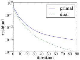
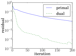
Figure 9: Primal residual $\|r_{\mathrm{p}}^{(k)}\|_{2}/\|\tilde{x}^{(k)}\|_{2}$ and dual residual $\|r_{\mathrm{d}}^{(k)}\|_{2}/\|v^{(k)}\|_{2}$ versus iteration number $k$ for three constant values of $\sigma_{k}$: $\sigma_{k}=0.1$ (left), $\sigma_{k}=0.01$ (middle), and $\sigma_{k}=0.001$ (right).

As can be seen, the choice of $\sigma_{k}$ has a strong effect on the speed of convergence. The figures suggest that when $\sigma_{k}$ is too large (the steplength $1/\sigma_{k}$ is too small) the dual residual decreases more slowly than the primal residual, and when $\sigma_{k}$ is too small, the primal residual decreases more slowly. For a good value of $\sigma_{k}$ in between, the two residuals decrease at about the same rate.

This observation motivates the adaptive strategy (31). Figure 10 shows the residuals if the adaptive strategy is used, with $\mu=2$, $\tau_{k}=1+0.9^{k}$, and starting at three different values of $\sigma_{k}$ ($0.1$, $0.01$, $0.001$). Figure 10 shows the resulting values of $\sigma_{k}$ versus the iteration number $k$.

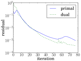
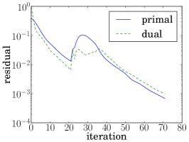
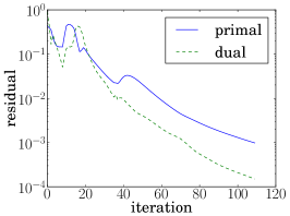
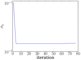
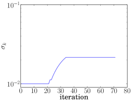
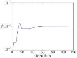
Figure 10: Primal and dual residuals versus iteration number with adaptive selection of $\sigma_{k}$, starting with a value $0.1$ (top left), $0.01$ (middle), $0.001$ (right). The graphs on the bottom row show the values of $\sigma_{k}$ during the three runs of the algorithm.

The convergence graphs indicate that a simple heuristic for adapting the steplength can improve the speed of convergence and make it less dependent on the initial steplength. The specific convergence behavior depends on the parameter $\mu$ and the decay rule for $\tau_{k}$, but is much less sensitive to the choice of $\sigma_{0}$. While in general the convergence with adaptive steplength is not faster than with a carefully tuned constant steplength, the adaptive strategy is more robust than picking an arbitrary constant steplength.

6.2 Approximate Euclidean distance matrix completion

A Euclidean distance matrix (EDM) $D$ is a matrix with entries that can be expressed as squared pairwise distances $D_{ij}=\|x_{i}-x_{j}\|_{2}^{2}$ for some set of vectors $x_{k}$. In this section, we consider the problem of fitting a Euclidean distance matrix to measurements $\widehat{D}_{ij}$ of a subset of its entries. This and related problems arise in many applications, including, for example, the sensor network node localization problem [CY07, KKW09, KW12].

Expanding the identity in the definition of Euclidean distance matrix,

$$D_{ij}=\|x_{i}-x_{j}\|_{2}^{2}=x_{i}^{T}x_{i}-2x_{i}^{T}x_{j}+x_{j}^{T}x_{j},$$

shows that a matrix $D$ is a Euclidean distance matrix if and only if $D_{ij}=X_{ii}-2X_{ij}+X_{jj}$ for a positive semidefinite matrix $X$ (the Gram matrix with entries $X_{ij}=x_{i}^{T}x_{j}$). Furthermore, since $D$ only depends on the pairwise distances of the configuration points, we can arbitrarily place one of the points at the origin or, equivalently, set one row and column of $X$ to zero. This gives an equivalent characterization: $D$ is a $(p+1)\times(p+1)$ Euclidean distance matrix if and only if there exists a positive semidefinite matrix $X\in{\mbox{\bf S}}^{p}$ such that

$$D_{ij}=\mathop{\bf tr}(F_{ij}X),\quad 1\leq i<j\leq p+1$$

where

$$F_{ij}=\left\{\begin{array}[]{ll}(e_{i}-e_{j})(e_{i}-e_{j})^{T}&1\leq i<j\leq p\\ e_{i}e_{i}^{T}&1\leq i<j=p+1\end{array}\right.$$

and $e_{i}$ denotes the $i$th unit vector in ${\mbox{\bf R}}^{p}$.

In the EDM approximation problem we are given a set of measurements $\widehat{D}_{ij}$ for entries $(i,j)\in W$ where

$$W\subseteq\{(i,j)\mid 1\leq i<j\leq p+1\}.$$

The problem of fitting a Euclidean distance matrix to the measurements can be posed as

$$\begin{array}[]{ll}\mbox{minimize}&\sum\limits_{(i,j)\in W}|\mathop{\bf tr}(F_{ij}X)-\widehat{D}_{ij}|\\[12.91663pt] \mbox{subject to}&X\succeq 0,\end{array}$$ (46)

with variable $X\in{\mbox{\bf S}}^{p}$. (We choose the $\ell_{1}$-norm to measure the quality of the fit simply because the problem is more easily expressed as a conic LP.) Now let $V$ be a chordal sparsity pattern of order $p$ that includes the aggregate sparsity pattern of the matrices $F_{ij}$. In other words, if $(i,j)\in W$ with $1\leq i<j\leq p$, then $(i,j)$ is a nonzero in $V$. Moreover $V$ is chordal and includes all the diagonal entries in its nonzeros. Such a pattern $V$ is called a chordal embedding of $W$. Then, without loss of generality, we can restrict the variable $X$ in (46) to be a sparse matrix in ${\mbox{\bf S}}^{p}_{V}$ and we obtain the equivalent problem

$$\begin{array}[]{ll}\mbox{minimize}&\sum\limits_{(i,j)\in W}|\mathop{\bf tr}(F_{ij}X)-\widehat{D}_{ij}|\\[12.91663pt] \mbox{subject to}&X\in{\mbox{\bf S}}^{p}_{{V},\mathrm{c}}.\end{array}$$ (47)

This problem is readily converted into a standard conic LP of the form (34), which can then be solved using the decomposition method of section 5. An interesting feature of this application is that the correlative sparsity associated with the converted problem is block-diagonal.

The conversion method and the block-diagonal correlative sparsity can also be explained directly in terms of the problem (47). Suppose $V$ has $l$ cliques $\beta_{k}$, $k=1,\ldots,l$. Suppose we partition the set $W$ in $l$ sets $W_{k}$ with the property that if $(i,j)\in W_{k}$ and $1\leq i<j\leq p$, then $i,j\in\beta_{k}$, and if $(i,p+1)\in W_{k}$, then $i\in\beta_{k}$. Then (47) is equivalent to

$$\begin{array}[]{ll}\mbox{minimize}&\sum\limits_{k=1}^{l}\sum\limits_{(i,j)\in W_{k}}|\mathop{\bf tr}(F_{ij}\mathcal{E}_{\beta_{k}}^{*}(\tilde{X}_{k}))-\widehat{D}_{ij}|\\[12.91663pt] \mbox{subject to}&\mathcal{E}_{\eta_{j}}(\mathcal{E}_{\beta_{k}}^{*}(\tilde{X}_{k})-\mathcal{E}_{\beta_{j}}^{*}(\tilde{X}_{j}))=0,\quad k=1,\ldots,l,\quad\beta_{j}\in\mathop{\mathrm{ch}}(\beta_{k})\\[4.30554pt] &\tilde{X}_{k}\succeq 0,\quad k=1,\ldots,l,\end{array}$$ (48)

with variables $\tilde{X}_{k}\in{\mbox{\bf S}}^{|\beta_{k}|}$, $k=1,\ldots,l$. This problem can be solved using Spingarn’s method. At each iteration we alternate between projection on the subspace defined by the consistency equations in (48) and evaluation of a prox-operator, via the solution of

$$\begin{array}[]{ll}\mbox{minimize}&\sum\limits_{k=1}^{l}\sum\limits_{(i,j)\in W_{k}}|\mathop{\bf tr}(F_{ij}\mathcal{E}_{\beta_{k}}^{*}(\tilde{X}_{k}))-\widehat{D}_{ij}|+(\sigma/2)\sum\limits_{k=1}^{l}\|\tilde{X}_{k}-Z_{k}\|_{F}^{2}\\[12.91663pt] \mbox{subject to}&\tilde{X}_{k}\succeq 0,\quad k=1,\ldots,l.\end{array}$$ (49)

Note that this problem is separable because if $(i,j)\in W_{k}$, $F_{ij}$ is nonzero only in positions that are included in $\beta_{k}\times\beta_{k}$. The problems (49) can be solved efficiently via a straightforward modification of the interior-point method described in section 5.2.

We now illustrate the convergence of the decomposition method on two randomly generated networks. An example of a network topology is shown in Figure 11 for a problem with 500 nodes.

\psfrag{t}{}\includegraphics[width=195.12767pt]{network_psfrag.eps}

Figure 11: Nearest-neighbor network for a problem with $500$ nodes in two dimensions. Two nodes are connected if one of the two is among the 5 nearest neighbors of the other node.

The network edges are assigned using the following rule: a pair $(i,j)$ is in the sparsity pattern $W$ if one of the nodes is among the five nearest neighbors of the other node.

To compute a chordal embedding $V$, we use an approximate minimum degree (AMD) reordering, which gives a permutation of the sparsity pattern that reduces fill-in (Figure 12, left). Often, the resulting embedding contains many small cliques and for our purposes it is more efficient to merge some neighboring cliques, using algorithms similar to those in [AG89, RS09, HS10]. Specifically, traversing the tree in a topological order, we greedily merge clique $k$ with its parent if

$$(|\beta_{\mathop{\mathrm{pa}}(k)}|-|\eta_{k}|)(|\beta_{k}|-|\eta_{k}|)\leq t_{\mathrm{fill}}\quad\text{or}\quad\max(|\beta_{k}|-|\eta_{k}|,|\beta_{\mathop{\mathrm{pa}}(k)}|-|\eta_{\mathop{\mathrm{pa}}(k)}|)\leq t_{\mathrm{size}}$$

where $t_{\mathrm{fill}}$ is a threshold based on the amount of fill that results from merging clique $k$ with its parent, and $t_{\mathrm{size}}$ is a threshold based on the cardinality of the sets $\beta_{\mathop{\mathrm{pa}}(k)}\setminus\eta_{\mathop{\mathrm{pa}}(k)}$ and $\beta_{k}\setminus\eta_{k}$. In Figure 12 (right) we show the result of this clique-merging technique using the values $t_{\mathrm{fill}}=t_{\mathrm{size}}=5$. This reduced the 359 original cliques with an average of 5 nodes each to 79 cliques with an average of 10 nodes.

\psfrag{t}{}\includegraphics[width=173.44534pt]{amd_psfrag.eps}

\psfrag{t}{}\includegraphics[width=173.44534pt]{cliquemerging_psfrag.eps}

Figure 12: Sparsity pattern for a network with 500 nodes after approximate minimum degree (AMD) reordering and chordal embedding (left), and after clique merging (right). Before clique merging, there are 359 cliques with an average of 5 elements. After clique merging, there are 79 cliques with an average of 5 elements.

A typical convergence plot of the resulting problem is given in Figure 13 for a network with 500 nodes (left) and 2000 nodes (right). A constant value $\sigma_{k}=5.0$ is used for the steplength parameter. The greedy clique merging strategy described above was used, with the same threshold values.

\psfrag{t}{}\psfrag{x}[t][t]{iteration}\psfrag{z}[b][b]{residual}\includegraphics[width=208.13574pt]{evolution_N500_psfrag.eps}

\psfrag{t}{}\psfrag{x}[t][t]{iteration}\psfrag{z}[b][b]{residual}\includegraphics[width=208.13574pt]{evolution_N2000_psfrag.eps}

Figure 13: Relative primal and dual residuals versus iteration number for networks with 500 (upper left) and 2000 (right) nodes. For $n=500$, there are 82 cliques, and for $n=2000$, there are 310 cliques. A constant steplength parameter $\sigma_{k}=5.0$ is used.

6.3 Block-arrow semidefinite programs

In the last experiment we compare the efficiency of the splitting method with general-purpose SDP solvers. We consider a family of randomly generated SDPs with a block-arrow aggregate sparsity pattern $V$ and a block-diagonal correlative sparsity pattern. The sparsity pattern $V$ is defined in Figure 14.

Figure 14: Block arrow pattern with $l$ cliques and corresponding clique tree. The order of the matrix is $ld+w$. The first $l$ diagonal blocks in the matrix have size $d$, the last block column and block row have width $w$. The cliques therefore have size $d+w$. Each clique in the clique tree is partitioned in two sets: the top row shows $\eta_{k}=\beta_{k}\cap\mathop{\mathrm{pa}}(\beta_{k})$; the bottom row shows $\beta_{k}\setminus\eta_{k}$.

It consists of $l$ diagonal blocks of size $d\times d$, plus $w$ dense final rows and columns. We take the clique

$$\beta_{l}=\{(l-1)d+1,\,\ldots,\,ld,\,ld+1,\,\ldots,\,ld+w\}$$

(with $\eta_{l}=\{\}$) as root of the clique tree. The other $l-1$ cliques $\beta_{k}$ and the intersections $\eta_{k}=\beta_{k}\cap\mathop{\mathrm{pa}}(\beta_{k})$ with their parent cliques are

$$\beta_{k}=\{(k-1)d+1,\,\ldots,\,kd\}\cup\eta_{k},\qquad\eta_{k}=\{ld+1,ld+2,\ldots,ld+w\},\qquad k=1,\ldots,l-1.$$

We generate matrix cone LPs (34) with $m=ls$ primal equality constraints, partitioned in $l$ sets

$$\nu_{k}=\{(k-1)s+1,\,(k-1)s+2,\,\ldots,\,ks\},\qquad k=1,\ldots,l,$$

of equal size $|\nu_{k}|=s$. If $i\in\nu_{k}$, then the coefficient matrix $F_{i}$ contains a dense $\beta_{k}\times\beta_{k}$ block, and is otherwise zero. We will use the notation

$$(F_{i})_{\beta_{k}\beta_{k}}=\left[\begin{array}[]{cc}A_{i}&B_{i}\\ B_{i}^{T}&D_{i}\end{array}\right],$$

for the nonzero block of $F_{i}$ if $i\in\nu_{k}$. The primal and dual SDPs can therefore be expressed as

$$\begin{array}[t]{ll}\mbox{minimize}&\mathop{\bf tr}(CX)\\ \mbox{subject to}&\mathcal{A}(X)=b\\ &X\succeq 0\end{array}\qquad\qquad\begin{array}[t]{ll}\mbox{maximize}&b^{T}y\\ \mbox{subject to}&\mathcal{A}^{*}(y)+S=C\\ &S\succeq 0\end{array}$$ (50)

with a linear mapping $\mathcal{A}:{\mbox{\bf S}}^{(ld+w)\times(ld+w)}\rightarrow{\mbox{\bf R}}^{ls}$ defined as

$$\mathcal{A}(X)_{i}=\mathop{\bf tr}\left(\left[\begin{array}[]{cc}A_{i}&B_{i}\\ B_{i}^{T}&D_{i}\end{array}\right]\left[\begin{array}[]{cc}X_{kk}&X_{k,l+1}\\ X_{l+1,k}&X_{l+1,l+1}\end{array}\right]\right),\quad i\in\nu_{k},\quad k=1,\ldots,l,$$

where $X_{ij}$ denotes the $i,j$ block of $X$. (These blocks have dimensions $X_{ii}\in{\mbox{\bf S}}^{d}$ for $i=1,\ldots,l$, $X_{l+1,l+1}\in{\mbox{\bf S}}^{w}$, $X_{l+1,i}\in{\mbox{\bf R}}^{w\times d}$ for $i=1,\ldots,l$.) The adjoint $\mathcal{A}^{*}:{\mbox{\bf R}}^{ls}\rightarrow{\mbox{\bf S}}^{(ld+w)\times(ld+w)}$ is

$$\mathcal{A}^{*}(y)=\left[\begin{array}[]{ccccc}\sum\limits_{i\in\nu_{1}}y_{i}A_{i}&0&\cdots&0&\sum\limits_{i\in\nu_{1}}y_{i}B_{i}\\ 0&\sum\limits_{i\in\nu_{2}}y_{i}A_{i}&\cdots&0&\sum\limits_{i\in\nu_{2}}y_{i}B_{i}\\ \vdots&\vdots&\ddots&\vdots&\vdots\\ 0&0&\cdots&\sum\limits_{i\in\nu_{l}}y_{i}A_{i}&\sum\limits_{i\in\nu_{l}}y_{i}B_{i}\\ \sum\limits_{i\in\nu_{1}}y_{i}B_{i}^{T}&\sum\limits_{i\in\nu_{2}}y_{i}B_{i}^{T}&\cdots&\sum\limits_{i\in\nu_{l}}y_{i}B_{i}^{T}&\sum\limits_{i=1}^{m}y_{i}D_{i}\end{array}\right].$$

In the reformulated problem, the variable $X$ is replaced with $l$ matrices $\tilde{X}_{k}=X_{\beta_{k}\beta_{k}}$, i.e., defined as

$$\tilde{X}_{k}=\left[\begin{array}[]{cc}(\tilde{X}_{k})_{11}&(\tilde{X}_{k})_{12}\\ (\tilde{X}_{k})_{21}&(\tilde{X}_{k})_{22}\end{array}\right]=\left[\begin{array}[]{cc}X_{kk}&X_{k,l+1}\\ X_{k,l+1}^{T}&X_{l+1,l+1}\end{array}\right],\quad k=1,\ldots,l,$$

and the primal SDP is converted to

$$\begin{array}[]{ll}\mbox{minimize}&\sum\limits_{k=1}^{l}\mathop{\bf tr}(\tilde{C}_{k}\tilde{X}_{k})\\ \mbox{subject to}&\mathop{\bf tr}\left(\left[\begin{array}[]{cc}A_{i}&B_{i}\\ B_{i}^{T}&D_{i}\end{array}\right]\left[\begin{array}[]{cc}(\tilde{X}_{k})_{11}&(\tilde{X}_{k})_{12}\\ (\tilde{X}_{k})_{21}&(\tilde{X}_{k})_{22}\end{array}\right]\right)=b_{i},\quad i\in\nu_{k},\quad k=1,\ldots,l\\[8.61108pt] &(\tilde{X}_{k})_{22}=(\tilde{X}_{l})_{22},\quad k=1,\ldots,l-1\\ &\tilde{X}_{k}\succeq 0,\quad k=1,\ldots,l\end{array}$$ (51)

where

$$\tilde{C}_{k}=\left[\begin{array}[]{cc}C_{kk}&C_{k,l+1}\\ C_{k,l+1}^{T}&0\end{array}\right],\quad k=1,\ldots,l-1,\qquad\tilde{C}_{l}=\left[\begin{array}[]{cc}C_{ll}&C_{l,l+1}\\ C_{l,l+1}^{T}&C_{l+1,l+1}\end{array}\right].$$

With this choice of parameters, the correlative sparsity pattern of the converted SDP (51) is block-diagonal, i.e., except for the consistency constraints $(\tilde{X}_{k})_{22}=(\tilde{X}_{l})_{22}$ the problem is separable with independent variables $\tilde{X}_{k}\in{\mbox{\bf S}}^{p+w}$. This allows us to compute the prox-operator by solving $l$ independent conic QPs.

Problem generation

The problem data are randomly generated as follows. First, the entries of $A_{k}$, $B_{k}$, $D_{k}$ are drawn independently from a normal distribution $\mathcal{N}(0,1)$. A strictly primal feasible $X$ is constructed as $X=W+\alpha I$ where $W\in{\mbox{\bf S}}^{p}_{V}$ is randomly generated with i.i.d. entries from $\mathcal{N}(0,1)$ and $\alpha$ is chosen so that $X_{\beta_{k}\beta_{k}}=W_{\beta_{k}\beta_{k}}+\alpha I\succ 0$ for $k=1,\ldots,l$. The right-hand side $b$ in the primal constraint is computed as $b_{i}=\mathop{\bf tr}(F_{i}X)$, $i=1,\ldots,m$.

Next, strictly dual feasible $y\in{\mbox{\bf R}}^{m}$, $S\in{\mbox{\bf S}}^{p}_{V}$ are constructed. The vector $y$ has i.i.d. entries from $\mathcal{N}(0,1)$ and $S$ is constructed as $S=\sum_{k=1}^{l}\mathcal{E}^{*}_{\beta_{k}}(\tilde{S}_{k})$, with $\tilde{S}_{k}=W_{k}+\alpha I$, $W_{k}\in{\mbox{\bf S}}^{|\beta_{k}|}$ randomly generated with i.i.d. $\mathcal{N}(0,1)$ entries, and $\alpha$ chosen so that $\tilde{S}_{k}\succ 0$. Finally, the matrix $C$ is constructed as $C=S+\sum_{i}y_{i}F_{i}$.

Comparison with general-purpose SDP solvers

In Figure 15 we compare the solution time of Spingarn’s algorithm with the general-purpose interior-point solvers SEDUMI and SDPT3, applied to the unconverted and converted SDPs (33) and (38).

\psfrag{z}[b][b]{time (sec)}\psfrag{t}{}\psfrag{x}[t][t]{$w$ (arrow width)}\includegraphics[width=212.47617pt]{arrowwidth_psfrag.eps}

\psfrag{z}[b][b]{time (sec)}\psfrag{t}{}\psfrag{x}[t][t]{$l$ (number of cliques)}\includegraphics[width=212.47617pt]{cliques_psfrag.eps}

Figure 15: Solution time for randomly generated SDPs with block-arrow sparsity patterns. Times are reported for SEDUMI (SED.) and SDPT3 applied to the original (‘unc.’) and converted (‘conv’) SDPs, and the Spingarn method applied to the converted SDP. The figure on the left shows the times as function of arrow width $w$, for fixed dimensions $l=100$, $d=20$, $s=10$. The figure on the right shows the times versus number of cliques $l$, for fixed dimensions $w=20$, $d=20$, $s=10$.

In the decomposition method we use a constant steplength parameter $\sigma_{k}=5$ and relaxation parameter $\rho_{k}=1.75$. The stopping criterion is (30) with $\epsilon_{\mathrm{p}}=\epsilon_{\mathrm{d}}=10^{-4}$. For each data point we report the average CPU time over 5 instances.

To interpret the results, it is useful to consider the linear algebra complexity per iteration of each method. The unconverted SDP (50) has a single matrix variable $X$ of order $p=ld+w$. The cost per iteration of an interior-point method is dominated by the cost of forming and solving the Schur complement equation, which is dense and of size $m=sl$. For the problem sizes used in the figures ($w$ small compared to $ld$) the cost of solving the Schur complement dominates the overall complexity. This explains the nearly constant solution time in the first figure (fixed $l$, $s$, $p$, varying $w$) and the increase with $l$ shown in the second figure.

The converted SDP (51) has $l$ variables $\tilde{X}_{k}$ of order $d+w$. The Schur complement equation in an interior-point method has the general structure (20) with a leading block-diagonal matrix ($l$ blocks of size $s\times s$) augmented with a dense block row and block column of width proportional to $lw^{2}$. For small $w$, exploiting the block-diagonal structure in the Schur complement equation, allows one to solve the Schur complement equation very quickly and reduces the cost per iteration to a fraction of a cost of solving the unconverted problem, despite the increased size of the problem. However the advantage disappears with increasing $w$ (Figure 15 left).

The main step in each iteration of the Spingarn method applied to the converted problem is the evaluation of the prox-operators via an interior-point method. The Schur complement equations that arise in this computation are block-diagonal ($l$ blocks of order $s$) and therefore the cost of solving them is independent of $w$ and linear in $l$. As an additional advantage, since the correlative sparsity pattern is block-diagonal, the proximal operator can be evaluated by solving $l$ independent conic QPs that can be solved in parallel. This was not implemented in the experiment, but could reduce the solution time by a factor of roughly $l$.

Accuracy and steplength selection

The principal disadvantage of the splitting method, compared with an interior-point method, is the more limited accuracy and the higher sensitivity to the choice of algorithm parameters. Figure 16 (left) shows the number of iterations versus $l$ for different values of the tolerance $\epsilon$ used in the stopping criterion.

\psfrag{x}[t][t]{$l$ (number of cliques)}\psfrag{z}[b][b]{number of iterations}\psfrag{t}{}\includegraphics[width=212.47617pt]{accuracy_iter_psfrag.eps}

\psfrag{x}[t][t]{$l$ (number of cliques)}\psfrag{z}[b][b]{number of iterations}\psfrag{t}{}\includegraphics[width=212.47617pt]{adaptive_iter_psfrag.eps}

Figure 16: Left. Number of iterations for of Spingarn’s method based on the desired accuracy, for a problem instance with $d=20$, $w=20$, $s=10$, and using a fixed steplength parameter $\sigma_{k}=5$. Right. Number of iterations for the same problem with $\epsilon=10^{-4}$ and different choices of steplength.

The right-hand plot shows the number of iterations versus $l$ for two different constant values of the steplength parameter $\sigma_{k}$ ($\sigma_{k}=1.0$ and $\sigma_{k}=5.0$) and for an adaptively adjusted steplength.

7 Conclusions

We have described a decomposition method that exploits partially separable structure in linear conic optimization problems. The basic idea is straightforward: by replicating some of the variables, we reformulate the problem as an equivalent linear optimization problem with block-separable conic inequalities and an equality constraint that ensures that the replicated variables are consistent. We can then apply Spingarn’s method of partial inverses to this equality-constrained convex problem. Spingarn’s method is a generalized alternating projection method for convex optimization over a subspace. It alternates orthogonal projections on the subspace with the evaluation of the proximal operator of the cost function. In the method described in the paper, these prox-operators are evaluated by an interior-point method for conic quadratic optimization.

When applied to sparse semidefinite programs, the reformulation coincides with the clique conversion methods which were introduced in [KKMY11, FKMN00] with the purpose of exploiting sparsity in interior-point methods for semidefinite programming. By solving the converted problems via a splitting algorithm instead of an interior-point algorithm we extend the applicability of the conversion methods to problems for which the converted problem is too large to handle by interior-point methods. As a second advantage, if the correlative sparsity is block-diagonal, the most expensive step of the decomposition algorithm (the evaluation of the proximal operator) becomes separable and can be parallelized. The numerical experiments indicate that the approach is effective when a moderate accuracy (compared with interior-point methods) is acceptable. However the convergence can be quite slow and strongly depends on the choice of steplength.

A critical component in the decomposition algorithm for semidefinite programming is the use of a customized interior-point method for evaluating the proximal operators. This technique allows us to evaluate the proximal operator at roughly the same cost of solving the reformulated SDP without the consistency constraints. As a further improvement we hope to extend this technique to exploit sparsity in the coefficient matrices of the reformulated problem, using techniques developed for interior-point methods for sparse matrix cones [ADV12].

While sparse semidefinite programming provides the most important application of our results, the techniques easily extend to other types of partially separable cones. In many of these extensions partial separability does not require chordal structure (as it does in semidefinite programming). As an example, second-order cone programs with partially separable structure arise in machine learning problems involving sum-of-norm penalties that promote group sparsity [BJMO11].

References

- [ADLV12] M. S. Andersen, J. Dahl, Z. Liu, and L. Vandenberghe. Interior-point methods for large-scale cone programming. In S. Sra, S. Nowozin, and S. J. Wright, editors, Optimization for Machine Learning, pages 55–83. MIT Press, 2012.
- [ADV10a] M. Andersen, J. Dahl, and L. Vandenberghe. CVXOPT: A Python Package for Convex Optimization. www.cvxopt.org, 2010.
- [ADV10b] M. S. Andersen, J. Dahl, and L. Vandenberghe. Implementation of nonsymmetric interior-point methods for linear optimization over sparse matrix cones. Mathematical Programming Computation, 2:167–201, 2010.
- [ADV12] M. S. Andersen, J. Dahl, and L. Vandenberghe. Logarithmic barriers for sparse matrix cones. Optimization Methods and Software, 2012.
- [AG89] C. Ashcraft and R. Grimes. The influence of relaxed supernode partitions on the multifrontal method. ACM Transactions on Mathematical Software, 15(4):291–309, 1989.
- [AHMR88] J. Agler, J. W. Helton, S. McCullough, and L. Rodman. Positive semidefinite matrices with a given sparsity pattern. Linear Algebra and Its Applications, 107:101–149, 1988.
- [BC11] H. H. Bauschke and P. L. Combettes. Convex Analysis and Monotone Operator Theory in Hilbert Spaces. Springer, 2011.
- [BJMO11] F. Bach, R. Jenatton, J. Mairal, and G. Obozinski. Optimization with sparsity-inducing penalties. Foundations and Trends in Machine Learning, 4(1):1–106, 2011.
- [BP93] J. R. S. Blair and B. Peyton. An introduction to chordal graphs and clique trees. In A. George, J. R. Gilbert, and J. W. H. Liu, editors, Graph Theory and Sparse Matrix Computation. Springer-Verlag, 1993.
- [BT97] D. P. Bertsekas and J. N. Tsitsiklis. Parallel and Distributed Computation: Numerical Methods. Athena Scientific, Belmont, Mass., 1997.
- [Bur03] S. Burer. Semidefinite programming in the space of partial positive semidefinite matrices. SIAM Journal on Optimization, 14(1):139–172, 2003.
- [BV04] S. Boyd and L. Vandenberghe. Convex Optimization. Cambridge University Press, Cambridge, 2004. www.stanford.edu/~boyd/cvxbook.
- [CP07] P. L. Combettes and J.-C. Pesquet. A Douglas-Rachford splitting approach to nonsmooth convex variational signal recovery. IEEE Journal of Selected Topics in Signal Processing, 1(4):564–574, 2007.
- [CY07] A. M.-C. Cho and Y. Ye. Theory of semidefinite programming for sensor network localization. Mathematical Programming, Series B, 109:367–384, 2007.
- [DZG12] E. Dall’Anese, H. Zhu, and G. B. Giannakis. Distributed optimal power flow for smart microgrids. 2012. arxiv.org/1211.5856.
- [EB92] J. Eckstein and D. Bertsekas. On the Douglas-Rachford splitting method and the proximal point algorithm for maximal monotone operators. Mathematical Programming, 55:293–318, 1992.
- [Eck94] J. Eckstein. Parallel alternating direction multiplier decomposition of convex programs. Journal of Optimization Theory and Applications, 80(1):39–62, 1994.
- [FKMN00] M. Fukuda, M. Kojima, K. Murota, and K. Nakata. Exploiting sparsity in semidefinite programming via matrix completion I: general framework. SIAM Journal on Optimization, 11:647–674, 2000.
- [GB08] M. Grant and S. Boyd. Graph implementations for nonsmooth convex programs. In V. Blondel, S. Boyd, and H. Kimura, editors, Recent Advances in Learning and Control (a tribute to M. Vidyasagar), pages 95–110. Springer, 2008.
- [GB11] M. Grant and S. Boyd. CVX: Matlab Software for Disciplined Convex Programming, version 1.21. cvxr.com, 2011.
- [GJSW84] R. Grone, C. R. Johnson, E. M Sá, and H. Wolkowicz. Positive definite completions of partial Hermitian matrices. Linear Algebra and Appl., 58:109–124, 1984.
- [GT82] A. Griewank and Ph. L. Toint. Partitioned variable metric updates for large structured optimization problems. Numerische Mathematik, 39:119–137, 1982.
- [GT84] A. Griewank and Ph. L. Toint. On the existence of convex decompositions of partially separable functions. Mathematical Programming, 28:25–49, 1984.
- [HLW03] B. S. He, L. Z. Liao, and S. L. Wang. Self-adaptive operator splitting methods for monotone variational inequalities. Numerische Mathematik, 94:715–737, 2003.
- [HS10] J. Hogg and J. Scott. A modern analyse phase for sparse tree-based direct methods. Technical report, 2010.
- [HYW00] B. S. He, H. Yang, and S. L. Wang. Alternating direction method with self-adaptive penalty parameters for monotone variational inequalities. Journal of Optimization Theory and Applications, 106:337–356, 2000.
- [KKK08] K. Kobayashi, S. Kim, and M. Kojima. Correlative sparsity in primal-dual interior-point methods for LP, SDP, and SOCP. Applied Mathematics and Optimization, 58(1):69–88, 2008.
- [KKMY11] S. Kim, M. Kojima, M. Mevissen, and M. Yamashita. Exploiting sparsity in linear and nonlinear matrix inequalities via positive semidefinite matrix completion. Mathematical Programming, 129:33–68, 2011.
- [KKW09] S. Kim, M. Kojima, and H. Waki. Exploiting sparsity in SDP relaxations for sensor network localization. SIAM Journal on Optimization, 20(1):192–215, 2009.
- [KW12] N. Krislock and H. Wolkowicz. Euclidean distance matrices and applications. In M. F. Anjos and J. B. Lasserre, editors, Handbook of Semidefinite, Cone and Polynomial Optimization: Theory, Algorithms, Software and Applications, volume 166 of International Series in Operations Research & Management Science, pages 879–914. Springer, Waterloo, Ontario, 2012.
- [Las02] L. S. Lasdon. Optimization Theory for Large Systems. Dover Publications, Inc., 2002. First published in 1970 by the MacMillan Company.
- [LM79] P. L. Lions and B. Mercier. Splitting algorithms for the sum of two nonlinear operators. SIAM Journal on Numerical Analysis, 16(6):964–979, 1979.
- [LNM07] Z. Lu, A. Nemirovski, and R. D. C. Monteiro. Large-scale semidefinite programming via a saddle-point Mirror-Prox algorithm. 109:211–237, 2007.
- [LPP89] J. G. Lewis, B. W. Peyton, and A. Pothen. A fast algorithm for reordering sparse matrices for parallel factorization. SIAM Journal on Scientific and Statistical Computing, 10(6):1146–1173, 1989.
- [Mor65] J. J. Moreau. Proximité et dualité dans un espace hilbertien. Bull. Math. Soc. France, 93:273–299, 1965.
- [NFF+03] K. Nakata, K. Fujitsawa, M. Fukuda, M. Kojima, and K. Murota. Exploiting sparsity in semidefinite programming via matrix completion II: implementation and numerical details. Mathematical Programming Series B, 95:303–327, 2003.
- [NW06] J. Nocedal and S. J. Wright. Numerical Optimization. Springer, 2nd edition, 2006.
- [NWV08] M. Nouralishahi, C. Wu, and L. Vandenberghe. Model calibration for optical lithography via semidefinite programming. Optimization and Engineering, 9:19–35, 2008.
- [PB12] N. Parikh and S. Boyd. Graph projection block splitting for distributed optimization. 2012. Submitted.
- [PS90] A. Pothen and C. Sun. Compact clique tree data structures in sparse matrix factorizations. In T. F. Coleman and Y. Li, editors, Large-Scale Numerical Optimization, pages 180–204. Society for Industrial and Applied Mathematics, 1990.
- [RS09] J. K. Reid and J. A. Scott. An out-of-core sparse cholesky solver. ACM Transactions on Mathematical Software, 36(2):133, 2009.
- [Spi83] J. E. Spingarn. Partial inverse of a monotone operator. Applied Mathematics and Optimization, 10:247–265, 1983.
- [Spi85] J. E. Spingarn. Applications of the method of partial inverses to convex programming: decomposition. Mathematical Programming, 32:199–223, 1985.
- [Stu99] J. F. Sturm. Using SEDUMI 1.02, a Matlab toolbox for optimization over symmetric cones. Optimization Methods and Software, 11-12:625–653, 1999.
- [SV04] G. Srijuntongsiri and S. Vavasis. A fully sparse implementation of a primal-dual interior-point potential reduction method for semidefinite programming. 2004. arXiv:cs/0412009.
- [TTT07] K. C. Toh, R. H. Tütüncü, and M. J. Todd. Inexact primal-dual path-following algorithms for a special class of convex quadratic SDP and related problems. Pacific Journal of Optimization, 3, 2007.
- [TY84] R. E. Tarjan and M. Yannakakis. Simple linear-time algorithms to test chordality of graphs, test acyclicity of hypergraphs, and selectively reduce acyclic hypergraphs. SIAM Journal on Computing, 13(3):566–579, 1984.
- [WL01] S. L. Wang and L. Z. Liao. Decomposition method with a variable parameter for a class of monotone variational inequality problems. Journal of Optimization Theory and Applications, 109(2):415–429, 2001.