Numerical Treatment of Anisotropic Radiation Field Coupling with the Relativistic Resistive Magnetofluids

Abstract

We develop a numerical scheme for solving a fully special relativistic resistive radiation magnetohydrodynamics. Our code guarantees conservations of total mass, momentum and energy. Radiation energy density and radiation flux are consistently updated using the M-1 closure method, which can resolve an anisotropic radiation fields in contrast to the Eddington approximation as well as the flux-limited diffusion approximation. For the resistive part, we adopt a simple form of the Ohm’s law. The advection terms are explicitly solved with an approximate Riemann solver, mainly HLL scheme, and HLLC and HLLD schemes for some tests. The source terms, which describe the gas-radiation interaction and the magnetic energy dissipation, are implicitly integrated, relaxing the Courant-Friedrichs-Lewy condition even in optically thick regime or a large magnetic Reynolds number regime. Although we need to invert $4\times 4$ (for gas-radiation interaction) and $3\times 3$ (for magnetic energy dissipation) matrices at each grid point for implicit integration, they are obtained analytically without preventing massive parallel computing. We show that our code gives reasonable outcomes in numerical tests for ideal magnetohydrodynamics, propagating radiation, and radiation hydrodynamics. We also applied our resistive code to the relativistic Petschek type magnetic reconnection, revealing the reduction of the reconnection rate via the radiation drag.

1. Introduction

Radiation and/or magnetic fields, relativity, and resistivity play crucial roles in a number of high-energy astrophysical phenomena, such as black-hole accretion-disks, jets, disk winds, pulsar winds, magnetar flares, core collapse supernovae, and gamma-ray bursts. For example, the geometrically thick disk is supported by the radiation pressure, which dominates the total pressure, in the case of near- or super-critical accretion rate. The radiation force is thought to accelerate the matter, producing jets or winds (Lynden-Bell, 1978; Icke, 1980, 1989; Tajima & Fukue, 1996). In contrast, the radiation drag reduces the velocity of the relativistic outflow. The magnetic field lines enhanced in the inner part of the accretion disks launch jets/outflows (Blandford & Payne, 1982; Uchida & Shibata, 1985; Kudoh & Shibata, 1997). The magnetorotational instability (MRI) is thought to be origin of the disk viscosity, by which the angular momentum is transported outward (Velikhov, 1959; Chandrasekhar, 1960; Balbus & Hawley, 1991). The resistivity would cause conversion from the magnetic energy to the energy of the matter through the magnetic reconnection. Also, the resistivity might influence the evolution and/or saturation of MRI in the disks (Lesur & Longaretti, 2007; Fromang et al., 2007; Simon & Hawley, 2009; Fromang et al., 2012).

A global structure of the accretion disks and outflows is investigated by radiation hydrodynamics (RHD) simulations (Eggum et al., 1987, 1988; Okuda & Fujita, 2000; Ohsuga et al., 2005; Ohsuga, 2006), magnetohydrodynamics (MHD) simulations (Machida et al., 2006; Kato et al., 2008; McKinney & Blandford, 2009; Tchekhovskoy et al., 2010), and Radiation-MHD (RMHD) simulations (Ohsuga et al., 2009; Takeuchi et al., 2010; Ohsuga & Mineshige, 2011). Especially, Takeuchi et al. (2010) showed high-velocity jets, which is magnetically collimated, are powered by the radiation force. Also RMHD simulations of local patch of the disk are performed (Hirose et al., 2009; Jiang et al., 2013). Although such works were great successful, they should extent to relativistic simulations.

Many approximate methods have been proposed to solve the radiation transfer, since the computational cost for rigorous method is too expensive to perform. In the flux-limited diffusion (FLD) approximation, a zeroth moment equation of the radiation transfer equation is solved to update the radiation energy density. The radiation flux as well as the radiation stress tensor is given based on the gradient of the radiation energy density. The FLD is a quite useful technique and gives appropriate radiation fields within the optically thick regime, but it does not always give precise radiation fields in the regime where the optical depth is around unity or less (see Ohsuga & Mineshige, 2011). In contrast to the FLD approximation, both zeroth and first moment equations are solved in the Eddington approximation. However, this method is somewhat problematic for anisotropic radiation fields, since the Eddington tensor is evaluated by assuming the isotropic radiation fields. Additionally, the speed of light is effectively reduced in this method.

Although the variable Eddington tensor method proposed by Stone et al. (1992) is known to give better results, it is so complex and expensive. One of the reasonable method is so-called M-1 closure, in which the Eddington tensor is obtained as a function of the radiation energy density and radiation flux (Minerbo, 1978; Levermore, 1984). The anisotropy of radiation fields is approximately taken into consideration, and the radiation propagates with speed of light in an optically thin medium. The M-1 closure is adopted to non-relativistic radiation hydrodynamic code (González et al., 2007), and recently to general relativistic (GR) code (Sa̧dowski et al., 2013). Another truncated moment formalism of radiation fields in optically thick and thin limits was proposed by Shibata et al. (2011).

Relativistic RMHD or RHD simulations were recently initiated. Farris et al. (2008) first proposed a numerical scheme of GR-RMHD, in which the Eddington approximation is employed. Zanotti et al. (2011) adopted a general relativistic RMHD code to the Bondi-Hoyle accretion on to the black holes. However, in their works, the explicit integration method is employed even for the gas-radiation interaction. In the relativistic phenomena, the dynamical timescale as well as the timescale, that the characteristic wave passes the system, could be comparable to the light crossing time. Thus, although the numerical timestep becomes slightly short via the explicit treatment of the propagating radiation, the computational cost does not increase so much. In contrast, if the absorption/scattering opacity is so large, the timescale of gas-radiation interaction could be much shorter than the other timescales, making the computation to be time consuming. In the non-relativistic RHD/RMHD simulations, such a difficulty is avoided by that the gas-radiation interaction terms are implicitly solved. We should employ such an implicit treatment in the relativistic code (Roedig et al., 2012; Sa̧dowski et al., 2013; Takahashi et al., 2013).

For resistive simulations, the magnetic energy dissipation should be implicitly solved to relax the Courant-Friedrichs-Lewy condition in the regime of a large magnetic Reynolds number. Here note that including the resistivity is a lot more complicated in the relativistic MHD than in the non-relativistic MHD, since we have to solve four additional equations for calculating the time evolution of the electric fields and charge density. The numerical treatment of relativistic MHD simulations with resistivity were developed by authors (Komissarov, 2007; Watanabe & Yokoyama, 2006; Palenzuela et al., 2009; Takamoto & Inoue, 2011). The relativistic resistive RMHD simulations are challenging task.

In the present paper, we propose an explicit-implicit scheme for solving special relativistic RMHD (SR-RMHD) and special relativistic Resistive RMHD (SR-R2MHD) equations. Here, the radiation fields in the observer frame are used and we solve zeroth and first moment equations with the M-1 method. Since the M-1 closure is constructed for the radiation energy momentum tensor to be covariant, the Lorentz transformation for the radiation fields is unnecessary in our procedure. Our scheme ensures a conservation of total energy and momentum (matter, magnetic field, and radiation). An advection of magnetofluids and the radiation is explicitly solved, and the gas-radiation interaction as well as the magnetic energy dissipation via the resistivity is implicitly treated. Note that, although we propose SR code in the present study, the extension to the GR version would be straightforward except for the M-1 closure. The procedure of the M-1 closure in GR code is shown in Shibata et al. (2011).

This paper is organized as follows: In § 2, we introduce argument equations for SR-RMHD and SR-R2MHD. The numerical scheme is explained in § 3, and we show the results in § 4. Finally, § 5 is devoted to summary.

2. Basic Equations

In the following, we take a light speed as unity and assume the Minkowski flat space-time. The metric is described by $\eta^{\mu\nu}=\mathrm{diag}(-1,1,1,1)$. Greek indices range over $0,1,2,3$ and Latin does over $1,2,3$, where $0$ indicates the time component and $1,2,3$ do space components.

A set of equations for the fully special relativistic radiation electro-magnetohydrodynamics consists of conservation of mass,

$$\partial_{\nu}(\rho u^{\nu})=0,$$ (1)

conservation of energy,

$$\partial_{t}\left[\rho h\gamma^{2}-p_{g}+\frac{\mbox{\boldmath$E$}^{2}+\mbox{\boldmath$B$}^{2}}{2}\right]+\nabla\cdot\left[\rho h\gamma u+\mbox{\boldmath$E$}\times\mbox{\boldmath$B$}\right]=G^{0},$$

(2)

conservation of momentum,

$$\partial_{t}\left[\rho h\gamma\mbox{\boldmath$u$}+(\mbox{\boldmath$E$}\times\mbox{\boldmath$B$})\right]$$

$$+\nabla\cdot\left[\rho h\mbox{\boldmath$u$}\mbox{\boldmath$u$}+p_{g}\mbox{\boldmath$\delta$}+\left(-\mbox{\boldmath$E$}\mbox{\boldmath$E$}-\mbox{\boldmath$B$}\mbox{\boldmath$B$}+\mbox{\boldmath$\delta$}\frac{|\mbox{\boldmath$E$}|^{2}+|\mbox{\boldmath$B$}|^{2}}{2}\right)\right]$$

$$=\mbox{\boldmath$G$},$$ (3)

Maxwell equations

$$\partial_{t}\mbox{\boldmath$B$}+\nabla\times\mbox{\boldmath$E$}=0,$$ (4)

$$\partial_{t}\mbox{\boldmath$E$}-\nabla\times\mbox{\boldmath$B$}=-\mbox{\boldmath$j$},$$ (5)

where $\delta$ is the Kronecker delta. $\rho,p_{g}$ and $h$ are the proper mass density, gas pressure and gas specific enthalpy. The exchange of the energy and momentum between the gas and the radiation, $G^{0}$ and $G^{i}$ are shown in equations (12)-(13).

The bulk four velocity $u^{\mu}$ is related to the three velocity $v$ by

$$u^{\mu}=\gamma(1,\mbox{\boldmath$v$}),$$ (6)

where $\gamma=\sqrt{1+|\mbox{\boldmath$u$}|^{2}}$ is the Lorentz factor.

Electric $E$ and magnetic $B$ fields are redefined to absorb a factor of $1/\sqrt{4\pi}$. We should specify Ohm’s law to relate the charge density $j$ and $E$. When we assume an ideal MHD, the closure relation is given by

$$\mbox{\boldmath$E$}=-\mbox{\boldmath$v$}\times\mbox{\boldmath$B$}.$$ (7)

Then, electric fields are determined without solving equation (5).

For a resistive MHD, we adopt a simple form of the Ohm’s law:

$$\mbox{\boldmath$j$}=\rho_{e}\mbox{\boldmath$v$}+\eta^{-1}\gamma\left[\mbox{\boldmath$E$}+\mbox{\boldmath$v$}\times\mbox{\boldmath$B$}-(\mbox{\boldmath$v$}\cdot\mbox{\boldmath$E$})\mbox{\boldmath$v$}\right],$$ (8)

where $\eta$ is an electric resistivity (Blackman & Field, 1993), and $\rho_{e}$ is the charge density, which is obtained by solving charge conservation equation,

$$\partial_{t}\rho_{e}+\nabla\cdot\mbox{\boldmath$j$}=0,$$ (9)

(Komissarov, 2007). Since $E$ should evolve according to equation (5), we have to solve four additional equations in relativistic resistive MHD. In our numerical code, we can switch on/off the resistivity.

Equations (4)-(5) satisfy divergence conditions $\nabla\cdot\mbox{\boldmath$B$}=0$, and $\nabla\cdot\mbox{\boldmath$E$}=\rho_{e}$, if they are satisfied at the initial state. But these conditions are violated due to numerical errors. We adopted a Generalized Lagrange Multiplier (GLM) method (Dedner et al., 2002; Komissarov, 2007) to overcome these problems. We do not describe details of this scheme, but it appears in their papers.

The radiation field obeys following conservation equation

$$T^{\mu\nu}_{\mathrm{rad},\nu}=-G^{\mathrm{\mu}},$$ (10)

where the energy momentum tensor of radiation $T^{\mu\nu}_{\mathrm{rad}}$ is given by

$$T_{\mathrm{rad}}=\left(\begin{array}[]{cc}E_{r},&\mbox{\boldmath$F$}_{r}\\ \mbox{\boldmath$F$}_{r},&\mbox{\boldmath$P$}_{r}\end{array}\right).$$ (11)

where $E_{r}$, $\mbox{\boldmath$F$}_{r}$ and $\mbox{\boldmath$P$}_{r}$ are the radiation energy density, flux and stress measured in the laboratory frame.

The radiation exchanges its energy and momentum with fluids by absorption/emission and scattering processes through the radiation four force $G^{\mu}$:

$$G^{0} = -\rho\kappa\left(4\pi\mathrm{B}\gamma-\gamma E_{r}+u_{j}F_{r}^{j}\right)$$ (12)

$$-\rho\sigma_{s}\left[\gamma|\mbox{\boldmath$u$}|^{2}E_{r}+\gamma u_{j}u_{k}P^{jk}_{r}-\left(\gamma^{2}+|\mbox{\boldmath$u$}|^{2}\right)u_{j}F_{r}^{j}\right],$$

and

$$G^{j} = -4\pi\rho\kappa\mathrm{B}u^{j}+\rho(\kappa+\sigma_{s})(\gamma F_{r}^{j}-u_{k}P^{jk}_{r})$$ (13)

$$-\rho\sigma_{s}u^{j}\left(\gamma^{2}E_{r}-2\gamma u_{k}F^{k}_{r}+u_{k}u_{l}P_{r}^{kl}\right),$$

where $\kappa$ and $\sigma_{s}$ are absorption and scattering coefficients measured in the comoving frame (e.g, Kato et al., 2008).

The blackbody intensity $\mathrm{B}$ is described by gas temperature $T_{g}$ by

$$\mathrm{B}=\frac{a_{R}T_{g}^{4}}{4\pi},$$ (14)

where $a_{R}$ is the radiation constant. The gas temperature is determined by the Boyle–Charle’s law:

$$p_{g}=\frac{\rho k_{B}T_{g}}{\mu m_{p}},$$ (15)

where $k_{B}$ and $m_{p}$ are the Boltzmann constant and proton mass, and $\mu$ is a mean molecular weight.

Finally, closure relations should be provided by specifying the equation of state for the matter and radiation fields. For the fluids, we assume a constant $\Gamma$-law, relating the specific enthalpy with the gas pressure by

$$h=1+\frac{\Gamma}{\Gamma-1}\frac{p_{g}}{\rho}.$$ (16)

where $\Gamma$ is a specific heat ratio.

For the radiation field, $P^{jk}_{r}$ is assumed to be related to $E_{r}$ and $F^{j}_{r}$ through the Eddington tensor $P_{r}^{jk}=D_{r}^{jk}E_{r}$. In this paper, we assume a M-1 closure given by Levermore (1984), which is explicitly described as

$$D_{r}^{jk} = \frac{1-\chi}{2}\delta^{jk}+\frac{3\chi-1}{2}n^{j}n^{k},$$ (17)

$$\chi = \frac{3+4|\mbox{\boldmath$f$}|^{2}}{5+2\sqrt{4-3|\mbox{\boldmath$f$}|^{2}}},$$ (18)

$$f^{j} = \frac{F_{r}^{j}}{E_{r}},$$ (19)

$$n^{j} = \frac{F_{r}^{j}}{|\mbox{\boldmath$F$}_{r}|}.$$ (20)

We have to note that the Eddington tensor of the M-1 model is a function of $E_{r}$ and $F^{j}_{r}$, which can be evaluated in the laboratory frame. For the Eddington approximation, which is another class of the closure relation, the Eddington tensor $D_{r}^{\prime jk}=\delta^{jk}/3$ should be evaluated at the comoving frame. Then we need to perform the Lorentz transformation to obtain $P_{r}^{jk}$ from $D_{r}^{\prime jk}$, $E_{r}$, and $F_{r}$ (Takahashi et al., 2013). On the other hand, the M-1 closure is constructed for the radiation energy momentum tensor to be covariant. Thus we can directly obtain $P_{r}^{jk}$ from $E_{r}$ and $F_{r}^{j}$ without Lorentz transformation.

Here we note that a M-1 closure given by Levermore (1984) is useful in the non-relativistic or special relativistic cases. The extension to general relativity is proposed by Shibata et al. (2011).

Now we have 12 hyperbolic equations for SR-RMHD and 16 hyperbolic equations for SR-R2MHD. When GLM method is adopted to preserve divergence free conditions, 13 and 18 equations should be numerically solved for SR-RMHD and SR-R2MHD, respectively.

3. Numerical Scheme

In this section, we show how to solve SR-RMHD and SR-R2MHD equations. First, we show a numerical scheme to solve SR-RMHD equation in § 3.1. Next we show how to extent SR-RMHD code to SR-R2MHD by taking into account an electric resistivity in §3.2.

3.1. SR-RMHD

Summarizing, an argument system of SR-RMHD is

$$\partial_{t}D+\nabla\cdot(D\mbox{\boldmath$v$})=0,$$ (21)

$$\partial_{t}e+\nabla\cdot\mbox{\boldmath$m$}=G^{0},$$ (22)

$$\partial_{t}\mbox{\boldmath$m$}+\nabla\cdot\mbox{\boldmath$\Pi$}=\mbox{\boldmath$G$},$$ (23)

$$\partial_{t}\mbox{\boldmath$B$}+\nabla\times\mbox{\boldmath$E$}=0,$$ (24)

$$\partial_{t}E_{r}+\nabla\cdot\mbox{\boldmath$F$}_{r}=-G^{0},$$ (25)

$$\partial_{t}\mbox{\boldmath$F$}_{r}+\nabla\cdot\mbox{\boldmath$P$}_{r}=-\mbox{\boldmath$G$}$$ (26)

where

$$\mbox{\boldmath$E$}=-\mbox{\boldmath$v$}\times\mbox{\boldmath$B$},$$ (27)

$$D=\rho\gamma,$$ (28)

$$e=\rho h\gamma^{2}-p_{g}+\frac{|\mbox{\boldmath$E$}|^{2}+|\mbox{\boldmath$B$}|^{2}}{2},$$ (29)

$$\mbox{\boldmath$m$}=\rho h\gamma\mbox{\boldmath$u$}+\mbox{\boldmath$E$}\times\mbox{\boldmath$B$},$$ (30)

$$\mbox{\boldmath$\Pi$}=\rho h\mbox{\boldmath$u$}\mbox{\boldmath$u$}-\mbox{\boldmath$\delta$}p_{g}-\mbox{\boldmath$E$}\mbox{\boldmath$E$}-\mbox{\boldmath$B$}\mbox{\boldmath$B$}+\frac{\mbox{\boldmath$\delta$}}{2}\left(|\mbox{\boldmath$E$}|^{2}+|\mbox{\boldmath$B$}|^{2}\right).$$ (31)

In the Cartesian coordinate, the system can be described by a simple phase equation

$$\frac{\partial\mathcal{U}(\mathcal{P})}{\partial t}+\frac{\partial\mathcal{F}^{k}(\mathcal{P})}{\partial x^{k}}=\mathcal{S}(\mathcal{P}),$$ (32)

where $\mathcal{P}$, $\mathcal{U}$, $\mathcal{F}$, and $\mathcal{S}$ are primitive variables, conserved variables, fluxes, and source terms,

$$\mathcal{P}=\left(\begin{array}[]{c}\rho\\ u^{j}\\ p_{g}\\ B^{j}\\ E_{r}\\ F_{r}^{j}\\ \end{array}\right),\ \mathcal{U}=\left(\begin{array}[]{c}D\\ m^{j}\\ e\\ B^{j}\\ E_{r}\\ F_{r}^{j}\\ \end{array}\right),\ \mathcal{F}^{k}=\left(\begin{array}[]{c}Dv^{k}\\ \Pi^{jk}\\ m^{k}\\ \varepsilon^{jkl}E_{l}\\ F_{r}^{k}\\ P_{r}^{jk}\end{array}\right),$$ (33)

and

$$\mathcal{S}\equiv\left(\begin{array}[]{c}0\\ -S_{E}\\ -S_{F}^{j}\\ 0\\ S_{E}\\ S_{F}^{j}\\ \end{array}\right)=\left(\begin{array}[]{c}0\\ G^{0}\\ G^{j}\\ 0\\ -G^{0}\\ -G^{j}\\ \end{array}\right),$$ (34)

where $\varepsilon^{jkl}$ is the Levi-Civita antisymmetric tensor. In the following, we consider 1-dimensional problems along the $x$-direction without a loss of generality.

$$\frac{\partial\mathcal{U}}{\partial t}+\frac{\partial\mathcal{F}^{x}}{\partial x}=\mathcal{S}.$$ (35)

Extension to multidimensional problems and to curved space is straightforward.

We solve equation (35) using operator-splitting method as:

$$\frac{\partial\mathcal{U}}{\partial t}+\frac{\partial\mathcal{F}}{\partial x}=0,$$ (36)

$$\frac{\partial\mathcal{U}}{\partial t}=\mathcal{S}.$$ (37)

The conservative discretization of 1-dimensional equations (36) and (37) over a time step $\Delta t$ from $t=n\Delta t$ is

$$\mathcal{U}^{*}_{i}=\mathcal{U}^{n}_{i}-\frac{\Delta t}{\Delta x}\left(f_{i+1/2}^{n}-f_{i-1/2}^{n}\right),$$ (38)

$$\mathcal{U}^{n+1}_{i}=\mathcal{U}^{*}_{i}+\mathcal{S}_{i}^{n+1}\Delta t,$$ (39)

where $\Delta x$ is the grid spacing and $i$ denotes the grid point, $x=i\Delta x$. $f$ is the numerical flux described below.

Here, the equation (36) is integrated explicitly, while equation (37) is solved implicitly (Roedig et al., 2012; Sa̧dowski et al., 2013; Takahashi et al., 2013). Although a absorption or scattering timescales, $\sim 1/(\rho\kappa c)$ or $\sim 1/(\rho\sigma_{s}c)$ can be much shorter than the dynamical time scale in an optically thick medium, the implicit integration of equation (37) allows us to take the time step, $\Delta t$, larger than absorption/scattering timescales. Since equation (36) has a hyperbolic form, $\Delta t$ in our code is determined using maximum wave velocities for radiation field $\lambda_{r}$ and magnetofluids $\lambda_{f}$ as $\Delta t=C_{\mathrm{cfl}}\Delta x/\mathrm{max}(|\lambda_{r}|,|\lambda_{f}|)$, where $C_{\mathrm{cfl}}<1$ is a Courant-Friedrichs-Lewy (CFL) number and $\lambda_{r}$ and $\lambda_{f}$ are obtained by computing maximum values of eigenvalues for radiation fields and magnetofluids (discussed later).

For the 1st step, we compute surface values of primitive variables $\mathcal{P}_{i\pm 1/2,s}$ from cell centered variables $\mathcal{P}_{i}$ as

$$\mathcal{P}_{i\pm\frac{1}{2},s}=\mathcal{P}_{i}\pm\frac{\delta_{x}\mathcal{P}}{2},$$ (40)

where $s=L(R)$ denotes left (right) state variables. The spatial accuracy of numerical codes depends on the choice of slope $\delta_{x}\mathcal{P}$. Many types of slope limiter which preserve monotonicity are proposed. In this paper, we utilize a harmonic mean proposed by van Leer (1977), which is a second order accuracy in space;

$$\delta_{x}\mathcal{P}=\frac{2\mathrm{max(0,\Delta\mathcal{P}_{+}\Delta\mathcal{P}_{-})}}{\Delta\mathcal{P}_{+}+\Delta\mathcal{P}_{-}},$$ (41)

where

$$\Delta\mathcal{P}_{\pm}=\pm(\mathcal{P}_{i\pm 1}-\mathcal{P}_{i}).$$ (42)

Extension to higher order schemes are straightforward (e.g. Colella & Woodward, 1984; Martí & Mueller, 1996; Komissarov, 1999; Del Zanna & Bucciantini, 2002).

For the 2nd step, numerical fluxes $f_{i\pm 1/2}$ are computed from reconstructed primitive variables $\mathcal{P}_{i\pm 1/2,s}$. We adopt an approximate Riemann solver to evaluate numerical fluxes. We utilize the HLL (Harten et al., 1983) scheme to evaluate $f_{i\pm 1/2}$ given by

$$f_{i\pm 1/2}=\frac{\lambda^{+}\mathcal{F}_{L}-\lambda^{-}\mathcal{F}_{R}+\lambda^{+}\lambda^{-}(\mathcal{U}_{R}-\mathcal{U}_{L})}{\lambda^{+}-\lambda^{-}}.$$ (43)

where $\lambda^{+}$ and $\lambda^{-}$ are maximum and minimum wave velocity, respectively. The wave velocity is obtained by computing eigenvalues of Jacobian matrix $\partial\mathcal{F}/\partial U$. We note that the wave speed of radiation fields is independent of fluid quantities when we utilize the M-1 closure. In other words, Jacobian matrix of radiation fields is only a function of $E_{r}$ and $F^{j}_{r}$ since the Eddington tensor is only a function of $E_{r}$ and $F^{j}_{r}$. This indicates that the Jacobian matrix can be completely decomposed into submatrices for magnetofluids and the radiation. We can compute eigenmodes of magnetofluid and radiation independently. For the radiation field, wave velocities, $\lambda_{r}^{\pm}$, are numerically computed from the Jacobian matrix and tabulated before time integration in our scheme, since the computation is time consuming (González et al., 2007). Here, we note that such a wave velocity is overestimated when the system is highly optically thick. In this limit, the radiation energy should be slowly diffused out with the diffusion velocity, $c/\tau$, in the comoving frame, where $\tau$ is the optical thickness. However, the eigen value computed from the Jacobian matrix has a large value $c/\sqrt{3}$, causing a large numerical diffusion. Thus, following to Sa̧dowski et al. (2013), we modify the wave velocities as

$$\lambda^{\prime+} \rightarrow\mathrm{min}\left(\lambda^{\prime+},\frac{4}{3\tau^{i}}\right),$$ (44)

$$\lambda^{\prime-} \rightarrow\mathrm{max}\left(\lambda^{\prime-},-\frac{4}{3\tau^{i}}\right),$$ (45)

where $\lambda^{\prime\pm}$ are the right- and left- going wave velocities in the comoving frame and $\tau^{i}$ is the total optical depth in a cell. This modification drastically reduces numerical diffusion in the optically thick case.

For the MHD, wave speeds are computed by solving quartic equation

$$\rho h(1-c_{s}^{2})a^{4}=(1-\lambda^{2})\left[(|b|^{2}+\rho hc_{s}^{2})a^{2}-c_{s}^{2}\mathcal{B}^{2}\right],$$ (46)

with $a=\gamma(\lambda-v^{x})$ and $\mathcal{B}=b^{x}-\lambda b^{0}$ (Mignone & Bodo, 2006). Here $c_{s}$ is the sound speed and $b^{\mu}=\gamma(\mbox{\boldmath$B$}\cdot\mbox{\boldmath$v$},\mbox{\boldmath$B$}/\gamma^{2}+\mbox{\boldmath$v$}(\mbox{\boldmath$v$}\cdot\mbox{\boldmath$B$}))$ is the covariant form of the magnetic fields. The fast magnetosonic wave velocities $\lambda_{f}^{\pm}$ are obtained by taking the maximum and minimum values of roots $\lambda$. Numerical fluxes for magnetofluids are computed from equation (43) using $\lambda_{f}^{\pm}$.

We note that higher order approximate Riemann solvers such as HLLC (Mignone & Bodo, 2006; Honkkila & Janhunen, 2007), and HLLD (Mignone et al., 2009) can be adopted to compute numerical fluxes for magnetofluids. For most of cases, we utilize HLL scheme, but we show 1-dimensional numerical tests with HLL, HLLC and HLLD scheme in § 4.1.

For the 3rd step, we solve equation (38) using numerical fluxes $f_{i\pm 1/2}$ and obtain auxiliary conserved variables, $\mathcal{U}^{*}=(D^{*},{\mbox{\boldmath$m$}}^{*},e^{*},{\mbox{\boldmath$B$}}^{*},E^{*},{\mbox{\boldmath$F$}}_{r}^{*})$, where superscript of asterisk indicates that the quantity is computed at the 3rd step. By the procedures so far, the advection terms are already solved, and the gas-radiation interaction (equation [39]) remains only. Hence, we obtain two of the conserved variables at the next timestep, $D^{n+1}=D^{*}$ and ${\mbox{\boldmath$B$}}^{n+1}={\mbox{\boldmath$B$}}^{*}$. In addition, although gas-radiation interaction changes energy and momentum for the gas and radiation, total energy and momentum of radiation magnetofluids in a local grid are conserved. It implies that the total energy and the total momentum at the next timestep, $e_{t}^{n+1}$ and ${\mbox{\boldmath$m$}}_{t}^{n+1}$, are obtained as,

$$e_{\mathrm{t}}^{n+1} = e^{*}+E_{r}^{*},$$ (47)

$$\mbox{\boldmath$m$}_{\mathrm{t}}^{n+1} = \mbox{\boldmath$m$}^{*}+\mbox{\boldmath$F$}_{r}^{*}.$$ (48)

For the 4th step, we calculate ${\mbox{\boldmath$m$}}^{n+1}$, $e^{n+1}$, $E_{r}^{n+1}$, and ${\mbox{\boldmath$F$}}_{r}^{n+1}$. In particular, we calculate $E_{r}^{n+1}$ and ${\mbox{\boldmath$F$}}_{r}^{n+1}$ by solving the gas-radiation interaction [equation (39)], and ${\mbox{\boldmath$m$}}^{n+1}$ and $e^{n+1}$ are evaluated by ${\mbox{\boldmath$m$}}^{n+1}={\mbox{\boldmath$m$}}_{t}^{n+1}-{\mbox{\boldmath$F$}}_{r}^{n+1}$ and $e^{n+1}=e_{t}^{n+1}-E_{r}^{n+1}$. The primitive variables at the next timestep, $\mathcal{P}^{n+1}$, is simultaneously computed.

In this step, we iteratively solve the equation (39) for radiation energy density and the radiation flux. The source terms include primitive variables of fluids, $\mathcal{S}=\mathcal{S}(E_{r},F^{i}_{r},D^{ij},\mathcal{P}_{h},{\mbox{\boldmath$B$}})$, where $\mathcal{P}_{h}^{(m)}$ represents primitive variables of fluids (i.e., $\rho,\mbox{\boldmath$u$}$ and $p_{g}$). We evaluate $E_{r}$ and $F_{r}^{i}$ at $(m+1)$-step in an implicit manner with using $D_{r}^{ij}$ and $\mathcal{P}_{h}$ at $(m)$-step as

$$\mathcal{U}^{(m+1)}=\mathcal{U}^{*}+\Delta t\mathcal{S}(E_{r}^{(m+1)},F_{r}^{j,(m+1)},D_{r}^{jk,(m)},\mathcal{P}_{h}^{(m)},\mbox{\boldmath$B$}^{n+1}).$$ (49)

The explicit form of this equation is represented later. After solving the equation (49), we calculate

$$e^{(m+1)} = e_{\mathrm{t}}^{n+1}-E_{r}^{(m+1)},$$ (50)

$$\mbox{\boldmath$m$}^{(m+1)} = \mbox{\boldmath$m$}_{\mathrm{t}}^{n+1}-\mbox{\boldmath$F$}_{r}^{(m+1)}.$$ (51)

Since all the conserved variables at $(m+1)$-step are obtained, we recover primitive variables $\mathcal{P}^{(m+1)}$ from $\mathcal{U}^{(m+1)}$ (the recovery method is mentioned later). Then we again solve equation (49) using updated primitive variables $\mathcal{P}_{h}^{(m+1)}$ and $D^{jk,(m)}=D^{jk}(E_{r}^{(m+1)},\mbox{\boldmath$F$}_{r}^{(m+1)})$ (a similar method is found in relativistic resistive MHD by Palenzuela et al., 2009). By setting $\mathcal{P}_{h}^{(0)}$ to be $\mathcal{P}_{h}^{n}$ and $D_{r}^{ij,(0)}$ to be $D_{r}^{ij}(E_{r}^{(n)},\mbox{\boldmath$F$}_{r}^{(n)})$, we continue the iteration until successive variables $\Delta E_{r}^{(m+1)}\equiv E_{r}^{(m+1)}-E_{r}^{(m)}$, $\Delta F_{r}^{(m+1),i}\equiv F_{r}^{(m+1),i}-F_{r}^{(m),i}$, and $\delta P_{h}^{(m+1)}\equiv P_{h}^{(m+1)}-P_{h}^{(m)}$ fall below a specified tolerance. When solutions converge, we apply them to the solutions at $n+1$ timestep ($\mathcal{P}^{n+1}=\mathcal{P}^{(m+1)}$).

An explicit form of equation (49) for the radiation field is given by

$$\mbox{\boldmath$C$}^{(m)}\left(\begin{array}[]{c}E_{r}^{(m+1)}\\ F_{r}^{k,(m+1)}\\ \end{array}\right)=\left[\begin{array}[]{c}E^{*}_{r}+\left(4\pi\rho\gamma\kappa\mathrm{B}\right)^{(m)}\Delta t\\ F^{j,*}_{r}+\left(4\pi\rho u^{j}\kappa\mathrm{B}\right)^{(m)}\Delta t\end{array}\right].$$ (56)

where

$$\mbox{\boldmath$C$}\equiv\mbox{\boldmath$1$}-\Delta t\mbox{\boldmath$X$},$$ (57)

and

$$X = \left(\begin{array}[]{cc}X_{11},X_{12}\\ X_{21},X_{22}\end{array}\right),$$ (60)

$$X_{11} = \rho\gamma\left[-\kappa+\sigma_{s}\left(|\mbox{\boldmath$u$}|^{2}+u_{p}u_{q}D_{r}^{pq}\right)\right]$$

$$X_{12} = \rho u_{k}\left[\kappa-\sigma_{s}\left(\gamma^{2}+|\mbox{\boldmath$u$}|^{2}\right)\right]$$

$$X_{21} = \rho\left[ku_{p}D_{r}^{jp}+\sigma_{s}u^{j}\left(\gamma^{2}+u_{p}u_{q}D_{r}^{pq}\right)\right]$$

$$X_{22} = -\rho\gamma\left[(\kappa+\sigma_{s})\delta^{j}_{k}+2u^{j}u_{k}\right]$$ (61)

By inverting $4\times 4$ matrix $C$ directly, we obtain conserved variables $E_{r}^{(m+1)}$ and $F_{r}^{j,(m+1)}$.

Here we mention the recovery method for converting from the conserved variables to the primitive variables. By the 3rd step, $D^{n+1}$ and ${\mbox{\boldmath$B$}}^{n+1}$ are obtained as we have already mentioned. In the 4th step, we have ${\mbox{\boldmath$m$}}^{(m+1)}$ and $e^{(m+1)}$ by solving equations (49-51). Then, three unknown variables $\rho^{(m+1)},\mbox{\boldmath$u$}^{(m+1)},p^{(m+1)}_{g}$ are computed by solving a single non-linear equation $g(W)=0$ on $W=\rho h\gamma^{2}$ using Newton-Raphson method,

$$g(W) = W-p_{g}+\left(1-\frac{1}{2\gamma^{2}}\right)|\mbox{\boldmath$B$}|^{2}-\frac{S^{2}}{2W}-e,$$ (62)

$$\gamma = \left[1-\frac{S^{2}(2W+|\mbox{\boldmath$B$}|^{2})+|\mbox{\boldmath$m$}|^{2}W^{2}}{(W+|\mbox{\boldmath$B$}|^{2})^{2}W^{2}}\right],$$ (63)

$$p_{g} = \frac{W-D\gamma}{\Gamma_{1}\gamma^{2}},$$ (64)

$$\frac{d\gamma}{dW} = -\frac{\gamma^{3}}{W^{3}\left(W+|\mbox{\boldmath$B$}|^{2}\right)}$$ (65)

$$\times \left[|\mbox{\boldmath$m$}|^{2}W^{3}+3S^{2}W(W+|\mbox{\boldmath$B$}|^{2})+S^{2}|\mbox{\boldmath$B$}|^{4}\right],$$

$$\frac{dp_{g}}{dW} = \frac{\gamma\left(1+D\frac{d\gamma}{dW}\right)-2W\frac{d\gamma}{dW}}{\Gamma_{1}\gamma^{3}},$$ (66)

$$\frac{dg}{dW} = 1-\frac{dp_{g}}{dW}+\frac{|\mbox{\boldmath$B$}|^{2}}{\gamma^{3}}\frac{d\gamma}{dW}+\frac{S^{2}}{W^{3}},$$ (67)

where $\Gamma_{1}=\Gamma/(\Gamma-1)$, and $S=\mbox{\boldmath$m$}\cdot\mbox{\boldmath$B$}$ (Mignone & Bodo, 2006; Mignone & McKinney, 2007). This recovery method in SR-RMHD is the same with that in relativistic pure MHD.

We noted that our scheme does not guarantee the physical constraint $|\mbox{\boldmath$F$}_{r}|\leq E_{r}$. If a truncation error leads to $|\mbox{\boldmath$F$}_{r}|>E_{r}$, unphysical solutions appear. To avoid this problem, we artificially reduce the radiation flux without changing the direction of radiation flux if the condition is violated, as

$$\mbox{\boldmath$F$}_{r}\rightarrow\mbox{\boldmath$F$}_{r}\mathrm{min}\left(1,\frac{E_{r}}{|\mbox{\boldmath$F$}_{r}|}\right).$$ (68)

We confirmed that $|\mbox{\boldmath$F$}_{r}|$ rarely exceeds $E_{r}$ and above procedure is applied in the test problems described in section 4.

3.2. SR-R2MHD

In SR-R2MHD, we solve equations (5), (8)-(9), and (21)-(26) so that we have 16 hyperbolic equations. Note that equation (5) becomes stiff for the ideal limit ($\eta\rightarrow 0$). Thus we solve SR-R2MHD equations using operator splitting as well as in SR-RMHD. The primitive variables ($\mathcal{P}$), conserved variables ($\mathcal{U}$), fluxes ($\mathcal{F}$) and source terms ($\mathcal{S}$) for SR-R2MHD are given by

$$\mathcal{P}=\left(\begin{array}[]{c}\rho\\ u^{j}\\ p_{g}\\ B^{j}\\ E^{j}\\ \rho_{e}\\ E_{r}\\ F_{r}^{j}\\ \end{array}\right),\ \mathcal{U}=\left(\begin{array}[]{c}D\\ m^{j}\\ e\\ B^{j}\\ E^{j}\\ \rho_{e}\\ E_{r}\\ F_{r}^{j}\\ \end{array}\right),\ \mathcal{F}^{k}=\left(\begin{array}[]{c}Dv^{k}\\ \Pi^{jk}\\ m^{k}\\ \varepsilon^{jkl}E_{l}\\ -\varepsilon^{jkl}B_{l}\\ j^{k}\\ F_{r}^{j}\\ P_{r}^{jk}\end{array}\right),$$ (69)

and

$$\mathcal{S} \equiv \mathcal{S}_{a}+\mathcal{S}_{b}$$ (86)

$$= \left(\begin{array}[]{c}0\\ 0\\ 0^{j}\\ 0\\ -qv^{j}\\ 0\\ 0\\ 0\\ \end{array}\right)+\left(\begin{array}[]{c}0\\ -S_{E}\\ E_{F}^{j}\\ 0\\ -\frac{\gamma}{\eta}\left[E^{j}+\varepsilon^{j}_{\ lm}v^{l}B^{m}-v^{j}v_{l}E^{l}\right]\\ 0\\ S_{E}\\ S_{F}^{j}\\ \end{array}\right)$$

Here we decompose $\mathcal{S}$ as $\mathcal{S}=\mathcal{S}_{a}+\mathcal{S}_{b}$. Note that $\mathcal{S}_{b}$ makes equation (39) stiff for the ideal limit ($\eta\rightarrow 0$) or when the cooling/scattering time scale is shorter than the dynamical time scale. On the other hand, $\mathcal{S}_{a}$ is independent of $\eta$, $\kappa$ and $\sigma_{s}$ so that we can integrate this term explicitly (Komissarov, 2007; Palenzuela et al., 2009). Then, one-dimensional discretization of equation (35) is given by

$$\mathcal{U}^{*}_{i}=\mathcal{U}^{n}_{i}-\frac{\Delta t}{\Delta x}\left(f_{i+1/2}^{n}-f_{i-1/2}^{n}\right)+\mathcal{S}_{a,i}\Delta t,$$ (87)

$$\mathcal{U}^{n+1}_{i}=\mathcal{U}^{*}_{i}+\mathcal{S}_{b,i}^{n+1}\Delta t,$$ (88)

For the 1st step, we compute surface values of primitive variables. The procedure is the same with that for SR-RMHD given in equations (40)-(42).

For the 2nd step, we compute numerical fluxes $f_{i\pm 1/2}$ using HLL scheme. Similar to SR-RMHD, eigenvalues and eigenvectors can be computed independently for the electromagnetofluids and radiation. For a fluid, a fastest wave speed is a light speed since we solve a full set of Maxwell equations. Thus we take $\lambda^{\pm}_{m}=\pm 1$ in equation (43) so that the HLL scheme reduces to the Lax-Friedrich scheme (Komissarov, 2007) . For the radiation field, we can compute numerical fluxes using HLL scheme as described in the previous section.

For the 3rd step, we solve equation (87) using numerical fluxes. At this step, $\mathcal{S}_{a}$ is integrated explicitly. The conserved variables at the auxiliary step $\mathcal{U}^{*}$ is then obtained. As discussed in Section 3.1, we can compute total energy ($e_{t}=e+E_{r}$) and momentum ($m_{t}^{j}=m^{j}+F_{r}^{j}$) at $n+1$-time step from equations (47)-(48) after the 3rd step, i.e., before solving equation (88).

For the 4th step, we integrate source terms $\mathcal{S}_{b}$, which consist of two equations, the radiation moment equations and the Ampere’s law. Since $E_{r}$ and $\mbox{\boldmath$F$}_{r}$ do not appear in $j$, we can integrate equation (88) for radiation fields and electric fields independently.

For radiation moment equations, we can integrate $\mathcal{S}_{b}$ using implicit scheme described in the previous subsection. For the Ampere’s law, we adopt an implicit scheme proposed by Palenzuela et al. (2009). In their scheme, the electric field is obtained by analytically inverting $3\times 3$ matrix:

$$E^{(m+1),j} = \frac{(\gamma^{(m)}+\Delta t/\eta)\delta^{jk}-u^{(m),j}u^{(m),k}\Delta t/\eta}{(1+\gamma^{(m)}\Delta t/\eta)(\gamma^{(m)}+\Delta t/\eta)}$$ (89)

$$\times \left[E^{*,k}-\varepsilon^{k}_{pq}u^{(m),p}B^{n+1,q}\Delta t/\eta\right],$$

As in implicit integration for radiation moment equation, $v$ is evaluated at $(m)$-th iteration step.

Then, we recover $\mathcal{P}^{(m+1)}$ from $\mathcal{U}^{(m+1)}$. The gas energy density $e_{h}$ and momentum $\mbox{\boldmath$m$}_{h}$ for fluids are computed from equations (47)-(48) by

$$e_{h}^{(m+1)} = \rho h\gamma^{2}-p_{g}$$ (90)

$$= e_{t}^{n+1}-E_{r}^{(m+1)}-\frac{|\mbox{\boldmath$B$}^{n+1}|^{2}+|\mbox{\boldmath$E$}^{(m+1)}|^{2}}{2},$$

$$\mbox{\boldmath$m$}_{h}^{(m+1)} = \rho h\gamma\mbox{\boldmath$u$}$$ (91)

$$= \mbox{\boldmath$m$}_{t}^{n+1}-\mbox{\boldmath$F$}_{r}^{(m+1)}-\mbox{\boldmath$E$}^{(m+1)}\times\mbox{\boldmath$B$}^{n+1}.$$

Note that we have $E$ at $(m+1)$-th iteration step since it is both primitive and conserved variables in SR-R2MHD. Thus the electromagnetic energy density and Poynting flux at $(m+1)$-step are already determined. We compute $\rho,u_{r},p_{g}$ from $D,\mbox{\boldmath$m$}_{h},e_{h}$ while they are computed from $D,\mbox{\boldmath$m$},e$ in SR-RMHD.

Table 1List of Simulation Runs

model	$\kappa$	$\Gamma$	state	$\rho$	$p_{g}$	$u^{x}$	$u^{y}$	$u^{z}$	$B^{x}$	$B^{y}$	$B^{z}$	$E_{r}^{\prime}$
Contact Wave	0	$\frac{5}{3}$	L	10	1	0	1.02	0.292	5	1	0.5	0
			R	1	1	0	1.02	0.292	5	1	0.5	0
Rotational Wave	0	$\frac{5}{3}$	L	1	1	0.566	-0.424	0.707	2.4	1	-1.6	0
			R	1	1	0.566	-0.723	0.636	2.4	-0.1	-2.18	0
MHDST1	0	2	L	1	1	0	0	0	0.5	1	0	0
			R	0.125	0.1	0	0	0	0.5	-1	0	0
MHDST2	0	$\frac{5}{3}$	L	1	0.1	22.3	0	0	10	7	7	0
			R	1	0.1	22.3	0	0	10	-7	-7	0
RHDST1	0.4	$\frac{5}{3}$	L	1.0	$3.0\times 10^{-5}$	0.015	0	0	0	0	0	$1.0\times 10^{-8}$
			R	2.4	$1.61\times 10^{-4}$	$6.25\times 10^{-3}$	0	0	0	0	0	$2.50\times 10^{-7}$
RHDST2	0.3	2	L	1.0	60	10	0	0	0	0	0	2
			R	8	$2.34\times 10^{3}$	1.25	0	0	0	0	0	$1.13\times 10^{3}$
RHDST3	0.08	$\frac{5}{3}$	L	1.0	$6.0\times 10^{-3}$	0.69	0	0	0	0	0	0.18
			R	3.65	$3.59\times 10^{-2}$	0.189	0	0	0	0	0	$1.30$

Note. — Parameter sets of numerical tests. Scattering coefficient $\sigma_{s}$ is taken to be zero in all models.

We adopt a recovery method developed by Zenitani et al. (2009). In their method, a single quartic equation on $u=\sqrt{|\mbox{\boldmath$u$}|^{2}}$ is numerically solved:

$$\Gamma_{1}^{2}\left(e_{h}^{2}-|\mbox{\boldmath$m$}_{h}|^{2}\right)u^{4}-2\Gamma_{1}|\mbox{\boldmath$m$}_{h}|Du^{3}$$

$$+\left[\Gamma_{1}^{2}e_{h}^{2}-D^{2}-2\Gamma_{1}(\Gamma_{1}-1)|\mbox{\boldmath$m$}_{h}|^{2}\right]u^{2}$$

$$-2(\Gamma_{1}-1)D|\mbox{\boldmath$m$}_{h}|u-(\Gamma_{1}-1)^{2}|\mbox{\boldmath$m$}_{h}|^{2}=0,$$ (92)

where $\Gamma_{1}=\Gamma/(\Gamma-1)$. $p_{g}$, $\rho$ and $u^{i}$ are obtained by

$$p_{g}=\frac{1}{\Gamma_{1}-1}\left(\frac{|\mbox{\boldmath$m$}_{h}|}{\gamma\sqrt{\gamma^{2}-1}}-\frac{D}{\gamma-1}\right),$$ (93)

$$\rho=\frac{D}{\gamma},$$ (94)

and

$$\mbox{\boldmath$u$}=\frac{\mbox{\boldmath$m$}_{h}}{\rho h\gamma^{2}}.$$ (95)

Here we omit a superscript ${(m)}$ for simplicity.

Now, we obtain all of primitive variables at $(m+1)$-th step. Similar to SR-RMHD, $\mathcal{P}_{h}$ are evaluated at $(m)$-th step when equation (88) is solved. Thus, we again solve equation (88) using updated $\mathcal{P}_{h}$. This iteration is continued until successive variables fall below a specified tolerance.

4. Numerical Tests

In this section, we show results of some numerical tests for one- and two-dimensional problems. Results for one-dimensional problems of relativistic pure MHD are shown in § 4.1. We present results of one- and two-dimensional problems of propagating radiation energy in § 4.2 and one-dimensional shock tube problems of relativistic radiation hydrodynamics in § 4.3. In § 4.4, we attempt the relativistic magnetic reconnection problem by our SR-R2MHD code.

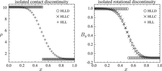
Figure 1.— Results for the isolated stationary contact (left) and rotational (right) discontinuities. Density and $B_{y}$ are shown, respectively. Plus signs, crosses, and open circles correspond to results with HLL, HLLC, and HLLD scheme, respectively. The number of grid points is $N_{x}=40$.

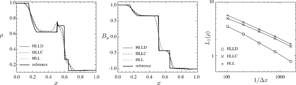
Figure 2.— Results for model MHDST1 at $t=0.4$. Density and $B_{y}$ are plotted in the left and central panels, respectively. Solid, dashed and dotted curves denote results of the first order HLLD, HLLC, and HLL schemes with $N_{x}=400$, while thick solid curves do those for the second order HLLD scheme with $N_{x}=6400$ (reference solution), respectively. A right panel shows the $L_{1}(\rho)$ norm compared with reference solutions. Open circles, crosses, and plus signs correspond to those for HLLD, HLLC, and HLL schemes, respectively.

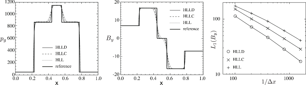
Figure 3.— Results for model MHDST2 at $t=0.4$. The gas pressure and $B_{y}$ profiles are plotted in the left and central panels, respectively. Solid, dashed and dotted curves denote results of the first order HLLD, HLLC, and HLL schemes with $N_{x}=400$, while thick solid curves do those for the second order HLLD scheme with $N_{x}=6400$ (reference solution), respectively. A right panel shows the $L_{1}(B_{y})$ norm compared with reference solutions. Open circles, crosses, and plus signs correspond to those for HLLD, HLLC, and HLL schemes, respectively.

4.1. Relativistic Ideal Magnetohydrodynamics

We perform four numerical tests of one-dimensional shock tube problems without radiation and resistivity. An initial discontinuity is situated at $x=0.5$ in a computational domain of $x=[0,1]$. Initial states of left ($x<0.5$) and right ($x>0.5$) regions for each problem are listed in Table 1.

In the following subsection, relativistic MHD equations are solved using a 1st order accurate scheme in space. Numerical fluxes are computed by HLL (Harten et al., 1983), HLLC (Mignone & Bodo, 2006), and HLLD (Mignone et al., 2009) scheme. We note that the results by the alternative HLLC scheme (Honkkila & Janhunen, 2007) are consistent with that by the scheme of Mignone & Bodo (2006).

An accuracy of our numerical code is verified by calculating $L-1$ norm:

$$L_{1}(g)=\sum_{i=1}^{N_{x}}|g^{ref}_{i}-g_{i}|\Delta x_{i},$$ (96)

where $N_{x}$ and $\Delta x_{i}$ are a number of grid points and a grid spacing. $g_{i}$ is a numerical solution of some physical quantities, while $g^{ref}_{i}$ is a reference solution. We use numerical results of a second order HLLD scheme with $N_{x}=6400$ for reference solutions, which are consistent with that with more grids. In this subsection, the CFL number is fixed to be 0.8.

4.1.1 Isolated contact and rotational discontinuities

For tests of stationary isolated contact and rotational discontinuities, which are proposed by Mignone et al. (2009), we employ $N_{x}=40$ and $\Gamma=5/3$. At the initial state, there is a density jump, while the other quantities are continuous for the isolated contact wave problem (see Contact Wave in Table 1). The velocity and magnetic field vectors are discontinuous, while $\rho$ and $p_{g}$ are invariant for the rotational discontinuity (see Rotational Wave in Table 1).

In Figure 1, we plot the density, $\rho$, for isolated contact discontinuity (left panel) and $y$-component of magnetic fields, $B_{y}$, for isolated rotational discontinuity (right panel) at $t=1.0$. Plus signs, crosses, and open circles denote results with HLL, HLLC, and HLLD solver, respectively.

We find in the left panel that HLLC and HLLD schemes, which intrinsically capture an entropy wave, can reproduce the contact surface, while a density profile becomes smoothed out in the case of HLL scheme. The right panel clearly shows that HLLD scheme, which can intrinsically capture the Alfvén wave, recovers a surface of the rotational discontinuity, in contrast to HLLC and HLL schemes. Here, we note that the profile of $B_{y}$ is slightly steeper by HLLC scheme than by HLL scheme at $x\sim 0.5$. This is because the numerical viscosity is smaller in HLLC scheme than in the HLL scheme. We recognize that our numerical code can capture the entropy wave by the HLLC and HLLD schemes, and Alfvén waves by HLLD scheme correctly.

4.1.2 MHD Shock Tube 1

The relativistic extension of the shock tube problem by Brio & Wu (1988) is proposed by many authors (Balsara, 2001; Del Zanna et al., 2003; Mignone & Bodo, 2006; Mignone et al., 2009). In this problem (model MHDST1), an initial discontinuity is broken up into a fast rarefaction wave, a compound wave, a contact discontinuity, a slow shock and a fast rarefaction wave, from left to right.

Figure 2 shows numerical results at $t=0.4$. Here, we employ $\Gamma=2$. Left and central panels show $\rho$ and $B_{y}$ profiles with $N_{x}=400$. Solid, dashed, and dotted curves denote results of 1st order HLLD, HLLC, and HLL schemes, while reference solutions are plotted by thick solid curves. Although the profile of the rarefaction wave front ($x\sim 0.1-0.3$) is almost independent of solvers, HLLD scheme only gives improved profiles at the compound wave ($x\simeq 0.5$), the contact surface ($x\simeq 0.6$), and the slow shock ($x\simeq 0.65$) (see also Fig. 3 in Mignone et al., 2009).

The right panel of Fig. 2 shows a $L_{1}$ norm of $\rho$ at $t=0.4$. We can see that the error linearly decreases with decreasing a grid size in all schemes. We note that HLLD scheme drastically reduces numerical errors compared to other solvers. We find $L_{1}^{\mathrm{HLL}}:L_{1}^{HLLC}:L_{1}^{HLLD}=1.0:0.91:0.55$, where superscripts of $L_{\rm 1}$ indicate the scheme. Here, note that the HLLD scheme takes a longer computational time. We find $t_{\mathrm{HLL}}:t_{\mathrm{HLLC}}:t_{\mathrm{HLLD}}=1:1.27:1.61$, where $t_{\mathrm{HLL}}$, $t_{\mathrm{HLLC}}$, and $t_{\mathrm{HLLD}}$ are computational time by HLL, HLLC, and HLLD scheme.

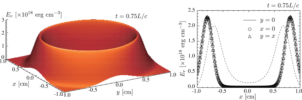
Figure 4.— (left) bird’s eye view of $E_{r}$ at $t=0.75L/c$. (right) 1-dimensional profiles of $E_{r}$ at $t=0.75L/c$. Solid curve denotes profiles on $y=0$, while open circles and open triangles denote $E_{r}$ on $x=0$ and $y=x$, respectively. Dashed curve also shows $E_{r}(x,y=0)$ but we initially set $F_{r}^{i}=0.$

4.1.3 MHD Shock Tube 2

We perform a test calculation for a collision of oppositely directing relativistic flows (model MHDST2, Balsara, 2001; Del Zanna et al., 2003; Mignone & Bodo, 2006; Mignone et al., 2009). Here, the bulk Lorentz factor is $\gamma\simeq 22.4$, and we set the specific heat ratio, $\Gamma$, to be $5/3$.

Figure  3 shows results at $t=0.4$. Left and central panels indicate profiles of $p_{g}$ and $B_{y}$. Solid, dashed, and dotted curves represent results of first order HLLD, HLLC, and HLL schemes with $N_{x}=400$, while a reference solution (a second order HLLD scheme with $N_{x}=6400$) is shown by thick solid curves.

We find in Figure  3 that two slow mode shocks ($x\sim 0.45$, $0.55$) are sandwiched by two fast mode shocks ($x\sim 0.2$, $0.8$) and that all of approximate Riemann solvers we adopted can capture the fastest mode (fast magnetosonic wave). Note that although a slow mode is not taken into account in HLLD scheme, less numerical viscosity leads to optimal solution.

The $L_{1}$ norm for $B_{y}$ is shown in the right panel of Figure 3. Filled circle, crosses, and plus signs indicate results with HLLD, HLLC, and HLL solver, respectively. The error linearly decreases with the grid spacing for all numerical schemes and the HLLD scheme is approved as the best numerical scheme in comparison with the other approximate Riemann solver. This panel also shows that the accuracy of HLLC scheme is better than that of HLL scheme (see also, Fig. 7 in Mignone et al., 2009). We find $L_{1}^{\mathrm{HLL}}:L_{1}^{HLLC}:L_{1}^{HLLD}=1.0:0.74:0.51$, and $t_{\mathrm{HLL}}:t_{\mathrm{HLLC}}:t_{\mathrm{HLLD}}=1:1.11:1.57$.

In addition to the problems mentioned above (Contact wave, Rotational wave, MHDST1, MHDST2), we performed several conventional one dimensional relativistic shock tube problems proposed by authors, and demonstrate the relativistic self-similar expansion of magnetic loop in two dimensions (Takahashi et al., 2011a). We confirmed that our numerical code can pass these problems.

4.2. Tests for Propagating Radiation Energy

We show results of numerical tests for propagating radiation energy. We recover a light speed $c$ in this subsection. Although we solve a full set of SR-RMHD equations throughout this subsection, the radiation hydrodynamics are not proofed. The propagation of radiation energy in the static fluid is virtually tested, since the radiation force as well as the gas pressure force is negligible and the velocity of the matter is almost kept null.

4.2.1 Point Explosion

We show an expansion of radiation field from a point source. We performed two-dimensional simulations in the $x-y$ plane with a volume bounded by $x=[-L,L]$ and $y=[-L,L]$, where $L=1~{}\mathrm{cm}$. We use uniformly spaced grids of $200\times 200$. We assume a static ($v=0$) and constant density profile with $\rho=1~{}\mathrm{g~{}cm^{-3}}$. The absorption coefficient is given by $\kappa=0.1~{}\mathrm{cm^{2}~{}g^{-1}}$, and the scattering coefficient is set to be null. Thus, a computational domain is optically thin, $\tau=\rho\kappa L=0.1$. The radiation energy and flux are initially given by

$$E_{r}=10^{10}E_{\mathrm{LTE}}\exp\left[-\frac{x^{2}+y^{2}}{0.01}\right],$$ (97)

$$F_{x}=cE_{r}\frac{x}{\sqrt{x^{2}+y^{2}}}$$ (98)

$$F_{y}=cE_{r}\frac{y}{\sqrt{x^{2}+y^{2}}},$$ (99)

where $E_{\mathrm{LTE}}=a_{R}T_{r}^{4}=10^{10}~{}\mathrm{erg~{}cm^{-3}}$ is the radiation energy density at the local thermodynamic equilibrium (LTE, $T_{g}=T_{r}$). Here $T_{r}$ is the radiation temperature. We solve the SR-RMHD equations with an first order accuracy in space and time.

A left panel of Figure 4 shows bird’s eye view of radiation energy density, $E_{r}$, at $t=0.75L/c$. Also, one-dimensional profiles of $E_{r}$ on $x$-axis (solid curve), $y$-axis (open circles), and $y=x$ (open triangles) are plotted in a right panel. Following initial enhancements of radiation energy, the radiation energy propagates in a circle with a light speed. Since most of the radiation energy is transported without absorption by matter, the radiation energy density decreases with a distance from the center, $r\equiv(x^{2}+y^{2})^{1/2}$, approximately as $E_{r}\propto r^{-1}$.

Such a caldera structure also appears even if we employ the Eddington approximation (Takahashi et al., 2013). However, in this method, the wave front propagates with a speed of $c/\sqrt{3}$. Such a reduction of the speed is induced by that the radiation field is assumed to be isotropic in Eddington approximation ($D_{r}^{ij}=1/3$). On the other hand, the Eddington tensor is given by taking account of the non-isotropic radiation fields in the M-1 closure (see Equations [17]-[20]). Turner & Stone (2001) attempted a similar test problem with using FLD approximation. They also succeeded in reproducing the propagating radiation energy with speed of light. However, since the radiation flux is basically given by the gradient of the radiation energy density in FLD, a caldera structure is not formed and the top-hat shaped distribution of the radiation energy density appears. The M-1 closure has an advantage when the radiation transport in an optically thin medium is considered.

The right panel of Figure 4 shows 1-dimensional profiles of $E_{r}$ at $t=0.75L/c$. A solid curve denotes profiles at $y=0$, while open circles and open triangles denote $E_{r}$ at $x=0$ and $y=x$, respectively. As discussed above, the radiation energy is transported with the light speed and a caldera structure is formed. We can see that these three profiles are consistent, indicating that the space symmetry is assured in our numerical code.

In this test problem, non-zero radiation fluxes are initially given by $|\mbox{\boldmath$F$}_{r}|=cE_{r}$. Then the radiation energy propagates radially with light speed. When we take $F^{i}_{r}=0$ initially, the radiation energy slowly expands compared to former results. This can be confirmed in the right panel of Figure 4. A dashed curve shows $E_{r}(x,y=0)$ at $t=0.75L/c$ for a model that $F_{r}^{i}$ is initially zero. We find that the wave front is slightly delayed for $|\mbox{\boldmath$F$}_{r}(t=0)|=0$ in comparison with that for $|\mbox{\boldmath$F$}_{r}(t=0)|=cE_{r}$. This is because that the Eddington tensor becomes $1/3$ when $|\mbox{\boldmath$F$}_{r}|=0$, leading to the wave velocity of $c/\sqrt{3}$. Since the expansion speed approaches to the light speed as time goes on, the gap of the wave fronts does not widen furthermore. Note that the characteristic wave velocity remains $c/\sqrt{3}$ around the origin via the nearly isotropic radiation fields. It makes profiles more diffusive. Hence, the radiation energy density for the case of $|\mbox{\boldmath$F$}_{r}(t=0)|$=0 is not null around the origin.

4.2.2 Beam

We show a radiation transport with a certain angle to a grid (Richling et al., 2001; González et al., 2007). We used $400\times 400$ grid points which cover the computational domain $x=[0,L]$ and $y=[0,L]$ where $L=1~{}\mathrm{cm}$. We assume a constant density profile of $\rho=1~{}\mathrm{g~{}cm^{-3}}$. We assume $\kappa=1~{}\mathrm{g\ cm^{-3}}$ and $\sigma_{s}=0$, leading the optical depth of $\tau=\rho\kappa L=1$. The radiation field is in LTE with a matter, whose energy is $E_{r}=E_{\mathrm{LTE}}=10^{10}~{}\mathrm{erg~{}cm^{-3}}$. We inject radiation from the boundary, $x=0$ and $y=[0.1,\ 0.2]$. The injected radiation energy is $E_{\mathrm{inj}}=10^{5}E_{\mathrm{LTE}}$ and the radiation flux is given by $F_{x}=F_{y}=cE_{r}/\sqrt{2}$. We adopted a free-boundary condition at the other boundaries. The SR-RMHD equations are solved with 2nd order accuracy in space and time.

Figure  5 shows a snapshot of $E_{r}$ at $t=2.0L/c$. We can see that a beam profile can be sharply captured in our numerical scheme thanks to a 2nd order accurate scheme. If we employ the Eddington approximation, the beam would broaden since the isotropic radiation field is assumed (this point will be discussed again in §4.2.3). Also, the beam can not be reproduced in principle in the case of FLD approximation. Since the radiation flux is given as a function of the the gradient of $E_{r}$, the radiation energy propagates in a circle.

We plot in Figure 6 that the radiation energy density along the beam ($y=x+0.15$) at $t=0.5,1.0,2.0L/c$. Here $l$ is a distance from the center of the injection point [$(x,\ y)=(0,\ 0.15)$]. The radiation front, which propagates with a speed of light, can be excellently captured thanks to the 2nd order accurate scheme.

Since the radiation energy is absorbed by the matter, and since the emission of the matter is negligible, the radiation energy density decreases with an increase of $l$. Then, the profile of $E_{r}$ is analytically expressed as

$$E_{r}(l)=E_{\mathrm{inj}}\exp(-\rho\kappa l),$$ (100)

within the wave front of $l=ct$ (a dashed curve). We can see that our numerical results excellently recover the analytical solution.

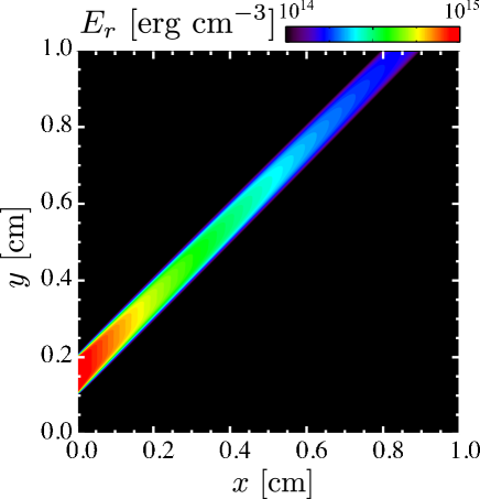
Figure 5.— Snapshot of $E_{r}$ at $t=2L/c$ for the beam test.

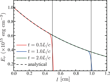
Figure 6.— Profiles of the radiation energy along the beam at $t=0.5L/c$ (red), $1.0L/c$ (blue) and $2.0L/c$ (green). Thin solid curves denote the wave front at $t=0.5L/c$ and $t=L/c$, while a black dashed curve represents an analytical solution of steady model.

4.2.3 Shadow

We show the light propagation around a dense matter. This test was proposed by Hayes & Norman (2003) and González et al. (2007) adopted the M-1 formulation to the problem. We perform simulations with M-1 closure and with Eddington approximation.

We utilize a simulation box bounded by $x=[-5,10]~{}\mathrm{km}$ and $y=[0,5]~{}\mathrm{km}$ with grid points of $300\times 100$. By setting $C_{\mathrm{cfl}}=0.5$, the timestep is $\Delta t=C_{\mathrm{CFL}}\Delta x/c=8.3\times 10^{-8}\mathrm{s}$. We set $\sigma_{s}=0$ in the whole range of the domain. We consider a dense clump embedded in the less dense matter. The clump is located at the origin. The radius and the mass density are $r_{0}=2~{}\mathrm{km}$ and $\rho_{1}=30~{}\mathrm{g~{}cm^{-3}}$. The density of the surrounding rarefied matter is set to be $\rho_{0}=10^{-6}~{}\mathrm{g~{}cm^{-3}}$. Since we here suppose $\kappa=10^{-2}~{}\mathrm{cm^{2}}~{}g^{-1}$, the optical thickness of the clump is $\rho_{1}\kappa r_{0}=6\times 10^{4}$, and the less dense region is optically thin, $\rho_{1}\kappa\times 15{\rm km}=0.015$. The radiation energy density is set to be constant, $E_{r}=E_{\mathrm{LTE}}=10^{5}~{}\mathrm{erg~{}cm^{-3}}$, and the rarefied matter is LTE, initially. We assume a uniform gas temperature with $T_{g}=T_{r}$ at the initial state.

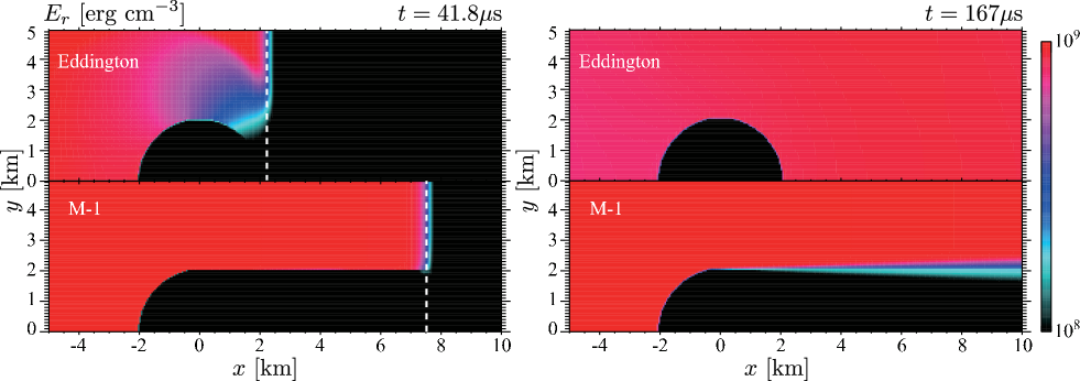
Figure 7.— Color contours of $E_{r}$ at $t=41.8\mu s$ and $167\mu s$ for a shadow test. White dashed lines in the left panel show wave fronts at $x=-0.5\ \mathrm{cm}+ct/\sqrt{3}$ with the Eddington approximation and $x=-0.5\ \mathrm{cm}+ct$ with the M-1 closure.

The radiation is injected at the left boundary, $x=-5~{}\mathrm{km}$, where the radiation energy density, $E_{\mathrm{inj}}$, is set to be $10^{4}E_{\mathrm{LTE}}$, and the radiation flux is assumed as $F^{x}_{r}=cE_{r}$ with M-1 closure and $F^{x}_{r}=cE_{r}/\sqrt{3}$ with Eddington approximation. A free boundary condition is employed at the upper ($x=10~{}\mathrm{km}$) and right ($y=5~{}\mathrm{km}$) boundaries. At $y=0$, we use a symmetric boundary.

The radiation energy density at $t=41.8~{}\mathrm{\mu s}$ (left) and $167~{}\mathrm{\mu s}$ (right), which correspond to $0.83$ and $3.3$ light crossing time along the $x$-direction, is presented by color contours in Figure 7. Upper and lower panels are results with Eddington and M-1 methods, respectively. In this Figure, we can see a shadow behind the clump in M-1 method ($x>2.0$ km). Since the parallel light injected from the left boundary is absorbed by the dense clump, and since the photons are not scattered ($\sigma_{s}=0$), the lower right region of $x>2.0$ km and $y<2.0$ km is darkened by shadow. Here, we note that HLL scheme is better than simple Lax-Friedrich scheme in order to reproduce such a sharp discontinuity (González et al., 2007). In contrast with M-1 method, the shadow does not appear in the case of Eddington model. As we have mentioned, since the isotropic radiation fields are assumed, the radiation comes around behind the clump even without scattering.

Figure 7 also shows that the radiation energy propagates with speed of light for M-1 model. The dashed line in the left lower panel indicates a wave front computed from $x=-0.5\ \mathrm{cm}+ct$. The resulting wave front is in good agreement with the dash line. On the other hand, a wave speed reduces to $c/\sqrt{3}$ in the Eddington model as we have discussed above. In the upper left panel, we find that the position of a wave front is $x\sim 2.2$ km, which is consistent with the estimation of $x=-0.5\ \mathrm{cm}+ct/\sqrt{3}$ with $t=41.8~{}\mathrm{\mu s}$.

We stress here again about the advantage of implicit treatment for gas-radiation interaction (source terms). In this problem, the timescale of the gas-radiation interaction, $(\rho_{1}\kappa c)^{-1}$, is around $1.1\times 10^{-10}\ \mathrm{s}$ in the clump, which is much shorter than the timestep, $8.3\times 10^{-8}\mathrm{s}$. If we explicitly integrate the gas-radiation interaction terms, the numerical instability is caused. We can take longer timestep via the implicit treatment.

4.3. Tests for radiation hydrodynamics

In this subsection, we show the qualitative difference between the M-1 closure scheme and the Eddington approximation by solving the shock tube problems proposed by Farris et al. (2008). Although they obtained semi-analytic solutions by assuming the Eddington approximation, there are no analytic solutions with the M-1 closure due to the non-linearity in the Eddington tensor. Since our numerical code can recover their analytical solutions by adopting Eddington approximation in place of the M-1 closure (Takahashi et al., 2013), we clearly understand the feature of the M-1 closure scheme and difference from the Eddington approximation.

A simulation box is bounded by $x=[-L,L]$, where $L=20$ in the normalized unit. A number of grid points is fixed with $N_{x}=3200$ in this subsection. Unlike Farris et al. (2008), initially the discontinuity is situated at $x=0$. The gas and radiation are in local thermal equilibrium in both sides ($x>0$ and $x<0$). The free boundary condition is applied in both boundaries ($x=-L$ and $x=L$). We again take the light speed as unity. The Stefan-Boltzmann constant has a fictitious value of $a_{R}=E^{\prime}_{r,L}/T^{4}_{g,L}$, which is used to evaluate $E^{\prime}_{r,R}=a_{r}T_{g,R}^{4}$ (Farris et al., 2008; Zanotti et al., 2011), where the dash denotes a quantity defined in the comoving frame, and subscripts $L$ and $R$ denote the left ($x<0$) and right ($x>0$) states, respectively. A parameter set of initial conditions is summarized in Table 1.

4.3.1 non-relativistic strong shock

Figure 8 shows the result of a non-relativistic strong shock problem (model RHDST1). We plot the mass density, gas temperature, radiation energy density and radiation flux measured in the comoving frame, and the ratio of $F_{r}^{\prime}$ to $E_{r}^{\prime}$ at $t=5000$ from top to bottom. Solid curves denote solutions of M-1 model, while dashed curves represent numerical solutions of the Eddington model.

Since the radiation energy density is much less than the gas energy density, and since the radiation force does not play an important role, the mass density and the gas temperature have a sharp discontinuity at the shock $(x=0)$ like a shock tube problem with pure hydrodynamics. We also find that there is fewer differences between two models as for the profiles of $\rho$ and $T_{g}$. In contrast, the profiles of $E^{\prime}_{r}$ and $F^{\prime x}_{r}$ by M-1 model are slightly different for those by Eddington model. The radiation energy is transported from the shock front ($x=0$) to the pre-shocked region ($x<0$) in both models. The radiation flux is approximately given as $-E^{\prime}_{r}$ for the M-1 model and as $-E^{\prime}_{r}/\sqrt{3}$ for the Eddington model (note that the speed of light is set to be unity in this subsection), so that the ratio of $F^{\prime x}_{r}$ to $E^{\prime}_{r}$ is smaller at $x\leq 0$ for the M-1 model than for the Eddington model (bottom panel). In addition, the radiation field is attenuated at the precursor region via the absorption in both models. However, we find that the gradient of the profiles of $E^{\prime}_{r}$ and $F^{\prime x}_{r}$ are smoother in the M-1 model than in the Eddington model (see the region of $x<0$). The radiation field reduces with a distance from the shock front, $\propto e^{-\rho\kappa|x|}$, for the M-1 model, but $\propto e^{-\sqrt{3}\rho\kappa|x|}$, for the Eddington model. Such a difference is induced by that the propagating speed of the radiation is decreased as $1/\sqrt{3}$ in the Eddington model as we have discussed above.

4.3.2 relativistic shock

A second shock tube problem is a relativistic shock including a radiation (model RHDST2). Here, four velocity in the upstream is taken to be 10. Figure 9 shows profiles of mass density, temperatures of gas (thick curves) and radiation (thin curves), radiation energy density, flux and $xx$-component of the Eddington tensor at $t=5000$ from top to bottom. Solid and dashed curves denote for solutions with the M-1 closure and the Eddington approximation. In this test, the shock front is stationary for the Eddington model, but it very slowly moves with a speed of $1.6\times 10^{-4}$ for the M-1 model. In this figure, the position of shock front is readjusted so as to be located at the origin in order to compare solutions between two models.

We can see that solutions (except for $D^{\prime xx}$) between two models are qualitatively and quantitatively consistent. This is because that the optical depth is large enough, and, then, the Eddington approximation is valid. However, we find that $D_{r}^{\prime xx}$ slightly deviates from $1/3$ for the M-1 model, although $D_{r}^{\prime xx}$ is $1/3$ by definition for the Eddington model. The radiation energy is transported from the shock front to the precursor region, leading to the slight anisotropic radiation field. In our M-1 model, the maximum of $F^{\prime x}_{r}/E_{r}^{\prime}$ is $\simeq 0.31$ and then we find $D_{r}^{\prime xx}=0.38$.

Here, we note that the gas temperature is higher than the radiation temperature in the preshocked region, although the gas temperature could not exceed the radiation temperature, $T_{g}\leq T_{r}$, if the gas is mainly heated up by absorption. We confirmed that the compression is the dominant heating mechanism.

Figure 8.— 1-dimensional plots of the mass density, gas temperature, radiation energy density measured in the comoving frame, radiative flux measured in the comoving frame, and $F_{r}^{\prime x}/E_{r}^{\prime}$

for the non-relativistic strong shock. Solid and dashed curves denote results with the M-1 closure and the Eddington approximation, respectively.

4.3.3 radiation pressure dominated shock

In a radiation dominated mildly relativistic shock problem (model RHDST3), the upstream radiation energy density is set to be 20 times larger than the gas internal energy, although the ratio is $2.2\times 10^{-4}$ and $3.3\times 10^{-2}$ for tests in §4.3.1 and §4.3.2, respectively.

Figure 10 shows profiles of $\rho,v^{x},E^{\prime}_{r},F^{\prime x}_{r}$, and forces acting on a gas at $t=5000$ from top to bottom. In upper four panels, solid and dashed curves denote solutions of M-1 and Eddington models. In the bottom panel, solid and dotted curves represent the radiation gas pressure gradient force for the M-1 model, respectively. After an initial discontinuity at $x=0$ breaks up, a steady state solution, in which the shock front is located at the origin, gradually forms in the Eddington model. In the case of the M-1 model, although the shock moves with a constant velocity of $v_{sh}=-5.3\times 10^{-4}$, the profiles approach to a steady solution for the frame of reference in which the shock front is stationary. Similar to two tests have shown in §4.3.1 and §4.3.2, a precursor wave propagates in a upstream region.

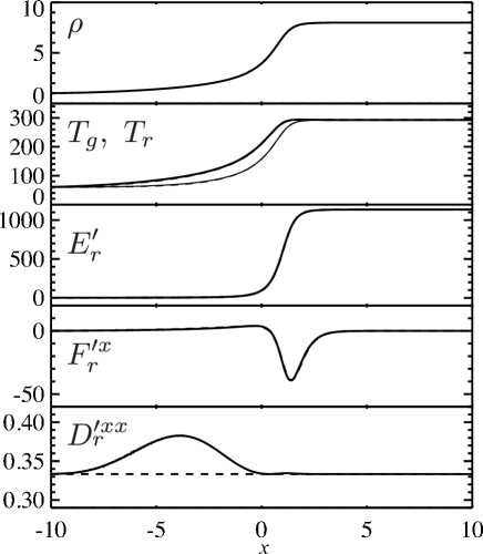
Figure 9.— 1-dimensional profiles of the relativistic shock. From the top to bottom panels, the mass density, gas (thick curve) and radiation (thin curve) temperatures, radiation energy density, radiation flux, and $xx$-component of the Eddington tensor, are plotted, These quantities are measured in the comoving frame. Solid and dashed curves respectively shows the results with M-1 and Eddington models.

Figure 10.— 1-dimensional plot of the mass density, $v^{x}$, radiation energy density measured in the comoving frame, radiation flux measured in the comoving frame, and forces acting on the plasma for the radiation shock. In the top four panels, solid and dashed curves denote the results with the M-1 closure and the Eddington approximation, respectively. In the bottom panel, the solid and dotted curves denote the radiative force and the gas pressure gradient force.

It is found that the radiation flux is negative in both models (forth panel), implying that the radiation energy is transported from right to left. The leftward radiation flux ($-F^{\prime x}_{r}$), which is at maximum at around $x=0$ (M-1) or $x=-3$ (Eddington), is reduced by absorption and approaches to null with decreasing $x$. Although the radiation energy is transported up to merely $x\sim-7$ for Eddington model, the leftward radiation penetrates to $x\sim-12$ for M-1 model. Since the speed of light is effectively reduced to $1/\sqrt{3}$ as we have discussed above, the leftward radiation flux suddenly decreases via the enhanced absorption for the Eddington model. Therefore, in the M-1 model, the profile of the radiation energy density is smooth, the radiation energy density is enhanced even at the range of $x<-7$.

The leftward radiation flux in the upstream region induces the leftward radiation force (bottom panel), which works to decrease the velocity. Hence, the velocity (density) starts to decrease (increase) at $x\sim-12$ for M-1 model and $x\sim-7$ for Eddington model (see top and second panels). The bottom panel clearly shows that the pressure gradient force is weaker than the radiation force. Here we note that, in contrast with RHDST1, the precursor strongly affects on the upstream gas since a radiation energy much exceeds a gas energy density in the present test.

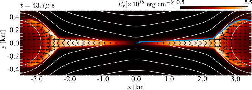
Figure 11.— Color shows $E_{r}$ at $t=47.3\ \mu\mathrm{s}$, while white curves and arrows denote for magnetic field lines and radiation flux, respectively. A blue line denotes a position at which there is a steep jump on $j_{z}$ in the first quadrant.

4.4. Relativistic Petschek Type Magnetic Reconnection with Radiation Field

Lastly, we perform a SR-R2MHD simulation of a relativistic magnetic reconnection. Recently, some authors have studied the relativistic magnetic reconnection without radiation by assuming uniform resistivity model (Takahashi et al., 2011b) and a spatially localized resistivity model (Watanabe & Yokoyama, 2006; Zenitani et al., 2010; Zanotti & Dumbser, 2011). Also the importance of the radiative effects on the magnetic reconnection is studied (Steinolfson & van Hoven, 1984; Jaroschek & Hoshino, 2009; Uzdensky & McKinney, 2011). In this section, we adopt a spatially localized resistivity model for a fast (Petschek type) magnetic reconnection.

We solve SR-R2MHD equations in the Cartesian coordinate on the $x-y$ plane. A computational domain consist of $x=[0,\ 17.4]\ \mathrm{km}$ and $y=[0,\ 5.7]\ \mathrm{km}$. We use non uniform grids and a number of grid points is $(N_{x},N_{y})=(3500,\ 800)$. A minimum grid size is $\Delta x=\Delta y=100\mathrm{cm}$. Because of the symmetry of the system, we adopt a point symmetric boundary condition. Scalar quantities are symmetric at $x=0$ and $y=0$. At $x=0$, $u^{y},B^{x},B^{z},E^{x},E^{z},F_{r}^{y}$ are symmetric while the rest of the vector components are anti-symmetric. At $y=0$, $u^{x},B^{y},B^{z},E^{y},E^{z},F_{r}^{x}$ are symmetric and the vector components are anti-symmetric. The free boundary conditions are applied at the other boundaries. We assume an isothermal and uniform gas, $\rho_{0}=0.01~{}\mathrm{g~{}cm^{-3}}$ and $T_{g}=10^{8}~{}\mathrm{K}$ in a whole domain at the initial state. The gas is initially in LTE, $T_{g}=T_{r}$. We assume a force free magnetic field configuration given by

$$\mbox{\boldmath$B$}=B_{0}\tanh\left(\frac{y}{\lambda}\right)\mbox{\boldmath$e$}_{x}+B_{0}\mathrm{sech}\left(\frac{y}{\lambda}\right)\mbox{\boldmath$e$}_{y},$$ (101)

(Low, 1973; Komissarov et al., 2007), where $B_{0}=10^{10}~{}\mathrm{G}$ is an amplitude of the magnetic field and $\mbox{\boldmath$e$}_{x}$ and $\mbox{\boldmath$e$}_{y}$ are unit vectors in $x$- and $y$-direction. $\lambda=10^{4}~{}\mathrm{cm}$ is a thickness of a current sheet. Since we take a mean molecular weight to be $0.5$, the plasma-$\beta$ in initial state is $4.1\times 10^{-5}$.

We adopt a spatially localized resistivity model to attain the fast magnetic reconnection:

$$\eta=\eta_{u}+\frac{\eta_{i}-\eta_{u}}{\cosh[(x^{2}+y^{2})/\lambda]^{2}},$$ (102)

where $\eta_{u}$ and $\eta_{i}$ are constants. We set corresponding magnetic Reynolds numbers as $R_{M,u}=4\pi\lambda c/\eta_{u}=400$ and $R_{M,i}=4\pi\lambda c/\eta_{i}=50$. For opacity, we assume electron scattering and free-free absorption. The typical optical depth is $40$ for scattering and $6.4\times 10^{-6}$ for absorption.

Figure 11 shows results at $t=47.3\mu\mathrm{s}$. Color, arrows, and white curves indicate the radiation energy density, flux, and magnetic field lines in the observer frame. A blue line denotes a position at which there is a steep jump on $j_{z}$ in the first quadrant.

Due to an enhancement of the electric resistivity at the origin, magnetic field lines start to reconnect and the gas is evacuated as outflows in the $\pm x$-directions. Since we adopt a spatially localized resistivity model, four slow shocks attached to the diffusion region form (one of them is indicated by a blue curve) (Watanabe & Yokoyama, 2006; Zenitani et al., 2010; Zanotti & Dumbser, 2011). This indicates that a fast Petschek type magnetic reconnection is realized even though the radiation field is fulfilled.

We can see that the radiation energy density is confined in exhausts of outflows. The photons suffer from numerous scattering, since the system is very optically thick for scattering. Thus, the radiation flows together with matter via advection, and $\mbox{\boldmath$F$}_{r}$ is almost parallel to velocity fields. This implies that the reconnection region is very brightly observed for downstream observers (on $x$-axis). On the other hand, it would be difficult to detect the reconnection region for observers around $y$-axis or $z$-axis.

In order to consider radiation effects on the dynamics, we plot in Figure 12 the pressure gradient force including effects of enthalpy variation (blue), electromagnetic force with non-adiabatic term (red), radiation force (orange), and total force density (black) along a slow shock denoted by a blue line in Figure 11. This figure clearly shows that the electromagnetic force accelerates the gas and the pressure gradient force is negligible. The matter is decelerated by the radiation force. Such a deceleration is caused by the radiation drag ($\propto(v^{i}E_{r}+v_{j}P_{r}^{ij}$) which becomes non-negligible compared with the radiation flux force ($\propto F_{r}$), when $F^{i}_{r}<(v^{i}E_{r}+v_{j}P_{r}^{ij})$. In the present problem, the condition of $F^{i}_{r}<(v^{i}E_{r}+v_{j}P_{r}^{ij})$ is moderately realised since the large optical thickness reduces the radiation flux. The typical value of $F^{x}_{r}/(v^{x}E_{r}+v_{j}P_{r}^{xj})$ is around unity.

In the present problem, the radiation drag is also non-negligible compared with the electromagnetic force. Here, we recover a light speed $c$ to avoid misunderstanding. The ratio of the radiation drag to the electromagnetic force is $\rho\sigma_{s}vE_{r}l/4\pi c\mbox{\boldmath$B$}^{2}$, where we assume a mildly relativistic plasma and estimate the radiation drag and the electromagnetic force as $\sim\rho\sigma_{s}vE_{r}/c$ and $\sim 4\pi\mbox{\boldmath$B$}^{2}/l$ with $l$ being a typical length of the current sheet for the order estimation. Such a ratio is rewritten as $0.5\tau_{\mathrm{cs}}(E_{r}/E_{\rm mag})(v/c)$, where $E_{\mathrm{mag}}(=\mbox{\boldmath$B$}^{2}/8\pi)$ is the magnetic energy density and $\tau_{\mathrm{cs}}(=\rho l\sigma_{s})$ is the optical depth of the current sheet. It implies that the radiation drag tends to play an important role for magnetic reconnection in the high density and high velocity plasma. In our simulations, we have $\tau_{\mathrm{cs}}(E_{r}/E_{\rm mag})(v/c)\sim 3.6$ by assuming $l=\lambda$ and $v=v_{A}=B/\sqrt{4\pi\rho}$. Due to the radiation drag, the outflow four velocity is about 10% slower with the radiation field than without the radiation field in our parameter set.

In Figure 13, we show a time evolution of reconnection rate, which is here defined by $E_{z}(0,0)/B_{0}$ ($x$- and $y$-components of the electric fields are null by definition). Solid and dashed curves are results with and without solving radiation field, respectively. Due to an enhancement of the localized resistivity, magnetic field lines start to reconnect and amplitude of electric field rapidly increases by dissipating the magnetic energy. After $t=30\ \mu\mathrm{s}$, quasi steady state is realized and the reconnection rate roughly becomes constant. The reconnection rate at the steady state is about 10% smaller with the radiation field than without the radiation field. It is understood as below. As we have already mentioned, the radiation drag force slows down the outflow velocity. Then, the inflow velocity in the quasi steady state (downward and upward component of the velocity in the regions of $y>0$ and $y<0$) is also reduced. Thus, the $z$-component of the electric fields, [$E_{z}=-(\mbox{\boldmath$v$}\times\mbox{\boldmath$B$})_{z}/c$], decreases, inducing the reduction of the magnetic reconnection rate.

Although we show the results for one parameter set, the reconnection rate as well as the outflow velocity, would depend on initial parameters. The systematic study of the magnetic reconnection with radiation fields will be reported in the forthcoming paper.

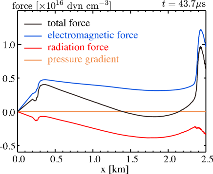
Figure 12.— Total (black), electromagnetic (blue), radiation (red) and pressure gradient (orange) force densities acting on the fluids along the slow shock.

Figure 13.— Time evolution of the reconnection rate $E_{z}(0,0)/B_{0}$. Solid and dashed curves denote for results with and without radiation fields, respectively.

5. Summary

We developed a special relativistic radiation-magnetohydrodynamic (SR-RMHD) code, in which the M-1 closure method is employed and a source term for gas-radiation interaction is implicitly and iteratively integrated. We also extend our SR-RMHD code to a special relativistic resistive radiation-MHD (SR-R2MHD) code, which includes electric resistivity. Our SR-RMHD code successfully solves some of test problems, i.e., shock tube problems of MHD/Radiation-HD and propagating radiation, and we demonstrate the radiation drag effect in relativistic Petschek type magnetic reconnection by SR-R2MHD code.

Since our code use radiation fields only in the observer’s frame, we straightforwardly compute $\mbox{\boldmath$P$}_{r}$ from $E_{r}$ and $\mbox{\boldmath$F$}_{r}$ through the M-1 closure method without the Lorentz transformation. In contrast, the Lorentz transformation is inevitable for the Eddington approximation. By virtue of M-1 closure method, anisotropic propagation of radiation is solved and the propagating speed of the radiation is $c$ in the optically thin media. The Eddington approximation as well as flux-limited diffusion approximation is problematic for such anisotropy. In addition, the speed of light is reduced to be $c/\sqrt{3}$ for the Eddington approximation.

In our code, all of advection terms are explicitly integrated by setting the timestep to be a fraction of $\Delta x/c$ with $\Delta x$ being the grid spacing. Implicit integration of the source term prevents the timestep from shortening when the timescale of the source term (e.g., gas-radiation interaction) becomes very small. For the implicit treatment, we directly invert a $4\times 4$ matrix at each grid point in SR-RMHD code. In addition to the gas-radiation interaction term, the source term appeared in Ampere’s law is also solved implicitly in SR-R2MHD code. Then, we need to invert $3\times 3$ and $4\times 4$ matrices at each grid point. Such matrix inversion is carried out analytically without communication with neighbor grids. Thus, our code could be massively parallelized without difficulty. Our code would be widely utilized for the relativistic astrophysical phenomena, even though the dense and less dense regions are mixed.

References

- Balbus & Hawley (1991) Balbus, S. A. & Hawley, J. F. 1991, ApJ, 376, 214
- Balsara (2001) Balsara, D. 2001, ApJS, 132, 83
- Blackman & Field (1993) Blackman, E. G. & Field, G. B. 1993, Physical Review Letters, 71, 3481
- Blandford & Payne (1982) Blandford, R. D. & Payne, D. G. 1982, MNRAS, 199, 883
- Brio & Wu (1988) Brio, M. & Wu, C. C. 1988, Journal of Computational Physics, 75, 400
- Chandrasekhar (1960) Chandrasekhar, S. 1960, Proceedings of the National Academy of Science, 46, 253
- Colella & Woodward (1984) Colella, P. & Woodward, P. R. 1984, Journal of Computational Physics, 54, 174
- Dedner et al. (2002) Dedner, A., Kemm, F., Kröner, D., Munz, C., Schnitzer, T., & Wesenberg, M. 2002, Journal of Computational Physics, 175, 645
- Del Zanna & Bucciantini (2002) Del Zanna, L. & Bucciantini, N. 2002, A&A, 390, 1177
- Del Zanna et al. (2003) Del Zanna, L., Bucciantini, N., & Londrillo, P. 2003, A&A, 400, 397
- Eggum et al. (1987) Eggum, G. E., Coroniti, F. V., & Katz, J. I. 1987, ApJ, 323, 634
- Eggum et al. (1988) —. 1988, ApJ, 330, 142
- Farris et al. (2008) Farris, B. D., Li, T. K., Liu, Y. T., & Shapiro, S. L. 2008, Phys. Rev. D, 78, 024023
- Fromang et al. (2012) Fromang, S., Latter, H. N., Lesur, G., & Ogilvie, G. I. 2012, ArXiv e-prints
- Fromang et al. (2007) Fromang, S., Papaloizou, J., Lesur, G., & Heinemann, T. 2007, A&A, 476, 1123
- González et al. (2007) González, M., Audit, E., & Huynh, P. 2007, A&A, 464, 429
- Harten et al. (1983) Harten, A., Lax, P. D., & van Leer, B. 1983, SIAM Rev., 25, 35
- Hayes & Norman (2003) Hayes, J. C. & Norman, M. L. 2003, ApJS, 147, 197
- Hirose et al. (2009) Hirose, S., Blaes, O., & Krolik, J. H. 2009, ApJ, 704, 781
- Honkkila & Janhunen (2007) Honkkila, V. & Janhunen, P. 2007, Journal of Computational Physics, 223, 643
- Icke (1980) Icke, V. 1980, AJ, 85, 329
- Icke (1989) —. 1989, A&A, 216, 294
- Jaroschek & Hoshino (2009) Jaroschek, C. H. & Hoshino, M. 2009, Physical Review Letters, 103, 075002
- Jiang et al. (2013) Jiang, Y.-F., Stone, J. M., & Davis, S. W. 2013, ApJ, 767, 148
- Kato et al. (2008) Kato, S., Fukue, J., & Mineshige, S. 2008, Black-Hole Accretion Disks — Towards a New Paradigm —, ed. Kato, S., Fukue, J., & Mineshige, S.
- Komissarov (1999) Komissarov, S. S. 1999, MNRAS, 308, 1069
- Komissarov (2007) —. 2007, MNRAS, 382, 995
- Komissarov et al. (2007) Komissarov, S. S., Barkov, M., & Lyutikov, M. 2007, MNRAS, 374, 415
- Kudoh & Shibata (1997) Kudoh, T. & Shibata, K. 1997, ApJ, 476, 632
- Lesur & Longaretti (2007) Lesur, G. & Longaretti, P.-Y. 2007, MNRAS, 378, 1471
- Levermore (1984) Levermore, C. D. 1984, J. Quant. Spec. Radiat. Transf., 31, 149
- Low (1973) Low, B. C. 1973, ApJ, 181, 209
- Lynden-Bell (1978) Lynden-Bell, D. 1978, Phys. Scr, 17, 185
- Machida et al. (2006) Machida, M., Nakamura, K. E., & Matsumoto, R. 2006, PASJ, 58, 193
- Martí & Mueller (1996) Martí, J. & Mueller, E. 1996, Journal of Computational Physics, 123, 1
- McKinney & Blandford (2009) McKinney, J. C. & Blandford, R. D. 2009, MNRAS, 394, L126
- Mignone & Bodo (2006) Mignone, A. & Bodo, G. 2006, MNRAS, 368, 1040
- Mignone & McKinney (2007) Mignone, A. & McKinney, J. C. 2007, MNRAS, 378, 1118
- Mignone et al. (2009) Mignone, A., Ugliano, M., & Bodo, G. 2009, MNRAS, 393, 1141
- Minerbo (1978) Minerbo, G. N. 1978, J. Quant. Spec. Radiat. Transf., 20, 541
- Ohsuga (2006) Ohsuga, K. 2006, ApJ, 640, 923
- Ohsuga & Mineshige (2011) Ohsuga, K. & Mineshige, S. 2011, ApJ, 736, 2
- Ohsuga et al. (2009) Ohsuga, K., Mineshige, S., Mori, M., & Kato, Y. 2009, PASJ, 61, L7+
- Ohsuga et al. (2005) Ohsuga, K., Mori, M., Nakamoto, T., & Mineshige, S. 2005, ApJ, 628, 368
- Okuda & Fujita (2000) Okuda, T. & Fujita, M. 2000, PASJ, 52, L5
- Palenzuela et al. (2009) Palenzuela, C., Lehner, L., Reula, O., & Rezzolla, L. 2009, MNRAS, 394, 1727
- Richling et al. (2001) Richling, S., Meinköhn, E., Kryzhevoi, N., & Kanschat, G. 2001, A&A, 380, 776
- Roedig et al. (2012) Roedig, C., Zanotti, O., & Alic, D. 2012, MNRAS, 426, 1613
- Sa̧dowski et al. (2013) Sa̧dowski, A., Narayan, R., Tchekhovskoy, A., & Zhu, Y. 2013, MNRAS, 429, 3533
- Shibata et al. (2011) Shibata, M., Kiuchi, K., Sekiguchi, Y., & Suwa, Y. 2011, Progress of Theoretical Physics, 125, 1255
- Simon & Hawley (2009) Simon, J. B. & Hawley, J. F. 2009, ApJ, 707, 833
- Steinolfson & van Hoven (1984) Steinolfson, R. S. & van Hoven, G. 1984, ApJ, 276, 391
- Stone et al. (1992) Stone, J. M., Mihalas, D., & Norman, M. L. 1992, ApJS, 80, 819
- Tajima & Fukue (1996) Tajima, Y. & Fukue, J. 1996, PASJ, 48, 529
- Takahashi et al. (2011a) Takahashi, H. R., Asano, E., & Matsumoto, R. 2011a, MNRAS, 414, 2069
- Takahashi et al. (2011b) Takahashi, H. R., Kudoh, T., Masada, Y., & Matsumoto, J. 2011b, ApJ, 739, L53
- Takahashi et al. (2013) Takahashi, H. R., Ohsuga, K., Sekiguchi, Y., Inoue, T., & Tomida, K. 2013, ApJ, 764, 122
- Takamoto & Inoue (2011) Takamoto, M. & Inoue, T. 2011, ApJ, 735, 113
- Takeuchi et al. (2010) Takeuchi, S., Ohsuga, K., & Mineshige, S. 2010, PASJ, 62, L43+
- Tchekhovskoy et al. (2010) Tchekhovskoy, A., Narayan, R., & McKinney, J. C. 2010, ApJ, 711, 50
- Turner & Stone (2001) Turner, N. J. & Stone, J. M. 2001, ApJS, 135, 95
- Uchida & Shibata (1985) Uchida, Y. & Shibata, K. 1985, PASJ, 37, 515
- Uzdensky & McKinney (2011) Uzdensky, D. A. & McKinney, J. C. 2011, Physics of Plasmas, 18, 042105
- van Leer (1977) van Leer, B. 1977, Journal of Computational Physics, 23, 263
- Velikhov (1959) Velikhov, E. P. 1959, Soviet Physics JETP, 36, 995
- Watanabe & Yokoyama (2006) Watanabe, N. & Yokoyama, T. 2006, ApJ, 647, L123
- Zanotti & Dumbser (2011) Zanotti, O. & Dumbser, M. 2011, MNRAS, 418, 1004
- Zanotti et al. (2011) Zanotti, O., Roedig, C., Rezzolla, L., & Del Zanna, L. 2011, MNRAS, 417, 2899
- Zenitani et al. (2009) Zenitani, S., Hesse, M., & Klimas, A. 2009, ApJ, 696, 1385
- Zenitani et al. (2010) —. 2010, ApJ, 716, L214