Physical characteristics of G331.5-0.1:
The luminous central region of a Giant Molecular Cloud

Abstract

We report molecular line and dust continuum observations toward the high-mass star forming region G331.5-0.1, one of the most luminous regions of massive star-formation in the Milky Way, located at the tangent region of the Norma spiral arm, at a distance of 7.5 kpc. Molecular emission was mapped toward the G331.5-0.1 GMC in the CO$(J=1\rightarrow$0) and C¹⁸O$(J=1\rightarrow$0) lines with NANTEN, while its central region was mapped in CS($J=2\rightarrow 1$ and $J=5\rightarrow 4$) with SEST, and in CS$(J=7\rightarrow$6) and ¹³CO$(J=3\rightarrow$2) with ASTE. Continuum emission mapped at 1.2 mm with SIMBA and at 0.87 mm with LABOCA reveal the presence of six compact and luminous dust clumps, making this source one of the most densely populated central regions of a GMC in the Galaxy. The dust clumps are associated with molecular gas and they have the following average properties: size of 1.6 pc, mass of $3.2\times 10^{3}$ $\mathrm{M}_{\sun}$, molecular hydrogen density of $3.7\times 10^{4}$ cm^-3, dust temperature of 32 K, and integrated luminosity of $5.7\times 10^{5}$ $\mathrm{L}_{\sun}$, consistent with values found toward other massive star forming dust clumps. The CS and ¹³CO spectra show the presence of two velocity components: a high-velocity component at $\sim-89$ km s^-1, seen toward four of the clumps, and a low-velocity component at $\sim-101$ km s^-1 seen toward the other two clumps. Radio continuum emission is present toward four of the molecular clumps, with spectral index estimated for two of them of 0.8$\pm$0.2 and 1.2$\pm$0.2. A high-velocity molecular outflow is found at the center of the brightest clump, with a line width of 26 km s^-1 (FWHM) in CS$(J=7\rightarrow$6) . Observations of SiO($J=7\rightarrow 6$ and $J=8\rightarrow 7$), and SO($J_{K}=8_{8}\rightarrow 7_{7}$ and $J_{K}=8_{7}\rightarrow 7_{6}$) lines provide estimates of the gas rotational temperature toward this outflow $>$120 K and $>75$ K, respectively.

I. Introduction

Massive stars play a key role in the evolution of the Galaxy; hence they are important objects of study in astrophysics. Although their number is much smaller than the low mass stars, they are the principal source of heavy elements and UV radiation, affecting the process of formation of stars and planets (Bally et al., 2005) and the physical, chemical and morphological structure of galaxies (e.g. Kennicutt, 1998, 2005).

Diverse studies show that massive stars are formed in the denser regions of giant molecular clouds (GMC) (Churchwell et al., 1990; Cesaroni et al., 1991; Plume et al., 1992; Bronfman et al., 1996). The formation process of high-mass stars is, however, still under debate (Garay & Lizano, 1999). Observationally, recently formed massive stars cannot be detected at optical wavelengths because they are embedded within regions with high dust extinction. Another problem arises from theoretical considerations: a star with a mass larger than eight solar masses starts burning hydrogen during the accretion phase and the radiation pressure may halt or even reverse the infall process (e.g. Larson & Starrfield, 1971; Kahn, 1974; Yorke & Kruegel, 1977; Wolfire & Cassinelli, 1987; Edgar & Clarke, 2004; Kuiper et al., 2010). Due to these difficulties, a paradigm that explains the formation of massive stars does not exist (Zinnecker & Yorke, 2007; McKee & Ostriker, 2007), contrary to the successful model accepted for low mass stars. Understanding the physical process that dominates during the early stages of the formation of massive stars and its influence back on its harboring molecular gas requires a study of the physical conditions of the environment previous to the star formation or at very early stages.

The object of our study is one of the most massive GMCs in the Southern Galaxy, at $l=331.5\arcdeg$ and $b=-0.1$, in the tangent region of the Norma spiral arm (Bronfman et al., 1985, 1989). Several observations have shown that the central region of this GMC harbors one of the most extended and luminous regions of massive star formation in the Galactic disk. Single dish radio continuum observations show the presence of an extended region of ionized gas (G331.5$-$0.1), with an angular size of $\sim 3\arcmin-4$′(projected size 6.5-8.7 pc at a distance of 7.5 kpc), close to the peak CO position of the GMC (Shaver & Goss, 1970; Caswell & Haynes, 1987). From observations of the H109$\alpha$ and H110$\alpha$ hydrogen recombination lines, Caswell & Haynes (1987) determined that the line central velocity of the ionized gas is $\sim$ -89 km s^-1, similar to the peak velocity of the GMC. The dynamical timescale of the region of ionized gas is $\sim 8.5\times 10^{5}$ years, and the rate of ionizing photons required to excite the H II region is $1.1\times 10^{50}$ s^-1. In addition, IRAS observations show the presence of an extended source, with an angular size similar to that of the ionized region and a FIR luminosity of 3.6$\times 10^{6}$ $\mathrm{L}_{\sun}$.

While both the ionizing photon rate and the FIR luminosity could be provided by a single O4 ZAMS star, it is most likely that the ionization and the heating of the region is provided by a cluster of massive OB stars. This explanation is supported by Midcourse Space Experiment and Spitzer Space Telescope-GLIMPSE survey data, which show that there are several sites of massive star formation spread over a region of $\sim 6^{\prime}$ in diameter. Bronfman et al. (2000) showed that toward the $l=331\arcdeg$ galactic longitude, there is a peak in the number density of IRAS sources with colors of ultracompact H II (UCHII) regions and associated with CS$(2\rightarrow$1) emission, which are thought to correspond to massive star forming regions.

Evidence of active star formation in the G331.5$-$0.1 GMC is further provided by the detection of OH and methanol maser emission (Goss et al., 1970; Caswell et al., 1980; Caswell, 1997, 1998; Pestalozzi et al., 2005), as well as H₂O maser emission (Caswell, private communication). Hydroxyl masers are known to be excellent indicators of UCHII regions, whereas methanol maser emission is a common phenomenon in regions of massive star formation (Menten et al., 1986) and H₂O maser emission is thought to be a probe of the earliest stages of massive star formation (Furuya, 2003). Also, within a radius of 4.5’ centered on the peak position of G331.5$-$0.1 there are three objects from the Red MSX Source (RMS) catalog of Massive Young Stellar Objects (MYSOs) candidates (Urquhart et al., 2008), further indicating that the G331.5$-$0.1 central region is an active region of massive star formation. In addition, Bronfman et al. (2008) showed the presence of a compact, extremely high velocity molecular outflow in the G331.5$-$0.1 region, suggesting that it is driven by one of the most luminous and massive objects presently known. The G331.5$-$0.1 region is thus an ideal region to study extremely active massive star formation in GMCs.

Here we present observations and a thorough analysis of the G331.5$-$0.1 region with dust continuum and molecular line emission data. Section 2 describes the telescopes used and methods of data acquisition. Section 3 describes the results of our study at several scales, starting from GMCs ($\sim$100 pc), to molecular clumps sizes ($\sim$1 pc) and reaching sub-parsec scales in our interferometric data. This analysis considers dust emission and different molecular line tracers, along with mid-infrared and far-infrared data from SPITZER, MSX and IRAS telescopes, and free-free emission at cm wavelengths. Section 4 describes the physical parameters derived from our observations, including mass, density and bolometric luminosity estimates. We also include a rotational temperature analysis for a massive and energetic molecular outflow in the G331.5$-$0.1 GMC central region. Our results are summarized in section 5.

II. Observations

We observed emission in several molecular lines and continuum bands using several telescopes located in northern Chile: the NANTEN telescope of Nagoya University at the Las Campanas observatory, the 15-m Swedish-ESO Submillimetre Telescope (SEST) at La Silla, the 10-m Atacama Submillimeter Telescope Experiment (ASTE) at Pampa la Bola, and the 12-m Atacama Pathfinder Experiment (APEX) located in Llano Chajnantor. We also made observations using the Australia Telescope Compact Array (ATCA) located at Narrabri, Australia. The basic parameters of the molecular line observations are summarized in Table 1. Column 1 gives the telescope used, Col. 2 and 3, the observed transition and line frequency, respectively. Col. 4 and 5 the half-power beam width and the main beam efficiency. Col. 6 to 10 give, respectively, the number of positions observed, the angular spacing, the integration time on source per position, the channel width and the resulting rms noise in antenna temperature, for each of the observed transitions. The observing parameters for the continuum observations are summarized in Table 2.

II.1. NANTEN Telescope

The NANTEN telescope is a 4-m diameter millimeter telescope designed for a large-scale survey of molecular clouds. With this telescope we observed the emission in the CO$(J=1\rightarrow$0) ($\nu=115271.202$ MHz) and C¹⁸O$(J=1\rightarrow$0) ($\nu=109782.173$ MHz) lines during several epochs between 1999 and 2003. The half-power beam width of the telescope at 115 GHz is 2.6′, providing a spatial resolution of 5.7 pc at the assumed distance of the source of 7.5 kpc. The observed maps consisted in grids of 585 positions for the CO emission and 440 positions for the C¹⁸O emission, with spacing between observed positions of 2.5′ (nearly the beam size of the instrument at the observed frequencies). The front-end was a superconductor-isolator-superconductor (SIS) receiver cooled down to 4 K with a closed-cycle helium gas refrigerator, and the backend was an acousto-optical spectrometer (AOS) with 2048 channels. The total bandwidth was 250 MHz and the frequency resolution was 250 kHz, corresponding to a velocity resolution of $\sim$ 0.15 km s^-1. The typical system noise temperature was $\sim$ 250 K (SSB) at 115 GHz and $\sim$ 160 K (SSB) at 110 GHz. The main beam efficiency of the telescope is 0.89. A detailed description of the telescope and its instruments are given by Ogawa et al. (1990), Fukui et al. (1991) and Fukui & Sakakibara (1992). Data reduction were made using the NANTEN Data Reduction Software (NDRS).

II.2. Swedish-ESO Submillimetre Telescope (SEST)

II.2.1 Millimeter continuum

The 1.2 mm continuum observations were carried out using the 37-channel hexagonal Sest IMaging Bolometer Array (SIMBA) during 2001. The passband of the bolometer has an equivalent width of 90 GHz and is centered at 250 GHz (1200 $\mu$m). At the frequency band of SIMBA, the telescope has an effective beamwidth of 24″ (FWHM), that provides a spatial resolution of 0.87 pc at a distance of 7.5 kpc. The rms noise achieved is $\sim$50 mJy/beam. Data reduction was made using the package MOPSI (Mapping On-Off Pointing Skydip Infrared). The maps were calibrated from observations of Mars and Uranus and the calibration uncertainties are estimated to be lower than 20%.

II.2.2 Molecular lines

With SEST we observed the emission in the CS$(J=5\rightarrow$4) ($\nu$ = 244935.644 MHz) and CS$(J=2\rightarrow$1) ($\nu$ = 97980.968 MHz) lines during May 2001. The half-power beam width and the main beam efficiency of the telescope were 22″ and 0.48 at 245 GHz, and 52″ and 0.73 at 98 GHz, respectively. The total bandwidth was 43 MHz and the frequency resolution was 43 kHz, corresponding to a velocity resolution of $\sim$ 0.05 km s^-1 for the CS$(5\rightarrow$4) observations, and a velocity resolution of $\sim$ 0.13 km s^-1 for the CS$(2\rightarrow$1) observations. The typical system noise temperature was 350 K for CS$(5\rightarrow$4) observations and 250 K for CS$(2\rightarrow$1) observations. The CLASS (Continuum and Line Analysis Single-dish Software) software, part of the GILDAS package, was used for data reduction.

Figures A1 and A2 on the online material present maps of the observed spectra toward the G331.5$-$0.1 central region in the CS$(2\rightarrow$1) and CS$(5\rightarrow$4) line emission over 81 positions with a spacing of 45″. The CS$(2\rightarrow$1) map then is well sampled, while the CS$(5\rightarrow$4) map is undersampled at this spacing, considering the smaller beam size at that frequency.

II.3. Atacama Submillimeter Telescope Experiment

With ASTE we observed the emission in the CS$(J=7\rightarrow$6) ($\nu$ = 342882.950 MHz) and ¹³CO$(J=3\rightarrow$2) ($\nu$ = 330587.957 MHz) lines during 2005 July and 2006 July. ASTE has a beam size at 350 GHz of 22″ (FWHM). For both transitions 167 positions were sampled, within a $\sim 360\arcsec\times 360\arcsec$ region with 22.5″ spacing in position-switched mode, with the OFF position located at $\alpha_{2000}=16^{h}14^{m}08.4^{s}$ and $\delta_{2000}=-51\arcdeg 37\arcmin 23\arcsec$. The system temperatures ranged between 179 and 233 K, resulting in a rms noise antenna temperature of typically 0.1 K for an integration time of 4 minutes.

Main-beam temperatures, $T_{MB}=T^{*}_{A}/\eta_{MB}$, obtained by dividing the antenna temperature $T^{*}_{A}$ by the main-beam efficiency, $\eta_{MB}$, are used throughout the analysis. During the first part of the observations, we mapped a grid of 88 positions, with $\eta_{MB}=0.65$. On July, 2006. we completed the map observing 79 new positions, with $\eta_{MB}=0.77$. The 1024 channels of the 350 GHz band receiver provided a bandwidth of 128 MHz, and a channel width of 0.125 MHz. The data reduction was carried out by use of the AIPS-based software package NEWSTAR developed at NRO.

Figures A3 and A4 on the online material present maps of the observed spectra toward the G331.5$-$0.1 central region in the CS$(7\rightarrow$6) and ¹³CO$(3\rightarrow$2) line emission over 167 positions with a spacing of 22.5″ (similar to the beam size of the instrument at this frequency).

II.4. Atacama Pathfinder Experiment

II.4.1 Millimeter continuum: the ATLASGAL survey

The millimeter observations of the region were made as part of the APEX Telescope Large Area Survey of the Galaxy (ATLASGAL) project, which is a collaboration between the Max Planck Gesellschaft (MPG: Max Planck Institute für Radioastronomie, MPIfR Bonn, and Max Planck Institute für Astronomie, MPIA Heidelberg), the European Southern Observatory (ESO) and the Universidad de Chile. ATLASGAL is an unbiased survey of the inner region of the Galactic disk at 0.87 mm, made using the 295-channel hexagonal array Large Apex BOlometer CAmera (LABOCA), that operates in the 345 GHz atmospheric window, with a bandwidth of about 60 GHz. The angular resolution is 18.6″ (HPBW) (corresponding to a resolution of 0.68 pc at a distance of 7.5 kpc) and the total field of view is 11.4′. The survey covers an area of $\pm$1.5° in galactic latitude, and $\pm$60° in longitude, with a sensitivity of 50 mJy/beam (Schuller et al., 2009).

II.4.2 Molecular lines

Using the APEX-2a heterodyne receiver, we observed the emission in the SiO$(J=7\rightarrow$6) ($\nu$ = 303926.809 MHz), SiO$(J=8\rightarrow$7) ($\nu$ = 347330.635 MHz), SO$(8_{7}\rightarrow 7_{6}$) ($\nu$ = 304077.844 MHz) and SO$(8_{8}\rightarrow 7_{7}$) ($\nu$ = 344310.612 MHz) lines during May 2007. The telescope has a beam size of 17.5″ at 345 GHz, corresponding to a spatial resolution of 0.63 pc at a distance of 7.5 kpc. The main beam efficiency of the telescope is $\eta_{MB}=0.73$ and the system temperature was $\sim$ 170 K. The observations were made toward the peak position of the CO$(7\rightarrow$6) outflow emission ($\alpha_{2000}=16^{h}12^{m}10.09^{s}$ and $\delta_{2000}=-51\arcdeg 28\arcmin 38.4\arcsec$) reported by Bronfman et al. (2008). The data were reduced using the CLASS software of the GILDAS package.

II.5. Australia Telescope Compact Array

The ATCA radio continuum observations were made in two epochs: 2002 November using the 6A configuration and 2005 November using the 1.5C configuration. These configurations utilize all six antennas and cover east-west baselines from 0.5 to 6 km. Observations were made at the frequencies of 4.80 and 8.64 GHz (6 and 3.6 cm), with a bandwidth of 128 MHz. The FWHM primary beam of ATCA at 4.8 GHz and 8.6 GHz are, respectively, 10′ and 6′. The total integration time in each frequency was 2.5 hr.

The calibrator PKS 1600-48 was observed before and after every on-source scan in order to correct the amplitude and phase of the interferometer data due to atmospheric and instrumental effects. The flux density was calibrated by observing PKS 1934-638 (3C84) for which values of 5.83 Jy at 4.8 GHz and 2.84 Jy at 8.6 GHz were adopted. Standard calibration and data reduction were performed using MIRIAD (Sault et al., 1995). Maps were made by Fourier transformation of the uniformly weighted interferometer data using the AIPS task IMAGR. The noise level in the 4.8 and 8.6 GHz images are, respectively, 0.41 and 0.37 mJy beam^-1. The resulting synthesized (FWHM) beams are $2.7\arcsec\times 1.8\arcsec$ at 4.8 GHz and $1.5\arcsec\times 1.0\arcsec$ at 8.6 GHz.

III. Results

III.1. The G331.5$-$0.1 Giant Molecular Cloud

Figure 1 shows grey scale maps and contours of the velocity integrated CO and C¹⁸O emission between 330.9° $<$ l $<$ 332.3° and -0.42° $<$ b $<$ 0.14°. The range of the velocity integration is from -117.7 to -73.2 km s^-1, chosen from the average spectrum of the region (shown in Fig. 2). The contours represent 20% to 90%, in steps of 10%, of the peak intensity of each map (297.6 K km s^-1 for CO, 19.6 K km s^-1 for C¹⁸O). The rms noise of the CO and C¹⁸O maps are 19.8 K km s^-1 and 0.98 K km s^-1, respectively. The emission at 50% of the peak is shown with a thicker contour in each map. The CO emission arises from an extended cloud elongated along the galactic longitude, with major and minor axes of 81.7′ and 18.9′ (full width at half-power), which imply linear sizes of 178 by 41 pc at the assumed distance of 7.5 kpc. The peak position on the CO map is located at $l=331.5\arcdeg,\ b=-0.125\arcdeg$, with an intensity of 297.6 K km s^-1.

To estimate the kinematic distance of the G331.5$-$0.1 cloud, we locate it in the subcentral point at the source longitude, for the following reasons. Using the Galactic rotation curve derived by Alvarez et al. (1990), with Ro = 8.5 kpc and Vo = 220 km s^-1, and a mean average velocity of -92.8 km s^-1 for the integrated GMC spectrum, the near kinematic distance would be 5.7 kpc and the far kinematic distance 9.2 kpc. While the near distance has been preferred by Goss et al. (1972), the far distance has been considered by Kerr & Knapp (1970). However, the GMC has two velocity components, at -100 km s^-1 and -90 km s^-1 (see section III.2.2), the lowest one almost reaching the terminal velocity due to pure rotation of -110 km s^-1. Caswell & Haynes (1987) reported hydrogen recombination line absorption at $l=331.515\arcdeg,b=-0.069$, with a $V_{LSR}$ of -89 km s^-1, as well as H₂CO absorption lines at -99.8 and -89.3 km s^-1, favoring the far distance, even when they adopted the near distance following Goss et al. (1972). Nevertheless, Bronfman et al. (1996) reported emission in CS$(2\rightarrow$1) from the IRAS point source 16086-5119, at $l=331.552,b=-0.115$, with a $V_{LSR}$ of -100.7, corresponding to the higher velocity component, so the continuum source for the H₂CO absorption lines at both velocities is most probably the IRAS point source at -100 km s^-1, setting them both at the near distance.

Given the large spread in velocity of the integrated spectrum; the presence of two velocity components for the GMC, the lowest one almost reaching the terminal velocity; and the conflicting evidence for locating the GMC at the far or near distance, we will consider in the estimation of its physical parameters that the G331.5$-$0.1 cloud is located in the tangent of the Norma spiral arm, at a distance of $\sim$7.5 kpc, corresponding to the subcentral point. With this assumption, the distance of the GMC will have an estimated uncertainty of $\sim$ 30$\%$, given by the near and far kinematic positions, leading to an uncertainty in the estimation of masses and luminosities of a factor of $\sim$2. A recent study of kinematic distances using HI absorption done by Jones & Dickey (2012) puts the region G331.552-0.078, located toward the peak position of our CO emission maps, at the Norma spiral arm tangent point distance, at 7.47 kpc, a similar value to the one used in the present work.

The emission in the C¹⁸O$(1\rightarrow$0) line has a position angle of approximately $\sim$30° with respect to the galactic longitude, with observed major and minor axes of 18.2′ and 11.6′, respectively (39.7 $\times$ 25.3 pc at a distance of 7.5 kpc). The size of the C¹⁸O structure is four times smaller than the CO cloud. It is necessary to keep in mind that the appearance and dimension of a molecular cloud depend strongly on the tracer used to observe it (Myers, 1995). The CO observations most likely trace all the gas within the GMC, including low and high column density gas, while C¹⁸O is tracing only the high column density gas. The C¹⁸O peak position coincides with the peak emission in the CO$(1\rightarrow$0) line. Fitting gaussian profiles to the spectra observed at $l$=331.5°, $b$=-0.125°, we determine $V_{lsr}=-89.7$ km s^-1 and $\Delta V$ (FWHM) = 3.8 km s^-1 for CO, and $V_{lsr}=-89$ km s^-1 and $\Delta V$ (FWHM) = 2.9 km s^-1 for the C¹⁸O emission.

Using the C¹⁸O$(1\rightarrow$0) integrated map, we define the central region of the G331.5$-$0.1 GMC as the region that emits more than seventy percent of the peak integrated emission (red dashed box in Figure 1). This area is 7′ in size ($\sim$15 pc at the source distance) and it is centered at $l$ = 331.523°, $b$ = -0.099° ($\alpha_{2000}=16^{h}12^{m}12^{s}$ and $\delta_{2000}=-51\arcdeg 28\arcmin 00\arcsec$). The central region is a single structure coherent in velocity, as it can be seen on the position-velocity maps for CO and C¹⁸O (Fig. 3). Further observations with better angular resolution have shown that this region has two velocity components, with a difference of $\sim$12 km s^-1 (see section III.2.2).

Figure 4 shows a map of the emission observed at 870 $\mu$m by ATLASGAL between 331° $<$ l $<$ 332° and -0.4° $<$ b $<$ 0.15°. Overlaid is a velocity integrated C¹⁸O emission map. The range of velocity integration and the emission contours are the same as for Figure 1. The 0.87 mm map also shows the position of 13 sources (two of them are double sources) from the RMS catalog in the proximity of the tangent area of the Norma spiral arm. Clearly there is a concentration of dust continuum emission sources towards the defined central region of the cloud (red dashed box in Figure 4). Six millimeter-wave compact sources were identified inside the defined G331.5$-$0.1 GMC central region, and three of them are associated to RMS sources. This suggests an active formation of massive stars within the central region of G331.5$-$0.1 GMC.

III.2. The G331.5$-$0.1 GMC central region

In this section we present a detailed study of millimeter continuum and molecular line observation toward the 7′$\times$7′ area defined in the previous section as the G331.5$-$0.1 GMC central region. The beam sizes of the observations ($\sim$30″) are approximately five times better than the observations of CO$(1\rightarrow$0) and C¹⁸O$(1\rightarrow$0), and they give information in the $\sim$1 pc at a distance of 7.5 kpc. The maps of G331.5$-$0.1 GMC have been presented so far in galactic coordinates, mainly to show the extension of this region in galactic longitude. Nevertheless, we present our observations here and following sections in a more traditional style using equatorial coordinates.

III.2.1 Dust emission: Millimeter continuum observations

Figure 5 presents maps of the 1.2 mm and 0.87 mm dust continuum emission observed with the SEST and APEX telescopes respectively. They reveal the presence of six dust continuum substructures with strong emission. We labeled these sources as MM1, MM2, MM3, MM4, MM5 and MM6, according to increasing order in right ascension. The observed parameters of the millimeter sources are given in Table 3. Column 3 and 4 give their peak position. Column 5 and 6 give the peak flux density and the total flux density, respectively, the latter measured with the AIPS task IMEAN. Column 7 give the deconvolved major and minor FWHM angular sizes obtained from Gaussian fits to the observed spatial distribution. Column 8 gives the physical size of the sources, obtained from the geometric mean of the angular size obtained at 1.2 mm and 0.87 mm, and considering a distance to the sources of 7.5 kpc. The average size of the millimeter sources within the G331.5$-$0.1 central region is 1.6 pc. Following the description of Williams et al. (2000), we refer to these millimeter-wave structures as clumps.

III.2.2 Molecular line emission

The observed parameters of the line emission detected at the peak position of the millimeter clumps are given in Table 4. Also given are the parameters of an average spectrum of each clump for the CS$(7\rightarrow$6) and ¹³CO$(3\rightarrow$2) lines, obtained from a three by three map centered at the peak position of each clump. For non-gaussian profiles, the velocity spread $\Delta V$ is estimated from $\Delta V\ =\ I(T_{A}^{*})\,/\,T^{*}_{A}\,{}_{Peak}$. The equations for $I(T_{A}^{*})$ and its associated error $\sigma^{2}_{I(T_{A}^{*})}$ are obtained from (e.g. Shirley et al., 2003)

$$I(T_{A}^{*}) = \int_{v_{1}}^{v_{2}}{T_{A}^{*}\,dv}$$

$$\sigma^{2}_{I(T_{A}^{*})} = \langle\sqrt{\Delta v_{line}\delta v_{chan}}\ \sigma_{T_{A}^{*}}\rangle^{2}_{map}+\sigma_{base}^{2}\ ,$$ (1)

with $\Delta v_{line}=v_{2}-v_{1}$ is the full velocity range of the line emission, $\delta v_{chan}$ is the velocity resolution of the spectrometer, and $\sigma_{T_{A}^{*}}$ is the uncertainty in the antenna temperature. The additional error contribution $\sigma_{base}$, from residual variation in the baseline due to linear baseline subtraction, was not considered. The error $\sigma_{I(T_{A}^{*})}$ was propagated into the uncertainty in $\Delta V$.

Figure 6 shows the spectra toward the peak intensity position of the clumps MM1 through MM6 in the molecular lines CS$(2\rightarrow$1), CS$(5\rightarrow$4), CS$(7\rightarrow$6) and ¹³CO$(3\rightarrow$2).

We discovered in the CS$(7\rightarrow$6) map the presence of a broad and strong wing emission toward the peak position of the brightest 1.2 mm clump (MM3), at $\alpha_{2000}=16^{h}12^{m}10.13^{s}$ and $\delta_{2000}=-51\arcdeg 28\arcmin 37.5\arcsec$. The characteristics of this spectrum, along with other CO emission lines, were previously reported by Bronfman et al. (2008). Their analysis indicates that it corresponds to an unresolved, energetic and massive molecular outflow (flow mass of $\sim 55\ \mbox{$\mathrm{M}_{\sun}$}$; momentum of $\sim 2.4\times 10^{3}\ \mbox{$\mathrm{M}_{\sun}$}$ km s^-1; kinetic energy of $\sim 1.4\times 10^{48}$ ergs).

The molecular transitions SiO$(7\rightarrow$6), SiO$(8\rightarrow$7), SO$(8_{7}\rightarrow 7_{6}$) and SO$(8_{8}\rightarrow 7_{7}$) were observed toward the position of the molecular outflow. SO and SiO trace shocked gas towards dense cores (see Gottlieb et al. 1978; Rydbeck et al. 1980; Swade 1989; Miettinen et al. 2006) where the density is high enough to excite it. High-velocity SiO and SO has been observed in some of the most powerful molecular outflows (e.g. Welch et al. 1981; Plambeck et al. 1982; Martin-Pintado et al. 1992), and our current understanding is that SiO and SO are evaporated from the dust grains when the shock velocity is greater than about 20 km s^-1, depending on the composition of the grain-mantle in the preshock gas (e.g. Schilke et al. 1997). Figure 7 shows the spectra of the SO and SiO lines.

Line profiles of the CS and CO emission show the presence of two distinct velocity components centered at $\sim-88.9$ and $\sim-100.8$ km s^-1 (see Fig. 6). Maps of the velocity integrated emission in the ranges of -93.9 to -84.4 km s^-1 and -105.4 to -95 km s^-1 are presented in Figures 8 and 9. Clumps MM1 and MM6 are associated with the lowest velocity component ($\sim-100.8$ km s^-1), while clumps MM2, MM3, MM4 and MM5 are associated with the high velocity component ($\sim-88.9$ km s^-1). There is a good correspondence between CS$(7\rightarrow$6) map and the dust continuum emissions (see Fig. 10), indicating that these two tracers are probes of regions with similar physical conditions. We will refer to the region including the four high-velocity clumps as the “complex of clumps” in the G331.5$-$0.1 GMC central region.

The angular sizes of the structures defined by the integration of the CS$(7\rightarrow$6) line and associated to the clumps, and the nominal radii resulting from the deconvolution of the telescope beam size, are summarized in Table 5. For MM3, the CS$(7\rightarrow$6) peak position and average spectra are well fitted with two gaussian components. The first component corresponds to the broad wind emission, associated with the high-velocity molecular outflow, while the second gaussian component corresponds to the ambient gas emission. For the peak position spectrum, the gaussian fit of the wing emission has $T_{A}^{*}=0.92\pm 0.12$ K and $\Delta v=31.1\pm 2.8$ km s^-1 (FWHM), and the ambient gas gaussian fitting has $T_{A}^{*}=1.40\pm 0.12$ K and $\Delta v=6.1\pm 0.1$ km s^-1 (FWHM).

III.2.3 Mid-infrared and far-infrared emission

Infrared observations are a useful tool to study the process of massive star formation. At these wavelengths, radiation is less affected by extinction than at visible wavelengths; therefore infrared observations can give us information of the nearby environment of newly formed massive stars that are surrounded and obscured by cool dust. The mid-infrared (range 5 - 25 $\mu$m) and far-infrared (range 25 - 400 $\mu$m) observations are dominated by the thermal emission from dust, that re-radiates the absorbed UV radiation from newly born OB stars and reprocessed photons from the ionized nebula. In the mid-infrared range the contribution from polycyclic aromatic hydrocarbons, from which emission is strong in photo-dissociation regions, is also significant.

Figure 11 shows a three color infrared image made using data from the IRAC bands at 3.6 $\mu$m (blue), 4.5 $\mu$m (green) and 8.0 $\mu$m (red), overlaid with contours of the emission at 0.87 mm. While the infrared emission agrees with the millimeter emission in the global sense, the 8.0 $\mu$m emission seems to trace the envelope of a ionized region, with the millimeter emission of the complex of clumps, surrounding this structure. Also, we find strong and compact emission associated with the MM3 clump in the three IRAC bands, with an angular size of $\sim 14\arcsec$.

For each millimeter clump, we measured the integrated flux densities in the four Spitzer IRAC bands (8.0 $\mu$m, 5.8 $\mu$m, 4.5 $\mu$m and 3.6 $\mu$m, Fazio et al. 2004), on the MSX bands (21.3 $\mu$m, 14.7 $\mu$m, 12.1 $\mu$m and 8.3 $\mu$m, Mill et al. 1994) and IRAC bands (100 $\mu$m, 60 $\mu$m, 25 $\mu$m and 12 $\mu$m, Neugebauer et al. 1984). The results are tabulated in Table 6.

III.3. High angular resolution observations of the G331.5$-$0.1 GMC central region.

We present in this section interferometric observations of radio continuum emission toward the G331.5$-$0.1 GMC central region. The beam size of the observations ($\sim$2″) allow us to study compact structures at sub-parsec scales. The analysis also considered association between the radio continuum components found in recent OH and methanol maser catalogs at high resolution.

III.3.1 Radio continuum emission

Figure 12 shows contour maps of the radio continuum emission at 6 and 3.6 cm towards the central region of G331.5$-$0.1 GMC. Our observations reveal the presence of four distinct compact radio sources within the mapped field of 10′, labeled as components A,B,C and D, and associated with the clumps MM1, MM4, MM3 and MM6, respectively (see Fig. 11). The positions, flux densities and beam deconvolved sizes (FWHM) of the sources, obtained with the AIPS task IMFIT, are given in Table 7.

Components A, B and D are also associated, respectively, with the G331.4904-00.1173, G331.5414-00.0675, and G331.5582-00.1206 RMS sources candidates to MYSOs (Urquhart et al., 2008). The detection of radio emission indicate that these three candidates are UCHII regions and therefore related with a more evolved state than a genuine MYSOs. The brightest radio source (component C) is associated with the very energetic outflow detected towards the G331.5$-$0.1 central region (Bronfman et al., 2008). Figure 13 shows the radio spectra of all four components. Components B and C exhibit an increasing flux density with frequency, thus they could be optically thick ultracompact regions or stellar wind sources. The dotted line corresponds to the best fit of the spectral energy distribution (SED) assuming that they correspond to regions of ionized gas with uniform density, and that the emission can be modeled as a modified blackbody, with $I_{\nu}=B_{\nu}(T_{e})[1-\exp(-\tau_{\nu})]$ and the opacity $\tau$ estimated from (Wilson et al., 2009):

$$\tau_{\nu}=8.235\times 10^{-2}\left(\frac{T_{e}}{\mathrm{K}}\right)^{-1.35}\left(\frac{\nu}{\mathrm{GHz}}\right)^{-2.1}\left(\frac{EM}{\mathrm{pc\ cm^{-6}}}\right)\ ,$$ (2)

with $T_{e}$ the electron temperature and $EM$ the emission measure. We considered $T_{e}=10^{4}$ K. The derived spectral indexes of component B and C are given in Column 9 of Table 7. Component B has a spectral index of the radio emission between 4.8 and 8.6 GHz of 0.8$\pm$0.2, similar the value expected for a spherical, isothermal, constant-velocity model of stellar wind (Reynolds, 1986). The error in the determination of spectral indexes include the 5% uncertainty in the absolute flux density scale. Component C spectral index has a value of 1.2$\pm$0.2 already reported by Bronfman et al. (2008). This index suggests that source C corresponds to an ionized jet which is likely to drive the associated energetic molecular outflow.

Components A and D are more extended than B and C, and they present a decrease in the integrated flux density from 4.8 to 8.6 GHz. We attribute this particular behavior to an observational artifact, that could be related with a less complete uv-coverage at higher frequency. An estimation of the flux density inside an area comparable with the beam size ($\sim$2.5″) gives an almost flat spectrum for component A, and even though the flux still decreases with frequency for component D, the flux difference was reduced from 47% to 30%. We expected for both sources, A and D, a flat spectral energy distribution in the radio continuum, consistent with the free-free emission from a thermal source.

III.3.2 Maser emission

Earlier studies of masers across our Galaxy have shown that regions of high-mass star formation can be associated with OH, H₂O and Class II methanol masers (Caswell et al., 1995; Szymczak et al., 2002). In particular, OH masers are usually considered signposts of UCHII regions, while methanol masers are found associated to hot molecular cores, UCHII regions and near-IR sources (Garay & Lizano, 1999; Bartkiewicz & van Langevelde, 2012). Therefore, OH and methanol masers often coincide, and they are found in regions with active star formation. With this in mind, we searched in methanol and OH surveys toward the Norma spiral arm region. We found three sources from the 6-GHz methanol multibeam maser catalog from Caswell et al. (2011). Two of them, 331.542-0.066 and 331.543-0.066, are toward the MM4 millimeter clump and they are coincident, within the errors, with the radio component B. The velocity of the peak reported for these maser sources are -86 km s^-1 and -84 km s^-1 respectively, within 5 km s^-1 difference from the molecular line velocities of MM4 shown in Table 4, and therefore consistent with the ambient velocity of the complex of clumps. The third 6668 MHz methanol maser spot, 331.556-0.121 ($\alpha_{2000}=16^{h}12^{m}27.21^{s}$ and $\delta_{2000}=-51\arcdeg 27\arcmin 38.2\arcsec$), is associated with the MM6 millimeter clump, it has a velocity at peak emission of -97 km s^-1, similar to values found with molecular lines for MM6, and it is located 5.8″ ($\sim$3 times the beamsize in the maser catalog) away from the peak position of radio component D. Each of these three maser spots has a counterpart OH maser (Caswell, 2009, 1998). The peak position of radio component C ($\alpha_{2000}=16^{h}12^{m}10.04^{s}$, $\delta_{2000}=-51\arcdeg 28\arcmin 37.7\arcsec$) is coincident, within the errors, with the interferometrically derived position of an 1665 MHz OH maser spot (G331.512-0.103; Caswell, 1998). No methanol class II emission was reported towards the outflow up to a detection limit of 0.6 Jy (Caswell et al., 2011). The position of masers in the G331.5$-$0.1 GMC central region is shown in Fig. 12, along their association with the radio continuum sources.

No methanol or OH emission is associated with the MM1, MM2 and MM5 clumps. While MM1 is associated with the radio component A and with a RMS source, no other signposts of star formation activity are found in MM2 and MM5, suggesting that these clumps are in a state prior to the formation of an UCHII region.

IV. Discussion

IV.1. Physical properties of the GMC

The mass of the G331.5$-$0.1 GMC can be derived from the CO NANTEN observations considering two approaches: a) from the relation of the integrated intensity of CO line emission with H₂ mass, and b) using the local thermodynamic equilibrium (LTE) formalism.

In the first method, the column density N(H₂) of the GMC is considered proportional to the CO emission integrated in velocity [$I(\mathrm{CO})\;=\;\int T_{\mathrm{mb}}(^{12}\mathrm{CO})dv\$(K km s^-1)],

$$N(\mathrm{H}_{2})=X(\mathrm{CO})I(\mathrm{CO}),$$ (3)

where $X$(CO) corresponds to the Galactic average $I$(CO)-to-$N$(H₂) conversion factor. With this approach, the luminosity of CO, $L_{\mathrm{CO}}=D^{2}\int\!\!\!\int T_{\mathrm{mb}}(^{12}\mathrm{CO})\,dv\,d\Omega$, is proportional to the total mass of the cloud, $M_{\mathrm{CO}}=\alpha_{\mathrm{CO}}L_{\mathrm{CO}}$. Here we assumed that $X\mathrm{(CO)}=2.3\times 10^{20}$ cm${}^{-2}\ \left(\mbox{K km s${}^{-1}$}\right)^{-1}$ (Kennicutt & Evans, 2012), which implies $\alpha_{\mathrm{CO}}=4.6\ {\mathrm{M}_{\odot}}\ (\mbox{K km s${}^{-1}$}{\mathrm{pc}}^{2})^{-1}$ with correction for helium.

From the CO emission integrated in the velocity range between -117.7 and -73.3 km s^-1, we measured a CO luminosity of $1.9\times 10^{6}\;\left(\mathrm{K}\ \mbox{km s${}^{-1}$}\,\mathrm{pc}^{2}\right)$, giving a total mass of $8.7\times 10^{6}\ {\mathrm{M}}_{\odot}$ and an average column density of $3.2\times 10^{22}$ cm^-2.

We also estimate the column density and mass from the C¹⁸O observation following the derivation of physical parameters presented by Bourke et al. (1997). Assuming that the emission is optically thin,

$$N(\mathrm{C^{18}O}) \ =\ 2.42\times 10^{14}\frac{T_{\mathrm{ex}}+0.88}{1-\exp(-5.27/T_{\mathrm{ex}})}$$ (4)

$$\times\frac{1}{J(T_{\mathrm{ex}})-J(T_{\mathrm{bg}})}\int T_{\mathrm{mb}}(\mathrm{C^{18}O})\,dv,$$

and

$$\left(\frac{M_{\mathrm{LTE}}}{M_{\odot}}\right) \ =\ 1.44\left(\frac{\mu_{m}}{2.72m_{\mathrm{H}}}\right)\!\!\left(\frac{[\mathrm{H_{2}/C^{18}O}]}{3.3\times 10^{6}}\right)\!\!\left(\frac{D}{\mathrm{kpc}}\right)^{2}$$ (5)

$$\times\frac{T_{\mathrm{ex}}+0.88}{1-\exp(-5.27/T_{\mathrm{ex}})}\ \frac{1}{J(T_{\mathrm{ex}})-J(T_{\mathrm{bg}})}$$

$$\times\int\!\!\!\int T_{\mathrm{mb}}(\mathrm{C^{18}O})\,dvd\Omega\ ,$$

where $T_{\mathrm{ex}}$ is the excitation temperature of the transition, $T_{\mathrm{bg}}$ is the background temperature, $v$ is in km s^-1, $\Omega$ is in arcmin², and

$$J(T)=\frac{h\nu}{k}\frac{1}{\exp(h\nu/kT)-1}\ .$$

We assumed an abundance ratio $[\mathrm{CO/C^{18}O}]=330$, which is the suggested value for GMCs inside the 4 kpc Galactic molecular ring (Wilson & Rood, 1994). Considering an average temperature of 15 K, the total mass value for this region is then $3.5\times 10^{6}$ $\mathrm{M}_{\sun}$, with an average column density $N(\mathrm{C^{18}O})=4.0\times 10^{15}\;$cm^-2. The mass estimated is less than half that the mass obtained from CO, but the denser material traced by C¹⁸O is emitting in a smaller area. Since the continuum millimeter sources are seen in the C¹⁸O map concentrated within the area defined for the G331.5$-$0.1 central region, we estimated the column density towards the position of the peak emission on this map, considering a higher temperature than the average value used for the GMC. For $T=20$ K, we obtained $N(\mathrm{C^{18}O})=2.6\times 10^{16}\;$cm^-2.

IV.2. Physical properties of the G331.5$-$0.1 central region.

IV.2.1 Spectral energy distributions

To determine the dust temperature and bolometric luminosity of the GMC central region and each clump, we fit the spectral energy distribution (SED) using a modified blackbody model,

$$S_{\nu}=\Omega B_{\nu}(T_{d})\{1-exp(-\tau_{\nu})\},$$ (6)

where $S_{\nu}$ is the flux density of the source, $B_{\nu}$ is the Planck function, $\Omega$ is the solid angle subtended by the emitting region, and $T_{d}$ is the dust temperature. The optical depth, $\tau_{\nu}$, is assumed to depend on frequencies, $\tau_{\nu}=(\nu/\nu_{0})^{\beta}$, with $\beta$ the power law spectral index and $\nu_{0}$ the frequency at which the optical depth is unity.

SEDs were fit for each clump and for the region harboring the complex of clumps at high velocity. The flux densities were measured in the areas shown in dashed boxes in figure 5, using the data observed at 1.2 mm and 0.87 mm, and at four IRAS, MSX and SPITZER bands (see Table 6). A good fit to the emission from the complex of clumps required three dust components at different temperatures (see Fig. 14). For the individual clumps, we only considered a two component model, without considering the SPITZER data (Fig. 15). In the case of MM1 clump, the source is only marginally detected at short wavelengths, and therefore we only considered a cold component for the model. The parameters obtained (see Table 8) are typical of regions associated with high-mass star formation (Faúndez et al., 2004). For the six clumps in the G331.5$-$0.1 central region, the average temperature of the cold fit component is 32 K, and for the region containing the complex of clumps, the cold component has a fitted temperature of 30 K. The average value of the spectral indexes of the cold component for the six clumps is 1.8, which is consistent with the OH5 model from Ossenkopf & Henning (1994). The steeper value of the spectral index found for the region containing the complex of clumps at high velocity could be due to low recovery of some extended flux in the 1.2 mm image. The bolometric luminosities were obtained according to:

$$L_{bol}=F_{int}\ 4\pi\ d\>^{2}\ ,$$ (7)

with $d$ the distance of the source. The results are tabulated in Table 9. The clumps have an average bolometric luminosity of $L_{bol}=5.7\times 10^{5}\;\mbox{$\mathrm{L}_{\sun}$}$, above the average value derived by Faúndez et al. (2004) of 2.3$\times 10^{5}\;\mbox{$\mathrm{L}_{\sun}$}$. If the source of energy of each clump is due to a single object, then it will correspond to a star with spectral type of O6 ZAMS or earlier (Panagia, 1973). However, an inspection of Figure 11 shows that the clumps are unlikely to be associated with just one star. Most likely the G331.5$-$0.1 central region has several early type stars, considering, for example, that a dozen of O9 ZAMS stars will produce the luminosity of a single O6 ZAMS star.

IV.2.2 Masses and densities

Using the mm continuum observations we determined the mass of each clump from the expression:

$$M_{d}=\frac{S_{\nu}D^{2}}{k_{\nu}B_{\nu}(T_{d})}\ ,$$ (8)

where $S_{\nu}$ is the flux density, $D$ is the distance to the source, $k_{\nu}$ is the dust mass coefficient, $B_{\nu}$ is the Planck function, and $T_{d}$ is the dust temperature.

We use a dust opacity of 1 cm${}^{2}\>$g^-1 at 1.2 mm and 1.89 cm${}^{2}\>$g^-1 at 0.87 mm, which are values computed for typical conditions of dense protostellar objects (Ossenkopf & Henning, 1994). The opacity at 0.87 mm is obtained from a linear interpolation in the OH5 model of grains with thin ice mantles. Assuming a dust-to-gas mass ratio of $R=M_{d}/M_{g}=0.01$, the total mass of each clump is given by:

$$\left(\frac{M_{1.2mm}}{M_{\odot}}\right) \ =\ 20.82\left(\frac{S}{\mathrm{Jy}}\right)\left(\frac{\mathrm{1\>cm^{2}\>g^{-1}}}{\kappa_{1.2mm}}\right)\left(\frac{D}{\mathrm{kpc}}\right)^{2}$$ (9)

$$\times\left\{\exp\left(\frac{11.990}{T_{d}}\right)-1\right\}$$

$$\left(\frac{M_{0.87mm}}{M_{\odot}}\right) \ =\ 4.29\left(\frac{S}{\mathrm{Jy}}\right)\left(\frac{\mathrm{1.89\>cm^{2}\>g^{-1}}}{\kappa_{0.87mm}}\right)\left(\frac{D}{\mathrm{kpc}}\right)^{2}$$ (10)

$$\times\left\{\exp\left(\frac{16.538}{T_{d}}\right)-1\right\}\ \ .$$

The mass of the clumps is estimated using the temperature obtained from the SED fitting. The masses estimated from the emission at 0.87 mm and 1.2 mm are given in Table 10. If we instead considered a fiducial temperature $T=20$, for example, the masses will be in general larger by a factor of two with respect to the masses estimated using the temperature from SED fitting. We note that the masses obtained from 1.2 mm are lower than the masses obtained from the 0.87 mm observations typically by a factor of two. Uncertainties in the dust opacities or in the dust temperatures could give other possible explanations. A better determination of the power law index $\beta$ of the dust optical depth could improve this value. Considering the results from the 1.2 mm observations, the average mass of the millimeter clumps in the central region is $3.2\times 10^{3}\>\mbox{$\mathrm{M}_{\sun}$}$. The total mass and size of the complex of clumps are $\sim 2.1\times 10^{4}\>\mbox{$\mathrm{M}_{\sun}$}$ and $\sim$ 15 pc. These values are bigger than the average masses and sizes of dust compact sources associated with high-mass star forming regions ($\sim 5\times 10^{3}\>\mbox{$\mathrm{M}_{\sun}$}$ and $\sim$1 pc, Faúndez et al., 2004). However, each clump is by itself like one of these sources.

Columns 4 and 5 in Table 10 give the number density and surface density estimated from the emission at 1.2 mm for each clump. The density and the average surface density were computed using the expressions

$$n=\frac{M}{(4/3)\pi R^{3}\mu\>m_{H}};\ \ \ \ \sum=\frac{M}{\pi R^{2}}\ \ \ \ ,$$ (11)

assuming spherical morphologies and a mean mass per particle of $\mu=2.29$ (corrected for helium). The clumps have an average gas surface density of 0.4 g cm^-2 ($\sim$1900 $\mathrm{M}_{\sun}$ pc^-2). The values of the surface densities are similar to those of the densest clumps reported in a study of massive star-forming regions by Dunham et al. (2011), and they are above the surface density threshold of $\Sigma_{th}=129\pm 14\ \mbox{$\mathrm{M}_{\sun}$}\>$pc^-2 found by Heiderman et al. (2010) for “efficient” star formation. In an independent study Lada et al. (2010) found a threshold of $\Sigma_{th}=116\ \mbox{$\mathrm{M}_{\sun}$}\>$pc^-2. Only one of the millimeter clumps in the G331.5$-$0.1 central region have gas surface densities above 1g cm^-2, which is the theoretical lower limit determined by Krumholz & McKee (2008) to avoid excessive fragmentation and form massive stars. Nevertheless the inner and densest parts of each clump, mapped with a high-density gas tracer such as CS$(7\rightarrow$6), will exceed this requirement.

IV.2.3 Virial and LTE masses

For a spherical, nonrotating cloud of radius R, and a gaussian velocity profile $\Delta v$ (FWHM), the virial mass is given by

$$\left(\frac{M_{virial}}{M_{\odot}}\right)=210\left(\frac{\Delta v}{\mbox{km s${}^{-1}$}}\right)^{2}\left(\frac{R}{\mathrm{pc}}\right),$$ (12)

assuming that the broadening due to optical depth is negligible. Column 6 in Table 10 shows the virial mass obtained for each clump, determined from the CS$(7\rightarrow$6) molecular line. The radius of the clumps was computed from the deconvolved angular size measured from the maps, and $\Delta v$ from the spatially average CS line emission (see Table 5). In the case of MM3, the outflow clump, we considered only the gaussian component corresponding to the ambient gas emission. The total mass obtained for the complex of clumps is $1.4\times 10^{4}\>\mbox{$\mathrm{M}_{\sun}$}$.

We also estimate the mass of the complex of clumps from the ¹³CO$(3\rightarrow$2) observations using the LTE formalism, assuming that this transition is optically thin. Using eq. [A4] from Bourke et al. (1997), the mass is estimated from the ¹³CO line in a similar way than the C¹⁸O mass presented in section 4.1:

$$\left(\frac{M_{\mathrm{LTE}}}{M_{\odot}}\right) \ =\ 0.082\left(\frac{\mu_{m}}{2.72m_{\mathrm{H}}}\right)\!\!\left(\frac{[\mathrm{H_{2}/^{13}CO}]}{5.3\times 10^{5}}\right)\!\!\left(\frac{D}{\mathrm{kpc}}\right)^{2}$$ (13)

$$\times\frac{T_{\mathrm{ex}}+0.88}{1-\exp(-15.87/T_{\mathrm{ex}})}\ \frac{\exp(15.87/T_{\mathrm{ex}})}{J(T_{\mathrm{ex}})-J(T_{\mathrm{bg}})}$$

$$\times\int\!\!\!\int T_{\mathrm{mb}}(\mathrm{{}^{13}CO})\,dvd\Omega\ ,$$

where $v$ is in km s^-1 and $\Omega$ is in arcmin². We considered an excitation temperature of 30 K and a $[\mathrm{CO/^{13}CO}]$ abundance ratio of 53 (Wilson & Rood, 1994). The mass obtained for the complex of clumps is $2.9\times 10^{4}\>\mbox{$\mathrm{M}_{\sun}$}$, which agrees within a factor of two with the mass estimates from millimeter continuum emission and virial mass from CS.

Once the mass of the complex and of the individual clumps were obtained, we are able to investigate whether the clumps at low velocity (MM1 and MM6) and the complex of clumps at high velocity are bounded. Considering that the velocity difference $v_{dif}$ of the two systems is 11.9 km s^-1, and that the projected distance $r_{p}$ from their respective center of mass is $\sim$5 pc, a gravitationally bounded system will require a mass of $\sim 2\times 10^{5}$ $\mathrm{M}_{\sun}$, exceeding the total mass of the clumps by a factor of ten. Then, we discarded that the low velocity clumps are gravitationally bounded to the complex. We cannot rule out for the moment other kind of interaction between these two systems.

IV.2.4 Rotational temperatures of the G331.512-0.103 outflow

When observations of several transitions in a particular molecule are available, it is possible to estimate the rotational temperature, $T_{rot}$ and the total column density, $N_{T}$ from a rotational diagram analysis, assuming that the lines are optically thin and that excitation temperatures follow $T_{ex}>>T_{bg}$ (e.g. Linke et al., 1979; Blake et al., 1987; Garay et al., 2002). We considered the equation

$$\frac{N_{k}}{g_{k}}\;=\;\frac{3k\int{T_{mb}dv}}{8\pi^{3}\mu^{2}\nu S}\ ,$$ (14)

with $S$ the intrinsic line strength, $\mu$ the permanent dipole moment, $N_{k}$ and $g_{k}$ the column density and degeneracy of the upper transition state. If we assume that a single rotational temperature is responsible for the thermalization of the population distribution, then

$$\frac{N_{k}}{g_{k}}\;=\;\frac{N_{T}}{Q(T_{rot})}\;\mathrm{exp}(-E_{u}/k\>T_{rot})\ ,$$ (15)

with $N_{T}$ is the total molecular column density summed over all the levels, $E_{u}$ is the energy of the upper transition state, and $Q(T_{rot})$ is the rotational partition function at temperature $T_{rot}$.

The previous analysis was made on the redshifted and blueshifted wing emission of the G331.512-0.103 outflow, using the SiO transitions $J=7\rightarrow$6 and $J=8\rightarrow$7, and the SO transitions $J_{K}=8_{8}\rightarrow 7_{7}$ and $J_{K}=8_{7}\rightarrow 7_{6}$. We consider two ranges of velocity for integration: -144.1 to -95.6, and -79.9 to -16.3. The values computed for $T_{rot}$, $Q(T_{rot})$ and $N_{T}$ from the diagrams are tabulated in Table 11. The uncertainty in the estimates of rotational temperatures are obtained using the error in the estimate of $I(T_{MB})=I(T_{A}^{*})/\eta_{MB}$ (see equation 1), and propagating them through equations 14 and 15

For SiO transitions, the rotational temperatures of the blue and red wing are 123$\pm$15 K and 138$\pm$29 K respectively, with column densities ranging between $2.6\times 10^{13}$ and $3.3\times 10^{13}$ cm^-2. For the SO lines, the rotational temperatures of the blue wing (94$\pm$5 K) is higher than the temperature of the red wing, ($77\pm 4$ K), with column densities varying between $3.8\times 10^{14}$ and $4.6\times 10^{14}$ cm^-2. We note that since our estimation of temperatures has been done with only two transitions for each molecule, these values should be considered as a rough estimation and more transitions should be considered for a more robust estimation of the temperature in the wings of the molecular outflow. ALMA observations recently obtained toward this source (Merello et al., in prep.) shows several transitions of SO₂ that will give better determination of rotation temperatures.

IV.2.5 Comparison with other massive star-forming regions

In this section we compare the characteristics of the clumps in G331.5$-$0.1 with those of the sample of 42 massive star forming regions presented by Molinari et al. (2008). In that study, a 8-1200 $\mu$m SED for each YSO is presented, using MSX, IRAS and sub-mm/mm data, aiming to relate their envelope mass with the bolometric luminosity. Those sources that were fitted with an embedded ZAMS envelope were named as “IR”, and those fitted only with a modified blackbody peaking at large wavelengths were named “MM”. A further classification, as “P” or “S” source, was made according if they were the primary (most massive) object in the field or not. The parameters fitted for MM sources gave temperatures with a median value of $\sim$20 K, and spectral indexes $\beta$ with median value $\sim 1.5$. Our sample of millimeter clumps in the G331.5$-$0.1 GMC central region seems to correspond to the MM sources in their sample.

Figure 16 shows a $L_{bol}-M_{env}$ diagram for the sample of 42 sources from Molinari et al. (2008), including the values derived for our six millimeter clumps (filled circles). Clearly our sources are more massive and luminous that most of the objects in that sample, with bolometric luminosities in general an order of magnitude larger than their MM sources. It is worth noticing that the six clumps in the G331.5$-$0.1 GMC central region fall in the $L_{bol}-M_{env}$ diagram toward the prolongation of the isochrone of $\sim 10^{5}$ yrs shown in Fig. 9 of Molinari et al. (2008). This trend is associated with the end of the accelerated accretion phase, and therefore our sample of millimeter clumps MM1-MM6 may be in the phase of envelope clean-up, observationally identified with Hot Cores and UC H II regions by Molinari et al.

Similar conclusions can be obtained when compared with the study with $Herschel$ of star-forming compact dust sources from Elia et al. (2010), where modified blackbody SED fitting was made for sources extracted in two 2°$\times$2° Galactic plane fields centered at $l$=30°, $b$=0°, and $l$=59°, $b$=0° using the five Hi-GAL bands (70, 160, 250, 350 and 500 $\mu$m). Our sample of millimeter clumps remains in the extreme of most luminous and massive millimeter sources.

V. Summary

Observations at several wavelengths show that the G331.5$-$0.1 GMC central region is one of the largest, most massive and most luminous regions of massive star formation in the Galactic disk. We have obtained a multi-tracer view of this source using radio, (sub)millimeter and infrared images, starting from an analysis of the global parameters of the parent GMC of this region at a scale of  1°, and continuing to smaller scales until identifying and resolving features at a scale inside G331.5$-$0.1 of one arcsecond.

Millimeter maps reveal that the G331.5$-$0.1 GMC central region harbors six massive clumps within a region of 15 pc in diameter. The average size, mass and molecular hydrogen density of these clumps are 1.6 pc, $3.2\times 10^{3}\>\mbox{$\mathrm{M}_{\sun}$}$ and $3.7\times 10^{4}$ cm^-3, respectively. From the SED analysis of the clumps, we estimated an average dust temperature and bolometric luminosity of 32 K and $5.7\times 10^{5}\>\mbox{$\mathrm{L}_{\sun}$}$, respectively. These values are similar to those of massive and dense clumps typically found in high-mass star forming regions. The high number of massive and dense clumps within G331.5-0.1 makes it one of the most densely populated GMC central regions in the Milky Way. At the center of the brightest, most massive and densest molecular clump within G331.5-0.1 central region, we discovered one of the most luminous and massive protostellar objects presently known, which drives a powerful molecular outflow and a thermal jet. The outflow is not resolved at a resolution of $\sim$7″, so it could be directed along the line of sight. Further high resolution observations with ALMA are underway and will be reported elsewhere.

We found four compact radio sources along the G331.5$-$0.1 central region. Two of them have a spectral index consistent with ionized stellar winds, which originated from young luminous objects. In particular, one of these radio sources is located at the center of the molecular outflow clump, which suggests that is associated with its driving source.

Table 1Parameters of the molecular line observations

Telescope	Line	Frequency	Beam	$\eta_{mb}$	Pos. obs.	Spacing	tin	$\Delta v$	Noise
		(MHz)	(FWHM)				(sec)	(km s-1)	(K)
NANTEN	CO$(1\rightarrow$0)	115271.202	2.6′	0.89	585	2.5′	$\leq$60	0.15	0.35
	C18O$(1\rightarrow$0)	109782.173	2.6′	0.89	440	2.5′	$\leq$600	0.15	0.1
SEST	CS$(2\rightarrow$1)	97980.968	52″	0.73	81	45″	180	0.130	0.06
	CS$(5\rightarrow$4)	244935.644	22″	0.48	81	45″	180	0.052	0.08
ASTE	13CO$(3\rightarrow$2)	330587.957	22″	0.61	167	22.5″	240	0.113	0.1
	CS$(7\rightarrow$6)	342882.950	22″	0.61	167	22.5″	240	0.109	0.1
APEX	SiO$(7\rightarrow$6)	303926.809	20″	0.7	1	$\cdots$	670	0.48	0.04
	SiO$(8\rightarrow$7)	347330.635	17.6″	0.7	1	$\cdots$	670	0.42	0.04
	SO$(8_{7}\rightarrow 7_{6}$)	304077.844	20″	0.7	1	$\cdots$	680	0.48	0.04
	SO$(8_{8}\rightarrow 7_{7}$)	344310.612	17.6″	0.7	1	$\cdots$	680	0.48	0.05

Table 2Parameters of continuum observations

Telescope	Frequency	Bandwidth	Beamwidth	Noise
	(GHz)	(GHz)	(FWHM)	(mJy/beam)
SEST	250	90	24″	50
APEX	345	60	18.6″	50
ATCA	4.8	0.128	2.7″$\times$1.8″	0.41
	8.6	0.128	1.5″$\times$1.0″	0.37

Table 3Observed parameters of dust continuum emission

Condensation	$\lambda$	$\alpha$(J2000)	$\delta$(J2000)	Peak flux density	Flux density	Angular size	Diameter
	($\mu$m)			(Jy/beam)	(Jy)	(″)	(pc)
MM1	1200	16 12 07.69	-51 30 07.1	1.2	3.1	36$\times$32	1.3
	870	16 12 07.57	-51 30 03.5	5.0	27.4	44$\times$31
MM2	1200	16 12 08.43	-51 27 11.1	1.2	6.4	62$\times$40	1.9
	870	16 12 06.90	-51 27 15.6	4.5	38.3	59$\times$49
MM3	1200	16 12 09.34	-51 28 39.0	2.9	11.6	50$\times$34	1.2
	870	16 12 10.13	-51 28 39.5	13.8	66.7	36$\times$30
MM4	1200	16 12 10.08	-51 25 51.0	1.2	4.9	56$\times$38	1.9
	870	16 12 10.73	-51 25 45.5	4.6	42.7	72$\times$45
MM5	1200	16 12 14.45	-51 27 42.6	1.2	7.6	76$\times$34	1.9
	870	16 12 15.25	-51 27 39.41	5.5	52.5	69$\times$38
MM6	1200	16 12 27.28	-51 27 41.8	1.6	3.5	32$\times$32	1.2
	870	16 12 27.45	-51 27 39.1	8.0	27.6	30$\times$21

Table 4Molecular Lines: Observed Parameters

Line	Peak				Average
	$T^{*}_{A}$	$V$	$\Delta v$		$T^{*}_{A}$	$V$	$\Delta v$
	(K)	(km s-1)	(km s-1)		(K)	(km s-1)	(km s-1)
			MM1
CS$(2\rightarrow$1)	0.896 $\pm$0.052	-102.39$\pm$0.03	5.7$\pm$0.1		$\cdots$	$\cdots$	$\cdots$
	0.734 $\pm$0.052	-88.06$\pm$0.05	5.7$\pm$0.1		$\cdots$	$\cdots$	$\cdots$
CS$(5\rightarrow$4)	0.134 $\pm$0.073	-102.31$\pm$0.20	5.2$\pm$0.5		$\cdots$	$\cdots$	$\cdots$
	0.181 $\pm$0.073	-88.43$\pm$0.13	3.1$\pm$0.4		$\cdots$	$\cdots$	$\cdots$
CS$(7\rightarrow$6)	0.634 $\pm$0.084	-102.42$\pm$0.07	4.6$\pm$0.2		0.148 $\pm$0.035	-102.21$\pm$0.11	4.3$\pm$0.3
13CO$(3\rightarrow$2)	6.466 $\pm$0.110	-101.30$\pm$0.03	5.2$\pm$0.1		3.283 $\pm$0.046	-101.32$\pm$0.03	5.1$\pm$0.1
	2.442 $\pm$0.110	-87.78$\pm$0.04	6.0$\pm$0.1		3.246 $\pm$0.046	-87.94$\pm$0.03	6.2$\pm$0.1
			MM2
CS$(2\rightarrow$1)	1.591 $\pm$0.053	-89.67$\pm$0.02	4.3$\pm$0.1		$\cdots$	$\cdots$	$\cdots$
CS$(5\rightarrow$4)	0.738 $\pm$0.083	-89.65$\pm$0.03	3.6$\pm$0.1		$\cdots$	$\cdots$	$\cdots$
CS$(7\rightarrow$6)	1.080 $\pm$0.120	-89.72$\pm$0.05	4.5$\pm$0.1		0.680 $\pm$0.049	-89.76$\pm$0.04	4.4$\pm$0.1
13CO$(3\rightarrow$2)	10.753 $\pm$0.106	-88.93$\pm$0.03	6.1$\pm$0.1		9.386 $\pm$0.067	-89.40$\pm$0.01	5.5$\pm$0.1
			MM3
CS$(2\rightarrow$1)	2.650 $\pm$0.067	-89.21$\pm$0.01	5.3$\pm$0.1		$\cdots$	$\cdots$	$\cdots$
CS$(5\rightarrow$4)	1.033 $\pm$0.086	-88.89$\pm$0.03	5.0$\pm$0.4		$\cdots$	$\cdots$	$\cdots$
CS$(7\rightarrow$6)	1.398 $\pm$0.120	-90.24$\pm$0.05	6.1$\pm$0.1		0.422 $\pm$0.048	-89.68$\pm$0.06	6.0$\pm$0.2
	0.916 $\pm$0.120	-91.79$\pm$2.46	31.1$\pm$2.8		0.146 $\pm$0.049	-91.91$\pm$0.40	26.3$\pm$0.9
13CO$(3\rightarrow$2)	0.996 $\pm$0.110	-99.93$\pm$0.07	6.3$\pm$0.2		0.770 $\pm$0.051	-100.38$\pm$0.01	4.1$\pm$0.1
	15.915 $\pm$0.110	-89.44$\pm$0.01	6.8$\pm$0.1		11.869 $\pm$0.051	-88.98$\pm$0.03	6.0$\pm$0.1
SO$(8_{7}\rightarrow 7_{6}$)	2.709 $\pm$0.042	-90.20$\pm$0.03	29.8$\pm$0.5		$\cdots$	$\cdots$	$\cdots$
SO$(8_{8}\rightarrow 7_{7}$)	2.024 $\pm$0.046	-90.31$\pm$0.03	32.6$\pm$0.6		$\cdots$	$\cdots$	$\cdots$
SiO$(7\rightarrow$6)	0.859 $\pm$0.035	-89.31$\pm$0.03	43.3$\pm$1.8		$\cdots$	$\cdots$	$\cdots$
SiO$(8\rightarrow$7)	0.899 $\pm$0.045	-89.64$\pm$0.03	47.2$\pm$2.4		$\cdots$	$\cdots$	$\cdots$
			MM4
CS$(2\rightarrow$1)	2.262 $\pm$0.055	-88.34$\pm$0.01	4.7$\pm$0.1		$\cdots$	$\cdots$	$\cdots$
CS$(5\rightarrow$4)	0.776 $\pm$0.064	-89.17$\pm$0.03	4.6$\pm$0.1		$\cdots$	$\cdots$	$\cdots$
CS$(7\rightarrow$6)	1.498 $\pm$0.120	-88.21$\pm$0.04	3.9$\pm$0.1		0.413 $\pm$0.046	-88.83$\pm$0.06	4.6$\pm$0.1
13CO$(3\rightarrow$2)	15.320 $\pm$0.090	-87.79$\pm$0.01	4.5$\pm$0.1		8.616 $\pm$0.047	-88.33$\pm$0.01	5.1$\pm$0.1
			MM5
CS$(2\rightarrow$1)	2.949 $\pm$0.056	-88.44$\pm$0.01	5.1$\pm$0.1		$\cdots$	$\cdots$	$\cdots$
CS$(5\rightarrow$4)	1.057 $\pm$0.085	-88.89$\pm$0.03	4.7$\pm$0.1		$\cdots$	$\cdots$	$\cdots$
CS$(7\rightarrow$6)	0.899 $\pm$0.130	-89.21$\pm$0.07	4.5$\pm$0.2		0.463 $\pm$0.048	-88.76$\pm$0.05	4.9$\pm$0.1
13CO$(3\rightarrow$2)	0.701 $\pm$0.100	-100.32$\pm$0.05	2.1$\pm$0.1		0.714 $\pm$0.066	-100.54$\pm$0.02	2.9$\pm$0.05
	19.143 $\pm$0.100	-88.41$\pm$0.03	5.4$\pm$0.1		14.312 $\pm$0.066	-88.07$\pm$0.01	5.2$\pm$0.1
			MM6
CS$(2\rightarrow$1)	1.039 $\pm$0.075	-100.48$\pm$0.04	4.5$\pm$0.1		$\cdots$	$\cdots$	$\cdots$
CS$(5\rightarrow$4)	0.205 $\pm$0.073	-100.35$\pm$0.12	4.0$\pm$0.3		$\cdots$	$\cdots$	$\cdots$
CS$(7\rightarrow$6)	1.837 $\pm$0.099	-100.05$\pm$0.03	5.7$\pm$0.1		0.423 $\pm$0.045	-100.00$\pm$0.05	6.3$\pm$0.1
13CO$(3\rightarrow$2)	10.806 $\pm$0.110	-99.84$\pm$0.02	6.2$\pm$0.1		5.684 $\pm$0.042	-100.48$\pm$0.03	5.6$\pm$0.1

Table 5Sizes (FWHM) obtained with CS$(7\rightarrow$6) line

Clump	$\Delta v$	Maj axis	Min axis	Radius
	$\left(\mbox{km s${}^{-1}$}\right)$	$\left(\arcsec\right)$	$\left(\arcsec\right)$	$\left(\mathrm{pc}\right)$
MM1	$4.3\pm 0.3$	$35\pm 3.6$	$23\pm 2.4$	$0.30\pm 0.03$
MM2	$4.4\pm 0.1$	$68\pm 7.6$	$47\pm 5.3$	$0.94\pm 0.04$
MM3	$6.0\pm 0.2$	$37\pm 1.4$	$21\pm 0.8$	$0.29\pm 0.01$
MM4	$4.6\pm 0.1$	$44\pm 3.7$	$24\pm 1.9$	$0.42\pm 0.02$
MM5	$4.9\pm 0.1$	$110\pm 17.3$	$44\pm 6.9$	$1.19\pm 0.07$
MM6	$6.3\pm 0.1$	$29\pm 0.7$	$25\pm 0.6$	$0.25\pm 0.01$

Table 6Fluxes from continuum observations

	MIllimeter cont.			IRAS bands					MSX bands					Spitzer bands
Region	1.2mm	0.87mm		100$\mu$m	60$\mu$m	25$\mu$m	12$\mu$m		21.3$\mu$m	14.7$\mu$m	12.1$\mu$m	8.3$\mu$m		8$\mu$m	5.8$\mu$m	4.5$\mu$m	3.6$\mu$m
	(Jy)	(Jy)		(Jy)	(Jy)	(Jy)	(Jy)		(Jy)	(Jy)	(Jy)	(Jy)		(Jy)	(Jy)	(Jy)	(Jy)
Complex	37.0	227.9		36517.0	30998.2	3855.8	649.1		2680.8	1143.3	1005.1	373.0		712.2	262.2	36.3	34.1
MM1	3.1	27.3		2254.0	629.3	24.9	3.7		22.9	13.1	21.4	13.1		25.0	7.5	0.7	0.9
MM2	6.4	38.3		8548.7	7948.4	1177.2	232.5		855.4	387.9	305.7	86.4		136.7	48.8	6.9	5.7
MM3	11.6	66.7		7687.6	6682.3	496.3	72.3		731.5	309.9	269.5	99.2		171.8	73.6	10.7	9.6
MM4	4.9	42.7		5098.2	5243.1	707.9	122.2		500.8	222.7	169.7	54.3		84.3	29.9	4.4	3.9
MM5	7.6	52.5		8618.1	6530.5	923.5	147.2		482.0	187.7	173.7	71.5		102.8	38.7	4.6	4.2
MM6	3.5	27.6		2086.1	1710.6	192.1	33.9		115.0	47.5	51.4	24.6		40.63	14.1	2.3	2.0

Table 7Observed parameters of radio sources detected towards G331.5$-$0.1

Component	Freq.	$\alpha$(J2000)	$\delta$(J2000)	Flux Peak	Flux density	Beam	Deconv. angular size	Spectral index
	(GHz)			(Jy/beam)	(Jy)	(″)	(″)
A	4.80	16 12 07.510	-51 30 02.23	0.155	0.255	2.7$\times$1.8	1.97$\times$1.54	$\cdots$
	8.64	16 12 07.471	-51 30 02.39	0.101	0.217	1.5$\times$1.0	1.49$\times$1.34
B	4.80	16 12 09.036	-51 25 47.83	0.125	0.141	2.7$\times$1.8	0.81$\times$0.60	0.8$\pm$0.2
	8.64	16 12 09.038	-51 25 47.79	0.166	0.222	1.5$\times$1.0	0.84$\times$0.36
C	4.80	16 12 10.039	-51 28 37.72	0.085	0.095	2.7$\times$1.8	0.86$\times$0.37	1.2$\pm$0.2
	8.64	16 12 10.030	-51 28 37.66	0.158	0.194	1.5$\times$1.0	0.61$\times$0.40
D	4.80	16 12 27.308	-51 27 32.54	0.066	0.135	2.7$\times$1.8	2.30$\times$2.06	$\cdots$
	8.64	16 12 27.264	-51 27 32.81	0.022	0.092	1.5$\times$1.0	2.15$\times$1.87

Table 8Spectral Energy Distributions

Region	Tc	$\beta^{c}$	$\nu^{c}_{0}$	$\theta^{c}$	Tw	$\beta^{w}$	$\nu^{w}_{0}$	$\theta^{w}$	Th	$\beta^{h}$	$\nu^{h}_{0}$	$\theta^{h}$
	(K)		(THz)	(″)	(K)		(THz)	(″)	(K)		(THz)	(″)
Complex	30	2.2	7.3	200	114	1.0	25	4.3	302	1.0	316	0.85
MM1	29	1.7	6.1	33	$\cdots$	$\cdots$	$\cdots$	$\cdots$	$\cdots$	$\cdots$	$\cdots$	$\cdots$
MM2	34	1.9	5.8	50	136	1.0	26	1.8	$\cdots$	$\cdots$	$\cdots$	$\cdots$
MM3	35	1.6	5.9	40	109	1.0	29	2.0	$\cdots$	$\cdots$	$\cdots$	$\cdots$
MM4	30	1.9	5.8	50	112	1.0	24	2.3	$\cdots$	$\cdots$	$\cdots$	$\cdots$
MM5	33	1.8	5.7	51	114	1.0	28	2.4	$\cdots$	$\cdots$	$\cdots$	$\cdots$
MM6	31	1.7	5.8	30	112	1.0	28	1.2	$\cdots$	$\cdots$	$\cdots$	$\cdots$

Table 9Bolometric luminosities of complex and individual clumps

Region	Integrated flux	Bolometric luminosity
	$10^{6}$ (Jy GHz)	$10^{6}$ $\mathrm{L}_{\sun}$
Complex	252.2	4.4
MM1	7.2	0.1
MM2	57.6	1.0
MM3	40.9	0.7
MM4	35.5	0.6
MM5	48.2	0.8
MM6	12.3	0.2

Table 10Masses and densities derived for the clumps

	0.87 mm		1.2 mm				CS$(7\rightarrow$6)
Clump	Mass		Mass	Density	Surface density		Virial mass
	$10^{3}\>\mbox{$\mathrm{M}_{\sun}$}$		$10^{3}\>\mbox{$\mathrm{M}_{\sun}$}$	$10^{4}\>\left(\mathrm{cm}^{-3}\right)$	$\>\left(\mathrm{g\>cm}^{-2}\right)$		10${}^{3}\>$$\mathrm{M}_{\sun}$
MM1	5.1		1.9	2.9	0.30		$1.2\pm 0.2$
MM2	5.8		3.2	1.6	0.24		$3.8\pm 0.3$
MM3	9.7		5.6	10.9	1.03		$2.2\pm 0.2$
MM4	7.6		2.8	1.4	0.21		$1.9\pm 0.1$
MM5	8.2		3.9	1.9	0.29		$6.0\pm 0.4$
MM6	4.7		1.9	3.7	0.35		$2.1\pm 0.1$

Table 11Outflow parameters obtained from rotational diagrams

Molecule	Velocity range	$T_{rot}$	$Q(T_{rot})$	$N_{T}$
		$\left(\mathrm{K}\right)$		10${}^{13}\;\left(\mathrm{cm}^{-2}\right)$
SiO	-144.1 $\leftrightarrow$ -95.6	123.2$\pm$15.2	118.3	3.26
	-79.9 $\leftrightarrow$ -16.3	138.0$\pm$29.4	132.5	2.56
SO	-144.1 $\leftrightarrow$ -95.6	93.7$\pm$4.8	254.3	45.93
	-79.9 $\leftrightarrow$ -16.3	77.3$\pm$4.4	207.1	37.95

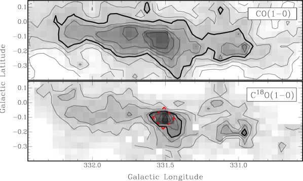
Figure 1.— Maps of velocity integrated emission, in the range -117.7 to -73.2. km s^-1, of the G331.5$-$0.1 GMC. $Top:$ CO$(1\rightarrow$0). Contour levels are drawn from 20% (3$\sigma$) to 90%, in steps of 10%, of the peak intensity (297.6 K km s^-1.). $Bottom:$ C¹⁸O$(1\rightarrow$0). Contour levels are drawn from 20% (4$\sigma$) to 90%, in steps of 10%, of the peak intensity (19.6 K km s^-1). The 50% emission in each map is drawn with a thicker contour. A 7′$\times$7′ red dashed box, oriented in equatorial coordinates, is drawn toward the 70% emission contour in the C¹⁸O$(1\rightarrow$0) map. This area is considered as the central region of this cloud.

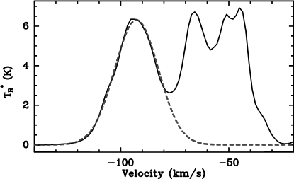
Figure 2.— Average profile of the CO$(1\rightarrow$0) emission over the whole GMC. The dashed line corresponds to the gaussian fit of the spectrum on the velocity range of the G331.5$-$0.1 GMC. The parameters of the gaussian fit are $v_{0}=-92.8\pm 0.006$ km s^-1, $\Delta v=23.8\pm 0.017$ km s^-1 and $T_{peak}=6.31$ K.

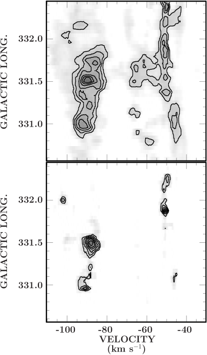
Figure 3.— Position-velocity maps of the CO$(1\rightarrow$0) ($top$) and C¹⁸O$(1\rightarrow$0) emission ($bottom$) integrated between -0.21 and -0.04 in Galactic Latitude. Contour levels are drawn at 40% to 90%, in steps of 10%, of the peak intensity (11.5 K km s^-1 for CO and 0.78 K km s^-1 for C¹⁸O). The C¹⁸O shows a clear component between $l=331.3\arcdeg$ and $l=331.6\arcdeg$ at $\sim-90$ km s^-1.

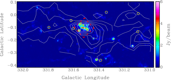
Figure 4.— Map of dust continuum emission at 0.87 mm from ATLASGAL towards the Norma spiral arm tangent region. Overlaid in grey is the contour map of the C¹⁸O$(1\rightarrow$0) emission integrated over the velocity range from -117.7 to -73.2 km s^-1. Contour levels are from 20% to 90%, in intervals of 10%, of the peak intensity 19.6 K km s^-1. The red dashed box, 7′$\times$7′ in size (15$\times$15 pc² at a distance of 7.5 kpc) and oriented in equatorial coordinates, shows the defined central region of the G331.5$-$0.1 GMC. The yellow circles show the position of the RMS sources in this region: G331.0890+00.0163A, G331.0890+00.0163B, G331.0931-00.1303, G331.3865-00.3598, G331.4117+00.0154, G331.4181-00.3546, G331.4904-00.1173, G331.5414-00.0675, G331.5582-00.1206, G331.6035-00.1081, G331.6191-00.0442A, G331.6191-00.0442B, and G331.7953-00.0979.

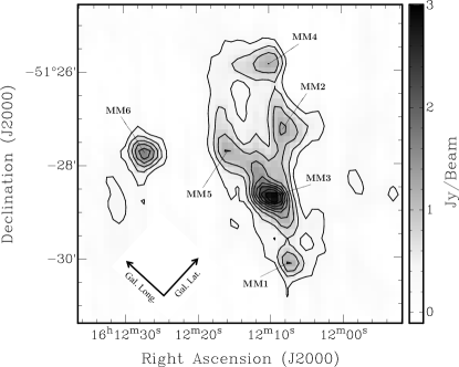
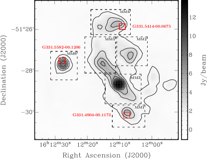
Figure 5.— Maps of the dust continuum emission of the central region of the G331.5$-$0.1 GMC. $Top$: Map of the 1.2 mm emission observed with SIMBA. The angular resolution is 24″. Contour levels are from 10% (3$\sigma$) to 90%, in steps of 10%, of the peak intensity of 2.9 Jy beam^-1. The peak position of millimeter clumps MM1 through MM6, and the Galactic latitude and longitude directions are shown in this map. $Bottom$: Map of the 0.87 mm emission observed with LABOCA. The angular resolution is 18.6″. Contours levels are from 10% (4$\sigma$) to 90%, in steps of 10%, of the peak intensity of 13.8 Jy beam^-1. Dashed boxes in this map show the considered area of each millimeter clump for spectral energy distribution analysis. Red boxes mark the position of RMS sources in the region. The size of these red boxes is 18″$\times$18″ to account for the beam size of the RMS catalog.

Figure 6.— Spectra observed at the peak position of the millimeter clumps MM1 through MM6. The transition is given in the upper right corner. These spectra indicate that the emission arises from two different components: a high velocity component at v=-88.9 km s^-1, and a low velocity component at v=-100.8 km s^-1, indicated with vertical dotted lines. Molecular sources associated with millimeter clumps MM2, MM3, MM4 and MM5 are part of a single structure at high velocity that we defined as the complex of clumps.

Figure 7.— SiO and SO spectra observed toward the peak position of clump MM3, which is associated with the high-velocity molecular outflow G331.512-0.103. Transitions are given in the upper right corner. The vertical dotted line indicates the ambient gas velocity.

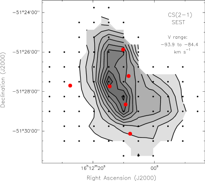
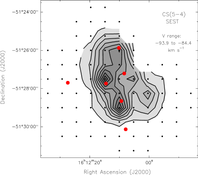
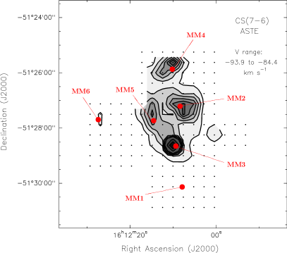
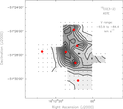
Figure 8.— Contour maps of velocity-integrated emission, in the range from -93.9 to -84.4 km s^-1  from the central region of the G331.5$-$0.1 molecular cloud in four different transitions. For the CS$(7\rightarrow$6) map, the contour levels are drawn at 5%, 10%, 15%, 20%, 25%, 30%, 50% and 70% of the peak flux density 25.6 K km s^-1. For CS$(2\rightarrow$1), CS$(5\rightarrow$4) and ¹³CO$(3\rightarrow$2) maps, the contours are drawn at 10% to 90%, with interval of 10%, of the peak intensity. For CS$(2\rightarrow$1), CS$(5\rightarrow$4) and ¹³CO$(3\rightarrow$2), the peak intensities are 15.3, 5.3 and 161.7 K km s^-1, respectively. The red points show the peak positions of the millimeter clumps MM1 through MM6, as is labeled in the CS$(7\rightarrow$6) contour map. Molecular sources associated with millimeter clumps MM2, MM3, MM4 and MM5 are part of a single structure at high velocity that we defined as the complex of clumps.

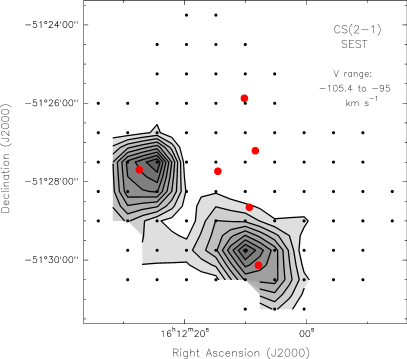
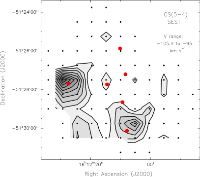
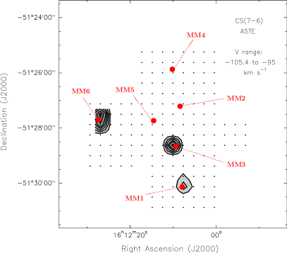
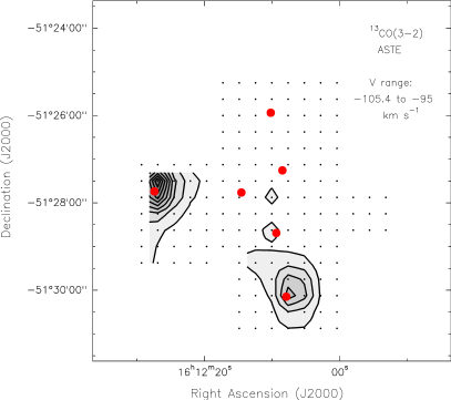
Figure 9.— Contour maps of velocity-integrated emission, in the range between -105.4 and -95 km s^-1, from the central region of the G331.5$-$0.1 molecular cloud in four different transitions. For the CS$(7\rightarrow$6) map, the contour levels are drawn at 10%, 20%, 30%, 40%, 50%, 70% and 90% of the peak flux density 14.0 K km s^-1. For CS$(2\rightarrow$1), CS$(5\rightarrow$4) and ¹³CO$(3\rightarrow$2)maps, the contours are drawn at 10% to 90%, with interval of 10%, of the peak intensity. For CS$(2\rightarrow$1), the peak intensity is 5.2 K km s^-1. For CS$(5\rightarrow$4), the peak intensity is 1.4 K km s^-1. For ¹³CO$(3\rightarrow$2), the peak intensity is 86.7 K km s^-1. The red points show the peak positions of the millimeter clumps MM1 through MM6, as is labeled in the CS$(7\rightarrow$6) contour map. The emission observed in the CS$(7\rightarrow$6) map at $\alpha_{2000}=16^{h}12^{m}10.13^{s}$ and $\delta_{2000}=-51\arcdeg 28\arcmin 37.5\arcsec$ (toward the MM3 point) is related with the emission integration on the blue wing of the G331.512-0.103 outflow.

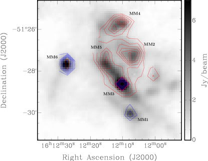
Figure 10.— 0.87 mm greyscale image of the central region of the G331.5$-$0.1 GMC, overlaid with CS velocity integrated contour map. The contour levels are drawn at 5%, 10%, 15%, 20%, 25%, 30%, 50% and 70% of the peak flux density 25.6 K km s^-1. The red contours show the integrated emission in the high velocity component of the spectra, integrated between -93.9 and -84.4 km s^-1. The blue contours show the low velocity component, integrated between -105.4 and -95 km s^-1. Labels MM1 through MM6 show the associated millimeter clump for each CS source. Molecular sources associated with millimeter clumps MM2, MM3, MM4 and MM5 are part of a single structure at high velocity that we defined as the complex of clumps.

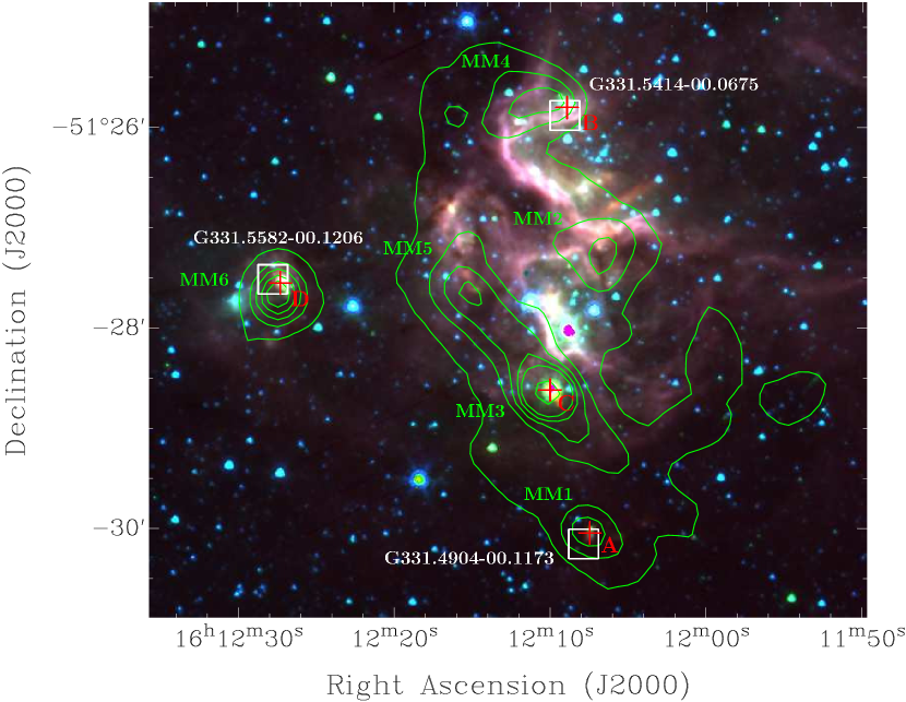
Figure 11.— Contour map of the 0.87 mm continuum emission from the G331.5-0.1 region overlaid on a three color image of the mid infrared emission, made using the IRAC filters 1 (3.6 $\mu$m, blue), 2 (4.5 $\mu$m, green) and 4 (8 $\mu$m, red). Contour levels are drawn at 10%, 20%, 30%, 40%, 50% and 90% of the peak flux density 13.8 Jy beam^-1. Millimeter sources are labeled in the map with MM1, MM2, MM3, MM4, MM5 and MM6. Red crosses mark the positions of the four radio emission components in the central region of the G331.5$-$0.1 GMC (A, B, C and D). Component B and D are associated with methanol and OH masers. Component C is associated only with OH maser emission. White boxes mark the position of the three RMS sources in the region (G331.4904-00.1173, G331.5414-00.0675 and G331.5582-00.1206). The RMS box sizes are 18″ to account for the beam of MSX observation.

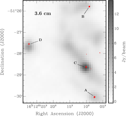
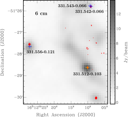
Figure 12.— Contour maps of the radio emission from the G331.5$-$0.1GMC central region at 3.6 cm (top) and 6 cm (bottom), overlaid on 0.87 mm continuum emission. The contours are drawn at 10%, 30%, 60% and 90% of the peak flux. For the 6 cm map, the peak intensity is 153.0 mJy beam^-1, rms noise is 1.04 mJy beam^-1. For the 3.6 cm map, the peak intensity is 159.5 mJy beam^-1, rms noise is 1.09 mJy beam^-1. The blue crosses in the 6 cm map show the position of methanol masers in the central region of the G331.5$-$0.1 GMC. All methanol masers here are associated with OH masers. The yellow cross shows the position of the OH maser, without methanol counterpart, toward the G331.512-0.103 outflow.

Figure 13.— Spectral energy distributions at short frequency for each radio component found in the central region of the G331.5$-$0.1 GMC. For components B and C, the dotted line is a fit of the spectrum using modified blackbody function of the form $B_{\nu}(T_{e})[1-exp(-\tau_{\nu})]$, with $\tau_{\nu}\propto T_{e}^{-1.35}\nu^{-2.1}EM$. The emission measure $EM$ is in units of [pc cm${}^{-6}]$. The $T_{e}$ considered is 10000 K. The spectral index of components B and C are 0.8$\pm$0.2 and 1.2$\pm$0.2, respectively.

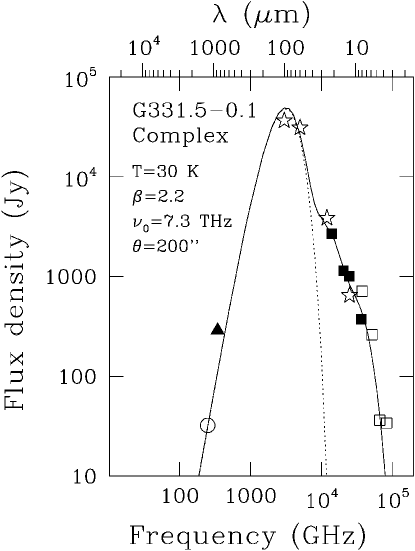
Figure 14.— Spectral energy distribution of the region harboring the G331.5$-$0.1 complex of clumps. From left to right, the circle marks the SIMBA flux, the triangle the LABOCA, the stars mark IRAS fluxes, filled-squares MSX fluxes, and open-squares SPITZER fluxes. The solid curve is a fit to the spectrum using three modified blackbody functions of the form $B_{\nu}(T_{e})[1-exp\left(-(\nu/\nu_{0})^{\beta}\right)]$, with different temperatures (cold, warm and hot components). The fitted parameters of the cold component (represented as the dotted line) are listed.

Figure 15.— Spectral energy distributions of each millimeter clump in the G331.5$-$0.1 central region. The symbols are the same as in Fig. 14. The solid curve is a fit to the spectrum using two modified blackbody functions of the form $B_{\nu}(T_{e})[1-exp\left(-(\nu/\nu_{0})^{\beta}\right)]$, with different temperatures (cold and warm components). In the case of MM1, only on modified black function was considered. The fitted parameters of the cold component (represented as the dotted line) are listed on the upper left.

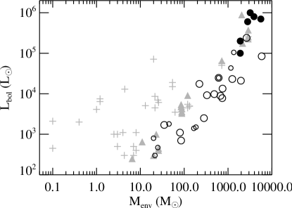
Figure 16.— $L_{bol}-M_{env}$ diagram for the six millimeter clumps (MM1-MM6) in the G331.5$-$0.1 GMC central region (filled black circles), together with sources from Molinari et al. (2008). From Molinari et al. sample, MM sources are represented as open circles (small representing MM-S sources), IR-P sources are shown in grey filled triangles and IR-S are indicated in crosses.

Appendix A Online material

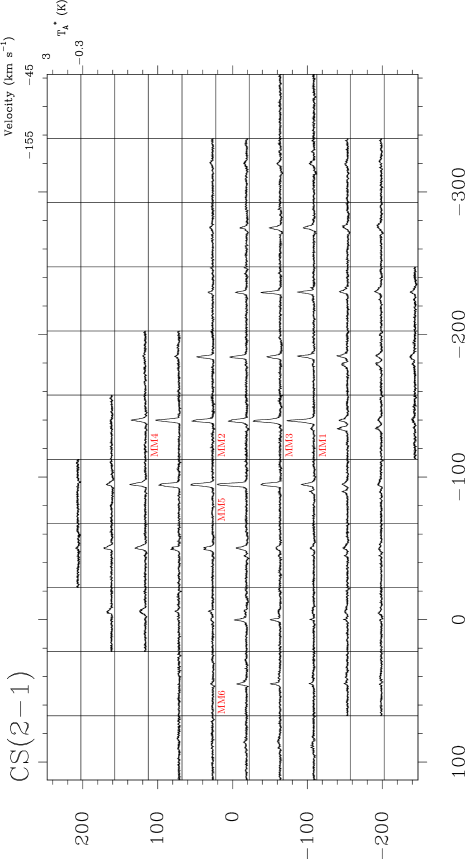
Figure A1.— Observed spectra of the CS$(2\rightarrow$1) line emissions toward the G331.5$-$0.1 GMC central region. The grid spacing is 45″. Offsets are from the reference position at $\alpha_{2000}=16^{h}12^{m}24.5^{s}$ and $\delta_{2000}=-51\arcdeg 27\arcmin 29.98\arcsec$. In each box the velocity scale ranges from -155 to -45 km s^-1. The antenna temperature scale is from -0.3 to 3 K. The labels MM1 to MM6 show the positions in the grid closer to the peak position of the millimeter clumps, defined in section 3.2.1.

Figure A2.— Observed spectra of the CS$(5\rightarrow$4) line emissions toward the G331.5$-$0.1 GMC central region. The grid spacing is 45″. Offsets are from the reference position at $\alpha_{2000}=16^{h}12^{m}24.5^{s}$ and $\delta_{2000}=-51\arcdeg 27\arcmin 29.98\arcsec$. In each box the velocity scale ranges from -155 to -45 km s^-1. The antenna temperature scale is from -0.3 to 1.2 K. The labels MM1 to MM6 show the positions in the grid closer to the peak position of the millimeter clumps, defined in section 3.2.1.

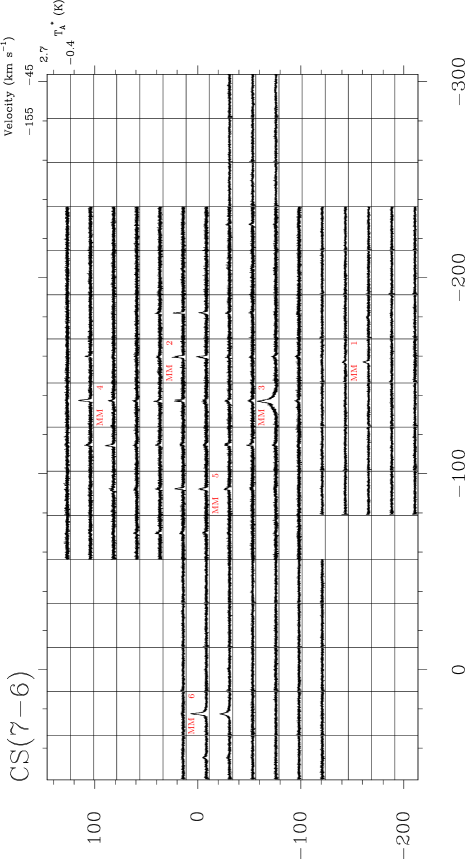
Figure A3.— Observed spectra of the CS$(7\rightarrow$6) line emissions toward the G331.5$-$0.1 central region. The grid spacing is 22.5″. Offsets are from the reference position at $\alpha_{2000}=16^{h}12^{m}24.5^{s}$ and $\delta_{2000}=-51\arcdeg 27\arcmin 29.9\arcsec$. In each box the velocity scale ranges from -155 to -45 km s^-1. The antenna temperature scale is from -0.4 to 2.7 K. The labels MM1 to MM6 show the positions in the grid closer to the peak position of the millimeter clumps, defined in section 3.2.1.

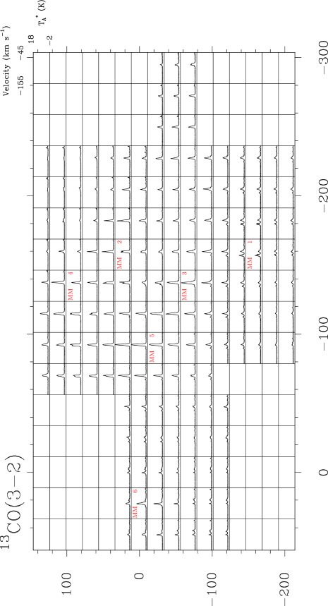
Figure A4.— Observed spectra of the ¹³CO$(3\rightarrow$2) line emissions toward the G331.5$-$0.1 central region. The grid spacing is 22.5″. Offsets are from the reference position at $\alpha_{2000}=16^{h}12^{m}24.5^{s}$ and $\delta_{2000}=-51\arcdeg 27\arcmin 29.9\arcsec$. In each box the velocity scale ranges from -155 to -45 km s^-1. The antenna temperature scale is from -2 to 18 K. The labels MM1 to MM6 show the positions in the grid closer to the peak position of the millimeter clumps, defined in section 3.2.1.

References

- Alvarez et al. (1990) Alvarez, H., May, J., & Bronfman, L. 1990, ApJ, 348, 495
- Bartkiewicz & van Langevelde (2012) Bartkiewicz, A., & van Langevelde, H. J. 2012, IAU Symposium, 287, 117
- Bally et al. (2005) Bally, J., Moeckel, N., & Throop, H. 2005, Chondrites and the Protoplanetary Disk, 341, 81
- Blake et al. (1987) Blake, G. A., Sutton, E. C., Masson, C. R., & Phillips, T. G. 1987, ApJ, 315 621
- Bourke et al. (1997) Bourke, T. L., Garay, G., Lehtinen, K. K., et al. 1997, ApJ, 476, 781
- Bronfman et al. (1985) Bronfman, L., Cohen, R. S., Thaddeus, P., & Alvarez, H. 1985, The Milky Way Galaxy, 106, 331
- Bronfman et al. (1989) Bronfman, L., Alvarez, H., Cohen, R. S., & Thaddeus, P. 1989, ApJS, 71, 481
- Bronfman et al. (1996) Bronfman, L., Nyman, L.-A., & May, J. 1996, A&AS, 115, 81
- Bronfman et al. (2000) Bronfman, L., Casassus, S., May, J., & Nyman, L.-Å. 2000, A&A, 358, 521
- Bronfman et al. (2008) Bronfman, L., Garay, G., Merello, M., et al. 2008, ApJ, 672, 391
- Caswell et al. (1980) Caswell, J. L., Haynes, R. F., & Goss, W. M. 1980, AuJPh, 33, 639
- Caswell & Haynes (1987) Caswell, J. L., & Haynes, R. F. 1987, A&A, 171, 261
- Caswell et al. (1995) Caswell, J. L., Vaile, R. A., Ellingsen, S. P., Whiteoak, J. B., & Norris, R. P. 1995, MNRAS, 272, 96
- Caswell (1997) Caswell, J. L. 1997, MNRAS, 289, 203
- Caswell (1998) Caswell, J. L. 1998, MNRAS, 297, 215
- Caswell (2009) Caswell, J. L. 2009, PASA, 26, 454
- Caswell et al. (2011) Caswell, J. L., Fuller, G. A., Green, J. A., et al. 2011, MNRAS, 417, 1964
- Cesaroni et al. (1991) Cesaroni, R., Walmsley, C. M., Koempe, C., & Churchwell, E. 1991, A&A, 252, 278
- Churchwell et al. (1990) Churchwell, E., Walmsley, C. M., & Cesaroni, R. 1990, A&AS, 83, 119
- Dunham et al. (2011) Dunham, M. K., Rosolowsky, E., Evans, N. J., II, Cyganowski, C., & Urquhart, J. S. 2011, ApJ, 741, 110
- Edgar & Clarke (2004) Edgar, R., & Clarke, C. 2004, MNRAS, 349, 678
- Elia et al. (2010) Elia, D., Schisano, E., Molinari, S., et al. 2010, A&A, 518, L97
- Faúndez et al. (2004) Faúndez, S., Bronfman, L., Garay, G., et al. 2004, A&A, 426, 97
- Fazio et al. (2004) Fazio, G. G., Hora, J. L., Allen, L. E., et al. 2004, ApJS, 154, 10
- Fukui et al. (1991) Fukui, Y., Ogawa, H., Kawabata, K., Mizuno, A., & Sugitani, K. 1991, The Magellanic Clouds, 148, 105
- Fukui & Sakakibara (1992) Fukui, Y., Sakakibara, O. 1992, Mitsubishi Electronic Advance 60, 11
- Furuya (2003) Furuya, R. S. 2003, Galactic Star Formation Across the Stellar Mass Spectrum, 287, 367
- Garay & Lizano (1999) Garay, G., & Lizano, S. 1999, PASP, 111, 1049
- Garay et al. (2002) Garay, G., Brooks, K. J., Mardones, D., Norris, R. P., & Burton, M. G. 2002, ApJ, 579, 678
- Goss et al. (1970) Goss, W. M., Manchester, R. N., & Robinson, B. J. 1970, AuJPh, 23, 559
- Goss et al. (1972) Goss, W. M., Radhakrishnan, V., Brooks, J. W., & Murray, J. D. 1972, ApJS, 24, 123
- Gottlieb et al. (1978) Gottlieb, C. A, Gottlieb,E. W., Litvak, M. M., Ball, J. A., & Penfield, H. 1978, ApJ, 219, 77
- Heiderman et al. (2010) Heiderman, A., Evans, N. J., II, Allen, L. E., Huard, T., & Heyer, M. 2010, ApJ, 723, 1019
- Jones & Dickey (2012) Jones, C., & Dickey, J. M. 2012, ApJ, 753, 62
- Kahn (1974) Kahn, F. D. 1974, A&A, 37, 149
- Kennicutt (1998) Kennicutt, R. C., Jr. 1998, ARA&A, 36, 189
- Kennicutt (2005) Kennicutt, R. C. 2005, Massive Star Birth: A Crossroads of Astrophysics, 227, 3
- Kennicutt & Evans (2012) Kennicutt, R. C., & Evans, N. J. 2012, ARA&A, 50, 531
- Kerr & Knapp (1970) Kerr, F. J., & Knapp, G. R. 1970, AuJPA, 18, 9
- Krumholz & McKee (2008) Krumholz, M. R., & McKee, C. F. 2008, Nature, 451, 1082
- Kuiper et al. (2010) Kuiper, R., Klahr, H., Beuther, H., & Henning, T. 2010, ApJ, 722, 1556
- Lada et al. (2010) Lada, C. J., Lombardi, M., & Alves, J. F. 2010, ApJ, 724, 687
- Larson & Starrfield (1971) Larson, R. B., & Starrfield, S. 1971, A&A, 13, 190
- Linke et al. (1979) Linke,R. A., Frerking, M. A., & Thaddeus, P. 1979, ApJ, 234, L139
- Martin-Pintado et al. (1992) Martin-Pintado, J., Bachiller, R., & Fuente, A. 1992, A&A, 254, 315
- McKee & Ostriker (2007) McKee, C. F., & Ostriker, E. C. 2007, ARA&A, 45, 565
- Menten et al. (1986) Menten, K. M., Walmsley, C. M., Henkel, C., et al. 1986, A&A, 169, 271
- Miettinen et al. (2006) Miettinen, O., Harju, J., Haikala, L. K., & Pomrén, C. 2006, A&A, 460, 721
- Mill et al. (1994) Mill, J. D., O’Neil, R. R., Price, S., et al. 1994, JSpRo, 31, 900
- Molinari et al. (2008) Molinari, S., Pezzuto, S., Cesaroni, R., et al. 2008, A&A, 481, 345
- Myers (1995) Myers, P. C. 1995, Molecular Clouds and Star Formation, 47
- Neugebauer et al. (1984) Neugebauer, G., Habing, H. J., van Duinen, R., et al. 1984, ApJ, 278, L1
- Ogawa et al. (1990) Ogawa, H., Mizuno, A., Ishikawa, H., Fukui, Y., & Hoko, H. 1990, IJIMW, 11, 717
- Ossenkopf & Henning (1994) Ossenkopf, V., & Henning, T. 1994, A&A, 291, 943
- Panagia (1973) Panagia, N. 1973, AJ, 78, 929
- Pestalozzi et al. (2005) Pestalozzi, M. R., Minier, V., & Booth, R. S. 2005, A&A, 432, 737
- Plambeck et al. (1982) Plambeck, R. L., Wright, M. C. H., Welch, W. J., et al. 1982, ApJ, 259, 617
- Plume et al. (1992) Plume, R., Jaffe, D. T., & Evans, N. J., II. 1992, ApJS, 78, 505
- Reynolds (1986) Reynolds, S. P. 1986, ApJ, 304, 713
- Rydbeck et al. (1980) Rydbeck, O. E. H., Hjalmarson, A., Rydbeck, G., et al. 1980, ApJ, 235, L171
- Sault et al. (1995) Sault, R. J., Teuben, P. J., & Wright, M. C. H. 1995, Astronomical Data Analysis Software and Systems IV, 77, 433
- Schilke et al. (1997) Schilke, P., Walmsley, C. M., Pineau des Forets, G., & Flower, D. R. 1997, A&A, 321, 293
- Schuller et al. (2009) Schuller, F., Menten, K. M., Contreras, Y., et al. 2009, A&A, 504, 415
- Shaver & Goss (1970) Shaver, P. A., & Goss, W. M. 1970, AuJPA, 14, 133
- Shirley et al. (2003) Shirley, Y. L., Evans, N. J., II, Young, K. E., Knez, C., & Jaffe, D. T. 2003, ApJS, 149, 375
- Swade (1989) Swade, D. A. 1989, ApJ, 345, 828
- Szymczak et al. (2002) Szymczak, M., Kus, A. J., Hrynek, G., Kěpa, A., & Pazderski, E. 2002, A&A, 392, 277
- Urquhart et al. (2008) Urquhart, J. S., Hoare, M. G., Lumsden, S. L., Oudmaijer, R. D., & Moore, T. J. T. 2008, Massive Star Formation: Observations Confront Theory, 387, 381
- Welch et al. (1981) Welch, W. J., Wright, M. C. H., Plambeck, R. L., Bieging, J. H., & Baud, B. 1981, ApJ, 245, L87
- Williams et al. (2000) Williams, J. P., Blitz, L., & McKee, C. F. 2000, Protostars and Planets IV, 97
- Wilson & Rood (1994) Wilson, T. L., & Rood, R. 1994, ARA&A, 32, 191
- Wilson et al. (2009) Wilson, T. L., Rohlfs, K., Hüttemeister, S. 2009, Tools of Radio Astronomy, by Thomas L. Wilson; Kristen Rohlfs and Susanne Hüttemeister. ISBN 978-3-540-85121-9. Published by Springer-Verlag, Berlin, Germany, 2009.,
- Wolfire & Cassinelli (1987) Wolfire, M. G., & Cassinelli, J. P. 1987, ApJ, 319, 850
- Yorke & Kruegel (1977) Yorke, H. W., & Kruegel, E. 1977, A&A, 54, 183
- Zinnecker & Yorke (2007) Zinnecker, H., & Yorke, H. W. 2007, ARA&A, 45, 481