A panchromatic view of the restless SN 2009ip reveals the explosive ejection of a massive star envelope

Abstract

The 2012 explosion of SN 2009ip raises questions about our understanding of the late stages of massive star evolution. Here we present a comprehensive study of SN 2009ip during its remarkable re-brightening(s). High-cadence photometric and spectroscopic observations from the GeV to the radio band obtained from a variety of ground-based and space facilities (including the VLA, Swift, Fermi, HST and XMM) constrain SN 2009ip to be a low energy ($E\sim 10^{50}$ erg for an ejecta mass $\sim 0.5\,\rm{M_{\sun}}$) and likely asymmetric explosion in a complex medium shaped by multiple eruptions of the restless progenitor star. Most of the energy is radiated as a result of the shock breaking out through a dense shell of material located at $\sim 5\times 10^{14}\,\rm{cm}$ with $M\sim 0.1\,\rm{M_{\sun}}$, ejected by the precursor outburst $\sim 40$ days before the major explosion. We interpret the NIR excess of emission as signature of dust vaporization of material located further out ($R>4\times 10^{15}\,\rm{cm}$), the origin of which has to be connected with documented mass loss episodes in the previous years. Our modeling predicts bright neutrino emission associated with the shock break-out if the cosmic ray energy is comparable to the radiated energy. We connect this phenomenology with the explosive ejection of the outer layers of the massive progenitor star, that later interacted with material deposited in the surroundings by previous eruptions. Future observations will reveal if the luminous blue variable (LBV) progenitor star survived. Irrespective of whether the explosion was terminal, SN 2009ip brought to light the existence of new channels for sustained episodic mass-loss, the physical origin of which has yet to be identified.

1. Introduction

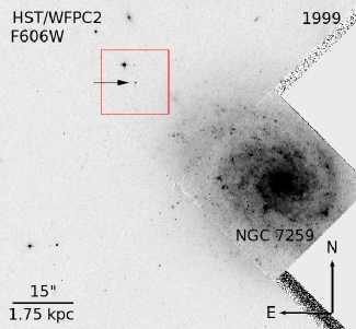
Figure 1.— Hubble Space Telescope (HST) pre-explosion image acquired in 1999 (Program 6359; PI: Stiavelli). The location of the progenitor of SN 2009ip is marked by an arrow. SN 2009ip exploded in the outskirts of its host galaxy NGC 7259 at an angular distance of $\sim 43.4^{\prime\prime}$ from the host center, corresponding to $\sim 5\,\rm{kpc}$.

Standard stellar evolutionary models predict massive stars with $M\gtrsim 40\,\rm{M_{\odot}}$ to spend half a Myr in the Wolf-Rayet (WR) phase before exploding as supernovae (SNe, e.g. Georgy et al. 2012 and references therein). As a result, massive stars are not expected to be H rich at the time of explosion. Yet, recent observations have questioned this picture, revealing the limitations of our current understanding of the last stages of massive star evolution and in particular the uncertainties in the commonly assumed mass loss prescriptions (e.g. Smith & Owocki 2006). Here, we present observations from an extensive, broad-band monitoring campaign of SN 2009ip (Fig. 1) during its double explosion in 2012 that revealed extreme mass-loss properties, raising questions about our understanding of the late stages of massive star evolution.

An increasingly complex picture is emerging connecting SN progenitor stars with explosion properties. The most direct link arguably comes from the detection of progenitor stars in pre-explosion images. These efforts have been successful connecting Type IIP SNe with the death of red supergiants ($M\sim 8-15\,\rm{M_{\sun}}$, Smartt 2009). However, massive progenitor stars have proven to be more elusive (e.g. Kochanek et al. 2008): SN 2005gl constitutes the first direct evidence for a massive ($M>50\,M_{\sun}$) and H rich star to explode as a core-collapse SN, contrary to theoretical expectations (Gal-Yam et al. 2007; Gal-Yam et al. 2009).

SN 2005gl belongs to the class of Type IIn SNe (Schlegel 1990). Their spectra show evidence for strong interaction between the explosion ejecta and a dense circumstellar medium (CSM) previously enriched by mass loss from the progenitor star. In order for the SN to appear as a Type IIn explosion, the mass loss and the core collapse have to be timed, with mass loss occurring in the decades to years before the collapse. This timing requirement constitutes a further challenge to current evolutionary models and emphasizes the importance of the progenitor mass loss in the years before the explosion in determining its observable properties.

Mass loss in massive stars can either occur through steady winds (on a typical time scale of $10^{3}$ yr) or episodic outbursts lasting months to years, reminiscent of Luminous Blue Variable (LBV) eruptions (see Humphreys & Davidson 1994 for a review). SN 2005gl, with its LBV-like progenitor, established the first direct observational connection between SNe IIn and LBVs. On the other hand, there are controversial objects like SN 1961V, highlighting the present difficulty in distinguishing between a giant LBV eruption and a genuine core-collapse explosion even 50 years after the event (Van Dyk & Matheson 2012, Kochanek et al. 2011 and references therein). The dividing line between SNe and impostors can be ambiguous.

Here we report on our extensive multi-wavelength campaign to monitor the evolution of SN 2009ip, which offers an unparalleled opportunity to study the effects and causes of significant mass loss in massive stars in real time. Discovered in 2009 (Maza et al., 2009) in NGC 7259 (spiral galaxy with brightness $M_{\rm{B}}\sim-18$ mag, Lauberts & Valentijn 1989), it was first mistaken as a faint SN candidate (hence the name SN 2009ip). Later observations (Miller et al. 2009; Li et al. 2009; Berger et al. 2009) showed the behavior of SN 2009ip to be consistent instead with that of LBVs. Pre-explosion Hubble Space Telescope (HST) images constrain the progenitor to be a massive star with $M\gtrsim 60\,\rm{M_{\odot}}$ (Smith et al. 2010b, Foley et al. 2011), consistent with an LBV nature. The studies by Smith et al. (2010b) and Foley et al. (2011) showed that SN 2009ip underwent multiple explosions in rapid succession in 2009. Indeed, a number of LBV-like eruptions were also observed in 2010 and 2011: a detailed summary can be found in Levesque et al. (2012) and a historic light-curve is presented by Pastorello et al. (2012). Among the most important findings is the presence of blue-shifted absorption lines corresponding to ejecta traveling at a velocity of $2000-7000\,\rm{km\,s^{-1}}$ during the 2009 outbursts (Smith et al. 2010b, Foley et al. 2011), extending to $v\sim 13000\,\rm{km\,s^{-1}}$ in Semptember 2011 (Pastorello et al., 2012). Velocities this large have never been associated with LBV outbursts to date.

SN 2009ip re-brightened again on 2012 July 24 (Drake et al. 2012), only to dim considerably $\sim 40$ days afterwards (hereafter referred to as the 2012a outburst). The appearance of high-velocity spectral features was first noted by Smith & Mauerhan (2012) on 2012 September 22. This was shortly followed by the major 2012 re-brightening on September 23 (2012b explosion hereafter, Brimacombe 2012, Margutti et al. 2012). SN 2009ip reached $M_{\rm{V}}<-18\,\rm{mag}$ at this time, consequently questioning the actual survival of the progenitor star: SN or impostor? (Pastorello et al. 2012; Prieto et al. 2013; Mauerhan et al. 2013; Fraser et al. 2013; Soker & Kashi 2013).

Here we present a comprehensive study of SN 2009ip during its remarkable evolution in 2012. Using observations spanning more than 15 decades in wavelength, from the GeV to the radio band, we constrain the properties of the explosion and its complex environment, identify characteristic time scales that regulate the mass loss history of the progenitor star, and study the process of dust vaporization in the progenitor surroundings. We further predict the neutrino emission associated with this transient.

This paper is organized as follows. In Section 2-6 we describe our follow up campaign and derive the observables that can be directly constrained by our data. In Section 7 we present the properties of the explosion and environment that can be inferred from the data under reasonable assumptions. In Section 8 we address the major questions raised by this explosion and speculate about answers. Conclusions are drawn in Section 9.

Uncertainties are $1\sigma$ unless stated otherwise. Following Foley et al. (2011) we adopt a distance modulus of $\mu=32.05\,\rm{mag}$ corresponding to a distance $d_{\rm{L}}=24$ Mpc and a Milky Way extinction $E(B-V)=0.019$ mag (Schlegel et al., 1998) with no additional host galaxy or circumstellar extinction. From VLT-Xshooter high-resolution spectroscopy our best estimate for the redshift of the explosion is $z=0.005720$, which we adopt through out the paper. We use $U$, $B$ and $V$ for the Johnson filters. u, b and v refer to Swift-UVOT filters. Standard cosmological quantities have been adopted: $H_{0}=71\,\rm{km\,s^{-1}\,Mpc^{-1}}$, $\Omega_{\Lambda}=0.73$, $\Omega_{\rm{M}}=0.27$. All dates are in UT and are reported with respect to MJD 56203 (2012 October 3) which corresponds to the UV peak ($t_{\rm{pk}}$).

2. Observations and data analysis

Our campaign includes data from the radio band to the GeV range. We first describe the data acquisition and reduction in the UV, optical and NIR bands (which are dominated by thermal emission processes) and then describe the radio, X-ray and GeV observations, which sample the portion of the spectrum where non-thermal processes are likely to dominate.

2.1. UV photometry

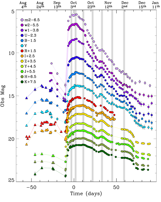
Figure 2.— Photometric evolution of SN 2009ip in the UV, optical and NIR (filled circles). We add NIR observations of the 2012a outburst published by Pastorello et al. (2012) for $t<-10\,\rm{days}$ (triangles) together with R and I-band photometry from Prieto et al. (2013) obtained during the rise-time (triangles). The shaded gray vertical bands mark the time of observed bumps in the light-curve. Our late time UVOT photometry from April 2013 is not shown here.

We initiated our Swift-UVOT (Roming et al., 2005) photometric campaign on 2009 September 10 and followed the evolution of SN 2009ip in the 6 UVOT filters up until April 2013. Swift-UVOT observations span the wavelength range $\lambda_{c}=1928$ Å  (w2 filter) - $\lambda_{c}=5468$ Å  (v filter, central wavelength listed, see Poole et al. 2008 for details). Data have been analyzed following the prescriptions by Brown et al. (2009). We used different apertures during the fading of the 2012a outburst to maximize the signal-to-noise ratio and limit the contamination by a nearby star. For the 2012a event we used a $3^{\prime\prime}$ aperture for the b and v filters; $4^{\prime\prime}$ for the u filter and $5^{\prime\prime}$ for the UV filters. We correct for PSF losses following standard prescriptions. At peak SN 2009ip reaches u$\sim 12.5$ mag potentially at risk for major coincidence losses. For this reason we requested a smaller readout region around maximum light. Our final photometry is reported in Table 5 and shown in Fig. 2. The photometry is based on the UVOT photometric system (Poole et al. 2008) and the revised zero-points of Breeveld et al. (2011).

2.2. UV spectroscopy: Swift-UVOT and HST

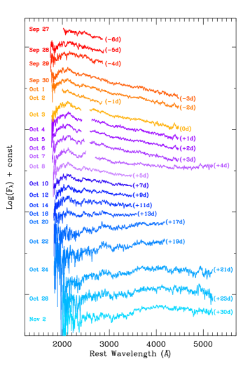
Figure 3.— Sequence of Swift-UVOT spectra of SN 2009ip covering the rise time (red to orange), peak time (shades of purple) and decay time (shades of blue) of the 2012b explosion.

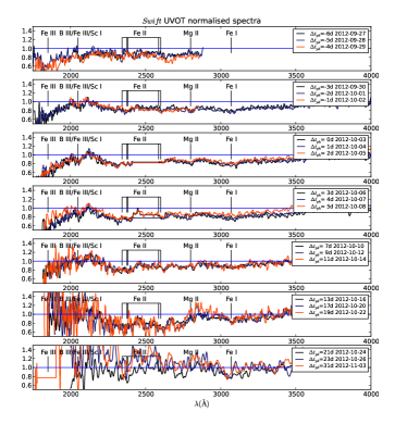
Figure 4.— UV portion of the Swift-UVOT spectra re-normalized using the black-body fits of Sect. 3, with identifications. As time proceeds Fe III absorption features become weaker while Fe II develops stronger absorption features, consistent with the progressive decrease of the black-body temperature with time (Fig. 11).

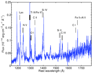
Figure 5.— Upper panel: HST-STIS spectrum obtained on 2012 October 29 ($t_{\rm{pk}}+26$ days). The C III] and Si III] identifications are in a noisy part of the spectrum and are therefore uncertain. Lower panel: HST-COS spectrum obtained on 2012 November 6 ($t_{\rm{pk}}+34$ days).

Motivated by the bright UV emission and very blue colors of SN 2009ip we initiated extensive UV spectral monitoring on 2012 September 27, $\sim 6$ days before maximum UV light (2012b explosion). Our campaign includes a total of 22 UVOT UV-grism low-resolution spectra and two epochs of Hubble Space Telescope (HST) observations (PI R. Kirshner), covering the period $-6\,\rm{days}<t-t_{\rm{pk}}<+34\,\rm{days}$.

Starting on 2012 September 27 ($t_{\rm{pk}}-6$ days), a series of spectra were taken with the Swift UVOT UV grism, with a cadence of one to two days, until 2012 October 28 ($t_{\rm{pk}}+25$ days), with a final long observation on 2012 November 2 ($t_{\rm{pk}}+30$ days).

Details are given in Table 2. Over the course of the month the available roll angles changed. The roll angle controls the position of the grism spectrum relative to the strong zeroth orders from background stars in the grism image. The best roll angle had the spectrum lying close to the first order of some other sources, while some zeroth orders contaminated part of the spectrum in some observations. Finally, the second order overlap limits the usefulness of the red part of the UV grism spectrum. To obtain the best possible uncontaminated spectra range, the spectra were observed at a position on the detector where the second order lies next to the first order, increasing the good, uncontaminated part of the first order from about 1900 Å  to 4500 Å.

The spectra were extracted from the image using the UVOTPY package. The wavelength anchor and flux calibration were the recent updates valid for locations other than the default position in the center (Kuin et al. in prep., details can be found on-line). The spectra were extracted for a slit with the default 2.5$\,\sigma$ aperture and a 1$\,\sigma$ aperture. An aperture correction was made to the 1$\,\sigma$ aperture spectra which were used. The 1$\,\sigma$ aperture does not suffer as much from contamination as the larger aperture. Contamination from other sources and orders is readily seen when comparing the extractions of the two apertures. The wavelength accuracy is 20 Å  (1$\,\sigma$), the flux accuracy (systematic) is within 10%, while the resolution is $R\sim 75-110$ depending on the wavelength range. The error in the flux was computed from the Poisson noise in the data, as well as from the consistency of between the spectra extracted from the images on one day. The sequence of Swift-UVOT spectra is shown in Fig. 3. Figure 4 shows the UV portion of the spectra, re-normalized using the black-body fits derived in Sec. 3.

Starting from November 2012 SN 2009ip is too faint for Swift-UVOT spectroscopic observations. We continued our UV spectroscopic campaign with HST (Fig. 5). Observations with the Space Telescope Imaging Spectrograph (STIS) were taken on 2012 October 29 ($t_{\rm{pk}}+26$ days) using aperture 52x0.2E1 with gratings G230LB, G430L and G750L with exposures times of 1200 s, 400 s and 100 s, respectively. The STIS 2-D images were cleaned of cosmic rays and dead pixel signatures before extraction. The extracted spectra were then matched in flux to the STSDAS/STIS pipeline 1-D data product. The spectrum is shown in Fig. 5. Further HST-COS data were acquired on 2012 November 6 ($t_{\rm{pk}}+34$ days, Fig. 5, lower panel). Observations with the Cosmic Origin Spectrograph (COS) were acquired using MIRROR A + bright object aperture for 250 s. The COS data were then reprocessed with the COS calibration pipeline, CALCOS v2.13.6, and combined with the custom IDL co-addition procedure described by Danforth et al. (2010) and Shull et al. (2010). The co-addition routine interpolates all detector segments and grating settings onto a common wavelength grid, and makes a correction for the detector quantum efficiency enhancement grid. No correction for the detector hex pattern is performed. Data were obtained in four central wavelength settings in each far-UV grating mode (1291, 1300, 1309, and 1318 with G130M and 1577, 1589, 1600, and 1611 with G160M) at the default focal-plane split position. The total exposure time for the far-UV observation was 3100 s and 3700 s for near-UV.

2.3. Optical photometry

Observations in the v, b and u filters were obtained with Swift-UVOT and reduced as explained in Sec. 2.1. The results from our observations are listed in Table 5. In Fig. 2 we apply a dynamical color term correction to the UVOT v, b and u filters to plot the equivalent Johnson magnitudes as obtained following the prescriptions by Poole et al. (2008). This is a minor correction to the measured magnitudes and it is not responsible for the observed light-curve bumps.

We complement our data set with R and I band photometry obtained with the UIS Barber Observatory 20-inch telescope (Pleasant Plains, IL), a 0.40 m f/6.8 refracting telescope operated by Josch Hambasch at the Remote Observatory Atacama Desert, a Celestron C9.25 operated by TG Tan (Perth, Australia), and a C11 Schmidt-Cassegrain telescope operated by Ivan Curtis (Adelaide, Australia). Exposure times ranged from 120 s to 600 s. Images were reduced following standard procedure. Each individual image in the series was measured and then averaged together over the course of the night. The brightness was measured using circular apertures adjusted for seeing conditions and sky background from an annulus set around each aperture. Twenty comparison stars within 10^′ of the target were selected from the AAVSO Photometric All-Sky Survey. Statistical errors in the photometry for individual images were typically 0.05 magnitudes or less. Photometry taken by different telescopes on the same night are comparable within the errors. Finally, the photometry was corrected to the photometric system of Pastorello et al. (2012) using the corrections of dR = +0.046 and dI = +0.023 (Pastorello, personal communication). R and I band photometry is reported in Table 6.

A single, late-time ($t_{\rm{pk}}+190$ days) V-band observation was obtained with the Inamori-Magellan Areal Camera and Spectrograph (IMACS, Dressler et al. 2006) mounted on the Magellan/Baade $6.5$-m telescope on 2013 Apr 11.40. Using standard tasks in IRAF to perform aperture photometry and calibrating to a standard star field at similar airmass, we measure $V=19.65\pm 0.02$ mag (exposure time of 90 s).

2.4. Optical spectroscopy

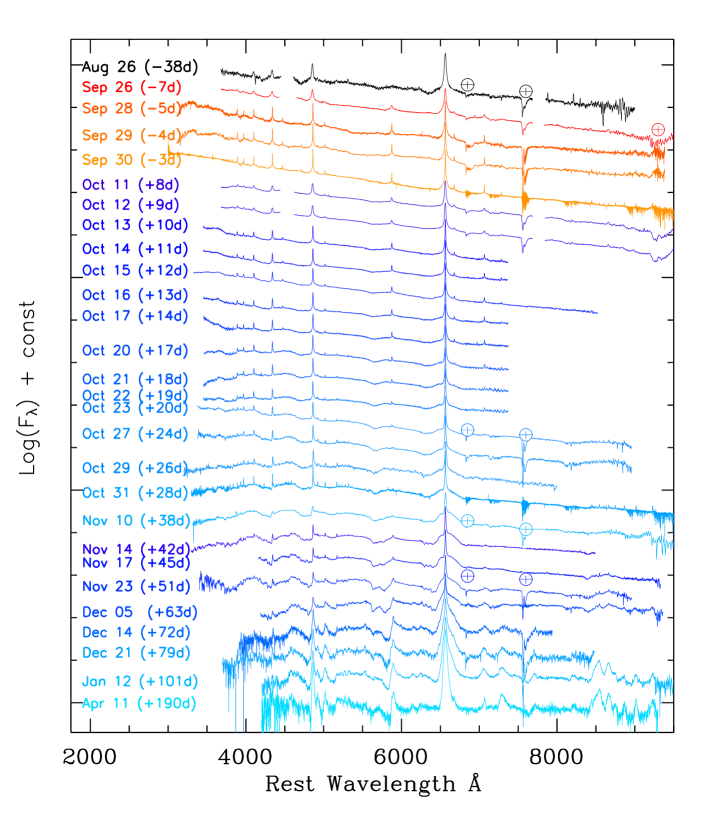
Figure 6.— Optical spectra of SN 2009ip. Shades of red (blue) are used for spectra obtained during the rise time (decay time) of the 2012b explosion. Black is used for the 2012a outburst.

We obtained 28 epochs of optical spectroscopy of SN 2009ip covering the time period 2012 August 26 to 2013 April 11 using a number of facilities (see Table 3).

SN 2009ip was observed with the MagE (Magellan Echellette) Spectrograph mounted on the 6.5-m Magellan/Clay Telescope at Las Campanas Observatory. Data reduction was performed using a combination of Jack Baldwin’s mtools package and IRAF echelle tasks, as described in Massey et al. (2012). Optical spectra were obtained at the F.  L.  Whipple Observatory (FLWO) 1.5-m Tillinghast telescope on several epochs using the FAST spectrograph (Fabricant et al., 1998). Data were reduced using a combination of standard IRAF and custom IDL procedures (Matheson et al., 2005). Low and medium resolution spectroscopy was obtained with the Robert Stobie Spectrograph mounted on the Southern African Large Telescope (SALT/RSS) at the South African Astronomical Observatory (SAAO) in Sutherland, South Africa. Additional spectroscopy was acquired with the Goodman High Throughput Spectrograph (GHTS) on the SOAR telescope. We also used IMACS mounted on the Magellan telescope and the Low Dispersion Survey Spectrograph 3 (LDSS3) on the Clay telescope (Magellan II). The Multiple Mirror Telescope (MMT) equipped with the “Blue Channel” spectrograph (Schmidt et al., 1989) was used to monitor the spectral evolution of SN 2009ip over several epochs. Further optical spectroscopy was obtained with the R-C CCD Spectrograph (RCSpec) mounted on the Mayall 4.0 m telescope, a Kitt Peak National Observatory (KPNO) facility. Spectra were extracted and calibrated following standard procedures using IRAF routines.

We used the X-shooter echelle spectrograph (D’Odorico et al., 2006) mounted at the Cassegrain focus of the Kueyen unit of the Very Large Telescope (VLT) at the European Southern Observatory (ESO) on Cerro Paranal (Chile) to obtain broad band, high-resolution spectroscopy of SN 2009ip on 2012 September 30 ($t_{\rm{pk}}-3$ days) and October 31 ($t_{\rm{pk}}+28$ days). The spectra were simultaneously observed in three different arms, covering the entire wavelength range 3000–25000 Å: ultra-violet and blue (UVB), visual (VIS) and near-infrared (NIR) wavebands. The main dispersion was achieved through a 180 grooves/mm echelle grating blazed at 41.77^∘ (UVB), 99 grooves/mm echelle grating blazed at 41.77^∘ (VIS) and 55 grooves/mm echelle grating blazed at 47.07^∘ (NIR). Observations were performed at parallactic angle under the following conditions: clear sky, the average seeing was $\sim$ 0.7^′′ and $\sim$ 1.0^′′ and the airmass range was $\sim$ 1.1–1.23. We used the X-shooter pipeline (Modigliani et al., 2010) in physical mode to reduce both SN 2009ip and the standard star spectra to two-dimensional bias-subtracted, flat-field corrected, order rectified and wavelength calibrated spectra in counts. To obtain 1-D spectra the 2-D spectra from the pipeline were optimally extracted (see Horne, 1986) using a custom IDL program. Furthermore, the spectra were slit-loss corrected, flux calibrated and corrected for heliocentric velocities using a custom IDL program. The spectra were not (carefully) telluric corrected. The sequence of optical spectra is shown in Fig. 6.

2.5. NIR photometry

We obtained ZYJHK data using the Wide-field Infrared Camera (WFCAM) on the United Kingdom Infrared Telescope (UKIRT). The observation started on 2012 September 23 ($t_{\rm{pk}}-10$ days), and continued on a nearly daily basis until 2012 December 31($t_{\rm{pk}}+89$ days) when SN 2009ip settled behind the Sun. The data reduction was done through an automatic pipeline of the Cambridge Astronomy Survey Unit. The flux of the object was measured with AUTO-MAG of SExtractor (Bertin & Arnouts, 1996), where the photometric calibration was done using 2MASS stars within a radius of 8 arcmin from SN 2009ip. The 2MASS magnitudes of the stars were converted to the UKIRT system following Hodgkin et al. (2009) and the stars with the magnitude errors smaller than 0.10 mag were used for the photometry calibration, which yields typically 20-30 stars. A more detailed description of the NIR photometry can be found in Im et al. (in preparation).

Additional NIR photometry was obtained with PAIRITEL, the f/13.5 1.3-meter Peters Automated Infrared Imaging TELescope at the Fred Lawrence Whipple Observatory (FLWO) on Mount Hopkins, Arizona (Bloom et al., 2006). PAIRITEL data were processed with a single mosaicking pipeline that co-adds and registers PAIRITEL raw images into mosaics (see Wood-Vasey et al. 2008; Friedman 2012).Aperture photometry with a $3^{\prime\prime}$ aperture was performed at the SN position in the mosaicked images using the IDL routine aper.pro. No aperture corrections or host galaxy subtraction were performed. Figure 2 presents the complete SN 2009ip NIR data set. The PAIRITEL photometry can be found in Table 7. A table will the UKIRT photometry will be published in Im et al. (in preparation).

2.6. NIR spectroscopy

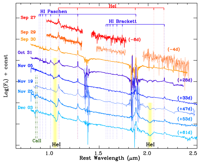
Figure 7.— NIR spectral sequence with line identifications overlaid. The high-resolution spectrum obtained on 2012 November 19 has been smoothed here for display purposes. Shades of red (blue) have been used for spectra obtained during the rise (decay) time. A portion of the VLT/X-shooter spectra is also shown here.

In addition to the X-shooter spectra, early time, low-dispersion ($R\approx 700$) NIR spectra covering 0.9 to 2.4 $\mu\rm{m}$ were obtained with the 2.4m Hiltner telescope at MDM Observatory on 2012 September 27 ($t_{\rm{pk}}-6$ days) and September 29 ($t_{\rm{pk}}-4$ days). The data were collected using TIFKAM, a high-throughput infrared imager and spectrograph with a $1024\times 1024$ Rockwell HgCdTe (HAWAII-1R) detector. The target was dithered along the $0.6^{\prime\prime}$ slit in a ABBA pattern to minimize the effect of detector defects and provide first-order background subtractions. Data reduction followed standard procedures using the IRAF software. Wavelength calibration of the spectra was achieved by observing argon lamps at each position. The spectra were corrected for telluric absorption by observing A0V stars at similar airmasses, and stellar features were removed from the spectra by dividing by an atmospheric model of Vega (Kurucz, 1993).

Additional NIR low-resolution spectroscopy of SN 2009ip was obtained with the Folded-Port Infrared Echellette (FIRE) spectrograph (Simcoe et al., 2013) on the 6.5-m Magellan Baade Telescope, with simultaneous coverage from 0.82 to 2.51 $\mu m$. Spectra were acquired on 2012 November 5, 25 and December 3. The object was nodded along the slit using the ABBA pattern. The slit width was $0.6\arcsec$, yielding $R\approx 500$ in the J band. Data were reduced following the standard procedures described in Vacca et al. (2003), Foley et al. (2012) and Hsiao et al. (2013). An A0V star was observed for telluric corrections. The resulting telluric correction spectrum was also used for the absolute flux calibration.

Moderate-resolution ($R\sim 6000$) NIR spectroscopy was obtained on 2012 November 19 with FIRE. SN 2009ip was observed in high-resolution echellette mode with the $0.6\arcsec$ slit. Eight frames were taken on source with 150 s exposures using ABBA nodding. Data were reduced using a custom-developed IDL pipeline (FIREHOSE), evolved from the MASE suite used for optical echelle reduction (Bochanski et al., 2009). Standard procedures were followed to apply telluric corrections and relative flux calibrations as described above. Finally, the corrected echelle orders were combined into single 1D spectrum for analysis. The complete sequence of NIR spectra is shown in Fig. 7. The observing log can be found in Table 4.

2.7. Millimeter and Radio Observations: CARMA and EVLA

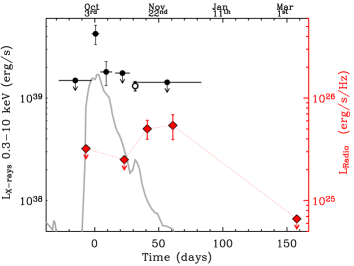
Figure 8.— X-ray (Swift-XRT and XMM-Newton, filled and open circle, respectively) and 9 GHz radio light-curve (red squares, VLA) of SN 2009ip. X-rays are detected when the bolometric luminosity reaches its peak. Radio emission is detected at much later times. A re-scaled version of the bolometric light-curve is also shown for comparison. This plot does not include the late time X-ray limit obtained on 2013 April 4.5 ($t_{\rm{pk}}+183$ days).

Table 1Radio and millimeter observations of SN 2009ip

Date		$F_{\nu}$	$\nu$	Instrument
(UT start time)		($\mu$Jy)	(GHz)
2012 Sep	26.096	$<115.2$	21.25	VLA
2012 Sep	26.096	$<46.5$	8.85	VLA
2012 Sep	26.63	$<66$	18	ATCA
2012 Sep	27.170	$<1000$	84.5	CARMA
2012 Oct	16.049	$<70.5$	21.25	VLA
2012 Oct	17.109	$<104.1$	21.25	VLA
2012 Oct	17.120	$<1500$	84.5	CARMA
2012 Oct	26.036	$<36.3$	8.85	VLA
2012 Nov	6.078	$<59.1$	21.25	VLA
2012 Nov	12.966	$72.6\pm 15.2$	8.85	VLA
2012 Dec	1.987	$<70.5$	21.25	VLA
2012 Dec	2.932	$78.3\pm 21.4$	8.99	VLA
2013 Mar	9.708	$<9.6$	9.00	VLA

Note. — Errors are $1\sigma$ and upper limits are $3\sigma$.

We obtained two sets of millimeter observations at mean frequency of $\sim$84.5 GHz ($\sim$7.5 GHz bandwidth) with the Combined Array for Research in Millimeter Astronomy (CARMA; Bock et al. 2006) around maximum light, beginning 2012 September 27.17 ($t_{\rm{pk}}-6$ days) and 2012 October 17.12 ($t_{\rm{pk}}+14$ days). We utilized 2158-150 and 2258-279 for gain calibration, 2232+117 for bandpass calibration, and Neptune for flux calibration. In $\sim$160 and $\sim$120 min integration time at the position of SN 2009ip, we obtain 3-$\sigma$ upper limits on the flux density of 1.5 and 1.0 mJy, respectively. The overall flux uncertainty with CARMA is $\sim$20%.

We observed the position of SN 2009ip with the Karl G. Jansky Very Large Array (VLA; Perley et al. 2011) on multiple epochs beginning 2012 September 26.10 ($t_{\rm{pk}}-7$ days), with the last epoch beginning 2012 Dec 2.93 ($t_{\rm{pk}}+61$ days). These observations were carried out at 21.25 GHz and 8.85 GHz with 2 GHz bandwidth in the VLA’s most extended configuration (A; maximum baseline length $\sim$36.4 km) except for the first observations, which were obtained in the BnA configuration. In most epochs our observations of flux calibrator, 3C48, were too contaminated with Radio Frequency Interference (RFI). Therefore, upon determining the flux of our gain calibrator J2213-2529 from the best observations of 3C48, we set the flux density of J2213-2529 in every epoch to be 0.65 and 0.63 Jy, for 21.25 and 8.9 GHz, respectively. We note that this assumption might lead to slightly larger absolute flux uncertainties than usual ($\sim$15-20%). In addition, the source-phase calibrator cycle time ($\sim$6 min) was a bit longer than standard for high frequency observations in an extended configuration, potentially increasing decoherence. We manually inspected the data and flagged edge channels and RFI, effectively reducing the bandwidth by $\sim$15%. We reduced all data using standard procedures in the Astronomical Image Processing System (AIPS; Greisen 2003). A summary of the observations is presented in Table 1.

No source is detected at the position of SN 2009ip at either frequencies during the first 50 days since the onset of the major outburst in September 2012, enabling deep limits on the radio emission around optical maximum. A source is detected at 8.85 GHz on 2012 November 13 ($t_{\rm{pk}}+41$ days), indicating a re-brightening of SN 2009ip radio emission at the level of $F_{\nu}\sim 70~{}\mu$Jy. The source position is $\alpha$=22:23:08.29 $\pm 0.01^{\prime\prime}$ and $\delta$= $-$28:56:52.4 $\pm 0.1^{\prime\prime}$, consistent with the position determined from HST data. We merged the two observations that yielded a detection to improve the signal to noise and constrain the spectrum. Splitting the data into two 1 GHz slices centered at 8.43 GHz and 9.43 GHz, we find integrated flux densities of $F_{\nu}=60.0\pm 16.7~{}\mu$Jy (8.43 GHz) and $F_{\nu}=100.6\pm 18.9~{}\mu$Jy (9.43 GHz), suggesting an optically thick spectrum. The upper limit of $F_{\nu}<70.5~{}\mu$Jy at 21.25 GHz on 2012 December 2 indicates that the observed spectral peak frequency $\nu_{\rm{pk}}$ is between 9.43 GHz and 21.25 GHz. A late-time observation obtained on March 9th shows that the radio source faded to $F_{\nu}<9.6~{}\mu$Jy at 9 GHz, pointing to a direct association with SN 2009ip. The radio light-curve at 9 GHz is shown in Figure 8.

2.8. X-ray observations: Swift-XRT and XMM-Newton

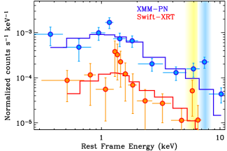
Figure 9.— X-ray spectra of SN 2009ip. The Swift-XRT spectrum collects observations obtained around the optical peak ($t_{\rm{pk}}-2$ days until $t_{\rm{pk}}+13$ days, total exposure time of 86 ks). The XMM EPIC-PN spectrum was obtained on 2012 November 3 ($t_{\rm{pk}}+31$ days, total exposure of 55 ks). The spectral model consists of absorbed bremsstrahlung emission at $kT=60$ keV and intrinsic absorption ($\rm{NH_{int}}=0.10^{+0.06}_{-0.05}\times 10^{22}\rm{cm^{-2}}$ and $\rm{NH_{int}}<3.1\times 10^{21}\rm{cm^{-2}}$ for the XMM and XRT spectra, respectively). Contamination by a nearby source lying $\approx 6^{\prime\prime}$ from SN 2009ip is expected for the XMM spectrum. The color-coded shaded areas highlight the presence of possible emission excess with respect to the model.

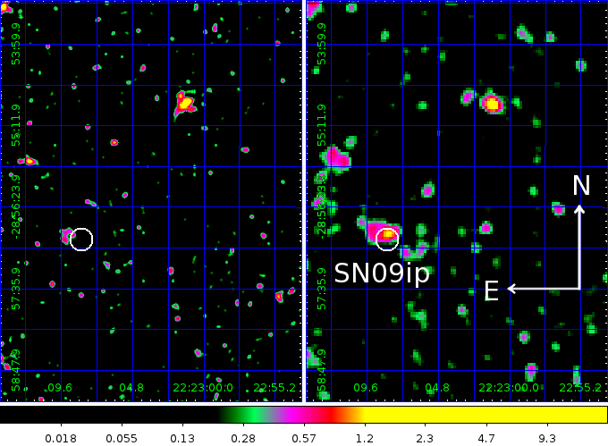
Figure 10.— Left panel: Swift-XRT image of the field of SN 2009ip collecting data before and after the optical peak ($-32\,\rm{days}<t-t_{\rm{pk}}<-2\,\rm{days}$ and $+29\,\rm{days}<t-t_{\rm{pk}}<+83\,\rm{days}$), for a total exposure time of 110 ks. Right panel: same field imaged around the optical peak ($-2\,\rm{days}<t-t_{\rm{pk}}<+13\,\rm{days}$) for a total exposure of 86 ks. In both panels a white circle marks a $10^{\prime\prime}$ region around SN 2009ip. An X-ray source is detected at a position consistent with SN 2009ip around the optical peak (right panel) with significance of $6.1\sigma$. The contaminating source discussed in the text is apparent in the left image.

We observed SN 2009ip with the Swift/X-Ray Telescope (XRT, Burrows et al. 2005) from 2012 September 4 (20:36:23) until 2013 January 1 (13:43:55), for a total exposure of $260$ ks, covering the time period $-29\,\rm{days}<t-t_{\rm{pk}}<+90\,\rm{days}$. Data have been entirely acquired in Photon Counting (PC) mode and analyzed using the latest HEASOFT (v6.12) release, with standard filtering and screening criteria. No X-ray source is detected at the position of SN 2009ip during the decay of the 2012a outburst ($t<-11$ days), down to a 3$\sigma$ limit of $3\times 10^{-3}\rm{cps}$ in the 0.3-10 keV energy band (total exposure of 12.2 ks). Observations sampling the rise time of the 2012b explosion ( $-11\,\rm{days}<t-t_{\rm{pk}}<-2\,\rm{days}$ ) also show no detection. With 31.4 ks of total exposure the 0.3-10 keV count-rate limit at the SN position is $<1.1\times 10^{-3}\rm{cps}$. Correcting for PSF (Point Spread Function) losses and vignetting and merging the two time intervals we find no evidence for X-ray emission originating from SN 2009ip in the time interval $-29\,\rm{days}<t-t_{\rm{pk}}<-2\,\rm{days}$ down to a limit of $<5.6\times 10^{-4}\rm{cps}$ (0.3-10 keV, exposure time of 43.6 ks). X-ray emission is detected at a position consistent with SN 2009ip starting from $t_{\rm{pk}}-2$ days, when the 2012b explosion approached its peak luminosity in the UV/optical bands (Fig. 8). The source is detected at the level of 5$\sigma$ and $4\sigma$ in the time intervals $-2\,\rm{days}<t-t_{\rm{pk}}<+3\,\rm{days}$ and $+4\,\rm{days}<t-t_{\rm{pk}}<+13\,\rm{days}$, respectively, with PSF and vignetting corrected count-rates of $(1.6\pm 0.3)\times 10^{-3}\rm{cps}$ and $(6.8\pm 1.8)\times 10^{-4}\rm{cps}$ (0.3-10 keV, exposure time of 42 and 44 ks).

Starting from $t_{\rm{pk}}+17$ days, the source is no longer detected by XRT. We therefore activated our XMM-Newton program (PI P. Chandra) to follow the fading of the source. We carried out XMM-Newton observations starting from 2012 November 3 at 13:25:33 ($t_{\rm{pk}}+31$ days). Observations have been obtained with the EPIC-PN and EPIC-MOS cameras in full frame with thin filter mode. The total exposures for the EPIC-MOS1 and EPIC-MOS2 are 62.62 ks and 62.64 ks, respectively, and for the EPIC-PN, the exposure time is 54.82 ks. A point-like source is detected at the position of SN 2009ip with significance of 4.5 $\sigma$ (for EPIC-PN), and rate of $(2.7\pm 0.3)\times 10^{-3}$ cps in a region of $10^{\prime\prime}$ around the optical position of SN 2009ip.

From January until April 2013 the source was Sun constrained for Swift. 10 ks of Swift-XRT data obtained on 2013 April 4.5 ($t_{\rm{pk}}+183$ days, when SN 2009ip became observable again) showed no detectable X-ray emission at the position of the transient down to a 3$\sigma$ limit of $4.1\times 10^{-3}$ cps (0.3-10 keV).

We use the EPIC-PN observation to constrain the spectral parameters of the source. We extract photons from a region of $10^{\prime\prime}$ radius to avoid contamination from a nearby source (Fig. 10). The XMM-Newton software SAS is used to extract the spectrum. Our spectrum contains a total of 132 photons. We model the spectrum with an absorption component (which combines the contribution from the Galaxy and from SN 2009ip local environment, $tbabs\times ztbabs$ within Xspec) and an emission component. Both thermal bremsstrahlung and thermal emission from an optically thin plasma in collisional equilibrium (Xspec MEKAL model) can adequately fit the observed spectrum. In both cases we find $kT>10$ keV and intrinsic hydrogen absorption of $\rm{NH_{int}}\approx 10^{21}\,\rm{cm^{-2}}$. In the following we assume thermal bremsstrahlung emission with $kT=60$ keV (this is the typical energy of photons expected from shock break-out from a dense CSM shell, see Section 7.5). The Galactic absorption in the direction of SN 2009ip is $N_{\rm H,MW}=1.2\times 10^{20}$ cm^-2 (Kalberla et al., 2005). The best-fitting neutral hydrogen intrinsic absorption is constrained to be $\rm{NH_{int}}=0.10^{+0.06}_{-0.05}\times 10^{22}\rm{cm^{-2}}$. Using these parameters, the corresponding unabsorbed (absorbed) flux is $(1.9\pm 0.2)\times 10^{-14}\rm{erg\,s^{-1}cm^{-2}}$ ($(1.7\pm 0.2)\times 10^{-14}\rm{erg\,s^{-1}cm^{-2}}$) in the $0.3-10$ keV band. The spectrum is displayed in Fig. 9 and shows some evidence for an excess of emission around $\sim 7-8$ keV (rest-frame) which might be linked to the presence of Ni or Fe emission lines (see e.g. SN2006jd and SN2010jl; Chandra et al. 2012a, b).

A Swift-XRT spectrum extracted around the peak ($-2\,\rm{days}<t-t_{\rm{pk}}<+13\,\rm{days}$, total exposure of 86 ks) can be fit by a thermal bremsstrahlung model, assuming $kT=60$ keV and $\rm{NH_{int}}<3.1\times 10^{21}\rm{cm^{-2}}$ at the $3\sigma$ c.l. As for XMM, we use a $10^{\prime\prime}$ extraction region to avoid contamination from a nearby source (Fig. 10). The count-to flux conversion factor deduced from this spectrum is $3.8\times 10^{-11}\rm{erg\,s^{-1}cm^{-2}ct^{-1}}$ (0.3-10 keV, unabsorbed). We use this factor to calibrate our Swift-XRT light-curve. The complete X-ray light-curve is shown in Fig. 8.

We note that at the resolution of XMM and Swift-XRT we cannot exclude the presence of contaminating X-ray sources at a distance $\lesssim 10^{\prime\prime}$. We further investigate this issue constraining the level of the contaminating flux by merging the Swift-XRT time intervals that yielded a non-detection at the SN 2009ip position. Using data collected between $t_{\rm{pk}}-29$ days and $t_{\rm{pk}}-2$ days, complemented by observations taken between $t_{\rm{pk}}+29$ days and $t_{\rm{pk}}+90$ days, we find evidence for an X-ray source located at RA=22^h23^m09.19^s and Dec=$-$28^∘56^′48.7^′′ (J2000), with an uncertainty of $3.8^{\prime\prime}$ radius ($90\%$ containment), corresponding to $1^{\prime\prime}$ from SN 2009ip. The source is detected at the level of $3.4\sigma$ with a PSF, vignetting and exposure corrected count-rate of $(3.0\pm 0.9)\times 10^{-4}$ cps (total exposure of 110 ks, 0.3-10 keV energy band). The field is represented in Fig. 10, left panel. This source contaminates the reported SN 2009ip flux at the level of $\sim 1.6\times 10^{-4}$ cps. Adopting the count-to-flux conversion factor above, this translates into a contaminating unabsorbed flux of $\sim 6\times 10^{-15}\rm{erg\,s^{-1}cm^{-2}}$ (luminosity of $\sim 5\times 10^{38}\rm{erg\,s^{-1}}$ at the distance of SN 2009ip), representing $\sim 10\%$ the X-ray luminosity of SN 2009ip at peak. This source does not dominate the X-ray energy release around the peak time.

Observations obtained with the Chandra X-ray Observatory (PI D. Pooley) on $t_{\rm{pk}}+19$ days reveal the presence of an additional X-ray source lying $\approx 6"$ from SN 2009ip and brighter than SN 2009ip at that time. SN 2009ip is also detected (Pooley, private communication). Our contemporaneous Swift-XRT observations constrain the luminosity of the contaminating source to be $\lesssim 1.5\times 10^{39}\rm{erg\,s^{-1}}$, $\lesssim 30\%$ the X-ray luminosity of SN 2009ip at peak. We conclude that the contaminating source is not dominating the X-ray emission of SN 2009ip around peak, if stable. The temporal coincidence of the peaks of the X-ray and optical emission of SN 2009ip is suggestive that the detected X-ray emission is physically associated with SN 2009ip. However, given the uncertain contamination, in the following we conservatively assume $L_{\rm{x}}\lesssim 2.5\times 10^{39}\rm{erg\,s^{-1}}$ for the peak X-ray luminosity of SN 2009ip.

2.9. Hard X-ray observations: Swift-BAT

Stellar explosions embedded in an optically thick medium have been shown to produce a collisionless shock when the shock breaks out from the progenitor environment, generating photons with a typical energy $\gtrsim 60$ keV (Murase et al. 2011, Katz et al. 2011). We constrain the hard X-ray emission from SN 2009ip exploiting our Swift-BAT (Burst Alert Telescope, Barthelmy et al. 2005) campaign with observations obtained between 2012 September 4 ($t_{\rm{pk}}-29$ days) and 2013 January 1 ($t_{\rm{pk}}+90$ days) in survey mode (15-150 keV energy range). We analyzed the Swift-BAT survey data following standard procedures: sky images and source rates were obtained by processing the data with the batsurvey tool adopting standard screening and weighting based on the position of SN 2009ip. Following the BAT survey mode guidelines, fluxes were derived in the four standard energy channels, 14–24, 24–50, 50–100, and 100–195 keV. We converted the source rates to energy fluxes assuming a typical conversion factor of $(5.9\pm 1.0)\times 10^{-7}$ erg cm^-2 s^-1/count s^-1, estimated assuming a range of different photon indices of a power–law spectrum ($\Gamma=1-3$). In particular, analyzing the data acquired around the optical peak we find evidence for a marginal detection at the level of $3.5\sigma$ in the time interval $-0.8\,\rm{days}<t-t_{\rm{pk}}<+0.2\,\rm{days}$ (corresponding to 2012 October 2.2 – 3.2). A spectrum extracted in this time interval can be fit by a power–law spectrum with photon index $\Gamma=1.8\pm 1.0$ (90% c.l.) leading to a flux of $(2.6\pm 1.4)\times 10^{-10}\rm{erg\,s^{-1}cm^{-2}}$ (90% c.l., 15-150 keV, total exposure time of $7.0$ ks). The simultaneity of the hard X-ray emission with the optical peak is intriguing. However, given the limited significance of the detection and the known presence of a non-Gaussian tail in the BAT noise fluctuations (H. Krimm, private communication), we conservatively use $F<7\times 10^{-10}\rm{erg\,s^{-1}cm^{-2}}$ ($L<8\times 10^{40}\rm{erg\,s^{-1}}$) as the $5\sigma$ upper limit to the hard X-ray emission from SN 2009ip around maximum light, as derived from the spectrum above.

2.10. GeV observations: Fermi-LAT

GeV photons are expected to arise when the SN shock collides with a dense circumstellar shell of material, almost simultaneous with the optical light-curve peak (Murase et al. 2011, Katz et al. 2011). We searched for high-energy $\gamma$-ray emission from SN 2009ip using all-sky survey data from the Fermi Large Area Telescope (LAT; Atwood et al., 2009), starting from 2012 September 3 ($t_{\rm{pk}}-30$ days) until 2012 October 31 ($t_{\rm{pk}}+28$ days). We use events between 100 MeV and 10 GeV from the P7SOURCE_V6 data class (Ackermann et al., 2012), which is well suited for point-source analysis. Contamination from $\gamma$-rays produced by cosmic-ray interactions with the Earth’s atmosphere is reduced by selecting events arriving at LAT within 100°  of the zenith. Each interval is analyzed using a Region Of Interest (ROI) of 12°  radius centered on the position of the source. In each time window, we performed a spectral analysis using the unbinned maximum likelihood algorithm gtlike. The background is modeled with two templates for diffuse $\gamma$-ray background emission: a Galactic component produced by the interaction of cosmic rays with the gas and interstellar radiation fields of the Milky Way, and an isotropic component that includes both the contribution of the extragalactic diffuse emission and the residual charged-particle backgrounds. We fix the normalization of the Galactic component but leave the normalization of the isotropic background as a free parameter. We also include the bright source 2FGL J2158.8$-$3013, located at approximately $5\fdg 48$ from the location of SN 2009ip, and we fixed its parameters according to the values reported in Nolan et al. (2012).

We find no significant emission at the position of SN 2009ip. Assuming a simple power-law spectrum with photon index $\Gamma=2$, the typical flux upper limits in 1-day intervals are $\lesssim(1-3)\times 10^{-10}$ ergs cm^-2 s^-1 (100 MeV – 10 GeV energy range, 95% c.l.). Integrating around the time of the optical peak ($-2\,\rm{days}<t-t_{\rm{pk}}<+4\,\rm{days}$ ) we find $F<[2.1,1.9,3.6]\times 10^{-11}$ ergs cm^-2 s^-1 for three energy bands (100 MeV–464 MeV, 464 MeV–2.1 GeV and 2.1 GeV–10 GeV).

3. Evolution of the continuum from the UV to the NIR

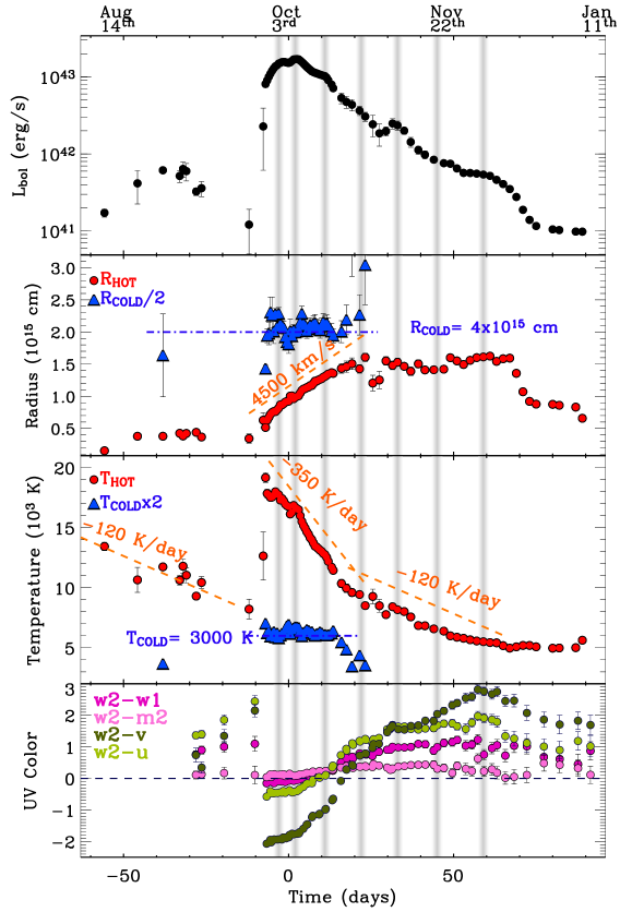
Figure 11.— Upper panel: Bolometric light-curve of SN 2009ip calculated from the best-fitting black-body temperatures and radii displayed in the intermediate panels. Lower panel: UV color evolution with time. The onset of the 2012b explosion corresponds to a sudden change in UV colors. After that, the UV colors become progressively redder. In this plot, v and u refers to the optical photometry in the UVOT system. Vertical shaded bands mark the time of observed bumps in the photometry of Fig. 2: some are powerful enough to be clearly visible in the bolometric luminosity curve as well.

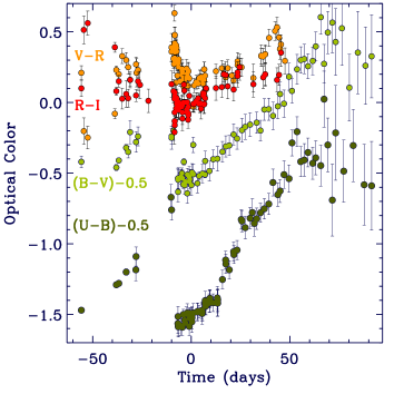
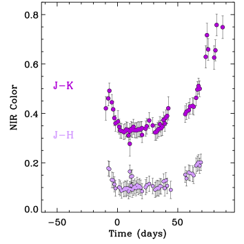
Figure 12.— Upper panel: Optical colors. UVOT magnitudes have been converted into the Johnson filters using a dynamical correction that accounts for the evolution of the color of the source. Lower panel: NIR colors. While SN 2009ip clearly evolves towards redder optical colors starting from $t_{\rm{pk}}-3$ days, no strong evolution is apparent in the NIR colors in the same time interval.

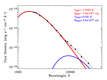
Figure 13.— Black solid line: best fitting SED model obtained at $t_{\rm{pk}}-4.5$ days which clearly shows the presence of the ”hot” (red line) and ”cold” (blue line) components in the spectrum.

Our 13-filter photometry allows us to constrain the evolution of the spectral energy distribution (SED) of SN 2009ip with high accuracy. We fit a total of 84 SEDs, using data spanning from the UV to the NIR.

The extremely blue colors and color evolution of SN 2009ip (see Fig. 11, lower panel, and Fig. 12) impose non-negligible deviations from the standard UVOT count-to-flux conversion factors. The filter passbands (e.g. the presence of the ”red leak” in the w2 and w1 filters) also affects the energy distribution of the detected photons for different incoming spectra. Because of the rapidly changing spectral shape in the UV, even the ratio of intrinsic flux to observed counts through the m2 filter, which has no significant red leak, is strongly dependent on the spectral shape. We account for these effects as follows: first, for each filter, we determine a grid of count-to-flux conversion factors at the effective UVOT filters Vega wavelengths listed in Poole et al. 2008, following the prescriptions by Brown et al. (2010). We assume a black-body spectrum as indicated by our analysis of the SED of SN 2009ip at optical wavelengths. Our grid spans the temperature range between 2000 K and 38000 K with intervals of 200 K. We observe a variation in the conversion factor of $90\%$, $17\%$, $7\%$ and $5\%$ in the w2, m2 , w1 and u filters as the temperature goes from 6000 K to 20000 K. For the v and b filters the variation is below $1\%$. As a second step we iteratively fit each SED consisting of UVOT plus ground-based observations until the input black-body temperature assumed to calibrate the UVOT filters matches the best-fitting temperature within uncertainties.

For $t>t_{\rm{pk}}-7$ days the UV+BVRI SED is well fitted by a black-body spectrum with a progressively larger radius (”hot” black-body component in Fig. 11). The temperature evolution tracks the bolometric luminosity, with the photosphere becoming appreciably hotter in correspondence with light-curve bumps and then cooling down after the peak occurred. Around $t_{\rm{pk}}+70$ days the temperature settles to a floor around $5000$ K and remains nearly constant in the following 20 days. The temperature has been observed to plateau at similar times in some SNe IIn (e.g. SN 2005gj and SN 1998S where the black-body temperature reached a floor at $\sim 6000-6500$ K; Prieto et al. 2007, Fassia et al. 2000) and in SNe IIP as well (e.g. SN 1999em, with a plateau at $\sim 5000$ K; Leonard et al. 2002).

The black body radius increases from $\sim 5.1\times 10^{14}\,\rm{cm}$ to $\sim 6.3\times 10^{14}\rm{cm}$ in $\sim 0.3$ days (from $t=t_{\rm{pk}}-6.8$ days to $t=t_{\rm{pk}}-6.5$ days), then makes a transition to a linear evolution with average velocity of $\sim 4000-4500\,\rm{km\,s^{-1}}$ until $t_{\rm{pk}}+20$ days, followed by a plateau around $R_{\rm{HOT}}=1.6\times 10^{15}\rm{cm}$. In the context of the interaction scenario of Section 8 this change in the black-body radius evolution with time likely marks the transition to when the interaction shell starts to become optically thin (the black-body radius is a measure of the effective radius of emission: the shock radius obviously keeps increasing with time). A rapid decrease in radius is observed around $t_{\rm{pk}}+70$ days. After this time the $R_{\rm{HOT}}$ mimics the temporal evolution of the bolometric light-curve (see Fig. 11). In SNe dominated by interaction with pre-existing material, the black-body radius typically increases steadily with time, reaches a peak and then smoothly transitions to a decrease (see e.g. SN 1998S, Fassia et al. 2000; SN 2005gj, Prieto et al. 2007). The more complex behavior we observe for SN 2009ip likely results from a more complex structure of the immediate progenitor environment (Section 8).

Starting from $t_{\rm{pk}}+16$ days, the best-fitting black body model tends to over-predict the observed flux in the UV, an effect likely due to increasing line-blanketing. As the temperature goes below $\sim 10^{4}$ K, the recombination of the ejecta induces a progressive strengthening of metal-line blanketing which is responsible for partially blocking the UV light.We account for line-blanketing by restricting our fits to the UBVRI flux densities for $t>t_{\rm{pk}}+16$ days. Our fits still indicate a rapidly decreasing temperature with time. We conclude that the rapid drop in UV light observed starting from $t_{\rm{pk}}+12$ days mainly results from the cooling of the photosphere.

Starting around $t_{\rm{pk}}+59$ days the UV emission fades more slowly and we observe a change in the evolution of the UV colors: from red to blue (Fig. 11, lower panel). The same evolution is observed in the (U-B) color of Fig. 12. This can also be seen from Fig. 2, where the NIR emission displays a more rapid decay than the UV. This manifests as an excess of UV emission with respect to the black-body fit. After $t_{\rm{pk}}+67$ days a pure black-body spectral shape provides a poor representation of the UV to NIR SED.

We furthermore find clear evidence for excess of NIR emission with respect to the hot black body (see Fig. 13) as we first reported in Gall et al. (2012), based on the analysis of the VLT/X-shooter spectra (Fig. 19 and 20). Modeling the NIR excess with an additional black-body component, we obtain the radius and temperature evolution displayed in Fig. 11 (”cold” black body). The cold black-body radius is consistent with no evolution after $t_{\rm{pk}}-4$ days, with $R_{\rm{COLD}}\sim 4\times 10^{15}\rm{cm}$. $T_{\rm{COLD}}$ is also found to be $T_{\rm{COLD}}\sim 3000$ K until $t_{\rm{pk}}+14$ days, which implies $L_{\rm{COLD}}\approx const$ for $-4\,\rm{days}<t-t_{\rm{pk}}<+14\,\rm{days}$ (together with the almost unchanged NIR colors of Fig. 12). Starting from $t_{\rm{pk}}+16$ days $T_{\rm{COLD}}$ cools down to reach $T_{\rm{COLD}}\sim 2000$ K on $t_{\rm{pk}}+23$ days. At this stage the hot black body with $T_{\rm{HOT}}\sim 8500$ K completely dominates the emission at NIR wavelengths and the fit is no longer able to constrain the parameters of the cold component. Our NIR spectra of Fig. 7 clearly rule out line-emission as a source of the NIR excess.

Applying the same analysis to the 2012a outburst we find that the temperature of the photosphere evolved from $\sim 13400$ K (at $t_{\rm{pk}}-56$ days) to $8000$ K ($t_{\rm{pk}}-12$ days), with an average decay of $\sim 120\,\rm{K/day}$. Our modeling shows a slightly suppressed UV flux which we interpret as originating from metal line-blanketing. Notably, the SED at $t_{\rm{pk}}-38$ days (when we have almost contemporaneous coverage in the UBVRI and JHK bands) shows evidence for a NIR excess corresponding to $T_{\rm{COLD}}\sim 2000$ K at the radius consistent with $R_{\rm{COLD}}\sim 4\times 10^{15}\rm{cm}$ (as found for the NIR excess during the 2012b explosion).

Finally, we use the SED best-fitting models above to compute the bolometric luminosity of SN 2009ip. Displayed in Fig. 11 is the contribution of the ”hot” black body. The ”cold” black-body contribution is marginal, being always $(2-4)\%$ the luminosity of the ”hot” component.

4. Spectral changes at UV/optical/NIR frequencies

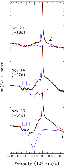
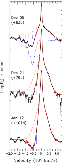
Figure 14.— Evolution of the H$\alpha$ line profile with time. Orange dashed line: emission components. Blue dot-dashed line: absorption components. Red thick line: composite line profile. The vertical blue lines mark the velocity of the absorption components.

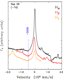
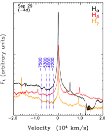
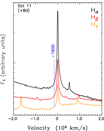
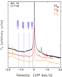
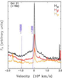
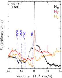
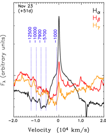
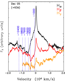
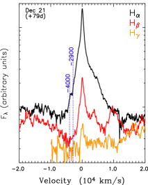
Figure 15.— H$\alpha$, H$\beta$ and $H\gamma$ line profiles of SN 2009ip at representative epochs. The blue dotted lines mark the velocity of the major absorption components identified by our fits of the H$\alpha$ line profile. For 2012 December 5 we also added two absorption components at $-1000\,\rm{km\,s^{-1}}$ and $-4000\,\rm{km\,s^{-1}}$ identified in the H$\beta$ and H$\gamma$ lines. The late-time spectrum acquired on $t_{\rm{pk}}+101$ days (2013 January 12) shows limited evolution in the H$\alpha$ profile with respect to the previous epoch and it is not shown here.

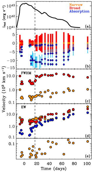
Figure 16.— Evolution of the H$\alpha$ line with time. We model the H$\alpha$ line with a combination of Lorentzian and Gaussian profiles. Orange markers represent the narrow Lorentzian profile. Red is used for the broad component, while blue is associated with the blue-shifted absorption components. Panel (a): bolometric light-curve for reference. Panel (b): the red (orange) bars span the FWHM of the broad (narrow) component. These values are also reported in panel (c). Blue dots: absorption minima as obtained by modeling the absorption with a combination of Gaussians. Negative values indicate blue-shifted components. We use light-blue bars to mark the $1\sigma$ width as obtained from the fit. Panel (d) shows the evolution of the equivalent width of the narrow (orange), broad (red) and absorption (blue) components. The peak of the narrow component progressively shifts to larger redshifted velocities as illustrated in Panel (e) and independently found by Fraser et al. (2013). The vertical dashed line marks an important time in the evolution of SN 2009ip from different perspectives: from this plot it is clear that around this time the width of broad component undergoes a remarkable transition from FWHM$\sim 3000\,\rm{km\,s^{-1}}$ to FWHM$\sim 10000\,\rm{km\,s^{-1}}$.

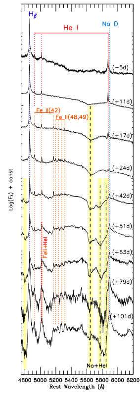
Figure 17.— Key spectral changes in SN 2009ip between 4500$-$6200 Å: narrow He I emission lines subside while Na I D emission grows in strength. He I later re-appears with the broad/intermediate component. Fe II emission lines emerge, while broad absorption dips develop red-wards the Na I D (and He I) lines, around 5650 Å. Starting from $\sim t_{\rm{pk}}+30$ days, additional broad absorption features around 5770 Å  and 5850 Å  appear, associated with the He I and the Na I D lines; H I lines develop strong absorption on their blue wing.

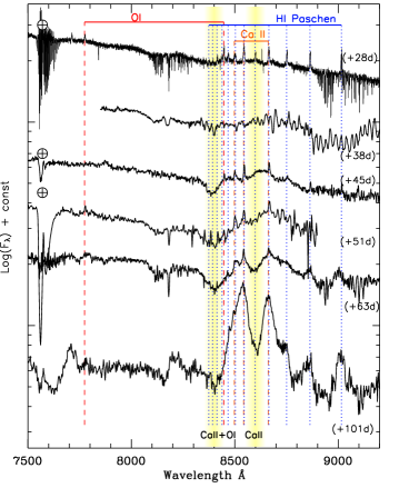
Figure 18.— Beginning at $t_{\rm{pk}}+30$ days SN 2009ip develops broad emission and absorption components between 8300 Å  and 9000 Å  we attribute to Ca II. NIR emission from the CaII triplet is typical of IIP SNe (e.g. Pastorello et al. 2006).

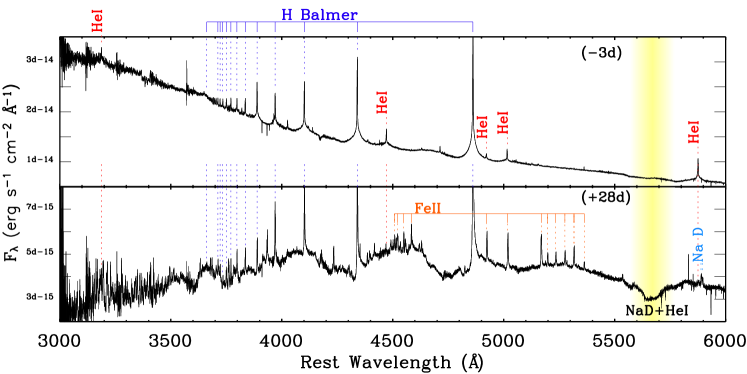
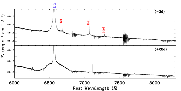
Figure 19.— High-resolution VLT/X-shooter spectra captured the evolution of SN 2009ip in fine detail. Upper panel: around the optical peak, on 2012 September 30 ($t_{\rm{pk}}-3$ days), SN 2009ip shows a narrow-line dominated spectrum typical of SNe (and LBVs) interacting with a medium. One month later (lower panel of each plot) SN 2009ip started to develop broad emission components (see in particular the H$\alpha$ line) and deep absorption features (e.g. the yellow-shaded band around $5650\,$Å ) more typical of SNe IIP. The complementary $10000-24500$ Å  wavelength range is shown in Fig. 20. Data have been corrected for Galactic extinction.

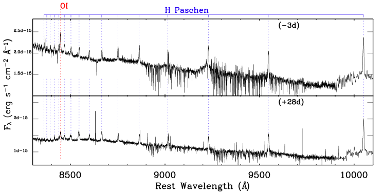
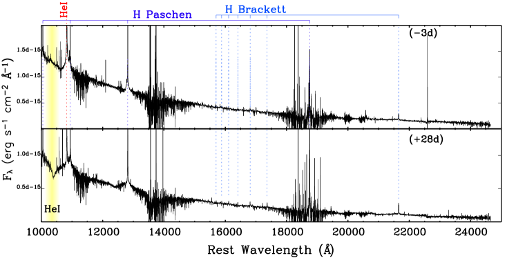
Figure 20.— High-resolution VLT/X-shooter spectra from $10000$ to $24500$ Å . Continued from Fig. 19.

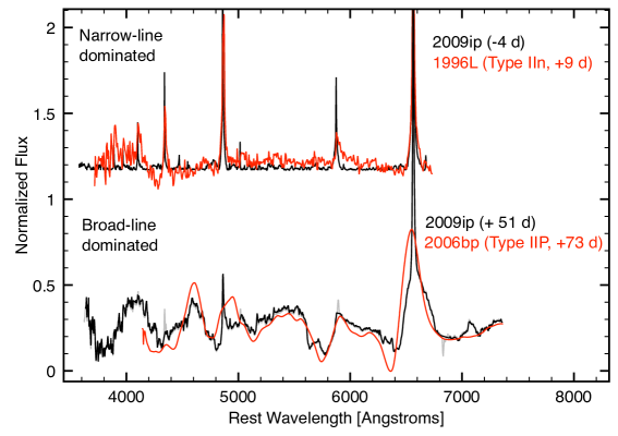
Figure 21.— SN 2009ip evolved from a narrow-line dominated spectrum typical of Type IIn SN explosions to a spectrum that clearly shows broad absorption features more typical of Type IIP SNe. Here we show the spectrum of Type IIn SN 1996L (Benetti et al., 1999) and Type IIP SN 2006bp (Quimby et al., 2007).

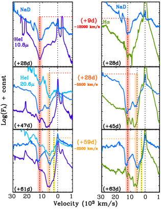
Figure 22.— Evolution of the broad absorption features associated with H$\alpha$, He I and Na I D lines. As the photosphere recedes into the ejecta broad absorption features appear in the spectra with 3 typical velocities: $v\sim-12000\,\rm{km\,s^{-1}}$ (red band); $v\sim-5500\,\rm{km\,s^{-1}}$ (orange band) and $v\sim-2500\,\rm{km\,s^{-1}}$ (yellow band). Absorption features at higher velocity are revealed at earlier times: we clearly detect material with $v\sim-12000\,\rm{km\,s^{-1}}$ starting around $t_{\rm{pk}}+9$ days; material with $v\sim-5500\,\rm{km\,s^{-1}}$ starts to be detected around $t_{\rm{pk}}+28$ days, while slowly moving ejecta with $v\sim-2500\,\rm{km\,s^{-1}}$ is only detected $\sim 60$ days after peak. Left panel: velocity profile of the absorption arising from Na I D plus He I ($\lambda=5876$ Å), compared with HeI $1.08\,\mu\rm{m}$ and HeI $2.06\,\mu\rm{m}$ velocity profiles. Right panel: Na I D plus He I ($\lambda=5876$ Å) vs. H$\alpha$ velocity profile.

Pastorello et al. (2012) find the spectrum of SN 2009ip during the 2012a outburst to be dominated by prominent Balmer lines. In particular, spectra collected in August and September 2012 show clear evidence for narrow emission components (FWHM$\approx 800\,\rm{km\,s^{-1}}$ for $\rm{H}\alpha$) accompanied by absorption features, indicating the presence of high velocity material with velocities extending to $v\approx-14000\,\rm{km\,s^{-1}}$ (Mauerhan et al. 2013). Our 2012 August 26 spectrum confirms these findings. SN 2009ip experienced a sudden re-brightening around 2012 September 23 ($t_{\rm{pk}}-10$ days, Brimacombe 2012; Margutti et al. 2012), signaling the beginning of the 2012b explosion. By this time the $\rm{H}\alpha$ line developed a prominent broad emission component with FWHM$\approx 8000\,\rm{km\,s^{-1}}$ (Mauerhan et al., 2013, their Fig. 5). The broad component disappeared 3 days later: our spectrum obtained on 2012 September 26 ($t_{\rm{pk}}-7$ days) indicates that the $\rm{H}\alpha$ line evolved back to the narrow profile (Fig. 14), yet still retained evidence for absorption with a core velocity $v\approx-5000\,\rm{km\,s^{-1}}$, possibly extending to $v\approx-7500\,\rm{km\,s^{-1}}$. By 2012 September 30 ($t_{\rm{pk}}-3$ days, Fig. 19 and 20) the spectrum no longer shows evidence for the high velocity components in absorption and is instead dominated by He I and H I lines with narrow profiles.

In the following months SN 2009ip progressively evolves from a typical SN IIn (or LBV-like) spectrum with clear signs of interaction with the medium, to a spectrum dominated by broad absorption features, more typical of SNe IIP (Fig. 21). Our two Xshooter spectra (Fig. 19 and 20) sample two key points in this metamorphosis, providing a broad band view of these spectral changes at high resolution. Broad features completely disappear by the time of our observations in April 2013 ($t_{\rm{pk}}+190$ days, Fig. 31). At no epoch we find evidence for very narrow, low velocity blue shifted absorption at $v\sim-100\,\rm{km\,s^{-1}}$, differently from what typically observed in Type IIn SNe and LBVs (see e.g. SN 2010jl, Smith et al. 2012). The major spectral changes during the 2012b explosion can be summarized as follows:

• Broad/intermediate absorption/emission features progressively re-appear in the H Balmer lines, with evidence of multiple velocity components (Fig. 14, 15 and 16).

• Narrow He I lines weaken with time (Fig. 17); He I later re-emerges with the intermediate component only.

• Fe II features re-emerge and later develop P Cygni profiles.

• Emission originating from Na I D is detected (Fig. 17).

• A broad near-infrared Ca II triplet feature typical of Type IIP SNe develops starting around 2012 November 15 (Fig. 18).

• More importantly, SN 2009ip progressively develops broad absorption dips which have never been observed in LBV-like eruptions, while being typical of a variety of SN explosions (Fig. 17). Broad absorption dips disappear $\sim 200$ days after peak.

Around $100$ days after peak, emission from forbidden transitions (see e.g. [CaII] $\lambda\lambda$ 7291, 7324 in Fig. 6) starts to emerge. At this time SN 2009ip settles behind the Sun. Despite limited spectral evolution between $t_{\rm{pk}}+100$ days and $t_{\rm{pk}}+200$ days (when SN 2009ip re-emerges from the Sun constraint) we do observe the absorption features to migrate to lower velocities. We discuss each of the items below.

Additional optical/NIR spectroscopy of SN 2009ip during the 2012b explosion has been published by Mauerhan et al. (2013), Pastorello et al. (2012), Levesque et al. (2012), Smith et al. (2013) and Fraser et al. (2013): we refer to these works for a complementary description of the spectral changes underwent by SN 2009ip.

4.1. Evolution of the H I line profiles

The H$\alpha$ line profile experienced a dramatic change in morphology after the source suddenly re-brightened on 2012 September 23. Figure 14 shows the H$\alpha$ line at representative epochs: at any epoch the H$\alpha$ line has a complex profile resulting from the combination of a narrow (Lorentzian) component (FWHM$<1000\,\rm{km\,s^{-1}}$), intermediate/broad width components (FWHM$>1000\,\rm{km\,s^{-1}}$) and blue absorption features with evidence for clearly distinguished velocity components. Emission and absorption components with similar velocity are also found in the H$\beta$ and H$\gamma$ line profiles (Fig. 15).

The evolution of the line profile results from changes in the relative strengths of the different components in addition to the appearance (or disappearance) of high-velocity blue absorption edges. The evolution of the width and relative strength of the different components is schematically represented in Fig. 16. The broad component dominates over the narrow emission starting from $t_{\rm{pk}}+33$ days and reaches its maximum width at $t_{\rm{pk}}+51$ days. After this time, the width of the broad component decreases. There is evidence for an increasing width of the narrow component with time, accompanied by a progressive shift of the peak to higher velocities. Finally, high-velocity ($v>1000\,\rm{km\,s^{-1}}$) absorption features get stronger as the light-curve makes the transition from the rise to the decay phase. The spectral changes are detailed below.

By $t_{\rm{pk}}-7$ days the broad components dominating the line profile 10 days before (Mauerhan et al. 2013) have weakened to the level that most of the emission originates from a much narrower component which is well described by a Lorentzian profile with FWHM$\approx 1000\,\rm{km\,s^{-1}}$. Absorption from high velocity material ($v\approx-5000\,\rm{km\,s^{-1}}$, measured at the minimum of the absorption feature) is still detected when the 2012b explosion luminosity is still rising. The high-resolution spectra collected on $t_{\rm{pk}}-5$ and $t_{\rm{pk}}-4$ days allow us to resolve different blue absorption components: modeling these absorption features with Gaussians, the central velocities are found to be $v\approx-2200\,\rm{km\,s^{-1}}$, $\approx-4000\,\rm{km\,s^{-1}}$, $\approx-5300\,\rm{km\,s^{-1}}$, $\approx-7500\,\rm{km\,s^{-1}}$ with $\sigma\approx 300-500\,\rm{km\,s^{-1}}$. These absorption features are detected in the $H\beta$ and $H\gamma$ lines as well (Fig. 15). The width of the narrow component of emission decreases to FWHM$\approx 280\,\rm{km\,s^{-1}}$.

On 2012 September 30 ($t_{\rm{pk}}-3$ days) SN 2009ip approaches its maximum luminosity (Fig. 11). From our high-resolution spectrum the H$\alpha$ line is well modeled by the combination of two Lorenztian profiles with FWHM$\approx 240\,\rm{km\,s^{-1}}$ and FWHM$\approx 2600\,\rm{km\,s^{-1}}$. We find no clear evidence for absorption components. Interpreting the broad wings as a result of multiple Thomson scattering in the circumstellar shell of the narrow-line radiation (Chugai, 2001) suggests that the optical depth of the unaccelerated circumstellar shell envelope to Thomson scattering is $\tau\sim 3$.

High-velocity absorption features in the blue wing of the H$\alpha$ line progressively re-appear as the luminosity of the explosion enters its declining phase. Eight days after peak the H$\alpha$ line exhibits a combination of narrow (FWHM$\approx 340\,\rm{km\,s^{-1}}$) and broad (FWHM$\approx 2000-3000\,\rm{km\,s^{-1}}$) Lorentzian profiles and a weak P Cygni profile with an absorption minimum around $-1600\,\rm{km\,s^{-1}}$. Three days later ($t_{\rm{pk}}+11$ days) the broad component (FWHM$\approx 2600\,\rm{km\,s^{-1}}$) of emission becomes more prominent while the width of the narrow Lorentzian profile decreases again to FWHM$\approx 220\,\rm{km\,s^{-1}}$. At this time the bolometric light-curve exhibits a third bump (Fig. 11). High-velocity absorption features re-appear in the blue wing of the H$\alpha$ line with absorption minima at $v\approx-12000\,\rm{km\,s^{-1}}$ and $v\approx-8000\,\rm{km\,s^{-1}}$ ($\sigma\sim 1000\,\rm{km\,s^{-1}}$). The low velocity P Cygni absorption is also detected at $v\approx-1200\,\rm{km\,s^{-1}}$. The $H\beta$ and $H\gamma$ lines possibly show evidence for an additional absorption edge at $v\approx-4000\,\rm{km\,s^{-1}}$ (Fig. 15).

A lower resolution spectrum obtained on $t_{\rm{pk}}+18$ days shows the development of an even stronger broad emission component with FWHM$\approx 9400\,\rm{km\,s^{-1}}$. While we cannot resolve the different components of velocity responsible for the blue absorption, we find clear evidence for a deep minimum at $v\approx-10000\,\rm{km\,s^{-1}}$ with edges extending to $v\approx-14000-15000\,\rm{km\,s^{-1}}$. The broad emission component keeps growing with time: at $t_{\rm{pk}}+42$ days it clearly dominates the H$\alpha$ profile. At this epoch the H$\alpha$ line consists of a narrow component with FWHM$\approx 240\,\rm{km\,s^{-1}}$, a broad emission component (FWHM$\approx 10600\,\rm{km\,s^{-1}}$) and a series of absorption features on the blue wing (both at high and low velocity). Our high-resolution spectrum resolve the absorption minima at $v\approx-12500\,\rm{km\,s^{-1}}$, $\approx-10000\,\rm{km\,s^{-1}}$, $\approx-7000\,\rm{km\,s^{-1}}$ and $\approx-1300\,\rm{km\,s^{-1}}$ (Fig. 14). The $H\beta$ and $H\gamma$ lines exhibit an additional blue absorption at $v\approx 3000\,\rm{km\,s^{-1}}$ (Fig. 15).

By $t_{\rm{pk}}+51$ days the broad component which dominates the H$\alpha$ line reaches FWHM$\approx 13600\,\rm{km\,s^{-1}}$. High velocity absorption features are still detected at $v\approx-12500\,\rm{km\,s^{-1}}$ and $\approx-10000\,\rm{km\,s^{-1}}$. The absorption feature at $v\approx-7000\,\rm{km\,s^{-1}}$ becomes considerably more pronounced and shows clear evidence for two velocity components with minima at $v\approx-7900\,\rm{km\,s^{-1}}$ and $v\approx-5700\,\rm{km\,s^{-1}}$. The low-velocity absorbing component is also detected with a minimum at $v\approx-1000\,\rm{km\,s^{-1}}$. A spectrum obtained 63 days after maximum shows little evolution in the H$\alpha$ profile, the only difference being a more pronounced absorption at $v\approx-5700\,\rm{km\,s^{-1}}$. At $t_{\rm{pk}}+79$ days we find a less prominent broad component: by this time its width decreased from FWHM$\approx 12500\,\rm{km\,s^{-1}}$ to FWHM$\approx 8200\,\rm{km\,s^{-1}}$. A spectrum obtained at $t_{\rm{pk}}+101$ days confirms this trend (FWHM of the broad component $\approx 7500\,\rm{km\,s^{-1}}$): the bulk of the absorption is now at lower velocities $v\approx-3100\,\rm{km\,s^{-1}}$ (with a tail possibly extending to $v\approx-8000\,\rm{km\,s^{-1}}$). At $t_{\rm{pk}}+190$ days the blue-shifted absorption is found peaking at even lower velocities of $v\lesssim-2400\,\rm{km\,s^{-1}}$, and the ”broad” (now intermediate) component has FWHM of only $\approx 2000\,\rm{km\,s^{-1}}$.

Finally, comparing the H Paschen and Brackett emission lines using our two highest resolution spectra collected around the peak (narrow-line emission dominated spectrum at $t_{\rm{pk}}-3$ days) and 28 days after peak (when broad components start to emerge, see Fig. 19 and 20), we find that for both epochs the line profiles are dominated by the narrow component (FWHM$\approx 170\,\rm{km\,s^{-1}}$) with limited evolution between the two. The Paschen $\beta$ line clearly develops an intermediate-broad component starting from $t_{\rm{pk}}+33$ days (see Fig. 7). Spectra obtained by Pastorello et al. (2012) before the sudden re-brightening of 2012 September 23 ($t_{\rm{pk}}-10$ days) show a similar narrow plus broad component structure, with the broad emission dominating the narrow lines between 2012 August 26 and 2012 September 23. As for the H Balmer lines, the broad component completely disappeared as the light-curve approached its maximum.

We conclude by noting that, observationally, $t_{\rm{pk}}+17$ days (i.e. 2012 October 20) marks an important transition in the evolution of SN 2009ip: around this time the broad H$\alpha$ component evolves from FWHM$\sim 3000\,\rm{km\,s^{-1}}$ to FWHM$\sim 10000\,\rm{km\,s^{-1}}$ (Fig. 16); the photospheric radius $R_{\rm{HOT}}$ flattens to $R_{\rm{HOT}}\sim 1.6\times 10^{15}\rm{cm}$ while the hot black-body temperature transitions to a milder decay in time (Section 3, Fig. 11). It is intriguing to note that our modeling described in Section 7 independently suggests that this is roughly the time when the explosion shock reaches the edge of the dense shell of material previously ejected by the progenitor.

4.2. The evolution of He I lines

Conspicuous He I lines are not unambiguously detected in our spectrum obtained on 2012 August 26. They are, however, detected in our spectrum acquired one month later, $\sim 3$ days after SN 2009ip re-brightened. At this epoch the light curve of SN 2009ip is still rising. Similarly to H Balmer lines, HeI features (the brightest being at 5876 Å , and $7065$ Å) exhibit a combination of a narrow-intermediate profile (FWHM$\approx 1000\,\rm{km\,s^{-1}}$), a weak broad component (FWHM$\approx 5000\,\rm{km\,s^{-1}}$) together with evidence for a P Cygni absorption at velocity $v\approx-5000\,\rm{km\,s^{-1}}$.

As for the H Balmer lines, high-resolution spectroscopy obtained at $t_{\rm{pk}}-5$ and $t_{\rm{pk}}-4$ days shows the appearance of multiple absorption components on the blue wing of the He I $\lambda 5876$ and $\lambda 7065$ lines, with velocities $v\approx-2000\,\rm{km\,s^{-1}}$, $\approx-4800\,\rm{km\,s^{-1}}$ and $\approx-7000\,\rm{km\,s^{-1}}$ measured at the absorption minima (to be compared with Fig. 15). High velocity absorption features disappear by $t_{\rm{pk}}-3$ days: He I $\lambda 5876$ and $\lambda 7065$ show the combination of a narrow plus broader intermediate Lorentzian profiles with FWHM$\approx 2000\,\rm{km\,s^{-1}}$ and FWHM$\approx 240\,\rm{km\,s^{-1}}$, respectively.

Starting from $t_{\rm{pk}}-3$ days, He I features become weaker until He I $\lambda 7065$ is not detected in our high-resolution spectrum acquired at $t_{\rm{pk}}+28$ days (Fig. 19 and Fig. 19). He I later re-appears in our spectra taken in the second half of November ($t>t_{\rm{pk}}+43$ days) showing the broad/intermediate component only (FWHM$\approx 2500\,\rm{km\,s^{-1}}$ as measured at $t_{\rm{pk}}+63$ days). At $t_{\rm{pk}}+79$ days He I $\lambda 7065$ shows an intermediate-broad emission profile with FWHM$\approx 3000\,\rm{km\,s^{-1}}$. A similar value is obtained at $t_{\rm{pk}}+101$ days. Roughly $100$ days later, on 2013 April 11 He I 7065 Å  is clearly detected with considerably narrower emission (FWHM$\approx 1000\,\rm{km\,s^{-1}}$). He I $\lambda 6678$ also re-emerges on the red wing of the H$\alpha$ profile (Fig. 31).

4.3. The evolution of Fe II lines

A number of Fe II lines from different multiplets have been observed during previous SN 2009ip outbursts (both in 2009, 2011 and the 2012a outburst, see Pastorello et al. 2012, their Fig. 5 and 6). The Fe responsible for this emission is therefore pre-existent the 2012 explosion. Fe II is instead not detected in our spectra until $t_{\rm{pk}}+17$ days (Fig. 17). From the Xshooter spectrum acquired at $t_{\rm{pk}}+28$ days we measure the FWHM of the narrow Fe II lines $\lambda 5018$ and $\lambda 5169$ (multiplet 42): FWHM$\approx 240\,\rm{km\,s^{-1}}$. A similar value has been measured by Pastorello et al. (2012) from their 2012 August 18 and September 5 spectra. As a comparison, the FWHM of the narrow (Lorentzian) component of the H$\alpha$ line measured from the same spectrum is $\approx 170\,\rm{km\,s^{-1}}$. By $t_{\rm{pk}}+63$ days the Fe II emission lines develop a P Cygni profile (Fig. 17), with absorption minimum velocity of $v\approx-1000\,\rm{km\,s^{-1}}$, possibly extending to $v\approx-4000\,\rm{km\,s^{-1}}$.

4.4. The NIR Ca II feature

Starting from $\sim 30$ days after peak, our spectra (Fig. 18) show the progressive emergence of broad NIR emission originating from the Ca II triplet $\lambda\lambda 8498$, $8542$, $8662$ (see also Fraser et al. 2013, their Fig. 4). The appearance of this feature is typically observed during the evolution of Type II SN explosions (see e.g. Pastorello et al. 2006). Interestingly, no previous outburst of SN 2009ip showed this feature (2012a outburst included, see Pastorello et al. 2012). No broad Ca II triplet feature has ever been observed in an LBV-like eruption.

Figure 18 also sjows the emergence of broad absorption dips around 8400 Å  and 8600 Å. If Ca II $\lambda 8662$ is causing the absorption around 8600 Å, the corresponding velocity at the absorption minimum is $v\approx-2400\,\rm{km\,s^{-1}}$. This absorption developed between 51 days and 63 days after peak. The absorption at $\lambda\approx 8400$ Å  is instead clearly detected in our spectra starting from $t_{\rm{pk}}+45$ days and likely results from the combination of OI and CaII. If OI (8447 Å) is dominating the absorption at minimum, the corresponding velocity is $v\approx-1500\,\rm{km\,s^{-1}}$.

4.5. The development of broad absorption features

High-velocity, broad absorption features appear in our spectra starting 9 days after peak (see yellow bands in Fig. 7, Fig. 17, Fig. 19, Fig. 20). Absorption features of similar strength and velocity have never been associated with an LBV-like eruption to date, and are more typical of SNe (Fig. 21). These absorption features are unique to the 2012b explosion and have not been observed during the previous outbursts of SN 2009ip (see Smith et al. 2010b, Foley et al. 2011, Pastorello et al. 2012).

As the photosphere recedes into the ejecta it illuminates material moving towards the observer with different velocities. Our observations identify He I, Na I D and H I absorbing at 3 typical velocities (Fig. 22). The blue absorption edge of He I plus Na I D extends to $v\approx 18000\,\rm{km\,s^{-1}}$, as noted by Mauerhan et al. (2013). High-velocity $v\sim-12000\,\rm{km\,s^{-1}}$ absorption appears first, around $t_{\rm{pk}}+9$ days followed by the $v\sim-5500\,\rm{km\,s^{-1}}$ absorption around $t_{\rm{pk}}+28$ days, which in turn is followed by slower material with $v\sim-2500\,\rm{km\,s^{-1}}$, seen in absorption only starting from $\sim t_{\rm{pk}}+60$ days. This happens since material with lower velocity naturally overtakes the photosphere at later times. Material moving at three distinct velocities argues against a continuous distribution in velocity of the ejecta and suggests instead the presence of distinct shells of ejecta expanding with typical velocity $v\sim-12000\,\rm{km\,s^{-1}}$, $v\sim-5500\,\rm{km\,s^{-1}}$ and $v\sim-2500\,\rm{km\,s^{-1}}$.

4.6. UV spectral properties

Our Swift-UVOT low-resolution spectroscopic monitoring campaign maps the evolution of SN 2009ip during the first month after its major peak in 2012 (Fig. 3). We do not find evidence for strong spectral evolution at UV wavelengths (Fig. 4): as time proceeds the Fe III absorption features become weaker while Fe II develops stronger absorption features, consistent with the progressive decrease of the black-body temperature with time (Fig. 11). UVOT spectra show the progressive emergence of an emission feature around $2500-3000$ Å  that is later well resolved by HST/STIS as emission from Mg II $\lambda\lambda 2796,2803$ lines as well as Fe II multiplets at $\sim 2550,2630,2880$ Å  (Fig. 5). The Mg II line profiles are similar to the H I line profiles, with a narrow component and broad, blue-shifted absorption features. As for the H I lines, the narrow component originates from the interaction with slowly moving CSM. We further identify strong, narrow emission from N II] at $\lambda\lambda 2140,2143$. Emission from C III] ($\lambda 1909$) and Si III] ($\lambda\lambda 1892,1896$) might also be present, but the noise level does not allow a firm identification.

At shorter wavelengths, the HST/COS spectrum taken 34 days after peak shows a mixture of high and low ionization lines (Fig. 5, lower panel). We identify strong lines of C II ($\lambda\lambda 1334.5,1335.7$), O I ($\lambda\lambda$ 1302.2-1306.0), Si II ($\lambda\lambda$ 1526.7, 1533.5). Of the higher ionization lines one notes C IV ($\lambda\lambda 1548.2,1550.8$) and N V ($\lambda\lambda 1238.8,1242.8$). Interestingly, N IV] $\lambda 1486.5$ is either very weak or absent which indicates a medium with density $n\gtrsim 10^{9}\,\rm{cm^{-3}}$. Fe II is also present, although the identification of the individual lines is not straightforward (e.g. the Fe II feature at $\sim 1294$ Å may also be consistent with Ti III). Ly$\alpha$ emission is also very well detected.

Around this time, both the optical, NIR and UV spectra are dominated by permitted transitions: in particular, despite the presence of high ionization lines there are no forbidden lines of, e.g., [O III] $\lambda\lambda$ 4959, 5007, N IV] $\lambda\lambda$1486 or O III] $\lambda\lambda$ 1664, consistent with the picture of high density in the line forming region. (The [Ca II] $\lambda$ 7300 lines will clearly emerge only after $t_{\rm{pk}}+79$ days). The main exceptions are the [N II] $\lambda\lambda$ 2140, 2143 lines (Fig. 5). The explanation could be a comparatively high critical density, $\sim 3\times 10^{9}\,\rm{cm^{-3}}$ in combination with a high N abundance.

A comparison of high (C IV $\lambda\lambda 1548.2,1550.8$ and N V $\lambda\lambda 1238.8,1242.8$) and low (C II $\lambda$ 1335) ionization emission line profiles in velocity space reveals no significant difference: the three lines extend to $\sim 850\,\rm{km\,s^{-1}}$ on the red side, while there is an indication of a somewhat smaller extent on the blue wing, $\sim 500\,\rm{km\,s^{-1}}$. This is however complicated by the P Cygni absorption features and the doublet nature of the C IV and N V lines. The mixture of low and high ionization lines indicates that there are several components present in the line emitting region. This may either be in the form of different density components, or different ionization zones. The similar line profiles argue for a similar location of the ionization zones, supporting the idea of a complex emission region with different density components. The observed X-ray emission can in principle be responsible for the ionization.

5. Metallicity at the explosion site and host environment

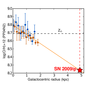
Figure 23.— Metallicity profile of NGC 7259, the host galaxy of SN 2009ip, as derived from our long slit spectroscopy. The solid line shows the best fit metallicity gradient. The dashed horizontal line marks the solar metallicity and the vertical dashed line marks the SN galactocentric radius. The colors distinguish measurements from opposite sides of the galaxy center. The error bars reflect propagation of the emission line flux uncertainties only. This analysis constrains the metallicity at the explosion site of SN 2009ip to be $8.2<\log(\rm{O/H})+12<8.6$ ($0.4\,Z_{\sun}<Z<0.9\,Z_{\sun}$).

The final fate of a massive star is controlled by the mass of its helium core (e.g. Woosley et al. 2007), which is strongly dependent on the initial stellar mass, rotation and composition. Metallicity has a key role in determining the mass-loss history of the progenitor, with low metallicity generally leading to a suppression of mass loss, therefore allowing lower-mass stars to end their lives with massive cores. SN 2009ip is positioned in the outskirts of NGC 7259 (Fig. 1). The remote location of SN 2009ip has been discussed by Fraser et al. (2013). Our data reveal no evidence for an H II region in the vicinity of SN 2009ip that would allow us to directly measure the metallicity of the immediate environment. Thus, we inferred the explosion metallicity by measuring the host galaxy metallicity gradient. The longslit was placed along the galaxy center at parallactic angle. We extracted spectra of the galaxy at positions in a sequence across our slit, producing a set of integrated light spectra from $\sim 0-2$ kpc from either side of the galaxy center.

We use the “PP04 N2” diagnostic of Pettini & Pagel (2004) to estimate gas phase metallicity using the H$\alpha$ and [N II] $\lambda 6584$ emission lines. We estimate the uncertainty in the metallicity measurements by Monte Carlo propagation of the uncertainty in the individual line fluxes. The median uncertainty is $0.09$ dex, which is similar to the systematic uncertainty in the calibration of the strong line diagnostic (Kewley & Ellison, 2008). Robust metallicity profiles can not be recovered in other diagnostics due to the faintness of the [O III] lines in our spectroscopy.

Figure 23 shows the resulting metallicity profile of NGC 7259. The metallicity at the galaxy center is $\log(\rm{O/H})+12=\sim 8.8$, $\sim 1.3~{}\rm{Z}_{\odot}$ on the PP04 N2 scale, but declines sharply with radius. The metallicity profiles on each side of the galaxy center in our longslit spectrum are consistent. We therefore assume that the metallicity profile is azimuthally symmetric. We estimate the metallicity gradient by fitting a linear profile. The best fit gradient intercept and slope are $8.8\pm 0.02$ dex and $-0.11\pm 0.02~{}\rm{dex~{}kpc^{-1}}$, respectively.

SN 2009ip is located $\sim 43.4"$ from the center of the galaxy NGC 7259 (equal to $\sim 5.0$ kpc at $d_{\rm{L}}=24\,\rm{Mpc}$). This is more than twice the distance to which our metallicity profile observations extend. Extrapolating directly from this gradient would imply an explosion site metallicity of $\log(\rm{O/H})+12=\sim 8.2$, or $\sim 0.4~{}\rm{Z}_{\odot}$. This metallicity would place SN 2009ip at the extreme low metallicity end of the distribution of observed host environments of Type II SN (Stoll et al., 2012), and nearer to the low metallicity regime of broad-lined Type Ic supernovae (Kelly & Kirshner, 2012; Sanders et al., 2012). However, the metallicity properties of galaxies at distances well beyond a scale radius have not been well studied. It is likely that a simple extrapolation is not appropriate, and the metallicity profile in the outskirts of the galaxy may flatten (Werk et al., 2011) or drop significantly (Moran et al., 2012). In either case, it is unlikely that the explosion site metallicity is significantly enriched relative to the gas we observe at $R\sim 2$ kpc, with $\log(\rm{O/H})+12\sim 8.6$ ($\sim 0.9~{}\rm{Z}_{\odot}$). If we adopt this value as the explosion site metallicity, it is fully consistent with the observed distribution of SNe II, Ib, and Ic (Kelly & Kirshner, 2012; Sanders et al., 2012; Stoll et al., 2012).

Our best constraint on the explosion site metallicity is therefore $0.4\,Z_{\sun}<Z<0.9\,Z_{\sun}$, pointing to a (mildly) sub-solar environment.

6. Energetics of the explosion

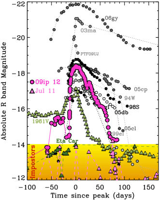
Figure 24.— Absolute R-band magnitude of SN 2009ip (pink dots) compared to the sample of Type IIn SNe with R-band photometric coverage around the peak (from the literature). For SNe 1994W, 1998S, 1999el, 2003ma, 2005cp, 2005cl, 2005db, 2005gl and 2006gy we refer the reader to Kiewe et al. (2012) and references therein. The photometry of PTF09UJ has been presented by Ofek et al. (2010). Colored area: typical absolute magnitude of LBV-like eruption episodes. Pink triangles mark the luminosity of SN 2009ip during the 2011 outburst ($t=0$ corresponds here to 2011 July 8 for convenience). The exceptional SN (impostor?) SN1961V (photographic plate magnitudes, from Pastorello et al. 2012) and $\eta$ Carinae during the 19th century Great Eruption ($M_{vis}$ as compiled by Frew 2004, see also Smith & Frew 2011) are shown with green triangles. The comparison with SN 2010mc is shown in Fig. 30.

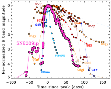
Figure 25.— Re-normalized R-band magnitude of SN 2009ip compared with the sample of SNe IIn of Fig. 24. Shades of orange (blue) are used for SNe with a slower (faster) rise time. SN 2009ip is characterized by a fast rise and fast decay.

The extensive photometric coverage (both in wavelength and in time) gives us the opportunity to accurately constrain the bolometric luminosity and total energy radiated by SN 2009ip. SN 2009ip reaches a peak luminosity of $L_{\rm{pk}}=(1.7\pm 0.1)\times 10^{43}\rm{erg\,s^{-1}}$ (Fig. 11). The total energy radiated during the 2012a outburst (from 2012 August 1 to September 23) is $(1.5\pm 0.4)\times 10^{48}\rm{erg}$ while for the 2012b explosion we measure $E_{\rm{rad2}}=(3.2\pm 0.3)\times 10^{49}$ erg. As much as $\sim 35$% of this energy was released before the peak, while $50$% of $E_{\rm{rad2}}$ was radiated during the first $\sim 15$ days. Subsequent re-brightenings (which constitute a peculiarity of SN 2009ip) only contributed to small fractions of the total energy.

The peak luminosity of SN 2009ip is not uncommon among the heterogeneous class of SNe IIn, corresponding to $M_{\rm{R}}\approx-18$ mag (Fig. 24). Its radiated energy of $(3.2\pm 0.3)\times 10^{49}$ erg falls instead into the low energy tail of the distribution mainly because of the very rapid rise and decay times of the bolometric luminosity (Fig. 25). The limited energy radiated by SN 2009ip brings into question the final fate of the progenitor star: was the total energy released sufficient to fully unbind the star (i.e., terminal explosion) or does SN 2009ip results from a lower-energy ejection of only the outer stellar envelope (i.e., non-terminal explosion)? This topic is explored in Section 8. Indeed, stars might be able to survive eruptive/explosive events that reach a visual absolute magnitude of $M_{\rm{vis}}\approx-17$ mag (e.g. SN 1961V in Fig. 25, Van Dyk & Matheson 2012, Kochanek et al. 2011), so that the peak luminosity is not a reliable indicator of a terminal vs. non-terminal explosion. With an estimated radiated energy of $3.2\times 10^{49}$ erg (Davidson & Humphreys, 1997) the ”Great Eruption” of $\eta$-Carinae (see e.g. Smith 2013 and references therein) demonstrated that it is also possible to survive the release of comparable amount of energy, even if on time scales much longer than those observed for SN 2009ip (the ”Great Eruption” lasted about 20 yrs).

SN 2010mc shows instead striking similarities to SN 2009ip both in terms of timescales and of released energy (Fig. 30). As in SN 2009ip, a precursor bump was detected $\sim 40$ days before the major outburst. Ofek et al. (2013b) calculate $E_{\rm{rad}}>6\times 10^{47}\rm{erg}$ (precursor-bump) and $E_{\rm{rad}}\sim 3\times 10^{49}\rm{erg}$ (major outburst) for SN 2010mc, compared with $E_{\rm{rad1}}=(1.5\pm 0.4)\times 10^{48}\rm{erg}$ and $E_{\rm{rad2}}=(3.2\pm 0.3)\times 10^{49}\rm{erg}$ we calculated above for SN 2009ip. The very close similarity of SN 2010mc and SN 2009ip originally noted by Smith et al. (2013) has important implications on the nature of both explosions (see Section 8).

7. Source of energy and properties of the immediate environment

In the previous sections we concentrated on the properties of the explosion (e.g. energetics, evolution of the emission/absorption features) and of the environment (i.e. the metallicity) that can be directly measured; here we focus on properties that can be inferred from the data.

The light-curve of SN 2009ip shows two major episodes of emission: the precursor bump (2012a outburst) and the major re-brightening (2012b explosion). Is this phenomenology due to two distinct explosions or is the double-peaked light-curve the result of a single explosion? The main argument against a single explosion producing the two peaks is the observed evolution of the photospheric radius in Fig. 11. In the single-explosion scenario material can only decelerate with time: at $t_{\rm{pk}}+7$ days the photospheric radius is $R_{\rm{HOT}}\sim 1.2\times 10^{15}\rm{cm}$ and the velocity is $v=4500\,\rm{km\,s^{-1}}$. Extrapolating back in time, this implies that the zero-time of the 2012b explosion is later than $t_{\rm{pk}}-24$ days. This is much later than the observed onset of the 2012a outburst that occurred at $t_{\rm{pk}}-56$ days and favors against a single-explosion scenario. Models where the first bump in the light-curve is a SN explosion while the second peak is due to the interaction of the SN ejecta with the CSM (Mauerhan et al. 2013) belong to this category. In the following we proceed instead with a two-explosion hypothesis and argue that we witnessed two separate but causally connected explosions from the progenitor of SN 2009ip.

7.1. Limit on the Nickel mass synthesized by the 2012b explosion

Narrow emission lines in the optical spectra of SN 2009ip require that interaction with previously ejected material (either in the form of a stable wind or from erratic mass-loss episodes) is occurring at some level. The multiple outbursts of SN 2009ip detected in the 2009, 2011 and August 2012 (from 3 years to $\sim 1$ month before the major 2012 explosion) are likely to have ejected conspicuous material in the immediate progenitor surroundings so that interaction of the 2012b explosion shock with this material qualifies as an efficient way to convert kinetic energy into radiation.

The radioactive decay of ${}^{56}\rm{Ni}$ represents another obvious source of energy. We employ the nebular phase formalism developed by Valenti et al. (2008) (expanding on the original work by Sutherland & Wheeler 1984 and Cappellaro et al. 1997) to constrain the amount of Nickel synthesized by the 2012b explosion using late time observations. If the observed light-curve were to be entirely powered by the energy deposition of the ${}^{56}\rm{Ni}$ radioactive decay chain, our latest photometry would imply $M_{\rm{Ni}}\sim 0.03\,\rm{M_{\sun}}$ for a standard explosion kinetic energy of $E_{k}=10^{51}\,\rm{erg}$. For a low energy explosion with $E_{k}=10^{50}\,\rm{erg}$, $M_{\rm{Ni}}\sim 0.08\,\rm{M_{\sun}}$. Allowing for other possible sources of energy contributing to the observed luminosity (like interaction), we conclude $M_{\rm{Ni}}<0.08\,\rm{M_{\sun}}$. Using this value (and the photospheric formalism by Valenti et al. 2008, based on Arnett 1982) we largely underpredict the luminosity of SN 2009ip at peak for any value of mass and kinetic energy of the ejecta: the energy release of SN 2009ip is therefore not powered by ${}^{56}\rm{Ni}$ radioactive decay. Fraser et al. (2013) independently derived $M_{\rm{Ni}}<0.02\,\rm{M_{\sun}}$, consistent with our findings. In the following we explore a model where the major UV-bright peak is powered by shock break-out from a dense shell ejected by the precursor bump, while continued interaction with previously ejected material is responsible for the peculiar, bumpy light-curve that follows.

7.2. Shock break-out plus continued interaction scenario for the 2012b explosion

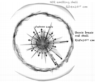
Figure 26.— Sketch of SN 2009ip. Its environment as well as its ejecta are likely to have an extremely complex, potentially asymmetric structure. Here we show the basic components of the 2012b explosion and its environment. In the ejecta we recognize the presence of three velocity components at $v\sim 2500\,\rm{km\,s^{-1}}$, $v\sim 5000\,\rm{km\,s^{-1}}$ together with very fast material at $v>10000\,\rm{km\,s^{-1}}$ (Fig. 22). Shock break-out from a dense shell of material left over by the 2012a outburst is responsible for the major peak in the light-curve (Section 7.2). Material sitting at larger distance, connected with previous episodes of eruption, is responsible for partially re-processing the radiation into the NIR band, producing the NIR excess of Fig. 13 (Sec. 7.8). Our analysis requires this material to have a low filling factor and/or asymmetric distribution.

The rapid rise and decay times of the major 2012b explosion (Fig. 25) suggest that the shock wave is interacting with a compact shell(s) of material. The relatively fast fading of CSM-like features and subsequent emergence of Type IIP features shown in Fig. 21 supports a similar conclusion. The bumps in the light-curve further suggest an inhomogeneous medium. We consider a model where the ejecta from the 2012b explosion initially interact with an optically thick shell of material, generating the UV-bright, major peak in the light-curve (Fig. 26). In our model, the light-curve is powered at later times by interaction with optically thin material.

In the shock break-out scenario the escape of radiation is delayed with respect to the onset of the explosion until the shock is able to break-out from the shell at an optical depth $\tau_{\rm{w}}\approx c/v_{\rm{sh}}$. This happens when the diffusion time $t_{\rm{d}}$ becomes comparable to the expansion time. Radiation is also released on the diffusion time scale, which implies that the observed bolometric light-curve rise time is $t_{\rm{rise}}\approx t_{\rm{d}}$. Following Chevalier & Irwin (2011), the radiated energy at break-out $E_{\rm{rad}}$, the diffusion time $t_{\rm{d}}$ and the radius of the contact discontinuity at $t=t_{\rm{d}}$ ($\equiv R_{\rm{bo}}$) depend on the explosion energy $E$, the ejecta mass $M_{\rm{ej}}$, the environment density $\rho_{\rm{w}}$ (parametrized by the progenitor mass-loss rate) and opacity $k$. From our data we measure: $t_{\rm{rise}}\approx 10$ days; $R_{\rm{bo}}\approx 5\times 10^{14}$ cm; $E_{\rm{rad}}\approx 1.3\times 10^{49}$ erg. We solve the system of equations for our observables in Appendix A and obtain the following estimates for the properties of the explosion and its local environment. Given the likely complexity of the SN 2009ip environment, those should be treated as order of magnitudes estimates.

The onset of the 2012b explosion is around 20 days before peak (2012 September 13). Using Eq. A2 and Eq. A3, the progenitor mass-loss rate is $\dot{M}\approx 0.07(v_{\rm{w}}/200\,\rm{km\,s^{-1}})\rm{M_{\sun}yr^{-1}}$. We choose to renormalize the mass-loss rate to $200\,\rm{km\,s^{-1}}$, which is the FWHM of the narrow emission component in the H$\alpha$ line (e.g. Fig. 16). The observed bolometric luminosity goes below the level of the luminosity expected from continued interaction of Eq. A6 around $32$ days after the onset of the explosion or $t_{\rm{pk}}+12$ days. By this time she shock must have reached the edge of the dense wind shell: $t_{\rm{w}}\lesssim 32$ days. This constrains the wind shell radius to be $R_{\rm{w}}\approx 1.2\times 10^{15}\rm{cm}$ (Eq. A7), therefore confirming the idea of a compact and dense shell of material, while the total mass in the wind shell is $M_{\rm{w}}\approx 0.1\rm{M_{\sun}}$ (Eq. A5). The system of equations is degenerate for $M_{\rm{ej}}/E^{2}$. Adopting our estimates of the observables above and Eq. A1 we find $M_{\rm{ej}}\approx 50.5(E/10^{51}\rm{erg})^{2}\rm{M_{\sun}}$. The efficiency of conversion of kinetic energy into radiation depends on the ratio of the total ejecta to wind shell mass (e.g. van Marle et al. 2010; Ginzburg & Balberg 2012; Chatzopoulos et al. 2012). This suggests $M_{\rm{ej}}\approx M_{\rm{w}}$ as order of magnitude estimate, from which $E\sim 10^{50}\,\rm{erg}$.

After $t_{\rm{w}}$ the bolometric luminosity starts to decay faster, especially at UV wavelengths (Fig. 2). By this time the shock has overtaken the dense thick shell and starts to interact with less dense, optically thin layers of material producing continued power for SN 2009ip. In this regime the observed luminosity tracks the energy deposition rate: $L=4\pi R^{2}\rho_{\rm{w}}(v_{\rm{fs}}-v_{\rm{w}})^{3}$, where $R$ is the radius of the cold dense shell that forms as a result of the loss of radiative energy from the shocked region; $v_{\rm{fs}}$ is the forward shock velocity; $v_{\rm{w}}$ and $\rho_{\rm{w}}$ are the velocity and density of the material encountered by the shock wave (Chevalier & Irwin 2011 and references therein). The presence of clearly detected bumps in the bolometric light-curve (with associated rise in the effective temperature of the radiation, Fig. 11) suggests that the medium has a complex structure and it is likely inhomogeneous. consequently $\rho_{\rm{w}}$ might significantly depart from the $\propto R^{-2}$ profile expected in the case of steady wind. The increasing FWHM with time measured for the narrow component of the H$\alpha$ line in Fig. 16 points to larger $v_{\rm{w}}$ at larger distances from the explosion, therefore deviating from the picture of a steady wind with constant $v_{\rm{w}}$ (see Section 7.3). Given the complexity of the explosion environment, we adopt a simplified shock interaction model (see e.g. Smith et al. 2010a) and parametrize the observed luminosity as: $L=(\eta/2)wv^{3}$, where $\eta$ is the efficiency of conversion of kinetic energy into radiation; $w(R)\equiv\dot{M}/v_{\rm{w}}$ (hence $\rho_{\rm{w}}=w(R)/4\pi R^{2}$); while $v$ is a measure of the expansion velocity of the shock into the environment. We estimate $v$ from the evolution of the black-body radius with time ($v\approx\dot{R}_{\rm{HOT}}$ of Fig. 11), assuming that for $t_{\rm{pk}}+17$ days the true shock radius continues to increase with $v\approx 4500\,\rm{km\,s^{-1}}$ (while the measured $R_{\rm{HOT}}$ stalls and then decreases as the interaction shell progressively transitions to the optically thin regime, see Section 3). Using the bolometric luminosity of Fig. 11, we can therefore constrain the properties (density and mass) of the environment as sampled by the 2012b explosion.

We find that the total mass swept up by the shock from $t_{\rm{w}}=32$ days until the end of our monitoring (112 days since explosion) is $M_{\rm{w}}^{\rm{thin}}\approx(0.05/\eta)\rm{M_{\rm{\sun}}}$. The total mass in the environment swept up by the 2012b explosion shock is therefore $M_{\rm{tot}}=M_{\rm{w}}+M_{\rm{w}}^{\rm{thin}}\approx(0.2-0.3)\rm{M_{\rm{\sun}}}$ for $\eta=50-30\%$. As a comparison, Ofek et al. (2013a) derive a mass of $\sim 0.1\rm{M_{\rm{\sun}}}$. Our analysis points to a steep density profile with $\rho_{\rm{w}}\propto R^{-5.3}$ for $R>1.4\times 10^{15}\rm{cm}$. The mass-loss rate is $\dot{M}(R)=w(R)v_{\rm{w}}(R)$. We estimate $v_{\rm{w}}$ from the evolution of the FWHM of the narrow H$\alpha$ component in Fig. 16. Combining this information with the expression above we find $\dot{M}(R)\propto R^{-2}$ for $(1.4<R<4.4)\times 10^{15}\rm{cm}$, with $\dot{M}(R)\approx(0.08/\eta)\rm{M_{\sun}/yr}$ at $R=1.4\times 10^{15}\rm{cm}$, declining to $(0.008/\eta)\rm{M_{\sun}/yr}$ at $R=4.4\times 10^{15}\rm{cm}$.

7.3. Origin of the interacting material in the close environment

During the 2012b explosion, the shock interacts with an environment which has been previously shaped by the 2012a explosion and previous eruptions. In this section we infer the properties of the pre-2012a explosion environment, using the 2012a outburst as a probe. We look to: (i) understand the origin of the compact dense shell with which the 2012b shock interacted, whether it is newly ejected material by the 2012a outburst or material originating from previous eruptions; (ii) constrain the nature of the slowly moving material ($v\approx$ a few $100\,\rm{km\,s^{-1}}$) responsible for narrow line emission in our spectra.

We put an upper limit on the total amount of mass in the surroundings of SN 2009ip before the 2012a explosion assuming that the observed luminosity of the 2012a outburst is entirely powered by optically thin shock interaction with some previously ejected material of mass $M_{\rm{w}}^{\rm{12a}}$. As before: $L=(\eta/2)wv^{3}$. $M_{\rm{w}}^{\rm{12a}}=\int w(R)dR$. The evolution of the black-body radius of Fig. 11 suggests $v\approx 2500\,\rm{km\,s^{-1}}$ before 2012 August 21. We apply the same line of reasoning as above and assume that the shock continues to expand with this velocity, while the photosphere transitions to the thin regime and stalls at $\approx 0.4\times 10^{15}\,\rm{cm}$. In this picture, the 2012a shock sampled the environment on distances $R<1.2\times 10^{15}\rm{cm}$, sweeping up a total mass of $M_{\rm{w}}^{\rm{12a}}\leq(0.02/\eta)\rm{M_{\sun}}$. In Section 7.2 we estimated that the total mass of the dense wind shell from which the 2012b shock breaks out is $M_{\rm{w}}\approx 0.1\,\rm{M_{\sun}}$ with radius $R_{\rm{w}}\approx 1.2\times 10^{15}\rm{cm}$. The wind shell mass is $M_{\rm{w}}=M_{\rm{w}}^{\rm{12a}}(R<R_{\rm{w}})+M_{\rm{ej}}^{\rm{12a}}(R<R_{\rm{w}})$, where $M_{\rm{ej}}^{12a}(R<R_{\rm{w}})$ is the portion of the ejecta mass of the 2012a explosion within $R_{\rm{w}}$ at $t=t_{\rm{w}}$. This implies $M_{\rm{ej}}^{12a}(R<R_{\rm{w}})>0.06\,\rm{M_{\sun}}(>0.09\,\rm{M_{\sun}})$ for our fiducial efficiency $\eta=30\%$ ($\eta=50\%$), comparable with the mass of the dense wind shell. We conclude that the UV-bright 2012b explosion results from shock break-out from a dense shell which mostly (if not entirely) originates from the ejecta mass of the 2012a explosion, therefore establishing a direct connection between the properties of the 2012a-2012b episodes.

The previous result also implies a solid lower limit on the total ejecta mass of the 2012a outburst: $M_{\rm{ej}}^{12a}>0.06\,\rm{M_{\sun}}(>0.09\,\rm{M_{\sun}})$ for $\eta=30\%$ ($\eta=50\%$). In Section 7.2 we estimated that the total mass collected by the 2012b shock by the end of our monitoring is $M_{\rm{tot}}\approx 0.2-0.3\,\rm{M_{\sun}}$, which constrains $0.06<M_{\rm{ej}}^{12a}<0.3\,\rm{M_{\sun}}$ for $\eta\geq 30$%. In the following we use $M_{\rm{ej}}^{12a}\approx 0.1\rm{M_{\sun}}$ as an order of magnitude estimate for the mass ejected by the 2012a outburst.

Our spectra show evidence for narrow line emission (Section 4) typically observed in SNe IIn (and LBVs), which is usually interpreted as signature of the ejecta interaction with material deposited by the progenitor wind before explosion. For SN 2009ip we observe during the 2012b event a velocity gradient in the narrow emission from H$\alpha$ (Fig. 16, panel c), with increasing velocity with time. This increase is consistent with being linear with time. This might suggest a Hubble-like expansion for the CSM following the simple velocity profile $v\propto R$: as time goes by, the shock samples material at larger distances from the explosion (hence with larger velocity $v$). Our analysis indicates that episodes of mass ejection with approximate age 11-19 months before the 2012b explosion (roughly between February and October 2011) might reasonably account for the observed velocity gradient. We suggest that CSM material in the surroundings of SN 2009ip moving at velocities of hundreds $\rm{km\,s^{-1}}$ originates from this sudden episode(s) of mass ejection. Remarkably, SN 2009ip has been reported to be in eruptive phase between May and October 2011 (Pastorello et al., 2012), consistent with this picture.

The Hubble-like flow is not consistent with a steady wind and points instead to some mechanism leading to explosive mass ejections. Interestingly, it is during the September 2011 outburst that SN 2009ip showed evidence for material with unprecedented velocity, reaching $v=12500\,\rm{km\,s^{-1}}$ (Pastorello et al., 2012). Since no line-driven or continuum-driven wind mechanism is known to be able to accelerate stellar surface material to these velocities (Mauerhan et al. 2013), stellar-core related mechanisms have to be invoked. The explosive mass ejection suggested by our analysis might therefore be linked to instabilities developing deep inside the stellar core.

7.4. The role of asymmetries in SN 2009ip

The analysis of Section 4.5 indicates the presence of ejecta traveling at three distinct velocities: $v\sim-12000\,\rm{km\,s^{-1}}$, $v\sim-5500\,\rm{km\,s^{-1}}$ and $v\sim-2500\,\rm{km\,s^{-1}}$. These values correspond to the velocity of material seen in absorption (i.e. placed outside the photosphere). The radius of the hot blackbody $R_{\rm{HOT}}$ of Fig. 11 tracks the position of the photosphere with time. Assuming free expansion of the ejecta and the explosion onset time ($t_{\rm{pk}}-20$ days) derived in the previous sections, we can predict at which time $t_{v}$ ejecta moving at a certain velocity $v$ will overtake the photosphere at $R_{\rm{HOT}}$. Only for $t\gtrsim t_{v}$ can the ejecta give rise to absorption features in the spectra. Spherical symmetry is an implicit assumption in the calculation of $R_{\rm{HOT}}$, so that comparing the predicted $t_{v}$ to the observed time of appearance of the absorption edges makes it possible to test the assumption of spherical symmetry of the explosion.

For $v\sim-2500\,\rm{km\,s^{-1}}$ we find $t_{\rm{v}}=t_{\rm{pk}}+55$ days (2012 November 27) in excellent agreement with our observations, which constrain the $v\sim-2500\,\rm{km\,s^{-1}}$ absorption edge to appear between 2012 November 23 and December 5 (Fig: 22). No departure from spherical symmetry needs to be invoked for slow-moving ejecta, which likely includes most of the ejecta mass. Spherical symmetry is instead clearly broken by the high-velocity material traveling at $v\sim-12000\,\rm{km\,s^{-1}}$. For the 2012b explosion we detect high velocity material in absorption starting from $\sim 1$ week after peak. Around peak the spectrum of SN 2009ip is optically thick and shows no evidence for material with $v\sim-12000\,\rm{km\,s^{-1}}$ (Fig. 19 and Fig. 20). However, in no way could a perfectly spherical photosphere traveling at $4000-5000\,\rm{km\,s^{-1}}$ mask the fast-moving ejecta at any time during the evolution, and in particular until the first week after peak, as we observed. This indicates a departure of the high-velocity ejecta from spherical geometry and might suggest the presence of a preferred direction in the explosion.

Asymmetry can also have a role in the spatial distribution of the interacting material, as supported by the observed co-existence of broad and (unresolved) intermediate components in the spectrum (Fig. 14). In this respect, Chugai & Danziger (1994) proposed the possibility of an enhanced mass loss on the equatorial plane of SNe IIn to explain the intermediate velocity component in SN 1988Z, other explanations being a clumpy circumstellar medium or, again, an asymmetric flow. In this context it is worth noting that asymmetry is also a likely explanation for the discrepant mass-loss estimates found by Ofek et al. (2013a), as noted by the authors. A disk-like geometry for SN 2009ip was proposed by Levesque et al. (2012) based on the H Balmer decrement. Finally, the binary-star merger scenario proposed by Soker & Kashi (2013) to interpret SN 2009ip naturally leads to ejecta with a bipolar structure.

7.5. Hard X-rays and X-rays from shock break-out and continued interaction

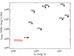
Figure 27.— Radio luminosity at peak vs. X-ray luminosity at the radio peak for a sample of Type IIn SNe (black dots). SN 2009ip is shown in red. Data have been collected from the literature. (See Pooley et al. 2002; Smith et al. 2007; Stritzinger et al. 2012; Chandra et al. 2012a; Pooley et al. 2007; Chandra & Soderberg 2007; Chandra et al. 2009; Zampieri et al. 2005; Houck et al. 1998; Chevalier 1987; van Dyk et al. 1993; Fabian & Terlevich 1996; and references therein).

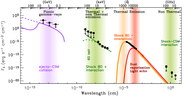
Figure 28.— Broad-band SED of SN 2009ip around the optical peak. Shaded bands highlight different components of emission that dominate at different wavelengths. Neutral pion decay leads to $\gamma$-rays which are ultimately powered by the collision between the ejecta and extremely dense CSM shells of material. We show here the limits obtained by Fermi-LAT in the week around maximum light (from $t=t_{\rm{pk}}-2$ days until $t=t_{\rm{pk}}+4$ days). Dashed purple line: expected GeV emission based on the shock explosion parameters derived in Section 7.2 and the model by Murase et al. (2011) assuming no attenuation. The thick-line model includes partial attenuation as relevant for a clumpy and/or asymmetric medium (Sec. 7.4) with filling factor $<1$ that reduces the effects of the Bethe-Heitler process. Soft and hard X-ray emission originates from the interaction of the shock with the CSM: both thermal and non-thermal emission might arise, mainly depending on the environment density. We show here a power-law (non-thermal emission, thick line with $F_{\lambda}\propto\lambda^{-2.4}$) and a thermal bremsstrahlung model with $kT=60$ keV (dashed line) that fit the Swift-XRT 0.3-10 keV data obtained between $t_{\rm{pk}}-2$ days and $t_{\rm{pk}}+4$ days. Swift-BAT 15-150 keV data acquired at $t_{\rm{pk}}\pm 1$ days are also shown. The dotted line marks the energy of 60 keV: this is the typical frequency of high-energy photons emitted by the collisionless shock that forms at shock break-out (Katz et al. 2011). Optical and UV emission is powered by the shock break-out plus continued shock interaction with the environment. The orange thick line is the best-fitting ”hot” black-body component with $T\approx 17000$ K obtained at maximum light. NIR and IR emission could originate from dust formation, dust vaporization but it might also be a light echo. Due to the high temperature we infer ($T\approx 3000$ K, red solid line) we favor dust vaporization here. Shock-CSM interaction is also the source of millimeter and radio photons through synchrotron emission. At these times this emission was quenched by free-free absorption by the dense shell of material.

SN 2009ip is a weak X-ray and radio emitter (Fig. 27). In the following two sections we connect the lack of high X-ray/radio luminosity to the shock break-out plus interaction scenario we developed to explain the optical properties of SN 2009ip.

The shock break-out plus continued interaction scenario gives rise to a two-component spectrum, with a hard (X-rays) and a soft (UV/optical, at the break-out velocity of interest here) component (e.g. Svirski et al. 2012; Chevalier & Irwin 2012). The hard component is generated by bremsstrahlung emission from hot electrons behind the shock. Theory predicts that $L_{\rm{hard,bo}}\sim 10^{-4}L_{\rm{bo}}$ (where $L_{\rm{bo}}$ is the break-out luminosity, resulting from the soft and hard component) as long as: (i) Inverse Compton (IC) cooling dominates over bremsstrahlung; (ii) high-energy photons undergo Compton degradation in the unshocked wind during their diffusion to the observer. We show in the following that both processes are relevant for SN 2009ip and provide a natural explanation for its very low X-ray to optical luminosity ratio ($L_{\rm{x}}/L_{\rm{optical}}\lesssim 10^{-4}$).

From our modeling of Section 7.2, we inferred a density parameter $D_{*}\approx 0.4$ (where $D_{*}$ is a measure of the density of the dense wind shell $\rho_{\rm{w}}$, as explained in Appendix A). With a shock velocity $v\approx 4500\,\rm{km\,s^{-1}}$, the density measurement above implies that around break-out time the main source of cooling of the hot electrons is IC (see Chevalier & Irwin 2012). For our parameters, the IC to Bremsstrahlung (ff) emissivity ratio at break-out is (Svirski et al. 2012, their Eq. 17) $\epsilon^{IC}/\epsilon^{ff}\approx 0.01(v/10^{9}\rm{cm\,s^{-1}})^{2}$ or $\epsilon^{IC}/\epsilon^{ff}\approx 0.05$ for the observed $v\approx 4500\,\rm{km\,s^{-1}}$. IC is the dominant cooling source, suppressing the emission of hard photons in SN 2009ip. The calculations by Ofek et al. (2013a) instead assume negligible IC cooling.

Comptonization of the hard photons as they propagate through the unshocked wind region to the observer furthermore leads to a suppression of high-energy radiation. This process can effectively suppress photons with $\approx$keV energy if $\tau_{\rm{es}}\gtrsim 15-20$, the photon energy being limited by $\epsilon_{\rm{max}}=511/\tau_{\rm{es}}^{2}$ keV. Our modeling of Section 7.2 implies $\tau_{es}\approx 15$ for SN 2009ip around shock break-out. This demonstrates that both the domination of IC over bremsstrahlung (i) and Compton losses (ii) are relevant to explain the weak X-ray emission in SN 2009ip. Identifying $L_{\rm{x}}$ with $L_{\rm{hard}}$ and $L_{\rm{bol}}$ with $L_{\rm{bo}}$, the shock break-out scenario therefore naturally accounts for the observed $L_{\rm{x}}/L_{\rm{optical}}\lesssim 10^{-4}$ ratio even in the absence of photo-absorption.

Chevalier & Irwin (2012) calculate that full ionization (which gives minimal photo-absorption) is achieved for high-velocity shocks with $v\gtrsim 10^{4}\rm{km\,s^{-1}}$. For SN 2009ip $v\approx 4500\,\rm{km\,s^{-1}}$ likely leads to incomplete ionization (i.e. potentially important photo-absorption), that will further reduce the escaping X-ray flux. Using the explosion observables and Eq. A9 we constrain the total column density between the shock break-out radius and the observer to be $N\approx 2\times 10^{25}\rm{cm^{-2}}$ which gives a bound-free optical depth $\tau_{\rm{bf}}\approx 2\times 10^{3}$ at 1 keV (Eq. A10). Since $\tau_{\rm{bf}}\propto R^{-1}$ and $R\propto t$, soft ($E\approx 2$ keV) X-ray emission would not be expected from SN 2009ip until $R\approx 2\times 10^{16}\rm{cm}$ which happens for $\Delta t\gtrsim 440$ days since the explosion, or $\gtrsim 44$ break-out time scales $t_{\rm{d}}$ (where $t_{\rm{d}}\approx t_{\rm{rise}}$ in our scenario). This calculation assumes an extended and spherically symmetric wind profile. The Chandra detection of SN 2009ip at much earlier epochs ($\Delta t\approx 4\,t_{\rm{d}}$) indicates that at least one of these assumptions is invalid, therefore pointing to a truncated and/or highly asymmetric wind profile. This is consistent with the picture of a dense but compact wind shell of radius $R_{\rm{w}}\approx 1.2\times 10^{15}\rm{cm}$ followed by a steep density gradient $\rho_{\rm{w}}\propto R^{-5.3}$ we developed in Section 7.2. Asymmetry also plays a role, as independently suggested by observations in the optical (Section 7.4).

Finally, Katz et al. (2011) predict that hard-X-ray emission with typical energy of $60$ keV is also produced by the collision-less shock. The details of the spectrum are however unclear. Bound-free absorption is less important at these energies giving the chance to detect hard X-rays at earlier times. Our Swift-BAT campaign in the 15-150 keV range revealed a tentative detection. With these observations we put a solid upper limit on the hard X-ray to optical luminosity around maximum light which is $L_{\rm{X,hard}}/L_{\rm{bol}}<5\times 10^{-3}$ at $5\sigma$. The broad band SED around maximum light is shown in Fig. 28.

7.6. Radio emission from shock break-out and continued interaction

The shock-CSM interaction is a well known source of radio emission (e.g. Chevalier 1982; Chevalier 1984). The limited shock velocity we infer for SN 2009ip likely leads to a partially ionized medium as discussed above, so that free-free absorption plays a key role in suppressing the emitted radio flux. We quantify this statement below. The high density of the wind shell derived from our modeling of Section 7.2 implies a free-free optical depth at radius $R$, $\tau_{\rm{ff}}\approx 3.8\times 10^{54}(\nu/\rm{GHz})^{-2.1}(R/\rm{cm})^{-3}$ (Eq. A11). With $\tau_{\rm{ff}}\approx 10^{5}-10^{8}$ at $R\approx R_{\rm{bo}}$, no detectable radio emission is expected around break-out, consistent with our lack of radio detection around these times. If the dense wind profile extends out to large distances, the calculation above shows that no radio emission is expected until very late times, when the shock reaches $R\approx 7\times 10^{16}\rm{cm}$. Our radio detection at much earlier epochs ($\Delta t\approx 60-80$ days since explosion) demonstrates instead that the dense wind shell is not extended but truncated and adds further, independent evidence for a complex medium where inhomogeneity, asymmetry and/or low wind filling factor might also be relevant. This is consistent with the idea we suggested in Section 7.3 that the dense shell was the outcome of a short eruption, since eruptions are more likely to eject shells with sharp density edges as opposed to a steady mass loss.

7.7. GeV and neutrino emission at shock break-out

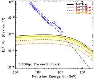
Figure 29.— Predicted muon and anti-muon neutrino fluence from SN 2009ip using the observables and explosion parameters of Sec. 7.2 according to the model by Murase et al. (2011). The shaded band corresponds to different values for the total energy in cosmic rays $E_{\rm{CR}}$ here parametrized as a function of the radiated energy at $t_{\rm rise}$. Note that, given $E_{k}\gg E_{\rm rad}$, larger values of $E_{\rm CR}$ are also possible. Dashed blue line: atmospheric neutrino background integrated over $\Delta t\approx t_{\rm{rise}}$ (zenith-angle averaged within 1$\arcdeg$), which is shown for comparison. For this event, the atmospheric neutrino background is more severe since SN 2009ip occurred in the southern hemisphere. For better localized explosions, this plot shows how limits on the neutrino emission can be used to constrain $E_{\rm{CR}}$.

In the previous sections we suggested the presence of a dense ($n\approx 4\times 10^{10}\rm{cm^{-3}}$ at the break-out radius) and compact shell in the close environment of SN 2009ip that we associate with material ejected during the 2012a outburst. Shock break-out from this shell powers the major re-brightening of SN 2009ip at optical wavelengths (2012b explosion) and naturally explains the weak radio and X-ray emission we observe. The collision of the ejecta with massive shells is also expected to accelerate cosmic rays (CRs) and generate GeV gamma-rays (Murase et al. 2011; Katz et al. 2011) with fluence that depends both on the explosion and on the environment parameters. The GeV emission is expected to be almost simultaneous with the UV-optical-NIR emission. The proximity of SN 2009ip ($\approx 24$ Mpc) justifies the first search for GeV emission from shock break-out. Fermi-LAT observations covering the period 2012 September 3 – October 31 ($t_{\rm{pk}}-30$ days until $t_{\rm{pk}}+28$ days) yielded no detection (Sec. 2.10). Following Murase et al. (2011), we predict the GeV emission from SN 2009ip (2012b outburst) using the explosion and environment parameters inferred in Sec. 7.2 (shell density $\rho_{\rm{w}}$ or mass $M_{\rm{w}}$) together with the observables of the system ($t_{\rm{rise}}$, $R_{\rm{bo}}$). We take into account the attenuation due to $\gamma\gamma\rightarrow e^{+}e^{-}$ pair production, assuming a black-body spectrum with $T=20000$ K. The attenuation by extragalactic background light is also included. Since $n$ is not too large, the Bethe-Heitler pair production will be irrelevant in our case, as it happens for a clumpy or asymmetric CSM (Sec. 7.4) with filling factor $<1$. The injected CR energy $E_{\rm CR}$ is assumed to be equal to that of the radiation energy at $t_{\rm rise}$. We compare the expected GeV fluence with observations in Fig. 28: the Fermi-LAT non-detection is consistent with our picture of ejecta crashing into a compact and dense but low-mass ($\lesssim 0.1-0.2\,\rm{M_{\sun}}$) shell of material at small radius that we developed in the previous sections. For the detection of $\gamma-$rays, brighter SNe (closer SNe or SNe accompanying larger dissipation) are needed.

Using the set of parameters above we predict the muon and anti-muon neutrino fluence from SN 2009ip in Fig. 29, using the model by Murase et al. (2011). CRs produce mesons through inelastic proton-proton scattering, leading to neutrinos as well as $\gamma-$rays. As for the $\gamma-$rays, given that the explosion/ environment parameters are constrained by observations at UV/optical/NIR wavelengths, the neutrino fluence directly depends on the total energy in CRs, $E_{\rm{CR}}$ (or, equivalently on the CR acceleration efficiency $\epsilon_{\rm{CR}}$, $E_{\rm{CR}}\equiv\epsilon_{\rm{CR}}E$, being $E$ the explosion energy). Note that the injected CR energy $E_{\rm CR}$ is assumed to be the radiation energy at $t_{\rm rise}$, but larger values of $E_{\rm CR}$ are also possible. The maximum proton energy is also set to $1.5$ PeV, corresponding to $\varepsilon_{B}=0.01$. Our calculations show that SN 2009ip was a bright source of neutrinos if $E_{\rm{CR}}$ is comparable to the radiated energy. We note however that its location in the souther sky was not optimal for searches for neutrino emission by IceCube because of the severe atmospheric muon background. With this study we demonstrate how it is possible to constrain the CR acceleration efficiency if: (i) the explosion/ environment parameters are constrained by observations at UV/optical/NIR wavelengths; (ii) deep limits on muon neutrinos are available, as will be the case also for southern sky sources once KM3Net will be online in the near future.

7.8. Origin of the NIR excess

The time-resolved broad-band SED analysis of Section 3 identifies the presence of a NIR excess of emission (Fig. 13) and allows us to constrain its temporal evolution (Fig. 11). Contemporaneous NIR spectroscopy from Section 2.6 clearly shows that the NIR excess cannot be ascribed to line emission (Fig. 7), therefore pointing to a physical process producing NIR continuum emission. Adopting a black-body spectral model (with the implicit assumption of spherical symmetry) we find that: (i) the equivalent black-body radius is $R_{\rm{COLD}}\sim 4\times 10^{15}\,\rm{cm}$ with very limited evolution with time over 30 days of monitoring. This is in contrast with the hot component radius $R_{\rm{HOT}}$ which increases linearly with time inside the cooler component. (ii) The cold black-body temperature is also stable, with $T_{\rm{COLD}}\sim 3000\,\rm{K}$ (while the hot black body cools from $19000$ K to $<10000$ K). Considering that our fits can overestimate the true dust temperature of hundreds of degrees (up to 20% according to Nozawa et al. 2008) the real dust temperature might be close to $\sim 2500$ K. (iii) The resulting NIR excess luminosity is $L_{\rm{COLD}}\sim 4\times 10^{41}\rm{erg\,s^{-1}}$ which represents $(2-4)$% of $L_{\rm{HOT}}$. We use these properties to constrain the origin of the NIR excess below.

A clear spectroscopic signature of dust formation is the development of highly asymmetric and blue-shifted line profiles (see e.g. Smith et al. 2008, their Fig. 4) which is not observed. The temperature of $\sim 2500-3000$ K is also prohibitively high for dust to form. At this very early epochs the shock radius is also $<R_{\rm{COLD}}$. Note that $R_{\rm{COLD}}$, derived assuming a black-body spectrum, represents a lower limit to the real size $R_{\rm{NIR}}$ of the NIR emitting region (Fig. 26): $R_{\rm{NIR}}\propto R_{\rm{COLD}}/f^{0.5}$, where $f<1$ is the covering factor of the NIR emitting material. $f<1$ is indeed required for the hot black-body radiation to be able to escape. This clearly implies that the NIR emission cannot originate from dust created behind the reverse shock. The dust creation scenario is therefore highly unlikely, leading to the conclusion that the NIR excess originates from pre-existing material ejected by the progenitor before the 2012b explosion. Since the geometry of the NIR emitting material can be non spherical (as we find in Section 7.4) and/or have low filling factor (i.e. the material can be clumpy), we do not expect this material to necessarily produce absorption along our line of sight.

Material ejected during the 2012a outburst would be required to travel at an average velocity $v>8000\,\rm{km\,s^{-1}}$ (to reach $4\times 10^{15}\rm{cm}$ at the time of the 2012b explosion) and then to decelerate to $v<1000\,\rm{km\,s^{-1}}$ (to match the observed evolution of $R_{\rm{COLD}}$). We consider this scenario unlikely and suggest that the origin of the pre-existing material is rather linked to the eruption episodes of the progenitor of SN 2009ip in the years before. The same conclusion was independently reached by Smith et al. (2013). We note that the size of the cool emitting region of SN 2009ip is remarkably similar to the pre-outburst dust radii of other optical transients linked to eruption episodes of their progenitor stars like NGC 300 OT2008-1 ($R\sim 5\times 10^{15}\,\rm{cm}$) and SN 2008S ($R\sim 2\times 10^{15}\,\rm{cm}$, see e.g. Berger et al. 2009, their Fig. 28).

NIR emission in Type II SNe has also been connected to the extended atmosphere of the expanding star (e.g. Dwek et al. 1983). However, for SN 2009ip, the large radius we infer from our modeling ($R_{\rm{COLD}}\sim 4\times 10^{15}\,\rm{cm}$) and the lack of a clear evolution of the temperature with time argue against this interpretation.

A light echo from dust (i.e. pre-existing dust heated up by the UV and optical radiation from the explosion) would require the dust grains to survive the harsh environment. At the high temperature of $T\sim 2500-3000\,\rm{K}$ this is however unlikely, while dust vaporization is more likely to happen (see e.g. Draine & Salpeter 1979). We speculate on the dust vaporization scenario below.

In this picture a cavity is excavated by the explosion radiation out to a radius $R_{\rm{c}}$: this radius identifies the position of the vaporized dust, while it does not track the outer dust shell radius (which is instead likely to expand with time, see e.g. Pearce et al. 1992). Being the dust shell created in the years before the 2012 explosion, we expect the smaller grains to be located at the outer edge of the dust shell as a result of forces acting on them (e.g. radiative pressure). At smaller distances we are likely dominated by the larger dust grains. Following Dwek et al. (1983), their Eq. 8 (see also Draine & Salpeter 1979) the radius of the dust-free cavity for a UV-optical source with luminosity $L$ is: $R_{\rm{c}}=23(\langle Q\rangle(L/\rm{L_{\sun}})/(\lambda_{0}/\rm{\mu m})T^{5})^{0.5}$, where $R_{\rm{c}}$ is in units of pc; $T$ is the temperature at the inner boundary of the dust shell which we identify with the evaporation temperature $T_{\rm{ev}}$; $\langle Q\rangle$ is the grain emissivity: $Q=(\lambda_{0}/\lambda)^{n}$ for $\lambda\geq\lambda_{0}$ while $Q=1$ for $\lambda<\lambda_{0}$. Here we adopt $n=1$. The dust grain radius is $a$, with $\lambda_{0}\sim 2a$ which implies $R_{\rm{c}}\propto a^{-0.5}$. For $R_{\rm{c}}=R_{\rm{COLD}}\sim 4\times 10^{15}\rm{cm}$, $T_{\rm{ev}}\sim 3000$ K and $L=L_{\rm{pk}}\sim 1.7\times 10^{43}\rm{erg\,s^{-1}}$, we constrain the radius of the vaporizing dust grains to be $a\lesssim(2-5)\rm{\mu m}$.

Grain radii of $0.2-2\,\rm{\mu m}$ are typically found in dust shells, suggesting that we are possibly witnessing the vaporization of the larger grains at $R\sim R_{\rm{c}}$. The very high vaporization temperature is only potentially compatible with materials like graphite, silicates, corundum and carbide, that have binding energy $U_{0}\gtrsim 6\,\rm{eV}$. Even in these cases $T_{\rm{ev}}\sim 2500-3000$ K requires extremely short vaporization time scales of the order of $\sim 1$ day or less, and large grain dimensions of the order of $1\,\rm{\mu m}$ (see Draine & Salpeter 1979, their Eq. 24).

The passage of a SN explosion shock through a dust shell is one of the processes believed to establish the radius distribution of dust particles in our Universe. The explosion shock will eventually interact with the NIR emitting ”shell” likely causing a flattening in the light-curve decay. This flattening should be then followed by a rapid decline once the shock reaches the edges of the NIR ”shell”. The timing of the interaction is however critically dependent on the velocity of the shock, the asymmetry of the explosion, the dust shell filling factor and/or the asymmetry of the dusty material (but also on the expansion velocity of the shell). Allowing for a deceleration of the blast wave to $v\sim 2500\,\rm{km\,s^{-1}}$ and a low pre-existing dust filling factor $f=0.3$, we anticipate the shock - dust shell interaction to happen in the second half of 2013. SN 2009ip might be one of the rare cases where it has been possible to map the properties of dust before and after the interaction with the explosion shock. Future IR observations of SN 2009ip are of primary importance in this respect and will clarify how newly condensed dust in the explosion ejecta mixes with pre-existing dust.

Finally, we end by noting that a NIR echo from pre-existing gas can possibly account for the high temperature of the NIR excess while naturally explaining the almost flat JHK light-curve around maximum light , compared to the steeply decaying UV emission of Fig. 2. This possibility is further explored in a dedicated paper (Margutti et al. in preparation). A complementary discussion of the NIR properties of SN 2009ip can be found in Smith et al. (2013) who favor the infrared echo hypothesis.

8. Discussion

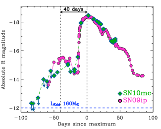
Figure 30.— The comparison of the absolute R band magnitude of SN 2009ip and Type IIn SN 2010mc (Ofek et al., 2013b) reveals a striking similarity between the two explosions both during the precursor-bump and the major outburst.

Our analysis characterizes the 2012b episode as a low-energy, asymmetric explosion happening in a complex medium, previously shaped by multiple episodes of shell ejection by the progenitor at different times. Here we address three major questions:

• What is the nature of the SN 2009ip double explosion in 2012?

• What is the underlying physical mechanism?

• What is the progenitor system of SN 2009ip?

We address the first two questions by considering the close similarity of SN 2009ip and SN 2010mc (Section 8.1), the properties of the progenitor system of SN 2009ip (Section 8.2), the physical mechanisms that can lead to sustained mass loss (Section 8.3) and the constraints on the energetics we derived from our modeling (Section 8.4).

8.1. SN 2009ip and SN 2010mc

In interpreting the fate and nature of SN 2009ip we have to consider its close likeness to SN 2010mc (Ofek et al., 2013b), the only other hydrogen-rich explosion with clear signs of interaction and a detected precursor before the major event. The similarity extends to the energetics, time scales (Fig. 30) and spectral properties both during the precursor bump and the major re-brightening, as noted by Smith et al. (2013).

The first important conclusion is that (i) the precursor and the major re-brightening are causally connected events, being otherwise difficult to explain the strictly similar phenomenology observed in SN 2009ip and SN 2010mc, two distinct and unrelated explosions. The same conclusion is independently supported by the very short time interval between the precursor and main outburst when compared to the progenitor star lifetime, as pointed out by Ofek et al. (2013b) for SN 2010mc. A second conclusion is that (ii) whatever causes the precursor plus major outburst phenomenology, this is not unique to SN 2009ip and might represent an important evolutionary channel for massive stars.

Furthermore, (iii) SN 2009ip and SN 2010mc must share some fundamental properties. In particular their evolution through the explosive phase must be driven by few physical parameters. A more complicated scenario would require unrealistic fine tuning to reproduce the close similarity of SN 2009ip and SN 2010mc. This also suggests we are sampling some fundamental step in the stellar evolution of the progenitor system. Finally, (iv) whatever the physical mechanism behind, the time interval of $\sim 40$ days (Fig. 30) between the precursor explosion and the main event must be connected to some physically important time scale for the system.

We employ the fast $\chi^{2}$ technique for irregularly sampled data by Palmer (2009) to search for periodicity and/or dominant time-scales in the outburst history of SN 2009ip before the major 2012 explosion. Details can be found in Appendix B. Applying the method above to the R-band data we find evidence for a dominant time-scale of $\sim 38$ days, (with significant power distributed on time-scales between 30 and 50 days), intriguingly similar to the $\Delta t\sim 40$ days between the precursor and major explosion in 2012. We emphasize that this is not a claim for periodicity, but the identification of a dominant variability time-scale of the signal.

Our analysis identifies the presence of a fundamental time-scale which regulates both the progenitor outburst history and the major explosion, and that is also shared by completely independent events like SN 2010mc. This time-scale corresponds to a tiny fraction of a massive star lifetime: $\sim 10^{-8}$ for $\tau\sim 4-6$ Myr, as appropriate for a $45-85\,\rm{M_{\sun}}$ star. We speculate on the nature of the underlying physical process in the next two sections.

8.2. The progenitor system of SN 2009ip

In Section 7.4 we showed that asymmetry plays a role in the 2012 explosion, which might point to the presence of a preferred direction in the progenitor system of SN 2009ip. This suggests either a (rapidly?) rotating single star or an interacting binary as progenitor for SN 2009ip. We first update previous estimates of the progenitor mass of SN 2009ip using the latest stellar evolutionary tracks and then discuss the effects of stellar rotation and the possibility of a binary progenitor.

From HST pre-explosion images, employing the latest Geneva stellar evolutionary tracks (Ekström et al., 2012) which include important updates on the initial abundances, reaction rates and mass loss prescriptions with respect to Schaller et al. (1992), we determine for $M_{\rm{V}}=-10.3\pm 0.3$ (Foley et al., 2011) a ZAMS mass $M\gtrsim 60\,\rm{M_{\sun}}$ assuming a non-rotating progenitor at solar composition, consistent with previous estimates. $M_{\rm{V}}=-10.3$ corresponds to $L_{\rm{V}}\sim 10^{6.1}L_{\rm{\sun}}$. This implies $L_{\rm{bol}}>2\times 10^{6}\,\rm{L_{\sun}}$, thus rivaling the most luminous stars ever discovered (e.g. Crowther et al. 2010). Luminosities of a few $10^{6}\,\rm{L_{\sun}}$ have been indeed associated to the group of LBV stars with typical temperature of $\sim 15000-25000\,\rm{K}$. Adopting this range of temperature results in $L_{\rm{bol}}\sim 5\times 10^{6}\,\rm{L_{\sun}}$, suggesting that any progenitor with $M<160\,\rm{M_{\rm{\sun}}}$ was super Eddington at the time of the HST observations. For $(2<L_{\rm{bol}}<5)\times 10^{6}\,\rm{L_{\sun}}$ the allowed mass range is $60\,\rm{M_{\sun}}<M_{\rm{ZAMS}}<300\,\rm{M_{\sun}}$ (e.g. Crowther et al. 2010). Including the effects of axial rotation results instead in a more constrained range of allowed progenitor mass: $45\,\rm{M_{\sun}}<M_{\rm{ZAMS}}<85\,\rm{M_{\sun}}$ (for $\Omega/\Omega_{\rm{crit}}=0.4$).

Rapid rotation strongly affects the evolution of massive stars, in particular by increasing the global mass-loss rate (e.g. Maeder & Meynet 2000). More importantly, Maeder (2002) showed that the mass loss in rapidly rotating massive stars does not remain isotropic, but it is instead enhanced at the polar regions, thus favoring bipolar stellar winds (e.g. Georgy et al. 2011, their Fig. 2). As a result, the formation of an asymmetric (peanut shaped) nebula around rapidly rotating stars is very likely. Additionally, rapid rotation can induce mechanical mass loss, resulting in some matter to be launched into an equatorial Keplerian disk. It is clear that any explosion/eruption of the central star will thus naturally occur in a non-isotropic medium, as we find for SN 2009ip. Rotation further leads to enhanced chemical mixing (e.g. Chatzopoulos et al. 2012; Yoon et al. 2012).

HST pre-explosion images cannot, however, exclude the presence of a compact companion. The massive progenitor of SN 2009ip might be part of a binary system and the repetitive episodes of eruption might be linked to the presence of an interacting companion. The close periastron passages of a companion star in an eccentric binary system has been invoked by Smith & Frew (2011) to explain the brightening episodes of $\eta$Car in 1838 and 1843. In the context of SN 2009ip, Levesque et al. (2012) discussed the presence of a binary companion, while Soker & Kashi (2013) suggested that the 2012b explosion was the result of a merger of two stars, an extreme case of binary interaction. A binary scenario was also proposed by Soker (2013) for the cosmic twin of SN 2009ip, SN 2010mc.

A binary system would have a natural asymmetry (i.e., the preferred direction defined by the orbital plane) and a natural time scale (i.e., the orbital period) as indicated by the observations. A possible configuration suggested to lead to substantial mass loss is that of a binary system made of a compact object (NS) closely orbiting around a massive, extended star (Chevalier 2012 and references therein). In this picture the mass loss is driven by the inspiral of the compact object in the common envelope (CE) evolution and the expansion velocity of the material is expected to be comparable to the escape velocity for the massive star. For $v\sim 1000\,\rm{km\,s^{-1}}$ and $M\sim 45-85\,M_{\sun}$ the radius of the extended star is $R_{*}<(1-2)\times 10^{12}\rm{cm}$ (where the inequality accounts for the fact that we used the ZAMS mass). In this scenario, the mass loss is concentrated on the orbital plane of the binary (Ricker & Taam 2012), offering a natural explanation for the observed asymmetry (Section 7.4). However, it remains unexplained how this mechanism would be able to launch material with $v\sim 10^{4}\,\rm{km\,s^{-1}}$ as observed during the 2012a episode (Mauerhan et al. 2013, Pastorello et al. 2012). A potential solution might be the presence of a high-velocity accretion disk wind.While the presence of a dominant time scale common to the eruptive and explosive phases makes the binary progenitor explanation particularly appealing, the common envelope model in its present formulation seems to have difficulties in explaining the observed phenomenology. Alternative scenarios are explored in Section 8.3.

8.3. Physical mechanisms leading to substantial mass loss in evolved single stars

The outer envelope of an evolved massive star contains $\sim 95\%$ of the stellar radius but only a tiny fraction of the stellar mass. The physical mechanism leading to the 2012a outburst must have been fairly deep seated to unbind more than $\sim 0.1\,\rm{M_{\sun}}$. It is furthermore required to generate a large amount of energy ($10^{48}$ erg plus the energy to lift the mass out of the deep gravitational potential well) and to explain the presence of a dominant time scale of $\sim 40$ days which is also shared with the observed eruption history in the years before the explosion. The mass-loss rate of at least a few $\sim 0.1\,\rm{M_{\sun}}/yr$ can only be sustained for an extremely small fraction of the life of a star and in principle only for $\sim$ years, before inducing important adjustments to the stellar structure. We explore here different physical mechanisms that have been proposed to lead to substantial mass loss in the late stages of evolution of massive single stars and discuss their relevance for SN 2009ip. They can basically be grouped into 4 categories: (i) pulsational pair-instability; (ii) super-Eddington fusion luminosity; (iii) Eddington-limit instabilities; (iv) shock heating of the stellar envelope.

Pulsational pair-instability (PPI, Barkat et al. 1967) applies to massive stars with helium core of $\sim 40-60\,\rm{M_{\sun}}$. PPI leads to partial unbinding of the star, with a sequence of eruptions accompanied by the ejection of shells of material of the stellar envelope. This mechanism has been considered as a plausible explanation for SN 2009ip by Pastorello et al. (2012), Mauerhan et al. (2013) and Fraser et al. (2013) but has been rejected by Ofek et al. (2013b) and Ofek et al. (2013a) for both SN 2010mc and SN 2009ip (the leading argument being that PPI would lead to the ejection of much larger amounts of mass than the $\sim 10^{-1}-10^{-2}\,\rm{M_{\sun}}$ they infer). According to Woosley et al. (2007), a non-rotating star with zero metallicity (Z=0) and ZAMS mass $95$ and $130\,\rm{M_{\sun}}$ meets the criteria for PPI. However, with updated prescriptions for the mass-loss rate, and assumption of solar metallicity (which more closely represents our conditions of $0.4\,\rm{Z_{\sun}}<Z<0.9\,\rm{Z_{\sun}}$, Section 5) Ekström et al. (2012) predict that even stars with $M=120\,\rm{M_{\sun}}$ will end the C-burning phase with mass $\sim 31\,\rm{M_{\sun}}$, below the threshold of $\sim 40\,\rm{M_{\sun}}$ to trigger PPI. While our limits on the progenitor mass of SN 2009ip in Sec. 8.2 do not formally rule out the PPI scenario in the non-rotating case, they definitely allow for progenitors starting with much lower mass than required for the PPI to develop ($M\gtrsim 120\,\rm{M_{\sun}}$).

Rapidly rotating progenitors ($\Omega/\Omega_{\rm{crit}}>0.5$) enter the PPI regime starting with substantially lower ZAMS mass: $\sim 50\,\rm{M_{\sun}}$ for $Z=0$ (Chatzopoulos & Wheeler 2012; Yoon et al. 2012). On the other hand, for $Z=Z_{\sun}$ even very massive rotating $120\,\rm{M_{\sun}}$ stars develop a core with $M\sim 19\,\rm{M_{\sun}}$, insufficient to trigger PPI (Ekström et al., 2012). In the previous sections we constrained the progenitor of SN 2009ip with ZAMS mass $45\,\rm{M_{\sun}}<M<85\,\rm{M_{\sun}}$ and metallicity $0.4\,\rm{Z_{\sun}}<Z<0.9\,\rm{Z_{\sun}}$. Following the prescriptions from Chatzopoulos & Wheeler (2012), adopting the most favorable conditions (i.e. $M=85\,\rm{M_{\sun}}$ and $Z=0.4\,Z_{\sun}$) and starting with a very rapidly rotating star with $\Omega/\Omega_{\rm{crit}}=0.9$, we find the final oxygen core mass to have $M\sim 35\,\rm{M_{\sun}}$, formally below the threshold of $40\,\rm{M_{\sun}}$ for PPI. This indicates some difficulties for rotating progenitors to reach the PPI threshold. What remains difficult to interpret both for rotating and non-rotating progenitors is the presence of a dominant time-scale of $\sim 40$ days: depending on the pulse properties and the physical conditions of the surviving star, the interval between pulses can be anywhere between days to decades (Woosley et al., 2007).

Alternatively, convective motions stimulated by the super-Eddington fusion luminosity in the core of a massive star can excite internal gravity waves (g-mode non-radial oscillations, Quataert & Shiode 2012). An important fraction of the energy in gravity waves can be converted into sound waves, with the potential to unbind several $M_{\sun}$. For a $40\,M_{\sun}$ star, Quataert & Shiode (2012) estimate that $10^{47}-10^{48}\,\rm{erg}$ will be deposited into the stellar envelope. If this mechanism is responsible for the ejection of material by the 2012a explosion, the velocity $v\sim 1000\,\rm{km\,s^{-1}}$ of the unbound material inferred from our observations implies an ejecta mass $\lesssim 0.1\,\rm{M_{\sun}}$, consistent with our estimate of the mass of the compact shell encountered by the 2012b explosion in Section 7.2. However, this mechanism is likely to lead to a steady mass-loss (E. Quataert private communication) as opposed to shell ejection and does not offer a natural explanation for the 40-day time scale involved in the process. We therefore consider the super-Eddington luminosity mechanism unlikely to apply to SN 2009ip and SN 2010mc, (see however Ofek et al. 2013b).

With $R$-band observed magnitudes between $\sim 18$ mag and $\sim 21$ mag reported by Pastorello et al. (2012), SN 2009ip oscillates between $\sim$Eddington and super-Eddington luminosity episodes in the years preceding the double explosion in 2012. Depending on the effective temperature of the emission, $R\sim 21$ mag corresponds to the Eddington luminosity of a star with mass $40-80\,\rm{M_{\sun}}$. $R\sim 18$ would correspond to an Eddington limit for a star of $M=600-1200\,\rm{M_{\sun}}$. A number of instabilities have been shown to develop in stars approaching and/or exceeding the Eddington limit, actually allowing the super-Eddington luminosity to persist (e.g. Owocki & Shaviv 2012), potentially powering LBV-like eruptions. The eruption time scale, repetition rate and ejected mass are however loosely predicted, so that it is unclear if any of these mechanisms would apply to the eruption history of SN 2009ip and, even more importantly, how these are connected with the 2012 double explosion (which clearly differs from super-Eddington powered winds). With luminosity between $\sim 10^{6}$ and $\sim 10^{7}\,\rm{L_{\sun}}$ the progenitor of SN 2009ip falls into the region where radiation pressure starts to have a major role in supporting the star against gravity (see e.g. Owocki & Shaviv 2012, their Fig. 12.1): we speculate that the dominance of radiation pressure over gas pressure in the envelope might have an important role in determining the repeated ejection of shells of SN 2009ip.

Indeed, the outer layers of massive stars close to the Eddington limit and/or critical rotation are only loosely bound and might be easily ejected if enough energy is suddenly deposited. A potential source of energy deposition has been identified in thermonuclear flashes associated with shell burning (Dessart et al., 2010). Differently from the PPI, this scenario does not require the progenitor to be extremely massive. Alternatively, non-radial gravity mode oscillations above the core or near to the H-burning shell could provide fresh fuel, triggering a burst of energy (and subsequent shell ejection) in massive stars like $\eta$Car (Guzik, 2005). Both scenarios have the advantage to be basically driven by two parameters: the deposited energy and the envelope binding energy, naturally satisfying the ”simplicity” criterion of Section 8.1.

Finally we mention that direct numerical simulations of pre-collapse hydrodynamics by Meakin (2006), Meakin & Arnett (2007) and Arnett & Meakin (2011a, b) found eruptive instabilities due to the interaction of oxygen and silicon burning shells. The instabilities are related to turbulent convection (and being inherently nonlinear, are invisible to conventional linear stability analysis). These simulations specifically predicted mass ejection prior to core collapse, suggesting that pre-collapse evolution is far more eventful than previously thought. However, as for all the other mechanisms analyzed in this section, it is at the moment unclear how to explain the 40-day time scale.

8.4. The nature of SN 2009ip double-explosion in 2012: the explosive ejection of the stellar envelope

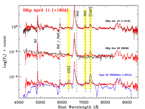
Figure 31.— Our spectrum taken in April 2013 ($t_{\rm{pk}}+190$ days) shows minimal evolution with respect to $\sim 100$ days before. The most notable difference with respect to spectra acquired after or during the LBV-like eruptions is the presence of intermediate He I and [CaII] in emission. We still do not find evidence for SN-synthesized material (e.g. [OI] 6300 Å ). We refer to Sahu et al. (2006) for details on Type IIP SN 2004et.

Our modeling shows that the 2012b explosion is not powered by Ni radioactive decay (Section 7.1) and demonstrates that a shock breaking out from a shell of material previously ejected by the 2012a outburst can reasonably account for the observed properties of the 2012b explosion, constraining the mass of the ejecta to $M_{\rm{ej}}=50.5(E/10^{51}\rm{erg})^{2}\,M_{\rm{\sun}}$ (Section 7.2). This strongly suggests an explosion energy well below $10^{51}\rm{erg}$ (likely around $10^{50}$ erg), and brings to question the fate of SN 2009ip: a terminal SN explosion (Mauerhan et al. 2013) or a SN ”impostor” (Pastorello et al. 2012; Fraser et al. 2013)?

A key prediction of the SN scenario is the presence of chemical elements produced by the SN nucleosynthesis (like oxygen) in late-time spectra, which is not expected in the case of a non-terminal explosion. Our latest spectrum acquired on 2013 April 11 ($t_{\rm{pk}}+190$ days) still shows no evidence for SN-synthesized material (Fig. 31). This non-detection is consistent with (but surely not a proof of) the non-terminal explosion scenario. This spectrum, dominated by H emission lines and where the high-velocity absorption features have completely disappeared, shares some similarities with pre-explosion spectra of SN 2009ip. A notable difference, however, is the presence of (intermediate width) He I and [Ca II]. The present data set therefore does not yet offer compelling evidence for a standard (i.e. resulting from the collapse of a degenerate core) SN-explosion scenario.

Interaction seems to be still dominating the emission at this time. Our late-time observations indicate a flattening in the light-curve (our latest V-band photometry acquired at $t_{\rm{pk}}+190$ days implies a decay of $\Delta V=+0.86\pm 0.22$ over 98.5 days, or $0.0087\pm 0.0022\,\rm{mag/day}$), which might be caused by the interaction of the shock with the NIR emitting material. Our model predicts that the “flat” phase should be followed by a rapid decline, once the shock has reached the edge of the “NIR shell”.

We propose that SN 2009ip was the consequence of the explosive ejection of the envelope of a massive star, which later interacted with shells of material ejected during previous eruption episodes. While $E<10^{51}\rm{erg}$ is insufficient to fully unbind a massive star, its outer envelope is only loosely bound, and can be easily ejected by a lower-energy explosion. The origin of the energy deposition is not constrained as unclear is its potential relation with the possible binary nature of the system. The final fate of SN 2009ip depends on the properties of the remaining “core”, and in particular, on its mass and rotation rate: if the star managed to explode its entire H envelope still retaining a super-critical core mass, it might re-explode in the future as a genuine H-poor (Ib/c) SN explosion; if instead the star partially retained its envelope, it will possibly give rise to other SN-impostor displays, on time scales which are difficult to predict.. The core might also have directly collapsed to a black hole: in this case this would mark the “end”. Only close inspection of the explosion site after SN 2009ip has appreciably faded will reveal if the star survived the ejection of its outer layers. Given the impressive similarity with SN 2010mc, our interpretation extends to this event as well.

9. Summary and Conclusions

The “2012 double-explosion” of SN 2009ip brought to light the limits of our current understanding of massive star evolution, pointing to the existence of new channels for sustained mass-loss in evolved stars, whose origins has still to be identified. Our extensive follow-up campaign and modeling allow us to identify the properties of a complex ejecta structure and an explosion environment shaped by repeating outbursts during the previous years. We find that:

• SN 2009ip is embedded in a sub-solar metallicity environment ($0.4\,Z_{\sun}<Z<0.9\,Z_{\sun}$) in the outskirts of its host galaxy ($d\sim 5$ kpc), radiated $\sim 3\times 10^{49}$ erg during the 2012b explosion, reaching a peak luminosity of $\sim 2\times 10^{43}\,\rm{erg\,s^{-1}}$. The 2012a precursor bump released $\sim 2\times 10^{48}$ erg.

• The explosion is not powered by ${}^{56}\rm{Ni}$ radioactive decay. From late-time photometry, the total ${}^{56}\rm{Ni}$ mass is $M_{\rm{Ni}}<0.08\,\rm{M_{\sun}}$. Narrow emission lines in the optical spectra require interaction of the explosion shock with the CSM at some level. We suggest this interaction is also responsible for mediating the conversion of the shock kinetic energy into radiation, powering the observed light-curve.

• Spectroscopy at optical to NIR wavelengths further identifies three distinct velocity components in the ejecta with $v\sim 12000\,\rm{km\,s^{-1}}$, $v\sim 5500\,\rm{km\,s^{-1}}$ and $v\sim 2500\,\rm{km\,s^{-1}}$, arguing against a continuous velocity distribution. No departure from spherical symmetry needs to be invoked for the slow-moving ($v\leq 5500\,\rm{km\,s^{-1}}$) ejecta. Instead, spherical symmetry is clearly broken by the high-velocity material, possibly pointing to the presence of a preferred direction in the explosion. Broad and intermediate components in the optical/NIR spectra are consistent with the view that asymmetry might also have a role in the spatial distribution of the interacting material.

• CSM material in the region surrounding SN 2009ip, with a velocity of a few to several $100\,\rm{km\,s^{-1}}$, originates from abrupt episode(s) of mass ejection in the previous years. Mass loss is unlikely to have occurred in the form of a steady wind: instead, our analysis favors explosive mass ejections, likely linked to instabilities developing deep inside the stellar core.

• We interpret the major 2012 re-brightening to be caused by the explosion shock breaking out through a compact and dense CSM shell previously ejected in the 2012a outburst. Our analysis constrains the onset of the explosion to be $\sim 20$ days before peak. The break-out radius is $R_{\rm{bo}}\sim 5\times 10^{14}\rm{cm}$. The shell extends to $R_{\rm{w}}\sim 1.2\times 10^{15}\rm{cm}$, with a total mass of $M_{\rm{w}}\sim 0.1\,\rm{M_{\sun}}$. The presence of a compact and dense shell is independently supported by (i) the detection of X-ray radiation with $L_{\rm{x}}/L_{\rm{opt}}<10^{-4}$ and (ii) by the late-time rise of radio emission. After break-out the optical-UV light-curve is powered by continued interaction with optically thin material characterized by a steep density profile.

• A shock breaking out through a dense shell is expected to produce hard X-rays with a typical energy of 60 keV. We report a tentative detection of hard X-rays (15-150 keV range) around the optical peak and put a solid upper limit on the hard X-ray to optical emission from SN 2009ip: $L_{\rm{X,hard}}/L_{\rm{bol}}<5\times 10^{-3}$.

• The collision of the ejecta with a massive shell(s) is expected to accelerate cosmic rays and generate GeV gamma-rays. Using Fermi-LAT data we detect no GeV radiation, consistent with the picture of ejecta crashing into a compact and dense but low-mass shell of material at small radius.

• Our calculations indicate that the latest outburst from SN 2009ip was a bright source of neutrinos if the CR energy is comparable to the radiated energy. We demonstrate with SN 2009ip how to constrain the cosmic-ray acceleration efficiency using broad band electromagnetic data and deep limits on muon neutrinos that will be available in the near future when new facilities will come online.

• We speculate that the NIR excess of emission is a signature of vaporization of dust grains with radius $(2-5)\rm{\mu m}$ in a shell of material located at $R>4\times 10^{15}\rm{cm}$. The very high temperature associated with the NIR excess remains however difficult to explain. The shell was ejected by the progenitor in the years preceding 2012, and will be overtaken by the explosion shock during 2013.

• Finally, our modeling of the 2012b explosion implies a small ejecta mass $M_{\rm{ej}}\sim 0.5\,\rm{M_{\sun}}$, with an explosion energy well below $10^{51}$ erg (likely around $10^{50}$ erg), thus raising questions about the nature of SN 2009ip: was it a terminal SN explosion or a SN impostor?

This analysis constrains the 2012b re-brightening of SN 2009ip to be a low-energy, asymmetric explosion in a complex medium. We interpret this 2012b episode to be the explosive ejection of the envelope of the massive progenitor star that later interacted with shells of material ejected during previous eruption episodes.

To unravel the nature of the physical mechanism behind the complex phenomenology of SN 2009ip, two key observational findings stand out: (i) its extreme similarity with SN 2010mc both in terms of time scales and energetics of the precursor bump and main explosion; (ii) the presence of a dominant time scale of $\sim 40$ days, which regulates both the progenitor outburst history and major explosion (and which is also shared by completely independent events like SN 2010mc). While it is clear that the physical process leading to the 2012a eruption must have been fairly deep-seated to unbind $\sim 0.1\,\rm{M_{\sun}}$, it is unclear if any of the proposed mechanisms for substantial episodic mass loss (i.e. pulsational pair instability, super-Eddington fusion luminosity, Eddington-limit instabilities and shock heating of the stellar envelope) would be able to fully account for the observed properties, and in particular for the presence of dominant time scales. Indeed, the presence of dominant time scales might suggest a binary progenitor.

Finally, the extreme similarity to SN 2010mc allows us to conclude that the mechanism behind the precursor plus major outburst is not unique to SN 2009ip and is likely driven by few physical parameters. Moreover, this eruptive dynamic might represent an important evolutionary channel for massive stars. Future observations will reveal if SN 2009ip was able to survive.

Appendix A Shock break-out in a dense wind shell: direct constraints from observables

We provide here the set of equations we used to constrain the ejecta mass $M_{\rm{ej}}$, energy of the explosion $E$, the environment density $\rho_{\rm{w}}$ and mass-loss rate $\dot{M}$, starting from three observables: the radiated energy at break-out $E_{\rm{rad}}$, the bolometric light-curve rise-time $t_{\rm{rise}}$ and the radius at shock break-out $R_{\rm{bo}}$. This work is based on Chevalier & Irwin (2011) . We consider here their model (a) (see their Fig. 1), where the break-out happens inside the dense wind shell of radius $R_{\rm{w}}$ so that $R_{\rm{bo}}<R_{\rm{w}}$. For SN 2009ip it turns out that $R_{\rm{bo}}\lesssim R_{\rm{w}}$ which leads to comparable estimates of the explosion and the environment parameters even if one were to use their model (b). The density in the wind shell is $\rho_{\rm{w}}=\dot{M}/(4\pi r^{2}v_{\rm{w}})$, or $\rho_{\rm{w}}=Dr^{-2}$ with $D\equiv 5.0\times 10^{16}(\rm{g/cm})D_{*}$ and $r$ is in cgs units. We follow the parametrization by Chevalier & Irwin (2011) and solve their Eq. 1, Eq. 3 and Eq. 5 for the three observables. The system of equation is degenerate for $M_{\rm{ej}}/E^{2}$. We obtain:

$$M_{\rm{ej}}=10\Big{(}\frac{R_{\rm{bo}}}{4.0\times 10^{14}\rm{cm}}\Big{)}^{-2}\Big{(}\frac{E_{\rm{rad}}}{0.44\times 10^{50}\rm{erg}}\Big{)}^{-1}\Big{(}\frac{t_{\rm{rise}}}{6.6\,\rm{days}}\Big{)}^{2}\Big{(}\frac{E}{10^{51}\rm{erg}}\Big{)}^{2}M_{\sun}$$ (A1)

$$D_{*}=\Big{(}\frac{t_{\rm{rise}}}{6.6\,\rm{days}}\Big{)}^{2}\Big{(}\frac{R_{\rm{bo}}}{4.0\times 10^{14}\rm{cm}}\Big{)}^{-3}\Big{(}\frac{E_{\rm{rad}}}{0.44\times 10^{50}\rm{erg}}\Big{)}$$ (A2)

$$\dot{M}=D_{*}\Big{(}\frac{v_{\rm{w}}}{1000\,\rm{km\,s^{-1}}}\Big{)}\rm{M_{\sun}yr^{-1}}$$ (A3)

$$k=0.34\Big{(}\frac{R_{\rm{bo}}}{4.0\times 10^{14}\rm{cm}}\Big{)}^{3}\Big{(}\frac{E_{\rm{rad}}}{0.44\times 10^{50}\rm{erg}}\Big{)}^{-1}\Big{(}\frac{t_{\rm{rise}}}{6.6\,\rm{days}}\Big{)}^{-1}\rm{cm^{2}/g}$$ (A4)

where $v_{\rm{w}}$ is the wind velocity and $k$ is the opacity. The mass of the wind shell enclosed within a radius $R$ is:

$$M_{\rm{w}}(r<R)=6.3\times 10^{17}\Big{(}\frac{R}{\rm{cm}}\Big{)}\Big{(}\frac{t_{\rm{rise}}}{6.6\,\rm{days}}\Big{)}^{2}\Big{(}\frac{R_{\rm{bo}}}{4.0\times 10^{14}\rm{cm}}\Big{)}^{-3}\Big{(}\frac{E_{\rm{rad}}}{0.44\times 10^{50}\rm{erg}}\Big{)}\rm{g}$$ (A5)

The luminosity from continued shock -wind interaction (Chevalier & Irwin 2011, their Eq. 9) after break-out can be written as:

$$L(t)=7.1\times 10^{43}\Big{(}\frac{E_{\rm{rad}}}{0.44\times 10^{50}\rm{erg}}\Big{)}\Big{(}\frac{t_{\rm{rise}}}{6.6\,\rm{days}}\Big{)}^{-0.4}\Big{(}\frac{t}{10\,\rm{days}}\Big{)}^{-0.6}\rm{erg\,s^{-1}}$$ (A6)

The radius of the wind shell is:

$$R_{\rm{w}}=8.3\times 10^{13}\Big{(}\frac{t_{\rm{rise}}}{6.6\,\rm{days}}\Big{)}^{-0.8}\Big{(}\frac{R_{\rm{bo}}}{4.0\times 10^{14}\rm{cm}}\Big{)}\Big{(}\frac{t_{\rm{w}}}{\rm{days}}\Big{)}\rm{cm}$$ (A7)

where $t_{\rm{w}}$ is the time when the shock reaches the edge of the shell. In this scenario, the onset of the explosion is at:

$$t_{0}\approx t_{\rm{peak}}-2t_{\rm{rise}}$$ (A8)

Assuming hydrogen rich material with $\langle\mu_{\rm{p}}\rangle=1$, the column density from radius $R$ to the observer can be written as (see Ofek et al. 2013a):

$$N(R)\approx 3.02\times 10^{25}\Big{(}\frac{t_{\rm{rise}}}{6.6\,\rm{days}}\Big{)}^{2}\Big{(}\frac{R_{\rm{bo}}}{4.0\times 10^{14}\rm{cm}}\Big{)}^{-3}\Big{(}\frac{E_{\rm{rad}}}{0.44\times 10^{50}\rm{erg}}\Big{)}\Big{(}\frac{R}{10^{15}\,\rm{cm}}\Big{)}^{-1}\rm{cm^{-2}}$$ (A9)

The bound-free optical depth at radius $R$ as a function of the energy of the photons, $E$ is $\tau_{\rm{bf}}=N\sigma(E)$ or

$$\tau_{\rm{bf}}(E)\approx 3\times 10^{3}\Big{(}\frac{t_{\rm{rise}}}{6.6\,\rm{days}}\Big{)}^{2}\Big{(}\frac{R_{\rm{bo}}}{4.0\times 10^{14}\rm{cm}}\Big{)}^{-3}\Big{(}\frac{E_{\rm{rad}}}{0.44\times 10^{50}\rm{erg}}\Big{)}\Big{(}\frac{R}{10^{15}\,\rm{cm}}\Big{)}^{-1}\Big{(}\frac{E}{\rm{keV}}\Big{)}^{-2.5}$$ (A10)

adopting the approximated cross-section as in Ofek et al. (2013a). The free-free optical depth $\tau_{\rm{ff}}$ at radius $R$ as a function of photon frequency $\nu$ is:

$$\tau_{\rm{ff}}(\nu)\approx 2.6\times 10^{8}\Big{(}\frac{T_{e}}{10^{4}\,\rm{K}}\Big{)}^{-1.35}\Big{(}\frac{\nu}{\rm{GHz}}\Big{)}^{-2.1}\Big{(}\frac{R}{10^{15}\,\rm{cm}}\Big{)}^{-3}\Big{(}\frac{t_{\rm{rise}}}{6.6\,\rm{days}}\Big{)}^{4}\Big{(}\frac{R_{\rm{bo}}}{4.0\times 10^{14}\rm{cm}}\Big{)}^{-6}\Big{(}\frac{E_{\rm{rad}}}{0.44\times 10^{50}\rm{erg}}\Big{)}^{2}$$ (A11)

where $T_{e}$ is the electron temperature.

Appendix B Temporal Analysis

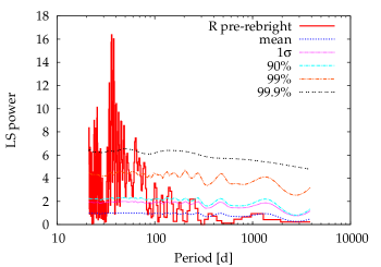
Figure 32.— Lomb-Scargle periodogram of the R-band magnitude time series for the time interval August 2009 - April 2012 (i.e. before the 2012a and 2012b explosions). This plot shows significant power on time-scales around $\sim 40$ days. We emphasize that this is not a claim for periodicity. Contours at various significance levels are also shown.

We identify the presence of a dominant time-scale of $\sim 40$ days by applying the the Fast $\chi^{2}$ algorithm developed by Palmer (2009) to the R-band photometry obtained for SN 2009ip by Pastorello et al. (2012) in the period August 2009 - April 2012. This algorithm is suitable for irregularly sampled data with nonuniform errors and it is designed to identify the presence of periodic signals by minimizing the $\chi^{2}$ between the data and the model. We adopt a linear model for the trend. The best period was found to be $T_{0}=115$ days. However, the reduction in the $\chi^{2}$ obtained for this period is comparable over a broad range of period candidates, thus proving that there it is no periodic or quasi–periodic signal. Assuming the Fourier decomposition with the fundamental period $T_{0}$, among the first seven harmonics most (52%) of the temporal power is carried by the third harmonic ($T_{0}/3=38$ days), followed by the fundamental (19%), the fifth harmonic ($T_{0}/5=23$ days, 10%), the second and fourth harmonics ($T_{0}/2=58$ and $T_{0}/4=29$ days, 5% each). This is evidence for a dominant time-scale of about 40 days, with significant power distributed on time-scales between 30 and 50 days. Replicating the same analysis on time series obtained by randomizing the observed magnitudes has the effect of washing out the excess of power on those time scales. This demonstrates that the excess of power around 40 days is not due to the data sampling.

Additionally and independently, we calculated the Lomb–Scargle (LS; Lomb 1976; Scargle 1982) periodogram of the same time series. This is particularly suitable to unevenly sampled data sets and measures the power contributed by the different frequencies to the total variance. This reduces to the Fourier power spectrum in the uniform sampling limit. As shown in Fig. 32, most power is concentrated between $\sim 30$ and $\sim$50 days, with a peak around 40 days. To evaluate the impact of the aliasing and to quantify how significant the power is with respect to the white noise case (i.e. no preferred time scale), we carried out the following Monte Carlo simulation. We randomized the magnitudes among the same observation times and generated $10^{4}$ synthetic profiles with the same variance as the real one. For each period we derived the corresponding confidence levels of $1\sigma$, 90%, 99%, and 99.9%, as shown in Fig. 32. Comparing the real LS periodogram with the MC generated confidence levels, we conclude that power in excess of white noise around 40 days is significant at 99.9% confidence and we identify this time scale as the dominant one in the overall variance.

In addition, we applied both methods to the time profiles obtained for the V, H and R filters around the 2012 outburst. We applied both a third and a fourth degree polynomial de-trending. In all cases, we obtained similar results with dominant time scales in the range 30–50 days. This is a robust result which does not crucially depend on the polynomial degree used for de-trending the series.

Appendix C Observing Logs

Table 2Log of observed Swift-UVOT spectra

Date (UT)	Time range (UT)	Obs ID	Exposure (ks)	Roll Angle
2012-09-27	09:03:41-14:37:27	31486008	5.1	212.0
2012-09-28	13:41:01-16:53:23	31486011	3.4	215.0
2012-09-29	10:27:52-12:24:46	31486012	3.3	215.0
2012-09-30	05:48:22-17:19:31	32570001	4.9	216.0
2012-10-01	01:13:23-19:11:08	32570002	4.0	216.0
2012-10-02	14:08:21-22:05:35	31486020	5.3	229.0
2012-10-03	02:49:01-15:52:51	32570003	4.4	220.0
2012-10-04	09:10:01-14:19:17	32570004	5.1	220.0
2012-10-05	09:12:55-15:33:06	32570005	7.2	220.0
2012-10-06	04:26:57-11:09:55	32570006	6.7	220.0
2012-10-07	07:41:54-08:05:27	32570007	6.2	220.0
2012-10-08	07:44:55-12:57:21	32579001	6.2	243.0
2012-10-10	03:01:55-12:56:01	32579002	6.5	243.0
2012-10-12	06:20:54-11:31:19	32579003	5.7	243.0
2012-10-14	04:50:54-06:54:14	32579004	5.8	243.0
2012-10-16	06:32:56-11:35:19	32579005	5.7	243.0
2012-10-20	08:30:16-13:41:40	32579007	5.3	243.0
2012-10-22	09:59:14-13:30:15	32579008	3.5	243.0
2012-10-24	13:19:14-17:00:26	32605001	4.3	249.0
2012-10-26	10:10:14-13:53:54	32605002	3.7	249.0
2012-10-28	08:41:21-09:00:03	32605003	1.1	249.0
2012-11-02	17:09:16-19:03:52	32605004	11.3	249.0

Table 3Log of observed optical spectra

Date (UT)	Telescope/Inst.	Range (Å)	R ($\lambda/\Delta\lambda$)	Grating (l/mm)	Aperture (arcsec)	Airmass	Exp. Time (s)
Aug 26.83	SALT/RSS	3500$-$10000	300	300	1.25	2.84	900
Sep 26.75	SALT/RSS	3500$-$10000	300	300	1.25	1.16	1200
Sep 27.99	Magellan/MagE	3150.0$-$9400.0	3400	175	1.5	1.25	600
Sep 28.99	Magellan/MagE	3150$-$9400	3400	175	1.5	1.23	1200
Sep 30.02	VLT/X-shooter	3000$-$25000	5100$-$8800	–	1.0/0.9/0.9	1.10	744/556/800c
Oct 11.15	KPNO/RCSpec	3080$-$8760	1200	316	1.5	2.15	1200
Oct 11.93	SALT/RSS	3500$-$10000	300	300	1.25	1.24	300
Oct 12.16	KPNO/RCSpec	3080$-$8760	1200	316	1.5	2.09	1200
Oct 12.94	SALT/RSS	3500$-$10000	300	300	1.25	1.29	300
Oct 13.16	KPNO/RCSpec	5380$-$8290	2500	632	1.5	2.07	6000
Oct 13.18	FLWO/FAST	3470$-$7414	2700	300	3.0	2.04	1800
Oct 14.15	KPNO/RCSpec	5380$-$8290	2500	632	1.5	2.10	3600
Oct 14.17	MMT/Blue Channel	3350$-$8570	1200	300	1.0	2.03	300
Oct 14.18	MMT/Blue Channel	5860$-$7160	5000	1200	1.0	2.03	600
Oct 14.21	MMT/Blue Channel	3800$-$5120	3000	1200	1.0	2.12	900
Oct 14.21	FLWO/FAST	3469$-$7413	2700	300	3.0	2.07	1800
Oct 15.21	FLWO/FAST	3473$-$7417	2700	300	3.0	2.08	1800
Oct 15.14	KPNO/RCSpec	5380$-$8290	2500	632	1.5	2.11	4800
Oct 15.14	MMT/Blue Channel	3350$-$8570	1200	300	1.0	2.03	300
Oct 16.19	FLWO/FAST	3472$-$7416	2700	300	3.0	2.05	1500
Oct 17.19	FLWO/FAST	3474$-$7418	2700	300	3.0	2.04	1602
Oct 20.25	FLWO/FAST	3481$-$7422	2700	300	3.0	2.20	1500
Oct 21.25	FLWO/FAST	3475$-$7419	2700	300	3.0	2.80	1500
Oct 22.18	FLWO/FAST	3474$-$7418	2700	300	3.0	2.04	1500
Oct 23.90	SALT/RSS	3200-9000	1500	900	1.25	1.20	600
Oct 27.89	SALT/RSS	3200-9000	1500	900	1.25	1.21	600
Oct 31.13	VLT/X-shooter	3000$-$25000	5100$-$8800	–	1.0/0.9/0.9c	1.23	744/556/800c
Nov 10.85	SALT/RSS	3300$-$10500	300	300	1.25	1.25	600
Nov 14.06	MMT/Blue Channel	3320$-$8540	1200	300	1.0	2.11	900
Nov 14.08	MMT/Blue Channel	5840$-$7140	5000	1200	1.0	2.06	1000
Nov 14.11	MMT/Blue Channel	3780$-$5110	3000	1200	1.0	2.04	1500
Nov 17.04	Magellan/IMACS	4200 - 9300	1300	300	0.7	1.02	2700
Nov 23.81	SALT/RSS	3200 - 9000	1500	900	1.25	1.25	600
Dec 05.01	Magellan/IMACS	3500 - 9400	1300	300	0.7	1.25	27000
Dec 14.04	SOAR/GHTS	3930 - 7985	300	1390	0.84	1.44	1800
Dec 21.07	MMT/Blue Channel	3300 - 8500	300	740	1.0	2.46	2000
Jan 12.04	Magellan/LDSS3	3780$-$10500	650	VPH-all	1.0	2.75	1200
Apr 11.39	Magellan/IMACS	4000$-$10200	1600	300	0.9	1.87	1200

Table 4Log of observed NIR spectra

Date (UT)	Inst.	Range (Å)	R ($\lambda/\Delta\lambda$)	Grating (l/mm)	Aperture (arcsec)	Airmass	Exp. Time (s)
Sep 27.21	MDM	9700 $-$ 18000	720	$\cdots$	0.7	2.00	1600
Sep 29.19	MDM	9700 $-$ 24300	720	$\cdots$	0.7	2.00	1600
Sep 30.20	MDM	9700 $-$ 24300	720	$\cdots$	0.7	2.00	1600
Nov 05.11	FIRE	8000 $-$ 27400	500	$\cdots$	0.6	1.24	761
Nov 19.09	FIRE	8200 $-$ 25000	6000		0.6	1.28	1200
Nov 25.11	FIRE	8000 $-$ 27200	500	$\cdots$	0.6	1.67	1014
Dec 03.04	FIRE	8000 $-$ 27200	500	$\cdots$	0.6	1.31	1014

Appendix D Photometry Tables

Table 5Swift-UVOT photometry

Date	v	Date	b	Date	u	Date	w1	Date	w2	Date	m2
(d)	(mag)	(d)	(mag)	(d)	(mag)	(d)	(mag)	(d)	(mag)	(d)	(mag)
84.68	20.50(0.30)	84.68	20.76(0.19)	84.68	20.08(0.17)	84.67	20.48(0.19)	84.68	20.77(0.17)	84.69	20.87(0.23)
1174.88	17.10(0.21)	1174.90	17.29(0.05)	1174.90	16.48(0.06)	1174.89	17.09(0.07)	1174.90	17.85(0.09)	1176.64	17.73(0.09)
1176.64	17.52(0.15)	1176.64	17.24(0.07)	1176.64	16.46(0.07)	1176.63	16.96(0.08)	1176.64	17.86(0.10)	1183.44	18.92(0.12)
1183.44	17.74(0.15)	1183.44	17.62(0.08)	1183.44	17.23(0.09)	1183.43	18.08(0.11)	1183.44	19.09(0.14)	1192.74	20.25(0.22)
1192.77	18.16(0.10)	1190.75	18.39(0.15)	1190.75	17.77(0.12)	1190.75	19.08(0.21)	1192.77	20.31(0.18)	1196.35	12.78(0.04)
1196.24	14.91(0.05)	1192.76	18.13(0.06)	1192.76	17.88(0.07)	1192.76	19.23(0.16)	1196.34	12.83(0.05)	1198.48	12.30(0.04)
1196.31	14.95(0.05)	1196.23	14.81(0.05)	1196.23	13.46(0.05)	1196.34	12.98(0.04)	1197.46	12.66(0.05)	1200.99	12.10(0.04)
1196.37	14.86(0.05)	1196.30	14.75(0.05)	1196.30	13.44(0.05)	1197.47	12.75(0.04)	1197.71	12.52(0.05)	1201.99	12.12(0.04)
1196.45	14.83(0.05)	1196.36	14.77(0.05)	1196.36	13.39(0.05)	1197.70	12.62(0.04)	1198.48	12.42(0.04)	1202.75	12.17(0.04)
1198.48	14.38(0.04)	1196.45	14.74(0.05)	1196.45	13.36(0.05)	1198.47	12.51(0.04)	1198.59	12.43(0.04)	1202.26	12.14(0.04)
1199.66	14.26(0.05)	1197.70	14.39(0.05)	1197.70	12.99(0.05)	1198.61	12.59(0.04)	1199.65	12.32(0.04)	1203.07	12.13(0.04)
1200.99	14.14(0.05)	1198.48	14.28(0.04)	1198.47	12.90(0.04)	1199.47	12.53(0.04)	1200.99	12.20(0.04)	1204.06	12.06(0.04)
1201.99	14.07(0.05)	1199.65	14.11(0.05)	1199.65	12.78(0.04)	1199.65	12.41(0.04)	1201.99	12.19(0.04)	1206.13	12.04(0.04)
1202.26	14.11(0.05)	1200.98	13.94(0.05)	1200.98	12.65(0.04)	1200.98	12.30(0.04)	1201.38	12.23(0.04)	1208.68	12.30(0.04)
1203.06	14.10(0.05)	1201.98	13.98(0.05)	1201.98	12.61(0.04)	1201.98	12.31(0.04)	1202.26	12.21(0.04)	1210.07	12.47(0.04)
1204.05	13.91(0.05)	1202.25	13.96(0.05)	1200.47	12.72(0.04)	1202.25	12.31(0.04)	1203.06	12.23(0.04)	1212.20	12.58(0.04)
1206.13	13.88(0.05)	1203.06	13.96(0.05)	1202.25	12.64(0.04)	1203.06	12.30(0.04)	1200.49	12.26(0.04)	1214.14	12.71(0.04)
1208.67	13.92(0.05)	1203.32	13.96(0.05)	1203.06	12.63(0.04)	1204.05	12.22(0.04)	1201.43	12.23(0.04)	1216.21	13.16(0.04)
1210.06	13.88(0.05)	1204.05	13.84(0.05)	1203.12	12.67(0.04)	1206.12	12.17(0.04)	1203.27	12.27(0.04)	1216.41	13.20(0.06)
1212.20	13.95(0.05)	1204.52	13.76(0.13)	1203.32	12.63(0.06)	1208.67	12.44(0.04)	1204.05	12.16(0.04)	1218.83	13.88(0.04)
1214.14	13.93(0.05)	1205.52	13.73(0.11)	1203.39	12.67(0.06)	1210.06	12.55(0.04)	1204.50	12.13(0.04)	1220.55	14.22(0.04)
1216.21	14.13(0.05)	1206.12	13.75(0.05)	1204.05	12.60(0.04)	1212.20	12.69(0.04)	1205.53	12.13(0.04)	1222.29	14.49(0.04)
1218.83	14.30(0.05)	1208.67	13.86(0.05)	1204.38	12.56(0.04)	1214.13	12.77(0.04)	1206.12	12.14(0.04)	1222.41	14.49(0.05)
1220.55	14.30(0.05)	1210.06	13.91(0.05)	1205.38	12.57(0.04)	1218.82	13.71(0.04)	1206.33	12.18(0.04)	1224.49	14.82(0.04)
1222.29	14.43(0.05)	1212.20	13.91(0.05)	1205.52	12.54(0.04)	1220.55	13.95(0.04)	1208.67	12.47(0.04)	1226.49	15.20(0.05)
1224.49	14.46(0.05)	1214.14	13.97(0.05)	1205.65	12.56(0.04)	1222.28	14.18(0.04)	1207.44	12.30(0.04)	1226.23	15.16(0.05)
1226.23	14.75(0.06)	1216.27	14.18(0.07)	1206.12	12.50(0.04)	1224.49	14.40(0.04)	1208.44	12.45(0.04)	1228.71	15.64(0.05)
1228.71	15.01(0.06)	1218.83	14.39(0.05)	1206.25	12.51(0.04)	1226.23	14.75(0.05)	1210.34	12.70(0.04)	1230.38	15.92(0.06)
1230.38	15.23(0.07)	1220.55	14.44(0.05)	1208.39	12.63(0.04)	1228.70	15.30(0.05)	1210.06	12.65(0.04)	1232.86	16.21(0.06)
1232.86	15.09(0.06)	1222.29	14.57(0.05)	1208.52	12.60(0.06)	1230.37	15.48(0.06)	1212.20	12.80(0.04)	1234.41	16.21(0.05)
1233.98	14.85(0.09)	1224.49	14.68(0.05)	1208.52	12.61(0.04)	1232.85	15.64(0.06)	1214.14	12.94(0.04)	1234.98	16.18(0.08)
1234.98	14.86(0.09)	1226.23	14.94(0.05)	1208.67	12.63(0.04)	1234.48	15.52(0.06)	1216.21	13.44(0.04)	1236.18	16.13(0.06)
1236.21	14.95(0.05)	1228.71	15.25(0.06)	1210.06	12.80(0.04)	1236.21	15.53(0.05)	1216.47	13.50(0.04)	1238.09	16.31(0.05)
1238.09	15.16(0.05)	1230.37	15.50(0.06)	1210.19	12.75(0.04)	1238.08	15.72(0.05)	1218.83	14.22(0.04)	1240.06	16.58(0.06)
1240.06	15.34(0.06)	1232.85	15.38(0.06)	1210.46	12.75(0.04)	1240.09	16.01(0.05)	1212.38	12.82(0.04)	1242.30	16.93(0.06)
1242.29	15.68(0.06)	1234.48	15.16(0.06)	1212.20	12.76(0.04)	1242.29	16.27(0.05)	1214.25	12.97(0.04)	1242.30	16.93(0.06)
1244.43	15.88(0.06)	1236.18	15.25(0.06)	1212.33	12.78(0.06)	1244.46	16.63(0.09)	1216.39	13.47(0.04)	1244.43	17.28(0.07)
1246.91	16.00(0.06)	1238.08	15.40(0.05)	1212.33	12.80(0.04)	1246.93	16.94(0.08)	1220.47	14.59(0.04)	1246.94	17.39(0.08)
1248.05	15.83(0.06)	1240.05	15.73(0.05)	1212.46	12.81(0.04)	1248.04	16.88(0.07)	1222.50	14.84(0.04)	1248.05	17.57(0.07)
1250.05	16.04(0.07)	1242.29	16.07(0.05)	1214.14	12.84(0.04)	1250.04	17.05(0.08)	1220.55	14.58(0.04)	1250.05	17.85(0.08)
1252.59	16.17(0.07)	1244.46	16.23(0.08)	1216.20	13.09(0.04)	1252.59	17.34(0.08)	1222.29	14.86(0.04)	1252.59	18.32(0.10)
1254.09	16.33(0.06)	1246.91	16.42(0.06)	1216.27	13.05(0.06)	1254.09	17.50(0.07)	1224.49	15.19(0.05)	1254.09	18.32(0.08)
1256.70	16.32(0.09)	1248.04	16.33(0.06)	1216.27	13.07(0.04)	1256.66	17.83(0.09)	1226.23	15.54(0.06)	1256.70	18.57(0.13)
1258.53	16.42(0.07)	1250.01	16.47(0.07)	1216.40	13.06(0.06)	1258.52	17.93(0.09)	1224.64	15.21(0.04)	1258.54	18.78(0.10)
1260.34	16.45(0.07)	1252.59	16.80(0.06)	1216.41	13.09(0.04)	1260.33	18.04(0.09)	1226.44	15.56(0.06)	1260.34	18.65(0.09)
1262.21	16.41(0.06)	1254.09	16.85(0.06)	1218.82	13.48(0.04)	1262.20	18.42(0.11)	1228.71	16.10(0.06)	1262.21	18.95(0.11)
1264.61	16.60(0.07)	1256.66	17.00(0.06)	1220.55	13.66(0.04)	1264.60	18.32(0.11)	1230.37	16.32(0.06)	1264.61	18.99(0.12)
1266.15	16.71(0.07)	1258.53	17.16(0.06)	1220.45	13.69(0.04)	1266.14	18.41(0.11)	1232.86	16.55(0.06)	1266.15	19.28(0.13)
1268.66	17.00(0.08)	1260.30	17.20(0.08)	1222.29	13.75(0.04)	1268.66	18.73(0.13)	1233.79	16.48(0.05)	1268.66	19.43(0.14)
1270.35	17.28(0.10)	1262.20	17.11(0.06)	1224.62	14.02(0.04)	1270.34	18.70(0.14)	1228.38	15.94(0.07)	1271.32	19.77(0.15)
1272.26	17.41(0.11)	1264.61	17.34(0.07)	1224.49	14.02(0.04)	1272.25	18.85(0.14)	1234.48	16.52(0.07)	1275.20	20.00(0.16)
1274.56	17.94(0.14)	1266.14	17.55(0.07)	1226.23	14.29(0.04)	1274.55	19.05(0.16)	1234.26	16.50(0.04)	1280.35	19.84(0.18)
1276.23	18.18(0.17)	1268.66	18.04(0.09)	1228.71	14.85(0.05)	1276.22	19.16(0.17)	1236.21	16.51(0.05)	1286.55	20.00(0.15)
1278.40	18.29(0.27)	1270.35	18.00(0.09)	1228.36	14.81(0.04)	1278.39	19.42(0.30)	1238.08	16.70(0.05)	1292.40	20.31(0.16)
1280.31	18.46(0.17)	1272.25	18.35(0.10)	1230.37	15.04(0.05)	1280.30	19.64(0.21)	1240.05	17.00(0.06)	1387.30	¿21.90
1282.15	18.51(0.20)	1274.55	18.95(0.16)	1232.85	14.99(0.05)	1282.14	19.78(0.27)	1242.29	17.36(0.06)
1284.24	18.70(0.20)	1276.23	19.05(0.17)	1233.98	14.90(0.08)	1285.14	19.78(0.19)	1244.43	17.71(0.07)
1286.08	18.67(0.25)	1279.40	19.35(0.15)	1234.98	14.77(0.07)	1290.68	20.10(0.24)	1246.94	17.82(0.10)
1290.69	18.72(0.18)	1283.17	19.15(0.13)	1236.18	14.87(0.05)	1294.46	19.66(0.18)	1248.05	17.87(0.08)
1294.47	18.84(0.22)	1287.48	19.48(0.18)	1238.08	15.06(0.05)	1387.30	21.12(0.33)	1250.04	18.18(0.09)
1387.30	20.18(0.42)	1291.36	19.44(0.20)	1240.05	15.43(0.05)			1252.59	18.49(0.10)
		1294.46	19.61(0.20)	1242.29	15.82(0.05)			1254.09	18.72(0.10)
		1387.30	20.32(0.20)	1244.43	16.13(0.06)			1256.66	18.86(0.14)
				1246.91	16.23(0.06)			1258.53	19.01(0.12)
				1248.04	16.18(0.06)			1260.34	19.27(0.13)
				1250.04	16.44(0.07)			1262.20	19.17(0.12)
				1252.59	16.75(0.07)			1264.61	19.27(0.14)
				1254.09	17.07(0.07)			1266.14	19.46(0.15)
				1256.66	17.30(0.09)			1268.66	19.45(0.15)
				1258.53	17.24(0.09)			1271.32	19.82(0.17)
				1260.33	17.30(0.08)			1275.19	20.11(0.18)
				1262.20	17.26(0.08)			1280.34	20.33(0.18)
				1264.61	17.41(0.09)			1285.14	20.40(0.20)
				1266.14	17.67(0.10)			1290.69	20.55(0.21)
				1268.66	18.11(0.12)			1294.46	20.54(0.22)
				1387.30	20.88(0.38)			1387.30	21.56(0.30)

Table 6R and I band photometry

Date	R	Date	I
(MJD)	(mag)	(MJD)	(mag)
56181.25	16.54(0.04)	56181.25	16.55(0.07)
56194.25	17.08(0.06)	56194.25	17.82(0.09)
56199.50	14.01(0.01)	56197.00	14.43(0.13)
56201.50	13.86(0.01)	56198.00	14.17(0.07)
56204.50	13.70(0.01)	56199.25	13.94(0.06)
56205.50	13.66(0.01)	56200.00	13.97(0.06)
56206.50	13.65(0.01)	56201.00	13.89(0.04)
56209.00	13.70(0.04)	56202.00	13.79(0.08)
56209.50	13.70(0.01)	56203.00	13.86(0.08)
56210.50	13.71(0.01)	56204.00	13.77(0.07)
56215.50	13.75(0.01)	56205.00	13.69(0.07)
56218.50	13.95(0.01)	56206.00	13.65(0.05)
56219.50	14.01(0.01)	56208.00	13.67(0.07)
56220.50	14.04(0.01)	56209.00	13.66(0.07)
56221.50	14.04(0.03)	56209.25	13.60(0.09)
56223.50	14.17(0.02)	56210.00	13.69(0.07)
56224.50	14.22(0.01)	56211.00	13.59(0.07)
56226.50	14.43(0.01)	56212.00	13.65(0.06)
56226.50	14.40(0.03)	56213.00	13.56(0.10)
56227.50	14.54(0.02)	56214.00	13.56(0.07)
56228.50	14.65(0.02)	56215.25	13.69(0.09)
56234.50	14.59(0.04)	56216.00	13.63(0.08)
56238.50	14.78(0.05)	56217.00	13.74(0.09)
56238.50	14.78(0.01)	56218.00	13.89(0.08)
56239.50	14.87(0.02)	56219.00	13.83(0.06)
56240.50	14.98(0.04)	56220.00	13.83(0.08)
56240.50	14.98(0.02)	56221.00	13.90(0.10)
56242.50	15.15(0.02)	56222.00	14.00(0.07)
56245.50	15.34(0.02)	56223.00	14.04(0.13)
56246.50	15.36(0.03)	56224.00	14.16(0.10)
56247.50	15.36(0.08)	56225.00	14.14(0.06)
56247.50	15.37(0.02)	56226.00	14.19(0.07)
56248.00	15.37(0.04)	56229.00	14.44(0.12)
56248.50	15.38(0.03)	56230.00	14.77(0.09)
56250.50	15.68(0.06)	56231.00	14.55(0.09)
		56233.00	14.52(0.10)
		56234.00	14.44(0.08)
		56235.00	14.53(0.08)
		56236.00	14.36(0.06)
		56237.00	14.43(0.07)
		56238.00	14.60(0.12)
		56239.00	14.74(0.08)
		56240.00	14.70(0.08)
		56241.00	14.90(0.07)
		56242.00	14.98(0.14)
		56243.00	14.97(0.19)
		56244.00	14.99(0.08)
		56245.00	15.14(0.14)
		56246.00	15.26(0.08)
		56247.00	15.19(0.08)
		56248.00	15.20(0.06)
		56248.00	15.10(0.10)
		56249.00	15.00(0.09)
		56250.00	15.26(0.09)
		56251.00	15.19(0.09)

Table 7NIR photometry from PAIRITEL

Date	J	Date	H	Date	K
(MJD)	(mag)	(MJD)	(mag)	(MJD)	(mag)
56213.19	13.53(0.01)	56213.19	13.37(0.02)	56213.19	13.25(0.05)
56214.19	13.60(0.01)	56214.19	13.45(0.03)	56214.19	13.20(0.06)
56215.20	13.56(0.01)	56215.20	13.41(0.02)	56215.20	13.24(0.05)
56216.21	13.61(0.02)	56216.21	13.51(0.04)	56216.21	13.23(0.07)
56219.18	13.75(0.03)	56219.18	13.60(0.06)	56219.18	13.44(0.12)
56223.21	13.88(0.01)	56223.21	13.85(0.03)	56226.14	13.76(0.10)
56225.14	13.99(0.02)	56225.14	13.90(0.04)	56227.15	13.66(0.08)
56226.14	14.08(0.02)	56226.14	13.90(0.03)	56228.15	14.02(0.12)
56227.15	14.18(0.02)	56227.15	14.08(0.04)	56230.17	14.11(0.12)
56228.15	14.33(0.02)	56228.15	14.22(0.05)	56231.17	14.19(0.17)
56230.17	14.43(0.03)	56230.17	14.38(0.05)	56232.17	14.10(0.15)
56231.17	14.41(0.02)	56231.17	14.32(0.05)	56236.11	14.01(0.15)
56232.17	14.43(0.03)	56232.17	14.26(0.07)	56237.11	13.86(0.12)
56236.11	14.26(0.03)	56236.11	14.11(0.05)	56238.12	13.71(0.16)
56237.11	14.35(0.02)	56237.11	14.12(0.04)	56243.10	14.35(0.14)
56238.12	14.34(0.02)	56238.12	14.22(0.05)	56255.10	14.93(0.29)
56243.10	14.74(0.04)	56245.13	14.65(0.06)	56266.07	14.82(0.25)
56245.13	14.80(0.03)	56248.09	14.66(0.11)	56267.08	14.53(0.36)
56246.14	14.88(0.10)	56253.11	14.88(0.10)
56248.09	14.88(0.04)	56255.10	14.82(0.14)
56253.11	15.07(0.05)	56256.07	15.09(0.19)
56255.10	15.03(0.05)	56257.08	14.96(0.12)
56256.07	15.15(0.09)	56266.07	14.94(0.13)
56257.08	15.15(0.05)	56267.08	15.27(0.15)
56266.07	15.21(0.08)
56267.08	15.22(0.06)

References

- (1)
- 08 (1) 08. 1
- Ackermann et al. (2012) Ackermann, M., et al. 2012, ApJS, 203, 4
- Arnett (1982) Arnett, W. D. 1982, ApJ, 263, L55
- Arnett & Meakin (2011a) Arnett, W. D., & Meakin, C. 2011a, ApJ, 733, 78
- Arnett & Meakin (2011b) Arnett, W. D., & Meakin, C. 2011b, ApJ, 741, 33
- Atwood et al. (2009) Atwood, W. B., et al. 2009, ApJ, 697, 1071
- Barkat et al. (1967) Barkat, Z., Rakavy, & G. Sack, N. 1967, Phis Rev Lett, 18, 379
- Barthelmy et al. (2005) Barthelmy, S. D., et al. 2005, Space Sci. Rev., 120, 143
- Benetti et al. (1999) Benetti, S., Turatto, M., Cappellaro, E., Danziger, I. J., & Mazzali, P. A. 1999, MNRAS, 305, 811
- Berger et al. (2009) Berger, E., Foley, R., & Ivans, I. 2009, The Astronomer’s Telegram, 2184, 1
- Berger et al. (2009) Berger, E., et al. 2009, ApJ, 699, 1850
- Bertin & Arnouts (1996) Bertin, E., & Arnouts, S. 1996, A&AS, 117, 393
- Bloom et al. (2006) Bloom, J. S., Starr, D. L., Blake, C. H., Skrutskie, M. F., & Falco, E. E. 2006, in Astronomical Society of the Pacific Conference Series, Vol. 351, Astronomical Data Analysis Software and Systems XV, ed. C. Gabriel, C. Arviset, D. Ponz, & S. Enrique, 751
- Bochanski et al. (2009) Bochanski, J. J., et al. 2009, PASP, 121, 1409
- Bock et al. (2006) Bock, D. C.-J., et al. 2006, in Society of Photo-Optical Instrumentation Engineers (SPIE) Conference Series, Vol. 6267, Society of Photo-Optical Instrumentation Engineers (SPIE) Conference Series
- Breeveld et al. (2011) Breeveld, A. A., Landsman, W., Holland, S. T., Roming, P., Kuin, N. P. M., & Page, M. J. 2011, in American Institute of Physics Conference Series, Vol. 1358, American Institute of Physics Conference Series, ed. J. E. McEnery, J. L. Racusin, & N. Gehrels, 373
- Brimacombe (2012) Brimacombe, J. 2012, The Astronomer’s Telegram, 4423, 1
- Brown et al. (2009) Brown, P. J., et al. 2009, AJ, 137, 4517
- Brown et al. (2010) Brown, P. J., et al. 2010, ApJ, 721, 1608
- Burrows et al. (2005) Burrows, D. N., et al. 2005, Space Sci. Rev., 120, 165
- Cappellaro et al. (1997) Cappellaro, E., Mazzali, P. A., Benetti, S., Danziger, I. J., Turatto, M., della Valle, M., & Patat, F. 1997, A&A, 328, 203
- Chandra et al. (2012a) Chandra, P., Chevalier, R. A., Chugai, N., Fransson, C., Irwin, C. M., Soderberg, A. M., Chakraborti, S., & Immler, S. 2012a, ApJ, 755, 110
- Chandra et al. (2012b) Chandra, P., Chevalier, R. A., Irwin, C. M., Chugai, N., Fransson, C., & Soderberg, A. M. 2012b, ApJ, 750, L2
- Chandra & Soderberg (2007) Chandra, P., & Soderberg, A. 2007, The Astronomer’s Telegram, 1182, 1
- Chandra et al. (2009) Chandra, P., et al. 2009, ApJ, 690, 1839
- Chatzopoulos et al. (2012) Chatzopoulos, E., Robinson, E. L., & Wheeler, J. C. 2012, ApJ, 755, 95
- Chatzopoulos & Wheeler (2012) Chatzopoulos, E., & Wheeler, J. C. 2012, ApJ, 748, 42
- Chatzopoulos et al. (2012) Chatzopoulos, E., Wheeler, J. C., & Vinko, J. 2012, ApJ, 746, 121
- Chevalier (1982) Chevalier, R. A. 1982, ApJ, 259, 302
- Chevalier (1984) Chevalier, R. A. 1984, ApJ, 285, L63
- Chevalier (1987) Chevalier, R. A. 1987, Nature, 329, 611
- Chevalier (2012) Chevalier, R. A. 2012, ApJ, 752, L2
- Chevalier & Irwin (2011) Chevalier, R. A., & Irwin, C. M. 2011, ApJ, 729, L6
- Chevalier & Irwin (2012) Chevalier, R. A., & Irwin, C. M. 2012, ApJ, 747, L17
- Chugai (2001) Chugai, N. N. 2001, MNRAS, 326, 1448
- Chugai & Danziger (1994) Chugai, N. N., & Danziger, I. J. 1994, MNRAS, 268, 173
- Crowther et al. (2010) Crowther, P. A., Schnurr, O., Hirschi, R., Yusof, N., Parker, R. J., Goodwin, S. P., & Kassim, H. A. 2010, MNRAS, 408, 731
- Danforth et al. (2010) Danforth, C. W., Keeney, B. A., Stocke, J. T., Shull, J. M., & Yao, Y. 2010, ApJ, 720, 976
- Davidson & Humphreys (1997) Davidson, K., & Humphreys, R. M. 1997, ARA&A, 35, 1
- Dessart et al. (2010) Dessart, L., Livne, E., & Waldman, R. 2010, MNRAS, 405, 2113
- D’Odorico et al. (2006) D’Odorico, S., et al. 2006, in Society of Photo-Optical Instrumentation Engineers (SPIE) Conference Series, Vol. 6269, Society of Photo-Optical Instrumentation Engineers (SPIE) Conference Series
- Draine & Salpeter (1979) Draine, B. T., & Salpeter, E. E. 1979, ApJ, 231, 438
- Drake et al. (2012) Drake, A. J., et al. 2012, The Astronomer’s Telegram, 4334, 1
- Dressler et al. (2006) Dressler, A., Hare, T., Bigelow, B. C., & Osip, D. J. 2006, in Society of Photo-Optical Instrumentation Engineers (SPIE) Conference Series, Vol. 6269, Society of Photo-Optical Instrumentation Engineers (SPIE) Conference Series
- Dwek et al. (1983) Dwek, E., et al. 1983, ApJ, 274, 168
- Ekström et al. (2012) Ekström, S., et al. 2012, A&A, 537, A146
- Fabian & Terlevich (1996) Fabian, A. C., & Terlevich, R. 1996, MNRAS, 280, L5
- Fabricant et al. (1998) Fabricant, D., Cheimets, P., Caldwell, N., & Geary, J. 1998, PASP, 110, 79
- Fassia et al. (2000) Fassia, A., et al. 2000, MNRAS, 318, 1093
- Foley et al. (2011) Foley, R. J., Berger, E., Fox, O., Levesque, E. M., Challis, P. J., Ivans, I. I., Rhoads, J. E., & Soderberg, A. M. 2011, ApJ, 732, 32
- Foley et al. (2012) Foley, R. J., et al. 2012, ApJ, 753, L5
- Fraser et al. (2013) Fraser, M., et al. 2013, ArXiv e-prints
- Frew (2004) Frew, D. J. 2004, Journal of Astronomical Data, 10, 6
- Friedman (2012) Friedman, A. S. 2012, Ph.D. thesis, Harvard University
- Gal-Yam et al. (2007) Gal-Yam, A., et al. 2007, ApJ, 656, 372
- Gal-Yam et al. (2009) Gal-Yam, A., et al. 2009, Nature, 462, 624
- Gall et al. (2012) Gall, C., Hjorth, J., & Leloudas, G. 2012, The Astronomer’s Telegram, 4454, 1
- Georgy et al. (2012) Georgy, C., Ekström, S., Meynet, G., Massey, P., Levesque, E. M., Hirschi, R., Eggenberger, P., & Maeder, A. 2012, A&A, 542, A29
- Georgy et al. (2011) Georgy, C., Meynet, G., & Maeder, A. 2011, A&A, 527, A52
- Ginzburg & Balberg (2012) Ginzburg, S., & Balberg, S. 2012, ApJ, 757, 178
- Greisen (2003) Greisen, E. W. 2003, Information Handling in Astronomy - Historical Vistas, 285, 109
- Guzik (2005) Guzik, J. A. 2005, in Astronomical Society of the Pacific Conference Series, Vol. 332, The Fate of the Most Massive Stars, ed. R. Humphreys & K. Stanek, 204
- Hancock et al. (2012) Hancock, P., Bannister, K., & Bell, M. 2012, The Astronomer’s Telegram, 4434, 1
- Hill et al. (2004) Hill, J., et al. 2004, in APS Meeting Abstracts, 10005
- Hodgkin et al. (2009) Hodgkin, S. T., Irwin, M. J., Hewett, P. C., & Warren, S. J. 2009, MNRAS, 394, 675
- Horne (1986) Horne, K. 1986, PASP, 98, 609
- Houck et al. (1998) Houck, J. C., Bregman, J. N., Chevalier, R. A., & Tomisaka, K. 1998, ApJ, 493, 431
- Hsiao et al. (2013) Hsiao, E. Y., et al. 2013, ArXiv e-prints
- Humphreys & Davidson (1994) Humphreys, R. M., & Davidson, K. 1994, PASP, 106, 1025
- Kalberla et al. (2005) Kalberla, P. M. W., Burton, W. B., Hartmann, D., Arnal, E. M., Bajaja, E., Morras, R., & Pöppel, W. G. L. 2005, A&A, 440, 775
- Katz et al. (2011) Katz, B., Sapir, N., & Waxman, E. 2011, ArXiv e-prints
- Kelly & Kirshner (2012) Kelly, P. L., & Kirshner, R. P. 2012, ApJ, 759, 107
- Kewley & Ellison (2008) Kewley, L. J., & Ellison, S. L. 2008, ApJ, 681, 1183
- Kiewe et al. (2012) Kiewe, M., et al. 2012, ApJ, 744, 10
- Kochanek et al. (2008) Kochanek, C. S., Beacom, J. F., Kistler, M. D., Prieto, J. L., Stanek, K. Z., Thompson, T. A., & Yüksel, H. 2008, ApJ, 684, 1336
- Kochanek et al. (2011) Kochanek, C. S., Szczygiel, D. M., & Stanek, K. Z. 2011, ApJ, 737, 76
- Kurucz (1993) Kurucz, R. L. 1993, VizieR Online Data Catalog, 6039, 0
- Lauberts & Valentijn (1989) Lauberts, A., & Valentijn, E. A. 1989, The Messenger, 56, 31
- Leonard et al. (2002) Leonard, D. C., et al. 2002, PASP, 114, 35
- Levesque et al. (2012) Levesque, E. M., Stringfellow, G. S., Ginsburg, A. G., Bally, J., & Keeney, B. A. 2012, ArXiv e-prints
- Li et al. (2009) Li, W., Smith, N., Miller, A. A., & Filippenko, A. V. 2009, The Astronomer’s Telegram, 2212, 1
- Lomb (1976) Lomb, N. R. 1976, Ap&SS, 39, 447
- Maeder (2002) Maeder, A. 2002, A&A, 392, 575
- Maeder & Meynet (2000) Maeder, A., & Meynet, G. 2000, A&A, 361, 159
- Margutti et al. (2012) Margutti, R., Soderberg, A., Chornock, R., & Foley, R. 2012, The Astronomer’s Telegram, 4425, 1
- Massey et al. (2012) Massey, P., Morrell, N. I., Neugent, K. F., Penny, L. R., DeGioia-Eastwood, K., & Gies, D. R. 2012, ApJ, 748, 96
- Matheson et al. (2005) Matheson, T., et al. 2005, AJ, 129, 2352
- Mauerhan et al. (2013) Mauerhan, J. C., et al. 2013, MNRAS
- Maza et al. (2009) Maza, J., et al. 2009, Central Bureau Electronic Telegrams, 1928, 1
- Meakin (2006) Meakin, C. A. 2006, Ph.D. thesis, The University of Arizona, Arizona, USA
- Meakin & Arnett (2007) Meakin, C. A., & Arnett, D. 2007, ApJ, 667, 448
- Miller et al. (2009) Miller, A. A., Li, W., Nugent, P. E., Bloom, J. S., Filippenko, A. V., & Merritt, A. T. 2009, The Astronomer’s Telegram, 2183, 1
- Modigliani et al. (2010) Modigliani, A., et al. 2010, in Society of Photo-Optical Instrumentation Engineers (SPIE) Conference Series, Vol. 7737, Society of Photo-Optical Instrumentation Engineers (SPIE) Conference Series
- Moran et al. (2012) Moran, S. M., et al. 2012, ApJ, 745, 66
- Morrison & McCammon (1983) Morrison, R., & McCammon, D. 1983, ApJ, 270, 119
- Murase et al. (2011) Murase, K., Thompson, T. A., Lacki, B. C., & Beacom, J. F. 2011, Phys. Rev. D, 84, 043003
- Nolan et al. (2012) Nolan, P. L., et al. 2012, ApJS, 199, 31
- Nozawa et al. (2008) Nozawa, T., et al. 2008, ApJ, 684, 1343
- Ofek et al. (2013a) Ofek, E. O., et al. 2013a, ApJ, 763, 42
- Ofek et al. (2010) Ofek, E. O., et al. 2010, ApJ, 724, 1396
- Ofek et al. (2013b) Ofek, E. O., et al. 2013b, Nature, 494, 65
- Owocki & Shaviv (2012) Owocki, S. P., & Shaviv, N. J. 2012, in Astrophysics and Space Science Library, Vol. 384, Astrophysics and Space Science Library, ed. K. Davidson & R. M. Humphreys, 275
- Palmer (2009) Palmer, D. M. 2009, ApJ, 695, 496
- Pastorello et al. (2012) Pastorello, A., et al. 2012, ArXiv e-prints
- Pastorello et al. (2006) Pastorello, A., et al. 2006, MNRAS, 370, 1752
- Pearce et al. (1992) Pearce, G., Turner, K., & Rushworth, C. G. 1992, Ap&SS, 196, 337
- Perley et al. (2011) Perley, R. A., Chandler, C. J., Butler, B. J., & Wrobel, J. M. 2011, ApJ, 739, L1
- Pettini & Pagel (2004) Pettini, M., & Pagel, B. E. J. 2004, MNRAS, 348, L59
- Poole et al. (2008) Poole, T. S., et al. 2008, MNRAS, 383, 627
- Pooley et al. (2007) Pooley, D., Immler, S., & Filippenko, A. V. 2007, The Astronomer’s Telegram, 1023, 1
- Pooley et al. (2002) Pooley, D., et al. 2002, ApJ, 572, 932
- Prieto et al. (2013) Prieto, J. L., Brimacombe, J., Drake, A. J., & Howerton, S. 2013, ApJ, 763, L27
- Prieto et al. (2007) Prieto, J. L., et al. 2007, ArXiv e-prints
- Quataert & Shiode (2012) Quataert, E., & Shiode, J. 2012, MNRAS, 423, L92
- Quimby et al. (2007) Quimby, R. M., Wheeler, J. C., Höflich, P., Akerlof, C. W., Brown, P. J., & Rykoff, E. S. 2007, ApJ, 666, 1093
- Ricker & Taam (2012) Ricker, P. M., & Taam, R. E. 2012, ApJ, 746, 74
- Roming et al. (2005) Roming, P. W. A., et al. 2005, Space Sci. Rev., 120, 95
- Sahu et al. (2006) Sahu, D. K., Anupama, G. C., Srividya, S., & Muneer, S. 2006, MNRAS, 372, 1315
- Sanders et al. (2012) Sanders, N. E., et al. 2012, ApJ, 758, 132
- Scargle (1982) Scargle, J. D. 1982, ApJ, 263, 835
- Schaller et al. (1992) Schaller, G., Schaerer, D., Meynet, G., & Maeder, A. 1992, A&AS, 96, 269
- Schlegel et al. (1998) Schlegel, D. J., Finkbeiner, D. P., & Davis, M. 1998, ApJ, 500, 525
- Schlegel (1990) Schlegel, E. M. 1990, MNRAS, 244, 269
- Schmidt et al. (1989) Schmidt, G. D., Weymann, R. J., & Foltz, C. B. 1989, PASP, 101, 713
- Shull et al. (2010) Shull, J. M., France, K., Danforth, C. W., Smith, B., & Tumlinson, J. 2010, ApJ, 722, 1312
- Simcoe et al. (2013) Simcoe, R. A., et al. 2013, PASP, 125, 270
- Smartt (2009) Smartt, S. J. 2009, ARA&A, 47, 63
- Smith et al. (2007) Smith, I. A., Ryder, S. D., Böttcher, M., Tingay, S. J., Stacy, A., Pakull, M., & Liang, E. P. 2007, ApJ, 669, 1130
- Smith (2013) Smith, N. 2013, MNRAS, 429, 2366
- Smith et al. (2010a) Smith, N., Chornock, R., Silverman, J. M., Filippenko, A. V., & Foley, R. J. 2010a, ApJ, 709, 856
- Smith et al. (2008) Smith, N., Foley, R. J., & Filippenko, A. V. 2008, ApJ, 680, 568
- Smith & Frew (2011) Smith, N., & Frew, D. J. 2011, MNRAS, 415, 2009
- Smith & Mauerhan (2012) Smith, N., & Mauerhan, J. 2012, The Astronomer’s Telegram, 4412, 1
- Smith et al. (2013) Smith, N., Mauerhan, J. C., Kasliwal, M. M., & Burgasser, A. J. 2013, ArXiv e-prints
- Smith et al. (2010b) Smith, N., et al. 2010b, AJ, 139, 1451
- Smith & Owocki (2006) Smith, N., & Owocki, S. P. 2006, ApJ, 645, L45
- Smith et al. (2012) Smith, N., Silverman, J. M., Filippenko, A. V., Cooper, M. C., Matheson, T., Bian, F., Weiner, B. J., & Comerford, J. M. 2012, AJ, 143, 17
- Soker (2013) Soker, N. 2013, ArXiv e-prints
- Soker & Kashi (2013) Soker, N., & Kashi, A. 2013, ApJ, 764, L6
- Stoll et al. (2012) Stoll, R., Prieto, J. L., Stanek, K. Z., & Pogge, R. W. 2012, ArXiv e-prints
- Stritzinger et al. (2012) Stritzinger, M., et al. 2012, ApJ, 756, 173
- Sutherland & Wheeler (1984) Sutherland, P. G., & Wheeler, J. C. 1984, ApJ, 280, 282
- Svirski et al. (2012) Svirski, G., Nakar, E., & Sari, R. 2012, ApJ, 759, 108
- Vacca et al. (2003) Vacca, W. D., Cushing, M. C., & Rayner, J. T. 2003, PASP, 115, 389
- Valenti et al. (2008) Valenti, S., et al. 2008, MNRAS, 383, 1485
- Van Dyk & Matheson (2012) Van Dyk, S. D., & Matheson, T. 2012, ApJ, 746, 179
- van Dyk et al. (1993) van Dyk, S. D., Weiler, K. W., Sramek, R. A., & Panagia, N. 1993, ApJ, 419, L69
- van Marle et al. (2010) van Marle, A. J., Smith, N., Owocki, S. P., & van Veelen, B. 2010, MNRAS, 407, 2305
- Werk et al. (2011) Werk, J. K., Putman, M. E., Meurer, G. R., & Santiago-Figueroa, N. 2011, ApJ, 735, 71
- Wood-Vasey et al. (2008) Wood-Vasey, W. M., et al. 2008, ApJ, 689, 377
- Woosley et al. (2007) Woosley, S. E., Blinnikov, S., & Heger, A. 2007, Nature, 450, 390
- Yoon et al. (2012) Yoon, S.-C., Dierks, A., & Langer, N. 2012, A&A, 542, A113
- Zampieri et al. (2005) Zampieri, L., Mucciarelli, P., Pastorello, A., Turatto, M., Cappellaro, E., & Benetti, S. 2005, MNRAS, 364, 1419