Glassy behavior of two-dimensional stripe-forming systems

Abstract

We study two dimensional frustrated but non-disordered systems applying a replica approach to a stripe forming model with competing interactions. The phenomenology of the model is representative of several well known systems, like high-Tc superconductors and ultrathin ferromagnetic films, which have been the subject of intense research. We establish the existence of a glass transition to a non-ergodic regime accompanied by an exponential number of long lived metastable states, responsible for slow dynamics and non-equilibrium effects.

I Introduction

Many systems exhibit competition between different interactions. Competing interactions are frequently responsible for complex behavior, leading to slow dynamics, metastability and energy landscapes characterized by a multiplicity of local minima, similar to spin and molecular glasses and other frustrated systems. Competing interactions are also responsible for the appearance of complex patterns, like stripes, lamellae, bubbles and others Seul and Andelman (1995). Examples range from solid state systems, like ultrathin ferromagnetic films  Portmann et al. (2006); Abu-Libdeh and Venus (2010) and strongly correlated electron liquids Kivelson et al. (1998); Fradkin and Kivelson (1999), to soft matter systems like Langmuir monolayers Seul et al. (1991), block copolymers Harrison et al. (2002); Ruiz et al. (2008) and colloids Tarzia and Coniglio (2006); Imperio and Reatto (2006); Glaser et al. (2007).

Although many characteristics of their phase diagrams and low temperature phases have been widely investigated, there are still several important points which remain to be understood. Due to strong frustration effects it is very difficult to probe the equilibrium dynamics at low temperatures, and usually long lived metastable states rule the physical behavior. This is particularly dramatic in experiments, which often report effects of metastable phases and structures, although this is not always properly recognized. A few experimental results quantifying the low temperature dynamics of quasi-two-dimensional stripe forming systems have been reportedHarrison et al. (2002); Abu-Libdeh and Venus (2010). Experimental and also computer simulation results Cannas et al. (2008); Boyer and Viñals (2002) point to the presence of slow dynamics associated with the pinning of topological defects, which are the relevant excitations at low temperatures.

There is a fascinating phenomenology in a family of compounds that present high Tc superconductivity. In addition to superconductivity, typical ingredients found in systems with competing interactions, such as inhomogeneity, anisotropy, disorder and glassiness, coexist. The deep understanding of the interplay between all these complex phases is a huge challenge form a theoretical, as well as from an experimental point of viewKivelson et al. (2003). The importance of frustrated phase separation in cuprates was early recognized Emery and Kivelson (1993). The intermediate state between the Mott insulator and the superconducting phase is usually understood as a spin glass with local striped order, called “cluster glass”. Although the electronic cluster glass state exhibits no known long range order, some electronic order is always detected by local probes Cho et al. (1992); Panagopoulos et al. (2002); Grafe et al. (2006). Recently, using atomic-resolution tunneling-asymmetry imaging, the cluster glass was studied in detail for chemically different compoundsKohsaka et al. (2007); Lawler et al. (2010). One of the main conclusions is that the origin of this phase is the intrinsic electronic structure of the ${\rm CuO_{2}}$ planes, and not an extrinsic effect such as chemical doping or random impurities. In the same direction, recent measurementsDaou et al. (2010) of the Nernst effect in $\rm YBa_{2}Cu_{3}O_{y}$, showed that the pseudo gap temperature coincides with the appearance of a strong in-plane anisotropy of electronic origin, compatible with the electronic nematic phaseKivelson et al. (1998); Lawler et al. (2006). Also, fluctuating stripes have been measured Parker et al. (2010) at the onset of the pseudogap state of $\rm Bi_{2}Sr_{2}CaCu_{2}O_{8+x}$, using spectroscopic mapping with a scanning tunneling microscope. Therefore, it seems that local inhomogeneity and/or anisotropy with slow dynamics is a rule in a wide sector of the cuprates phase diagram.

From the theoretical point of view, self-generated glassiness should be a relevant mechanism in any stripe forming system, independently of the presence of quenched disorderSchmalian and Wolynes (2000). In Ref. Westfahl Jr et al., 2001, by means of a recently developed replica method for dealing with frustrated systems without quenched disorder, the existence of a glass transition in three dimensional stripe forming systems was predicted. In this work we extend those calculations to a similar model in two spatial dimensions. There are several motivations to face this calculation. Firstly, the essential physics in the cuprates seems to be bi-dimensional and the same is true in ultrathin ferromagnets with perpendicular anisotropy, and many soft matter systems as cited above. On the other hand, there is a fundamental difference between two and three dimensional models with competing interactions. While in three dimensions the stripe order is quasi-long-ranged, due to logarithmically growing fluctuations , in the homogeneous two dimensional case there is no possible stripe order, since long distance fluctuations grow linearly. We have found that this type of systems develop quasi-long-ranged orientational orderBarci and Stariolo (2007, 2009) with nematic symmetry, a classical version of the same phase observed in the pseudo gap regime of cuprates. Thus, the equilibrium state in two and three dimensional frustrated models are quite different. Therefore, a natural question is about the dynamics to approach equilibrium in these systems. To our knowledge, from a technical point of view, this is the first application of the replica technique to a uniformly frustrated two-dimensional stripe forming model. Our results show, despite the ordered phase is only locally striped or nematic, the existence of a dynamical transition to a non-ergodic regime at low temperatures. The calculation presented here complements other efforts to get a complete phase diagram of two dimensional systems with competing interactions at different scales Barci and Stariolo (2009, 2011).

In Section II we introduce the model and the essential technical background for the calculations, i.e. the replica approach to uniformly frustrated systems together with the self-consistent screening approximation (SCSA). The details of the replica technique for uniformly frustrated systems and the SCSA are well documented in the literature, so we decided not to give a detailed derivation of it. Instead we include a Supplementary Material where the main steps leading to the SCSA in replica space are summarized. In Section III we show the main results related with the existence of a dynamical transition to a glassy state. In Section IV we make a discussion of the present status of the phase diagram of these models and close with some conclusions.

II Model and methods

Usually, competing interactions at different scales lead to the appearance of a momentum scale $k_{0}$ that dominates the low energy physics. The simplest two-dimensional effective Hamiltonian that it is possible to write down with this behavior can be split into a quadratic and an interaction part , ${\cal H}={\cal H}_{0}+{\cal H}_{i}$. The quadratic or “free” component can be written (in momentum space) as  Barci and Stariolo (2007):

$${\cal H}_{0}=\int\frac{d^{2}k}{(2\pi)^{2}}\phi(\vec{k})\left(r_{0}+J(k^{2}-k_{0}^{2})^{2}\right)\phi(-\vec{k})$$ (1)

where $r_{0}(T)\propto(T-T^{*})$ and $T^{*}$ is the mean field critical temperature of the model, $\phi(\vec{k})$ is a scalar field, and the scale $k_{0}$ comes from the competition between interaction terms at different scales Seul and Andelman (1995). Note that we are considering systems with nearly isotropic interactions and then the kernel depends on $k=|\vec{k}|$. The simplest interaction term is given by a local quartic term of the form

$${\cal H}_{i}=v\int\left(\prod_{i=1}^{4}\frac{d^{2}k_{i}}{(2\pi)^{2}}\right)\phi(\vec{k}_{1})\ldots\phi(\vec{k}_{4})\delta^{2}(\vec{k}_{1}+\vec{k}_{2}+\vec{k}_{3}+\vec{k}_{4})$$ (2)

where $v$ measures the interaction intensity. The correlation function of the free part is given by:

$${\cal G}_{0}^{-1}(k)=r_{0}+J(k^{2}-k_{0}^{2})^{2}.$$ (3)

The free correlation is renormalized by the interaction term (2). The simplest correction is given by the self-consistent field approximation in which the quartic term is approximated in the form $\phi^{4}(\vec{x})\simeq\langle\phi^{2}(\vec{x})\rangle\phi^{2}(\vec{x})$. In this way the original effective theory is approximated by one which is quadratic in the fields $\phi$ and can be solved exactly. This amounts to renormalize the temperature dependence of the parameter $r_{0}$ giving Chaikin and Lubensky (1995):

$$r(T)=r_{0}(T)+vT\int\frac{d^{2}k}{(2\pi)^{2}}{\cal G}_{0}(\vec{k}),$$ (4)

where the (renormalized) free correlation function in the disordered phase is:

$${\cal G}_{0}^{-1}(k) = r+J(k^{2}-k_{0}^{2})^{2}$$ (5)

$$= J(k^{2}-\alpha^{2})(k^{2}-(\alpha^{*})^{2})$$ (6)

with roots given by $\alpha=k_{0}\sqrt{1+\frac{i}{k_{0}^{2}}\sqrt{\frac{r}{J}}}$.

The free correlation (5) can be Fourier transformed exactly, yielding in two dimensions:

$$G_{0}(x)=\frac{1}{8\pi iJ\alpha_{R}\alpha_{I}}\left\{K_{0}(-i\alpha x)-K_{0}(i\alpha^{*}x)\right\}$$ (7)

where $x=|\vec{x}|$, $\alpha_{R}$ and $\alpha_{I}$ are respectively the real and imaginary parts of $\alpha$ and $K_{0}(z)$ is a Hankel function. Asymptotically, for large $x$, it behaves as:

$$G_{0}(x\gg 1) = \frac{1}{\sqrt{32\pi}J\alpha_{R}\alpha_{I}(\alpha_{R}^{2}+\alpha_{I}^{2})^{1/4}}\times$$ (8)

$$\times \frac{e^{-\alpha_{I}x}}{x^{1/2}}\sin{\left[\alpha_{R}x-\frac{1}{2}arg(x)+\frac{\pi}{4}\right]}\;.$$

From this expression one easily identifies $\alpha_{I}=1/\xi$ as the inverse of the correlation length and $\alpha_{R}=k_{m}$ as a modulation wave vector. These are the two natural characteristic scales in the high temperature phase of the system. $\alpha_{R}$ is weakly dependent on temperature. To leading order in the small parameter $r/Jk_{0}^{4}$ one finds:

$$\alpha\approx k_{0}\left(1+i\frac{1}{2k_{0}^{2}}\sqrt{\frac{r}{J}}\right)$$ (9)

We see that, to leading order, the modulation wave vector is constant $\alpha_{R}\approx k_{0}$ and the correlation length is large, $\alpha_{I}\approx(1/2k_{0})\sqrt{r/J}\ll 1$.

II.1 Replica technique for uniformly frustrated systems

As discussed in the introduction, systems with competing interactions at different scales, like low dimensional electronic liquids and ultra-thin ferromagnetic films with strong perpendicular anisotropy, have many metastable states as a consequence of frustration induced by competition of interactions. There are many reports in the literature showing metastable patterns and slow dynamics at low temperatures, which may be related with glassy physics Harrison et al. (2002); Abu-Libdeh and Venus (2010); Cannas et al. (2008); Boyer and Viñals (2002); Kohsaka et al. (2007); Lawler et al. (2010). Then it is important to assess the relevance of metastable states for the behavior of thermodynamic and dynamic functions. One way to do this is to compute the possible existence of persistent long time correlations by means of a replica approach specially devised to deal with systems without quenched disorder, but which nevertheless show signatures of glassy physics, like the ones we are interested in. This technique, introduced and developed in Refs. Monasson, 1995; Mézard and Parisi, 1999, has been applied to a three dimensional Coulomb frustrated system in Refs. Schmalian and Wolynes, 2000; Westfahl Jr et al., 2001. The essential idea of the method is to introduce a kind of “pinning field” $\psi(\vec{x})$, which selects the local metastable (disordered) configurations by enhancing the weight of these configurations in the partition function:

$$Z[\psi,\beta] = g^{-1/2}\int{\cal D}\phi\times$$ (10)

$$\times \exp\left\{-\frac{{\cal H}[\phi]}{T}-\frac{g}{2}\int d^{d}x\,[\psi(\vec{x})-\phi(\vec{x})]^{2}\right\}$$

where the coupling $g\to 0^{+}$ should be taken after the thermodynamic limit. In order to take into account the (possibly) many metastable configurations, one has to scan for all the configurations of the field $\psi$. This can be done by introducing replicas, which leads to a replicated free energy:

$$F_{\psi}(m,\beta)=\lim_{g\to 0^{+}}-\frac{1}{\beta m}\ln{\left(\int d\psi\ Z^{m}[\psi,\beta]\right)}$$ (11)

In the end, the limit $m\to 1$ must be taken. Details of the method have been extensively described in the literature Monasson (1995); Mézard and Parisi (1999); Westfahl Jr et al. (2001), so we refer the reader interested in the details of the method to consult those references. The essential point here is that, if the system has an exponentially large number of metastable states in the thermodynamic limit, then the replicated free energy will show the usual contribution plus a new one, of entropic nature, which allows to define a configurational entropy as:

$$S_{c}(\beta)=\beta\left[f-F_{\psi}(m=1,\beta)\right],$$ (12)

where $f$ is the equilibrium free energy of the system. A finite configurational entropy is then associated with glassy behavior, which can be inferred from the long-time behavior of dynamical correlation functions. The correlation functions in the replicated theory obey a Dyson equation:

$${\cal G}_{ab}^{-1}(\vec{k})={\cal G}_{0}^{-1}(\vec{k})\delta_{ab}+\Sigma_{ab}(\vec{k})-\frac{g}{\beta m},$$ (13)

where $a,b$ are replica indices. Here, glassy physics is associated with the existence of finite off-diagonal elements in the replica self-energy matrix $\Sigma_{ab}$. Following Westfahl et al.Westfahl Jr et al. (2001), we use for ${\cal G}_{ab}(\vec{k})$ the following ansatz:

$${\cal G}_{ab}(\vec{k})=[{\cal G}(\vec{k})-{\cal F}(\vec{k})]\delta_{ab}+{\cal F}(\vec{k}),$$ (14)

in such a way that ${\cal F}(\vec{k})$ parametrizes the off-diagonal elements of ${\cal G}_{ab}(\vec{k})$. The diagonal elements in replica space correspond to static correlations ${\cal G}(\vec{x}-\vec{x}^{\prime})=\beta\langle\phi(\vec{x})\phi(\vec{x}^{\prime})\rangle$. The meaning of the off-diagonal elements in replica space can be elucidated comparing the long time stationary solution of the Langevin dynamics of the system with its canonical equilibrium properties Westfahl Jr et al. (2001); Crisanti (2008). Off-diagonal elements correspond to the long time limit of dynamical correlations ${\cal F}(\vec{x}-\vec{x}^{\prime})=\lim_{t\to\infty}\beta\langle\phi(\vec{x},t)\phi(\vec{x}^{\prime},0)\rangle$. It can be shown that in a disordered system with thermodynamic equilibrium solution with one step of replica symmetry breaking (1RSB), the same theory leads to the long time limit of dynamical correlations by taking the limit of the replica parameter $m\to 1$ Crisanti (2008). Inserting (14) into (13) one gets for the diagonal elements in the limit $m\to 1$:

$${\cal G}^{-1}(\vec{k})={\cal G}_{0}^{-1}(\vec{k})+\Sigma_{\cal G}(\vec{k})$$ (15)

and for the off-diagonal elements:

$${\cal F}(\vec{k})={\cal G}(\vec{k})-\frac{{\cal G}(\vec{k})}{1-\Sigma_{\cal F}(\vec{k}){\cal G}(\vec{k})}\equiv{\cal G}(\vec{k})-{\cal K}(\vec{k})$$ (16)

in which a new function ${\cal K}(\vec{k})$ has been defined which measures the depart from liquid or disordered behavior. In Eqs. (15) and (16), $\Sigma_{\cal G}$ and $\Sigma_{\cal F}$ are the diagonal and off-diagonal self-energies respectively.

At this point it is important to note that a linear, perturbative approach for the self-energy matrix $\Sigma_{ab}$ is unable to give any glassy physics, leading to zero off-diagonal elements in the limit $g\to 0$. Then, it is necessary to go beyond the linear (Hartree) approximation in order to test for a possible glassy phase. It turns out that a self-consistent screening approximation (SCSA), which amounts to sum an infinite class of diagrams exactly, can do the job (see Westfahl Jr et al., 2001 and Supplementary Material). In the following we briefly describe the steps for computing the off-diagonal elements of the correlation matrix within the SCSA for the system described by static correlations given by (7).

II.2 The self-consistent screening approximation

The set of self-consistent equations for the two point correlation function from the replica approach in the SCSA is given by (see Supplementary Material):

$${\cal G}_{ab}^{-1}(\vec{k}) = \left({\cal G}_{0}^{-1}(\vec{k})+\Sigma_{{\cal G}}(\vec{k})\right)\delta_{ab}+\Sigma_{{\cal F}}(\vec{k})(1-\delta_{ab}),$$ (17)

$$({\cal G}_{0}^{-1}(\vec{k}))_{ab} = \left[r+J(k^{2}-k_{0}^{2})^{2}\right]\delta_{ab},$$ (18)

$$\Sigma_{ab}(\vec{k}) = \frac{1}{2}\int\frac{d^{2}p}{(2\pi)^{2}}{\cal D}_{ab}(\vec{p}){\cal G}_{ab}(\vec{p}+\vec{k}),$$ (19)

$${\cal D}_{ab}(\vec{k}) = \left.\frac{v}{1+v\Pi(\vec{k})}\right|_{ab},$$ (20)

$$\Pi_{ab}(\vec{k}) = \int\frac{d^{2}p}{(2\pi)^{2}}{\cal G}_{ab}(\vec{p}){\cal G}_{ba}(\vec{p}+\vec{k}).$$ (21)

The aim of the calculation is to compute the off-diagonal self-energy $\Sigma_{{\cal F}}(\vec{k})$. A non zero value of this function in some temperature interval then signals the presence of a regime with ergodicity breaking and glass-like characteristics. As a by-product of the calcultation, if an ergodic-non -ergodic transition is found, the configurational entropy can be computed, which gives information on the multiplicity of metastatble states in the free energy of the system.

The diagonal part of the polarization function is

$$\Pi_{\cal G}(\vec{k})=\int\frac{d^{2}p}{(2\pi)^{2}}{\cal G}(\vec{p}){\cal G}(\vec{p}+\vec{k}).$$ (22)

With ${\cal G}(\vec{k})$ given by (6) the diagonal polarization can be calculated exactly, giving

$$\Pi_{\cal G}(k) = \frac{1}{\pi J^{2}[\alpha^{2}-(\alpha^{*})^{2}]}\times$$ (23)

$$\times \left[\frac{\sinh^{-1}{\left(\frac{ik}{2\alpha}\right)}}{k\sqrt{k^{2}-4\alpha^{2}}}+\frac{\sinh^{-1}{\left(\frac{-ik}{2\alpha^{*}}\right)}}{k\sqrt{k^{2}-4(\alpha^{*})^{2}}}-\right.$$

$$2\left.\frac{\sinh^{-1}{\left[\frac{1}{2|\alpha|}\sqrt{k^{2}-(\alpha+\alpha^{*})^{2}}\right]}}{\sqrt{[k^{2}-(\alpha+\alpha^{*})^{2}][k^{2}-(\alpha-\alpha^{*})^{2}]}}\right]$$

Expanding in real and imaginary parts to leading order in $\alpha_{I}$, one arrives (for $x=k/2k_{0}<1$) at the simple expression:

$$\Pi_{\cal G}(k)=\frac{1}{16\pi J^{2}k_{0}^{4}\alpha_{I}^{2}}\frac{\sin^{-1}{\sqrt{1-x^{2}}}}{x\sqrt{1-x^{2}}}.$$ (24)

The off-diagonal polarization is defined as

$$\Pi_{\cal F}(\vec{k})=\int\frac{d^{2}p}{(2\pi)^{2}}{\cal F}(\vec{p}){\cal F}(\vec{p}+\vec{k})$$ (25)

As discussed in Ref. Westfahl Jr et al., 2001, $\Sigma_{{\cal F}}$ is weakly dependent on wave vector. Then, from the form of equations (16) it follows that the function ${\cal K}(\vec{k})$ has essentially the same functional form of ${\cal G}(\vec{k})$, i.e. ${\cal K}^{-1}(\vec{k})=z+J(k^{2}-k^{2}_{0})^{2}$ with a different correlation length. This implies that

$$\Sigma_{{\cal F}}=r-z.$$ (26)

With these definitions we find at leading order:

$$\Pi_{\cal F}(k)=\frac{1}{16\pi J^{2}k_{0}^{4}}\left(\frac{1}{\alpha_{I}}-\frac{1}{\beta_{I}}\right)^{2}\frac{\sin^{-1}{\sqrt{1-x^{2}}}}{x\sqrt{1-x^{2}}},$$ (27)

where $\beta_{I}=(1/2k_{0})\sqrt{z/J}$ is the inverse correlation length of the function ${\cal K}$. In the polarization functions (24) and (27) the variable $x$ is limited from below by a small cutoff of order $\epsilon=\alpha_{I}-\beta_{I}$. Also note that the function $\frac{\sin^{-1}{\sqrt{1-x^{2}}}}{\sqrt{1-x^{2}}}$ is always of order one for $0\leq x\leq 1$. With these reasonable simplifications, the expressions for the diagonal and off-diagonal polarization functions get the same form as those found in the three dimensional modelWestfahl Jr et al. (2001). This is a consequence of the form in which the bare correlation (6) depends on wave vector $\vec{k}$, i. e. , for $\alpha_{I},\beta_{I}\ll 1$ the integrals are dominated by the scale $k_{0}$ and then the dimension-full integration measure only modifies a constant pre-factor, but not the $\alpha_{I},\beta_{I}$ dependence. Then, approximating the off-diagonal self-energy by its value at the modulation wave vector $k_{0}$, equation (19) gives:

$$\Sigma_{\cal F}(k_{0})\approx-\pi Jk_{0}^{3}\alpha_{I}^{2}\frac{\left(1-\frac{\alpha_{I}}{\beta_{I}}\right)^{2}}{1-\left(1-\frac{\alpha_{I}}{\beta_{I}}\right)^{2}}\left(\frac{1}{\alpha_{I}}-\frac{1}{\beta_{I}}\right)$$ (28)

Together with (26) this allows to close the self-consistent equations for the off-diagonal self-energy function, a relation which encodes a possible ergodicity breaking transition.

III Results

III.1 Ergodicity breaking transition

From (26) and remembering that $\alpha_{I}=(1/2k_{0})\sqrt{r/J}$ and a similar expression for $\beta_{I}=(1/2k_{0})\sqrt{z/J}$, we can rewrite $\Sigma_{{\cal F}}=4Jk_{0}^{2}(\alpha_{I}^{2}-\beta_{I}^{2})$, which combined with expression (28) gives the following algebraic equation in the parameters $\alpha_{I}$ and $\beta_{I}$:

$$\beta_{I}^{2}-\alpha_{I}^{2}=\frac{\pi k_{0}\alpha_{I}^{2}}{4}\frac{\left(1-\frac{\alpha_{I}}{\beta_{I}}\right)^{2}}{1-\left(1-\frac{\alpha_{I}}{\beta_{I}}\right)^{2}}\left(\frac{1}{\alpha_{I}}-\frac{1}{\beta_{I}}\right)$$ (29)

Factorizing the trivial (liquid) solution $\beta_{I}^{*}=\alpha_{I}^{*}$ and defining $\delta=\frac{4\alpha_{I}}{\pi k_{0}}\ll 1$ one finds another, non trivial solution $\beta_{I}^{*}\approx 3\alpha_{I}^{*}$. This solution implies the existence of a transition to a non ergodic regime, in the sense that the dynamic correlations ${\cal F}$ have a persistent part in the long time limit. This is the main result of this work. At the transition temperature, the correlation length is

$$\xi^{*}=1/\alpha_{I}^{*}=60/\pi k_{0}$$ (30)

With the modulation length given by $l_{m}=2\pi/k_{0}$, the ratio between the correlation and modulation lengths at the transition is approximately $\xi^{*}/l_{m}\approx 3$. One can also define a third characteristic length, associated with the onset of long time correlations. Noting that the off-diagonal self-energy has dimensions of wave vector squared, it is possible to introduce a wandering length $\lambda$ defined byWestfahl Jr et al. (2001):

$$\Sigma_{{\cal F}}=-\lambda^{-2}=4Jk_{0}^{2}(\alpha_{I}^{2}-\beta_{I}^{2}).$$ (31)

This new quantity can be interpreted as the length scale up to which topological defects of the stripe structure can move. It is expected that in the high temperature phase the system is in a fluid-like phase and defects can wander without limit. In this regime $\beta_{I}=\alpha_{I}$ and then $\lambda=\infty$. If a transition to a non ergodic regime happens at some temperature, then $\lambda$ will be finite. As shown in figure 1, $\lambda$ increases with temperature and attains a finite value at the ergodic-non-ergodic transition, where it jumps to infinity in the fluid phase. In our model, we find at the transition a value $\lambda_{glass}\approx 10/(\pi J^{1/2}k_{0}^{2})$.

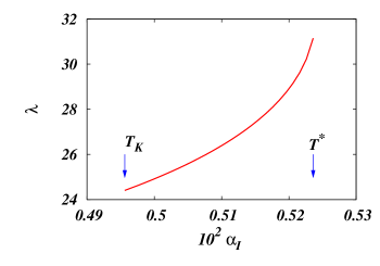
Figure 1: (Color online) The wandering length as a function of the inverse correlation length for $k_{0}=0.1$, $J=1/k_{0}^{2}$ and $v=0.001$.

III.2 Configurational entropy

Provided the existence of a transition to a non-ergodic regime has been established, we address the calculation of the number of metastable configurations, or configurational entropy. From (11) and (12) the configurational entropy can be obtained as

$$S_{c}=\beta\left.\frac{\partial F_{\psi}(m)}{\partial m}\right|_{m=1}.$$ (32)

Within the SCSA the replicated free energy is given by

$$2m\beta F_{\psi}=Tr\ln{{\cal G}^{-1}}+Tr\ln{{\cal D}^{-1}}-Tr(\Sigma{\cal G}).$$ (33)

Deriving with respect to $m$ and taking $m=1$ at the end, $S_{c}$ can be written as $S_{c}=s_{c}^{(1)}+s_{c}^{(2)}$ with:

$$s_{c}^{(1)}=-\frac{1}{2}\int\frac{d^{2}k}{(2\pi)^{2}}\left\{\ln{\left(1-\frac{{\cal F}(\vec{k})}{{\cal G}(\vec{k})}\right)}+\frac{{\cal F}(\vec{k})}{{\cal G}(\vec{k})}\right\}$$ (34)

and

$$s_{c}^{(2)} = \frac{1}{2}\int\frac{d^{2}k}{(2\pi)^{2}}\times$$ (35)

$$\times \left\{\ln{\left(1-\frac{v\Pi_{{\cal F}}(\vec{k})}{1+v\Pi_{{\cal G}}(\vec{k})}\right)}+\frac{v\Pi_{{\cal F}}(\vec{k})}{1+v\Pi_{{\cal G}}(\vec{k})}\right\}.$$

Performing the integrals we obtain

$$s_{c}^{(1)}=\frac{k_{0}\beta_{I}}{4}\left(1-\frac{\alpha_{I}}{\beta_{I}}\right)^{2}$$ (36)

and

$$s_{c}^{(2)} = \frac{1}{(16\pi J^{2}k_{0}^{4})^{2}}\frac{v^{2}k_{0}^{2}}{2\pi\alpha_{I}^{4}}\times$$ (37)

$$\times \left\{\left(1-\frac{\alpha_{I}}{\beta_{I}}\right)^{2}+\ln{\left[1-\left(1-\frac{\alpha_{I}}{\beta_{I}}\right)^{2}\right]}\right\}.$$

The first term is always positive but the second can be negative as the temperature decreases from the transition point. At some point the second negative term dominates over the first term and the configurational entropy becomes negative. As the entropy cannot be negative, this second characteristic temperature has been interpreted as signalling a transition to an ideal glass state. Below this temperature, called Kauzmann temperature ($T_{K}$) in the glass transition literature, the configurational entropy is zero and the system freezes into an amorphous state, which is, from this temperature down, a thermodynamically stable state. Then there is a temperature window, between $T_{K}$ and $T_{glass}$, in which the system has an exponentially large number of metastable states, as reflected in a finite value of $S_{c}$. In figure 2 we show the behavior of $S_{c}$ with the inverse correlation length $\alpha_{I}$. As in figure 1 the numerical values of the constants were fixed to $k_{0}=0.1$, $J=1/k_{0}^{2}$ and $v=0.001$.

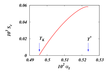
Figure 2: (Color online) Configurational entropy as a function of the inverse correlation length. The parameters were fixed to $k_{0}=0.1$, $J=1/k_{0}^{2}$ and $v=0.001$.

IV Discussion and conclusions

We have applied a replica approach for frustrated but non-disordered systems to a two dimensional stripe forming model with competing interactions. The model is representative of several well known systems, like high-Tc superconductors and ultrathin ferromagnetic films, which have been the subject of intense research. We have established the existence of a glass transition to a non-ergodic regime accompanied by an exponential number of long lived metastable states, responsible for slow dynamics and non-equilibrium effects. From a technical point of view, these results may come as no surprise since they are very similar to those already known in the three dimensional version of the model. Nevertheless, as stated in §I, the possible existence of glassy behavior in two dimensions is specially interesting due to the very different nature of the equilibrium phases of the systems in $d=2$ and $d=3$. From an equilibrium point of view, the existence of a continuous symmetry in $d=2$ associated with the isotropic nature of interactions implies that no long range order can survive. Instead of the stripe phase found in three dimensions, the relevant phase in two dimensions is a nematic oneBarci and Stariolo (2007, 2009) , with quasi-long-range orientational order and only short range translational order down to zero temperature. The nematic phase in a stripe forming system is characterized by a proliferation of topological defects which can naturally lead to an arrest of the dynamics as the temperature is lowered. In Refs. Barci and Stariolo, 2007, 2009 we showed that symmetry considerations allow the existence of other interaction terms in the Landau-Ginzburg expansion of the model defined in (1) and (2), leading to possible anisotropic phases of nematic character. The temperature at which the isotropic-nematic transition takes place was found to be proportional to the nematic order parameter couplings in the Landau expansion. These terms, although essential for the equilibrium behavior of the system, are not relevant for searching a possible freezing of the isotropic, high temperature correlations, as pursued in the present work. Thus, there are at least two characteristic temperatures determining, on one hand, the equilibrium isotropic/nematic phase transition and, on the other hand, a glassy non-equilibrium behavior of the system. A natural question now is to know the relation between both temperatures, which implies determining the dependence of the phenomenological nematic coupling constant on more microscopic parameters of the model, like $J$ and $k_{0}$. Some work in this direction has already been done Barci and Stariolo (2011) but the question is still not completely settled. Having a more microscopic model to begin with would allow to make quantitative predictions which could be in principle contrasted with experiments. Nevertheless the very existence and relevance of the nematic phase is still controversial and the existence of a glass-like transition adds a new ingredient to the theoretical understanding of low dimensional stripe forming systems.