Robust determination of the scalar boson couplings aaaTalk given by O. Éboli at the Rencontre de Moriond EW 2013.
We make a study of the indirect effects of new physics on the phenomenology of the “Higgs-like” particle. Assuming that the recently observed state is a light electroweak doublet scalar and the symmetry is realized linearly, we parametrize these effects in a model independent way in terms of an effective Lagrangian at the electroweak scale. We choose the dimension–six operator that allows us to better use all the available data to constrain the coefficients of the dimension-six operators. Subsequently we perform a global 6–parameter fit which allows for simultaneous determination of the standard model scalar couplings to electroweak gauge bosons, gluons, bottom quarks, and tau leptons. The results are based on the data released at Moriond 2013. Moreover, our formalism leads to strong constraints on the electroweak triple gauge boson couplings.
1 Low energy effective Lagrangian: the right of choice
The 2012 discovery of the state resembling the standard model scalar (SMS) marks the beginning of the direct study of electroweak symmetry breaking (EWSB) . To determine whether this new particle is the state predicted by the standard model (SM) we still must determine its properties like spin, parity, and couplings. Here we use a bottom–up approach to study the SMS couplings by parametrizing the deviations of the SM predictions by an effective Lagrangian.
We assume that the newly observed state is part of an electroweak scalar doublet and the gauge is linearly realized. The lowest order operators that modify the SMS couplings are of dimension–six . It is well known that there are 59 independent dimension–six operators up to flavor and Hermitian conjugation. However, there is a freedom in the choice of the basis of operators since operators connected by the equations of motion lead to the same –matrix elements . Thus, the determination of physical observables like branching ratios or production cross sections would be independent of the basis choice. Nevertheless independent does not mean equivalent. As a result of this reasoning, we propose that in the absence of theoretical prejudices it turns is beneficial to use a basis allowing for the use of largest dataset in our analyses. Therefore, a sensible (and certainly technically convenient) choice is to leave in the basis those operators which are directly related to the existing data, for example the bulk of precision electroweak measurements which have with the establishment of the SM.
In our analysis we characterize deviations from the predictions of the SM as
| (1) |
where are the dimension–six operators which involve gauge–bosons, and/or fermionic fields, and the SMS, with couplings and where is the characteristic scale. We assume operators to be and even and the conservation of baryon and lepton numbers. Our fit to the available datasets leads to constraints on that can be easily translated into SMS properties and into bounds on triple gauge boson couplings. The basic building blocks for the dimension–six operators are the SMS doublet and its covariant derivative, in our conventions, as well as, the hatted field strengths defined as and . The gauge couplings of () are denoted as () and the Pauli matrices by . The fermionic degrees of freedom are the lepton doublets , the quark doublets and the singlet fermions .
Here we directly present our choice of basis, however the detailed discussion of this choice can be found in this reference . In this basis the bosonic operators modifying the SMS interactions with the gauge bosons are
| (2) |
while the dimension–six operators relevant for the SMS interactions with fermions are
| (3) |
where we define , , and and where we denote the family indices by . In addition to the above operators the dimension–six basis also contains four–fermion interactions, dipole operators, as well as, the operator that leads to anomalous triple gauge couplings but does not modify the SMS interactions .
One important property of this choice of basis is the presence of the operators and that modify the SMS couplings to gauge boson pairs, as well as, the triple electroweak gauge couplings (TGC). This allows us to use the available TGC data to constrain the SMS properties. Moreover, the SMS data also have an impact on the present determination of the TGC as shown below .
Now we take advantage of and apply all available experimental information to the effect of reducing the number of relevant parameters in the analysis of the SMS data:
-
•
Considering that the couplings to fermions are in agreement with the SM at the level of per mil , the operators modifying these couplings will have coefficients so constrained that they will have no impact in the SMS physics with the present statistics. Consequently, we remove the operators from our analyses.
-
•
The precision electroweak parameters and strongly constrain the coefficients of and , therefore, we also neglect their contributions.
-
•
The off–diagonal part of is strongly constrained by data on low–energy flavor–changing interactions. Consequently we also discard them from our basis.
-
•
Flavor diagonal from the first and second generations only have an effect on the present Higgs data via their contribution to the SMS–gluon–gluon and SMS–– vertex at the one loop level. The form factors are very suppressed for light fermion loops and correspondingly their effect is totally negligible in the analysis. Therefore, we keep the fermionic operators , and only.
-
•
Tree level information concerning production has very large errors still. So the parameter effectively contributes only to the one–loop SMS couplings gluon and photon pairs. Presently these contributions can be absorbed into the redefinition of the parameters and , therefore, we take . In the future, when a larger luminosity is accumulated, it will be necessary to reintroduce as one of the parameters in the fit.
Therefore, at the end of the day, the effective Lagrangian relevant to our analyses is
| (4) |
that contains 6 unknown parameters .
To obtain the present constraints on the six unknown parameters we construct a chi-square function using all available data on the SMS production and decay coming from LHC and Tevatron and also on TGC and electroweak precision data (EWPD). The details of the statistical analyses are presented in reference .
2 Results
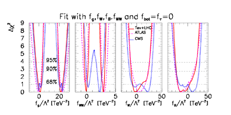
In order to compare the bounds on the SMS couplings coming from ATLAS and CMS data we considered a scenario where the SMS couplings to fermions take on their SM values, i.e., we set and we fit the available data with as the relevant free independent parameters. Figure 1 depicts the as a function of each of the four free parameters after having marginalized over the three unshown parameters. As we can see in the left panel, as a function of possesses two degenerate minima caused by interference between SM and the anomalous contributions. For the case of the chi–square dependence on again there is an interference between SM and anomalous contributions, however, the degeneracy of the minima is lifted as a result of the coupling contributing to SMS decays into photons, and , as well as in associated and vector boson fusion production mechanisms. Moreover, we can see from this figure that the CMS, ATLAS and combined data exhibit a similar chi–square behavior with respect to the fitting parameters and that the ATLAS and CMS data lead to similar bounds on the SMS couplings at 90% CL.
The effect of combining the SMS data with the TGC data and EWPD is presented in Fig. 2 where a different set of free parameters was used for each row. In the upper row of the figure the SMS couplings to fermions are the SM ones while in the lower row the set of fitting parameters is augmented with the inclusion of anomalous bottom and tau couplings, and , i.e. we perform a six–parameter fit in . When including EWPD a scale of 10 TeV was assumed in the evaluation of logarithms appearing in the expressions for , and ; see reference for further details. Comparing the panels in the same column we can see that the impact of the different datasets is similar in the two scenarios depicted in this figure. Because and are the only fit parameters modifying the TGC at tree level, they show the largest impact of the TGC data, particularlly . Moreover, the inclusion of the EWPD in the fit has the affect of reducing the errors on and significantly, in addition to lifting the near degeneracy on .
Let us explore in more detail the two scenarios presented in Figure 2, focusing on the effects of allowing for the modification of Higgs couplings to fermions. Comparing the panels in the upper row with the ones in the lower row we can see the allowed range of becomes much greater for the latter case, where the range for is large as well. This behavior has origins in the fact that large causes the SMS branching ratio into pairs of b–quark to approach 1, so in order to fit the data for any channel with a final state F with , the gluon fusion cross section is enhanced in order to make up for the dilution of branching ratios. This occurs due to a strong correlation between allowed values of . This is illustrated in Fig. 3 which depicts the strong correlation between the allowed values of .
Still from Fig. 2 we can see that allowing for and has a small impact on the parameters affecting the SMS couplings to the electroweak gauge bosons and as shown by comparing the corresponding upper and lower panels. Concerning , it does not possess any strong correlation with other variables because the data on cuts off all strong correlations between and . At the end, the introduction of has a little impact on the determination of the other free parameters.
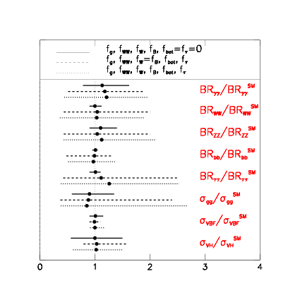
We present in Fig. 4 the chi-square dependence on branching ratios and production cross sections for the two scenarios presented in Fig. 2. The effect of and on physical observables can be seen by comparing the upper and lower rows of this figure: We can easily see that bounds on branching ratios and cross sections get loosened, with the VBF and VH production cross sections being the least affected quantities while the gluon fusion cross section is the one which becomes less constrained. The reason for this reduction of the constraints is the strong correlation between and just mentioned. We summarize the bounds on SMS production cross sections and branching ratios in the left panel of Fig. 5 that shows that the SM predictions for the SMS properties are in good agreement with the available data.
The operators and modify not only the SMS interactions, but also give rise to TGC as we have already commented:
| (5) |
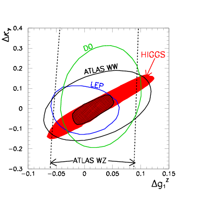
where stands for the sine (cosine) of the weak mixing angle. Therefore, we use our framework to get bounds on TGC and we present them in the right panel of Fig. 5, where we can see that the present SMS physics bounds on show a non-negligible correlation. This stems from the correlation imposed on the high values of and from their tree level contribution to data, a correlation which is transported to the plane. Furthermore, the right panel of this figure also shows that the present bounds on from the analysis of SMS data are stronger than those coming from direct TGC studies at the LHC.
The most important lesson that we can learn from the right panel of Fig. 5 is the complementarity of the bounds on new physics effects originating from the analysis of SMS signals and from studies of the electroweak gauge–boson couplings . To assess the potential of this complementarity we combine the present bounds derived from SMS data with those from the TGC analysis from LEP, Tevatron and LHC shown in Fig. 5. Clearly the inclusion of the SMS data leads to stronger constraints on TGC. The combined 1 1dof allowed ranges are
3 Discussion and conclusions
Here, we applied a bottom–up approach to describe possible departures of the SMS couplings from the SM predictions. Working in a model independent framework the effects of the departures can be parametrized in terms of an effective Lagrangian, more specifically we chose a basis of the dimension–six operators such that we could use the largest possible dataset to constrain the SMS couplings. In this general framework the modifications of the couplings of the SMS field to electroweak gauge bosons are related to the anomalous triple gauge–boson vertex . Our fit to the presently available data show that the SMS branching ratios and cross sections are compatible with the SM at 1 level. Moreover, the analysis of the Higgs boson production data at LHC and Tevatron is able to furnish bounds on the related TGC which, in some cases, are tighter than those obtained from direct triple gauge–boson coupling analysis. In the near future the LHC collaborations will release their analysis of TGC with the larger statistics of the 8 TeV run. The combination of those with the present results from SMS data has the potential to furnish the strongest constraints on new physics effects on the EWSB sector until further luminosity can be accumulated bbb As new data become available we will present the latest results in the site http://hep.if.usp.br/Higgs.
Acknowledgments
This work is supported by Conselho Nacional de Desenvolvimento Científico e Tecnológico (CNPq), by Fundação de Amparo à Pesquisa do Estado de São Paulo (FAPESP), by USA-NSF grant PHY-09-6739, by CUR Generalitat de Catalunya grant 2009SGR502, by MICINN FPA2010-20807 and consolider-ingenio 2010 program CSD-2008-0037, by EU grant FP7 ITN INVISIBLES (Marie Curie Actions PITN-GA-2011-289442), and by ME FPU grant AP2009-2546.
References
References
- [1] S. Chatrchyan et al. [CMS Collaboration], Phys. Lett. B 716 (2012) 30. G. Aad et al. [ATLAS Collaboration], Phys. Lett. B 716 (2012) 1.
- [2] W. Buchmuller and D. Wyler, Nucl.Phys. B268, 621 (1986); C. N. Leung, S. Love, and S. Rao, Z.Phys. C31, 433 (1986); A. De Rujula, M. Gavela, P. Hernandez, and E. Masso, Nucl.Phys. B384, 3 (1992); M. Gonzalez-Garcia, Int.J.Mod.Phys. A14, 3121 (1999); K. Hagiwara, R. Szalapski, and D. Zeppenfeld, Phys.Lett. B318, 155 (1993).
- [3] B. Grzadkowski, M. Iskrzynski, M. Misiak and J. Rosiek, JHEP 1010, 085 (2010).
- [4] H. D. Politzer, Nucl. Phys. B 172, 349 (1980); H. Georgi, Nucl. Phys. B 361, 339 (1991); C. Arzt, Phys. Lett. B 342, 189 (1995); H. Simma, Z. Phys. C 61, 67 (1994).
- [5] T. Corbett, O. J. P. Eboli, J. Gonzalez-Fraile and M. C. Gonzalez-Garcia, Phys. Rev. D 86, 075013 (2012); T. Corbett, O. J. P. Eboli, J. Gonzalez-Fraile and M. C. Gonzalez-Garcia, Phys. Rev. D 87, 015022 (2013); T. Corbett, O. J. P. Eboli, J. Gonzalez-Fraile and M. C. Gonzalez-Garcia, arXiv:1304.1151 [hep-ph].
- [6] F. de Campos, M. C. Gonzalez-Garcia and S. F. Novaes, Phys. Rev. Lett. 79, 5210 (1997) [hep-ph/9707511]; M. C. Gonzalez-Garcia, S. M. Lietti and S. F. Novaes, Phys. Rev. D 57, 7045 (1998) [hep-ph/9711446]; O. J. P. Eboli, M. C. Gonzalez-Garcia, S. M. Lietti and S. F. Novaes, Phys. Lett. B 434, 340 (1998) [hep-ph/9802408]; M. C. Gonzalez-Garcia, S. M. Lietti and S. F. Novaes, Phys. Rev. D 59, 075008 (1999) [hep-ph/9811373]; O. J. P. Eboli, M. C. Gonzalez-Garcia, S. M .Lietti and S. F. Novaes, Phys. Lett. B 478, 199 (2000) [hep-ph/0001030].
- [7] [ALEPH and CDF and D0 and DELPHI and L3 and OPAL and SLD and LEP Electroweak Working Group and Tevatron Electroweak Working Group and SLD Electroweak and Heavy Flavour Groups Collaborations], arXiv:1012.2367 [hep-ex].
- [8] ATLAS Collaboration, ATLAS-CONF-2012-160; ATLAS Collaboration, ATLAS-CONF-2012-161; ATLAS Collaboration, ATLAS-CONF-2013-013; ATLAS Collaboration, ATLAS-CONF-2013-030; ATLAS Collaboration, ATLAS-CONF-2013-009; CMS Collaboration, CMS PAS HIG-13-004; CMS Collaboration, CMS PAS HIG-12-044; CMS Collaboration, CMS PAS HIG-13-002; CMS Collaboration, CMS PAS HIG-13-003; CMS Collaboration, CMS PAS HIG-13-006; ATLAS Collaboration, ATLAS-CONF-2012-091; ATLAS Collaboration, ATLAS-CONF-2013-012; CMS Collaboration, CMS PAS HIG-13-001; The CDF Collaboration, the D0 Collaboration, Higgs Working Group, t. T. N. Physics, (2012), arXiv:1207.0449.
- [9] The LEP collaborations and The LEP TGC Working group LEPEWWG/TGC/2003-01; V. M. Abazov et al. [D0 Collaboration], Phys. Lett. B 718, 451 (2012); T. Aaltonen et al. [CDF Collaboration], Phys. Rev. D 86, 031104 (2012); T. Aaltonen et al. [CDF Collaboration], Phys. Rev. Lett. 104, 201801 (2010); G. Aad et al. [ATLAS Collaboration], arXiv:1210.2979 [hep-ex]; G. Aad et al. [ATLAS Collaboration], Eur. Phys. J. C 72, 2173 (2012); G. Aad et al. [ The ATLAS Collaboration], arXiv:1302.1283 [hep-ex]; CMS Collaboration, https://twiki.cern.ch/twiki/bin/view/CMSPublic/PhysicsResultsSMP12005; CMS Collaboration, https://twiki.cern.ch/twiki/bin/view/CMSPublic/PhysicsResultsEWK11009; S. Chatrchyan et al. [CMS Collaboration], Eur. Phys. J. C 73, 2283 (2013).