Angle-dependent Gap state in Asymmetric Nuclear Matter

Abstract

We propose an axi-symmetric angle-dependent gap (ADG) state with the broken rotational symmetry in isospin-asymmetric nuclear matter. In this state, the deformed Fermi spheres of neutron and proton increase the pairing probabilities along the axis of symmetry breaking near the average Fermi surface. We find the state possesses lower free energy and larger gap value than the angle-averaged gap state at large isospin asymmetries. These properties are mainly caused by the coupling of different $m_{j}$ components of the pairing gap. Furthermore, we find the transition from the ADG state to normal state is of second order and the ADG state vanishes at the critical isospin asymmetry $\alpha_{c}$ where the angle-averaged gap vanishes.

I Introduction

The neutron-proton (n-p) pairing properties play an important role in the description of superfluidity of finite nuclei with $N\simeq Z$ Fn ; Fn2 and symmetric nuclear matterSnm1 ; Snm2 ; Snm3 . In general, the n-p pair correlations are considered in different dominant partial-wave channels, depending on the relevant density and temperature. For weakly isospin-asymmetric systems, the isospin singlet attractive ${}^{3}S_{1}-^{3}D_{1}$ (${}^{3}SD_{1}$) channel dominates the pairing interaction at relatively low densities around the nuclear saturation density due to the tensor component of the nuclear forceSnm1 ; Sdd ; Sdd2 ; Sdd3 ; Sdd4 ; Sdd5 , and the ${}^{3}D_{{}_{2}}$ channel dominates at high densities well above the saturation densityD1 ; D2 . In neutron star matter, the n-p pair correlations are strongly suppressed by the isospin-asymmetry. However, the dilute nuclear matter at sub-saturation densities in supernovas and hot proto-neutron stars can support ${}^{3}SD_{1}$ channel pairingSdd3 ; Sh1 ; Sh2 ; Sh3 .

Since n-p pair correlations depend crucially on the overlap between the neutron and proton Fermi surfaces, the pairing gap is suppressed rapidly as the system is driven out of the isospin-symmetric state. At zero temperature, a small isospin-asymmetry is enough to prevent the formation of the Cooper pairs between neutrons and protons with momenta $\overrightarrow{k}$ and $-\overrightarrow{k}$ around their average Fermi surface where the contribution to superfluidity is dominant. Near zero temperature, thermal excitations can reduce the suppression by smearing out the two Fermi surfaces, however, it is ineffective when the separation between the two Fermi surfaces is large compared to the temperature. In isospin-asymmetric nuclear matter, the FFLO ff ; lo state and the DFS (deformed Fermi surfaces) dfs state have been studied in Refs.ffn ; dfsn . In a FFLO state, the shift of the two Fermi spheres with respect to each other, resulting form the collective motion of the Cooper pairs with a finite momentum, enhances the overlap between the neutron and proton Fermi surfaces. The overlap regions then provide the kinematical phase space for n-p pairing phenomena to occur. And in a DFS state, the deformation of the neutron and proton Fermi surfaces may increase the phase-space overlap between the two Fermi surfaces. Both in these two kinds of possible superfluid states, the quasiparticle excitation spectra are no longer isotropic, since the anisotropic overlapping configurations could increase the pairing energy. On the other hand, the usually adopted angle-averaging procedure in the previous calculationsSdd2 ; ffn , which has been proved to be a quite good approximation in symmetry nuclear matter aap , considers the gap as an isotopic gap by ignoring the angle dependence. As the true ground state corresponds to the anisotropic overlapping configuration, the angle-averaging procedure may be an insufficient approximation in isospin-asymmetric nuclear matter.

In this paper we consider an axi-symmetric angle dependent gap (ADG) state, and give a general and systematic comparison between the ADG state and the angle-averaged gap (AAG) state in isospin-asymmetric nuclear matter. The paper is organized as follows: In Sec. II we briefly review the formalism for the isotropic AAG state, and derive the angle dependent gap equations from the Gorkov equations. The numerical solutions of these equations are shown and discussed in Sec. III, where we compare the AAG state with the ADG state at finite temperature. Finally, a summary and a conclusion are given in Sec. IV.

II Formalism

For isospin-asymmetric nuclear matter, the isospin singlet ${}^{3}SD_{1}$ pairing channel dominates the attractive pairing force at low densities. In this case we can consider ${}^{3}SD_{1}$ channel only, the gap function is thus expanded according to

$$\Delta_{\sigma_{1},\sigma_{2}}(\textbf{k})=\sum_{l,m_{j}}\Delta_{l}^{m_{j}}(k)[G_{l}^{m_{j}}(\textbf{\^{k}})]_{\sigma_{1},\sigma_{2}},$$ (1)

with the elements of the spin-angle matrices

$$[G_{l}^{m_{j}}(\textbf{\^{k}})]_{\sigma_{1},\sigma_{2}}\equiv\langle\frac{1}{2}\sigma_{1},\frac{1}{2}\sigma_{2}\mid 1\sigma_{1}+\sigma_{2}\rangle\langle 1\sigma_{1}+\sigma_{2},lm_{l}\mid 1m_{j}\rangle Y_{l}^{m_{l}}(\textbf{\^{k}}),$$

where $m_{j}$ and $m_{l}$ are the projections of the total angular momentum $j=1$ and the orbit angular momentum $l=0,2$ of the pair, respectively. The $Y_{l}^{m_{l}}(\textbf{\^{k}})$ denotes the spherical harmonic with $\textbf{\^{k}}\equiv\textbf{k}/k$. The anomalous density matrix follows the same expansion. Moreover the time-reversal invariance implies that

$$\Delta_{\sigma_{1},\sigma_{2}}(\textbf{k})=(-1)^{1+\sigma_{1}+\sigma_{2}}\Delta_{-\sigma_{1},-\sigma_{2}}^{*}(\textbf{k}).$$ (3)

Namely, the pairing gap matrix $\Delta(\textbf{k})$ in spin space possesses the property

$$\Delta(\textbf{k})\Delta^{{\dagger}}(\textbf{k})=ID^{2}(\textbf{k}),$$ (4)

i.e., the gap function has the structure of a ``unitary triplet" state aap . $I$ is the identity matrix and $D(\textbf{k})$ is a scalar quantity in spin space.

Once the the isospin singlet ${}^{3}SD_{1}$ channel has been selected, the pairing gap is an isoscalar and the isospin indices can be dropped off. The proton/neutron propagators follow from the solution of the Gorkov equations, and can be present in the form ($\hbar=1$)

$$\textbf{G}_{\sigma,\sigma^{{}^{\prime}}}^{(p/n)}(\textbf{k},\omega_{m})=-\delta_{\sigma,\sigma^{{}^{\prime}}}\frac{i\omega_{m}+\xi_{\textbf{k}}\mp\delta\varepsilon_{\textbf{k}}}{(i\omega_{m}+E_{\textbf{k}}^{+})(i\omega_{m}-E_{\textbf{k}}^{-})}.$$ (5)

The neutron-proton anomalous propagator matrix in spin space has the form

$$\textbf{F}^{{\dagger}}(\textbf{k},\omega_{m})=-\frac{\Delta^{{\dagger}}(\textbf{k})}{(i\omega_{m}+E_{\textbf{k}}^{+})(i\omega_{m}-E_{\textbf{k}}^{-})},$$ (6)

where $\omega_{m}$ are the Matsubara frequencies, the uper sign in $\textbf{G}_{\sigma,\sigma^{{}^{\prime}}}^{(p/n)}$ corresponds to protons, and the lower to neutrons. The quasiparticle excitation spectra are determined by finding the poles of the propagators in Gorkov equations,

$$E_{\textbf{k}}^{\pm}=\sqrt{\xi_{\textbf{k}}^{2}+\frac{1}{2}Tr(\Delta\Delta^{{\dagger}})\pm\frac{1}{2}\sqrt{[Tr(\Delta\Delta^{{\dagger}})]^{2}-4\det(\Delta\Delta^{{\dagger}})}}\pm\delta\varepsilon_{\textbf{k}},$$ (7)

where

$$\xi_{\textbf{k}}\equiv\frac{1}{2}(\varepsilon_{\textbf{k}}^{p}+\varepsilon_{\textbf{k}}^{n}),\delta\varepsilon_{\textbf{k}}\equiv\frac{1}{2}(\varepsilon_{\textbf{k}}^{p}-\varepsilon_{\textbf{k}}^{n}),$$

and $\varepsilon_{\textbf{k}}^{(n,p)}$ are the single particle energies of neutrons and protons. Using the ``unitary" property in Eq. (4), the quasiparticle spectra are simplified to

$$E_{\textbf{k}}^{\pm}=\sqrt{\xi_{\textbf{k}}^{2}+D^{2}(\textbf{k})}\pm\delta\varepsilon_{\textbf{k}},$$ (8)

which are separated into two branches due to the isospin-asymmetry.

In the present ``unitary triplet" case, the gap equation at finite temperature can be written in the standard form

$$\Delta_{\sigma_{1},\sigma_{2}}(\textbf{k})=-\sum_{\textbf{k}^{{}^{\prime}}}\sum_{\sigma_{1}^{{}^{\prime}},\sigma_{2}^{{}^{\prime}}}<\textbf{k}\sigma_{1},-\textbf{k}\sigma_{2}\mid V\mid\textbf{k}^{{}^{\prime}}\sigma_{1}^{{}^{\prime}},-\textbf{k}^{{}^{\prime}}\sigma_{2}^{{}^{\prime}}>$$

$$\times\frac{\Delta_{\sigma_{1}^{{}^{\prime}},\sigma_{2}^{{}^{\prime}}}(\textbf{k}^{{}^{\prime}})}{2\sqrt{\xi_{\textbf{k}^{{}^{\prime}}}^{2}+D^{2}(\textbf{k}^{{}^{\prime}})}}[1-f(E_{\textbf{k}^{{}^{\prime}}}^{+})-f(E_{\textbf{k}^{{}^{\prime}}}^{-})],$$ (9)

where $f(E)=[1+\exp(\beta E)]^{-1}$ is the Fermi distribution at finite temperature and $V$ is the interaction in the ${}^{3}SD_{1}$ channel. $\beta^{-1}=k_{B}T$, where $k_{B}$ is the Boltzmann constant and $T$ is the temperature. Substituting the expansion Eq.(1) into Eqs.(9) and (4), one gets a set of coupled equations for the quantities $\Delta_{l}^{m_{j}}(k)$

$$\Delta_{l}^{m_{j}}(k)=\frac{-1}{\pi}\int_{0}^{\infty}dk^{{}^{\prime}}k^{{}^{\prime}2}\sum_{l^{{}^{\prime}}=0,2}i^{l^{{}^{\prime}}-l}V^{l^{{}^{\prime}}l}_{\lambda}(k^{{}^{\prime}},k)\sum_{l^{{}^{\prime\prime}}\mu}\Delta_{l^{{}^{\prime\prime}}}^{\mu}(k^{{}^{\prime}})$$

$$\times\int d\Omega_{\textbf{k}^{{}^{\prime}}}Tr[G_{l^{{}^{\prime}}}^{m_{j}*}(\textbf{\^{k}}^{{}^{\prime}})G_{l^{{}^{\prime\prime}}}^{\mu}(\textbf{\^{k}}^{{}^{\prime}})]\frac{1-f(E_{\textbf{k}^{{}^{\prime}}}^{+})-f(E_{\textbf{k}^{{}^{\prime}}}^{-})}{\sqrt{\xi_{\textbf{k}^{{}^{\prime}}}^{2}+D^{2}(\textbf{k}^{{}^{\prime}})}},$$ (10)

with

$$D^{2}(\textbf{k})=\frac{1}{2}Tr(\Delta\Delta^{{\dagger}})=\sum_{ll^{{}^{\prime}}=0,2}\sum_{m_{j}m_{j^{{}^{\prime}}}}\Delta_{l}^{m_{j}*}(k)\Delta_{l^{{}^{\prime}}}^{m_{j^{{}^{\prime}}}}(k)Tr[G_{l}^{m_{j}{\dagger}}(\textbf{\^{k}})G_{l^{{}^{\prime}}}^{m_{j^{{}^{\prime}}}}(\textbf{\^{k}})],$$

where

$$V^{l^{{}^{\prime}}l}_{\lambda}(k^{{}^{\prime}},k)\equiv<k^{{}^{\prime}}\mid V^{l^{{}^{\prime}}l}_{\lambda}\mid k>=\int_{0}^{\infty}r^{2}drj_{l^{{}^{\prime}}}(k^{{}^{\prime}}r)V^{l^{{}^{\prime}}l}_{\lambda}(r)j_{l}(kr),$$ (12)

is the matrix elements of the NN interaction in different partial wave ($\lambda=T,S,l,l^{{}^{\prime}}$) channels. Here $\lambda$ corresponds to the coupled ${}^{3}SD_{1}$ channel. Following from Eq.(5), we can get the densities of neutrons and protons

$$\rho^{(p/n)}=\sum_{\textbf{k},\sigma}n_{\sigma}^{(p/n)}(\textbf{k}),$$ (13)

with the distributions

$$n_{\sigma}^{(p/n)}(\textbf{k})=\{\frac{1}{2}(1+\frac{\xi_{\textbf{k}}}{\sqrt{\xi_{\textbf{k}}^{2}+D^{2}(\textbf{k})}})f(E_{\textbf{k}}^{\pm})$$

$$+\frac{1}{2}(1-\frac{\xi_{\textbf{k}}}{\sqrt{\xi_{\textbf{k}}^{2}+D^{2}(\textbf{k})}})[1-f(E_{\textbf{k}}^{\mp})]\}.$$ (14)

Summation over frequencies in Eq.(6) leads to the density matrix of the particles in the condensate,

$$\nu(\textbf{k})=\frac{\Delta(\textbf{k})}{2\sqrt{\xi_{\textbf{k}}^{2}+D^{2}(\textbf{k})}}[1-f(E_{\textbf{k}}^{+})-f(E_{\textbf{k}}^{-})].$$ (15)

It is essential that the coupled Eqs.(10) and (13) should be solved self-consistently.

The six components $\Delta_{l}^{m_{j}}(k)$ of $\Delta(\textbf{k})$ are strongly coupled due to the angle dependent energy denominator $\sqrt{\xi_{\textbf{k}}^{2}+D^{2}(\textbf{k})}$ in Eqs.(10) and (13). The equations are thus complicated to be solved accurately, and approximation has been employed. Before introducing the angle-averaging procedure and ADG, we need to substitute $\Delta_{l}^{m_{j}}(k)$ with real variables. From Eq.(3) we can find the relation

$$\Delta_{l}^{m_{j}*}(k)=-(-1)^{m_{j}}\Delta_{l}^{-m_{j}}(k).$$ (16)

Therefore, we have four independent components $\Delta_{0}^{0}(k)$, $\Delta_{0}^{1}(k)$, $\Delta_{2}^{0}(k)$ and $\Delta_{2}^{1}(k)$ for ${}^{3}SD_{1}$ channel , and we can describe $\Delta_{l}^{m_{j}}(k)$ as

$$\Delta_{0}^{0}(k) =i\delta_{0}(k),$$

$$\Delta_{0}^{1}(k) =\delta_{1}(k)+in_{1}(k),$$

$$\Delta_{2}^{0}(k) =i\delta_{2}(k),$$

$$\Delta_{2}^{1}(k) =\delta_{3}(k)+in_{3}(k),$$ (17)

where the six independent variables $\delta_{0}(k)$, $\delta_{1}(k)$, $n_{1}(k)$, $\delta_{2}(k)$, $\delta_{3}(k)$ and $n_{3}(k)$ are real quantities. Inserting Eq.(17) into Eq.(11), we get

$$D^{2}(\textbf{k})= \frac{1}{32\pi}\Big{\{}4\delta_{0}^{2}(k)-4\sqrt{2}\delta_{0}(k)\delta_{2}(k)[3\cos^{2}\theta-1]+2\delta_{2}^{2}(k)[3\cos^{2}\theta-1]$$

$$+8[\delta_{1}^{2}(k)+n_{1}^{2}(k)]+8[\delta_{3}^{2}(k)+n_{3}^{2}(k)]+6[\delta_{3}^{2}(k)+n_{3}^{2}(k)]\sin^{2}\theta$$

$$+4\sqrt{2}n_{1}(k)n_{3}(k)[3\cos^{2}\theta-1]+4\sqrt{2}\delta_{1}(k)\delta_{3}(k)[3\cos^{2}\theta-1]$$

$$+12[2\delta_{0}(k)n_{3}(k)+2\delta_{2}(k)n_{1}(k)-\sqrt{2}\delta_{2}(k)n_{3}(k)]\cos\theta\sin\theta\cos\varphi$$

$$+12[2\delta_{1}(k)\delta_{2}(k)+2\delta_{0}(k)\delta_{3}(k)-\sqrt{2}\delta_{2}(k)\delta_{3}(k)]\cos\theta\sin\theta\sin\varphi$$

$$+6[n_{3}^{2}(k)-\delta_{3}^{2}(k)+2\sqrt{2}\delta_{1}(k)\delta_{3}(k)-2\sqrt{2}n_{1}(k)n_{3}(k)]\sin^{2}\theta\cos 2\varphi$$

$$+12[\delta_{3}(k)n_{3}(k)-\sqrt{2}\delta_{1}(k)n_{3}(k)-\sqrt{2}\delta_{3}(k)n_{1}(k)]\sin^{2}\theta\sin 2\varphi\Big{\}}.$$

II.1 The angle-averaging procedure

Supposing the angle dependence of the energy denominator $\sqrt{\xi_{\textbf{k}}^{2}+D^{2}(\textbf{k})}$ can be neglected, the gap equations are simplified by substituting $D^{2}(\textbf{k})$ with its angular average value,

$$D^{2}(\textbf{k})\rightarrow d^{2}(k)=\frac{1}{4\pi}\int d\Omega_{\textbf{k}}D^{2}(\textbf{k})$$ (19)

$$=\frac{1}{8\pi}\Big{[}2\delta_{1}^{2}(k)+\delta_{0}^{2}(k)+2n_{1}^{2}(k)+2\delta_{3}^{2}(k)+\delta_{2}^{2}(k)+2n_{3}^{2}(k)\Big{]}.$$

Thereby, the energy denominator and the quasiparticle spectra are isotropic. Noting the properties of $G_{l}^{m_{j}}(\textbf{\^{k}})$

$$\int d\Omega_{\textbf{k}}Tr[G_{l}^{m_{j}*}(\textbf{\^{k}})G_{l^{{}^{\prime}}}^{m_{j^{{}^{\prime}}}*}(\textbf{\^{k}})]=\delta_{ll^{{}^{\prime}}}\delta_{m_{j}m_{j^{{}^{\prime}}}},$$ (20)

the different $m_{j}$ components $\Delta_{l}^{m_{j}}(k)$ with the same $l$ become uncoupled and all equal to each other. It follows that

$$\delta_{1}(k)=n_{1}(k)=\sqrt{\frac{1}{2}}\delta_{0}(k),\delta_{3}(k)=n_{3}(k)=\sqrt{\frac{1}{2}}\delta_{2}(k),$$ (21)

and

$$d^{2}(k)=\frac{3}{8\pi}[\delta_{0}^{2}(k)+\delta_{2}^{2}(k)].$$ (22)

Taking the normalization

$$\Delta_{0}(k)=\sqrt{\frac{3}{8\pi}}\delta_{0}(k),\Delta_{2}(k)=-\sqrt{\frac{3}{8\pi}}\delta_{2}(k),$$ (23)

the set of equations in Eq.(10) reduces to two coupled equations for the ${}^{3}S_{1}$ and ${}^{3}D_{1}$ gap components $\Delta_{0}(k)$ and $\Delta_{2}(k)$, respectively. They read

$$\left(\begin{array}[]{l}\Delta_{0}\\ \Delta_{2}\end{array}\right)(k)=\frac{-1}{\pi}\int dk^{{}^{\prime}}k^{{}^{\prime}2}\left(\begin{array}[]{ll}V^{00}&V^{02}\\ V^{20}&V^{22}\end{array}\right)(k,k^{{}^{\prime}})\frac{1-f(E_{k^{{}^{\prime}}}^{+})-f(E_{k^{{}^{\prime}}}^{-})}{\sqrt{\xi_{\textbf{k}^{{}^{\prime}}}^{2}+D^{2}(k^{{}^{\prime}})}}\left(\begin{array}[]{l}\Delta_{0}\\ \Delta_{2}\end{array}\right)(k^{{}^{\prime}})$$ (30)

, (31)

where $V^{00}$, $V^{02}$, $V^{20}$, $V^{22}$ are given in Eq.(12) with $l,l^{{}^{\prime}}=0,2$ and

$$E^{\pm}_{k}=\sqrt{\xi_{\textbf{k}}^{2}+D^{2}(k)}\pm\delta\varepsilon_{\textbf{k}}, D^{2}(k)\equiv d^{2}(k)=\Delta_{0}^{2}(k)+\Delta_{2}^{2}(k).$$ (32)

Eqs.(13), (24) and (25) compose the angle-averaged gap equations and should be solved simultaneously for isospin-asymmetric nuclear matter. The quasiparticle spectra here are isotropic and the gapless excitation exists at large asymmetry ($|\delta\varepsilon_{\textbf{k}_{F}}|\geq D(k_{F})$) near zero temperature.

II.2 The angle dependent gap

As pointed out in the Sec.I, the angle dependence of quasiparticle spectra due to $D^{2}(\textbf{k})$ may increase the phase-space overlap of neutron and proton near their average Fermi surface. We consider an axi-symmetric $D^{2}(\textbf{k})$ solution which corresponds to an axi-symmetric deformation of the neutron and proton Fermi spheres. From the expression in Eq.(18), the axi-symmetric solutions are restricted by

$$2\delta_{0}(k)n_{3}(k)+2\delta_{2}(k)n_{1}(k)-\sqrt{2}\delta_{2}(k)n_{3}(k)=0,$$

$$2\delta_{1}(k)\delta_{2}(k)+2\delta_{0}(k)\delta_{3}(k)-\sqrt{2}\delta_{2}(k)\delta_{3}(k)=0,$$

$$n_{3}^{2}(k)-\delta_{3}^{2}(k)+2\sqrt{2}\delta_{1}(k)\delta_{3}(k)-2\sqrt{2}n_{1}(k)n_{3}(k)=0,$$

$$\delta_{3}(k)n_{3}(k)-\sqrt{2}\delta_{1}(k)n_{3}(k)-\sqrt{2}\delta_{3}(k)n_{1}(k)=0.$$ (33)

There exists only one nontrivial solution

$$\delta_{1}(k)=n_{1}(k)=\delta_{3}(k)=n_{3}(k)=0,$$ (34)

which corresponds to the $m_{j}=0$ gap components of $\Delta_{l}^{m_{j}}(k)$. In this case

$$D^{2}(\textbf{k})\rightarrow D^{2}(k,\theta)= \frac{1}{8\pi}\Big{[}\delta_{0}^{2}(k)-\sqrt{2}\delta_{0}(k)\delta_{2}(k)(3\cos^{2}\theta-1)$$ (35)

$$+\delta_{2}^{2}(k)\frac{3\cos^{2}\theta+1}{2}\Big{]}.$$

Using the normalization

$$\Delta_{0}(k)=\sqrt{\frac{1}{8\pi}}\delta_{0}(k),\Delta_{2}(k)=-\sqrt{\frac{1}{8\pi}}\delta_{2}(k),$$ (36)

one gets the angle dependent gap equations

$$\left(\begin{array}[]{l}\Delta_{0}\\ \Delta_{2}\end{array}\right)(k) =\frac{-1}{\pi}\int dk^{{}^{\prime}}k^{{}^{\prime}2}\left(\begin{array}[]{ll}V^{00}&V^{02}\\ V^{20}&V^{22}\end{array}\right)(k,k^{{}^{\prime}})$$ (46)

$$\times\int d\Omega_{\textbf{k}^{{}^{\prime}}}\frac{1-f(E_{k^{{}^{\prime}}}^{+})-f(E_{k^{{}^{\prime}}}^{-})}{\sqrt{\xi_{\textbf{k}^{{}^{\prime}}}^{2}+D^{2}(k^{{}^{\prime}},\theta)}}\left(\begin{array}[]{ll}\emph{f}(\theta)&\emph{g}(\theta)\\ \emph{g}(\theta)&\emph{h}(\theta)\end{array}\right)\left(\begin{array}[]{l}\Delta_{0}\\ \Delta_{2}\end{array}\right)(k^{{}^{\prime}}),$$

with the following axi-symmetric quantities,

$$D^{2}(k,\theta) =\Delta_{0}^{2}(k)+\sqrt{2}\Delta_{0}(k)\Delta_{2}(k)[3\cos^{2}\theta-1]+\Delta_{2}^{2}(k)[\frac{3\cos^{2}\theta+1}{2}],$$

$$E^{\pm}_{k} =\sqrt{\xi_{\textbf{k}}^{2}+D^{2}(k,\theta)}\pm\delta\varepsilon_{\textbf{k}}.$$ (47)

The angle matrix $\left(\begin{array}[]{ll}\emph{f}(\theta)&\emph{g}(\theta)\\ \emph{g}(\theta)&\emph{h}(\theta)\end{array}\right)$ comes from the coupling among the different $m_{j}$ components of $\Delta(\textbf{k})$. The matrix elements are

$$\emph{f}(\theta) =Tr[G_{0}^{0*}(\textbf{\^{k}}^{{}^{\prime}})G_{0}^{0}(\textbf{\^{k}}^{{}^{\prime}})]=\frac{1}{4\pi},$$

$$\emph{g}(\theta) =-Tr[G_{0}^{0*}(\textbf{\^{k}}^{{}^{\prime}})G_{2}^{0}(\textbf{\^{k}}^{{}^{\prime}})]=\frac{\sqrt{2}}{8\pi}(3\cos^{2}\theta-1),$$

$$\emph{h}(\theta) =Tr[G_{2}^{0*}(\textbf{\^{k}}^{{}^{\prime}})G_{2}^{0}(\textbf{\^{k}}^{{}^{\prime}})]=\frac{1}{8\pi}(3\cos^{2}\theta+1).$$ (48)

As a first inspection, when applying following the substitution [both in the gap equations (30) and the expression of $E_{k}^{\pm}$ in Eq.(31)]

$$\frac{3\cos^{2}\theta}{8\pi}\rightarrow\frac{1}{8\pi},$$ (49)

which has been used as the angle-averaging procedure for ${}^{3}PF_{2}$ superfluidity in Ref.3pf2 , Eq.(30) reduces to the form of angle-averaged gap Eq.(24). At zero temperature, the pairing is suppressed by the gapless excitation near the average Fermi surface in the AAG state. However, pairing can exist in the interval $(0,\theta_{1})\bigcup(\pi,\pi-\theta_{1})$ of $\theta$ near the average Fermi surface in the ADG state, where

$$\cos^{2}\theta_{1}=\frac{\delta\mu^{2}-\Delta_{0}^{2}(k_{F})+\sqrt{2}\Delta_{0}(k_{F})\Delta_{2}(k_{F})-\Delta_{2}^{2}(k_{F})/2}{3\sqrt{2}\Delta_{0}(k_{F})\Delta_{2}(k_{F})+3\Delta_{2}^{2}(k_{F})/2}$$

and $\delta\mu$ is the difference between the neutron and proton chemical potentials. This mechanism is consistent with that of the FFLO state. Furthermore, the influences from the coupling of different $m_{j}$ components are partially taken into account via the angle matrix $\left(\begin{array}[]{ll}\emph{f}(\theta)&\emph{g}(\theta)\\ \emph{g}(\theta)&\emph{h}(\theta)\end{array}\right)$ in the ADG state.

II.3 Thermodynamics

For isospin-asymmetric nuclear matter at a fixed temperature and given neutron and proton densities, the essential quantity to describe the thermodynamics of the system is the free energy defined as

$$\emph{F}|_{\rho,\beta}=\emph{U}-\beta^{-1}\emph{S},$$ (50)

where U is the internal energy and S is the entropy. In the mean-field approximation, the entropy of the superfluid state is

$$\emph{S}=-2k_{B}\sum_{\textbf{k}} \{f(E_{\textbf{k}}^{+})\ln f(E_{\textbf{k}}^{+})+\bar{f}(E_{\textbf{k}}^{+})\ln\bar{f}(E_{\textbf{k}}^{+})$$ (51)

$$+f(E_{\textbf{k}}^{-})\ln f(E_{\textbf{k}}^{-})+\bar{f}(E_{\textbf{k}}^{-})\ln\bar{f}(E_{\textbf{k}}^{-})\},$$

where $\bar{f}(E_{\textbf{k}}^{\pm})=1-f(E_{\textbf{k}}^{\pm})$. The internal energy of the superfluid state reads

U $$=\sum_{\sigma\textbf{k}}[\varepsilon_{\textbf{k}}^{(n)}n_{\sigma}^{(n)}(\textbf{k})+\varepsilon_{\textbf{k}}^{(p)}n_{\sigma}^{(p)}(\textbf{k})]$$ (52)

$$+\sum_{\textbf{k},\textbf{k}^{{}^{\prime}}}\sum_{\sigma_{1},\sigma_{2},\sigma_{1}^{{}^{\prime}},\sigma_{2}^{{}^{\prime}}}<\textbf{k}\sigma_{1},-\textbf{k}\sigma_{2}\mid V\mid\textbf{k}^{{}^{\prime}}\sigma_{1}^{{}^{\prime}},-\textbf{k}^{{}^{\prime}}\sigma_{2}^{{}^{\prime}}>\nu^{{\dagger}}_{\sigma_{2},\sigma_{1}}(\textbf{k})\nu_{\sigma_{1}^{{}^{\prime}},\sigma_{2}^{{}^{\prime}}}(\textbf{k}^{{}^{\prime}}).$$

The first term in Eq.(36) includes the kinetic energy of the quasiparticles which is a functional of the pairing gap. In the normal state it reduces to the kinetic energy of the neutrons and protons. The second term includes the BCS mean-field interaction among the particles in the condensate and can be eliminated in terms of the gap equation (9) (shown in Appendix). Finally, the internal energy is written as

U $$=\sum_{\sigma\textbf{k}}[\varepsilon_{\textbf{k}}^{(n)}n_{\sigma}^{(n)}(\textbf{k})+\varepsilon_{\textbf{k}}^{(p)}n_{\sigma}^{(p)}(\textbf{k})]$$ (53)

$$-\sum_{\textbf{k}}\frac{D^{2}(\textbf{k})}{\sqrt{\xi_{\textbf{k}}^{2}+D^{2}(\textbf{k})}}[1-f(E_{\textbf{k}}^{+})-f(E_{\textbf{k}}^{-})].$$

A thermodynamically stable state minimizes the difference of the free energies between the superconducting and normal states, $\delta\emph{F}=\emph{F}_{S}-\emph{F}_{N}$ [the free energy in the normal state follows from Eqs.(35) and (37) when $\Delta\rightarrow 0$].

III Results

The numerical calculations here focus on the effects of the angle dependence of the quasiparticle spectra and the emergence of the ADG phase in isospin-asymmetric nuclear matter. To simplify the calculations, several assumptions have been adopted. Firstly, the pairing interaction is approximated by the bare interaction; i.e., the effects of the screening of the pairing interaction are ignored. Secondly, we adopt the free single particle (s.p.) spectrum, which may affect the density of the states at the Fermi surface. Previous calculations bhf1 ; bhf2 show that using a more realistic s.p. spectrum obtained from the BHF approach (the BHF spectrum) may reduce the ${}^{3}SD_{1}$ channel pairing gap as compared with the free spectrum. As for the pairing interaction, the screening potential (i.e., the higher-order contribution in the pairing interaction) for the ${}^{3}S_{1}$ pairing channel in nuclear matter under different approximations has been discussed in Refs.scr1 . It has been shown the screening potential is repulsive at low densities in the one-bubble approximation, whereas it is slightly attractive in the full RPA (suitably renormalized to cure the low density mechanical instability of nuclear matter scr1 ; scr2 ). Up to now, the screening effect on the pairing gap remains an open problem. Finally, we ignore the isospin triplet states, which is valid when the pairing in the isospin singlet channel is much larger than that in the isospin triplet channel. However, the argument could be questionable when the first two approximations are abandoned. In the present calculations, the net density is fixed at the empirical saturation density of nuclear matter $\rho=\rho_{0}=0.17fm^{-3}$ except for Fig.7, and the Argonne $V_{18}$ potential is adopted as the pairing interaction.

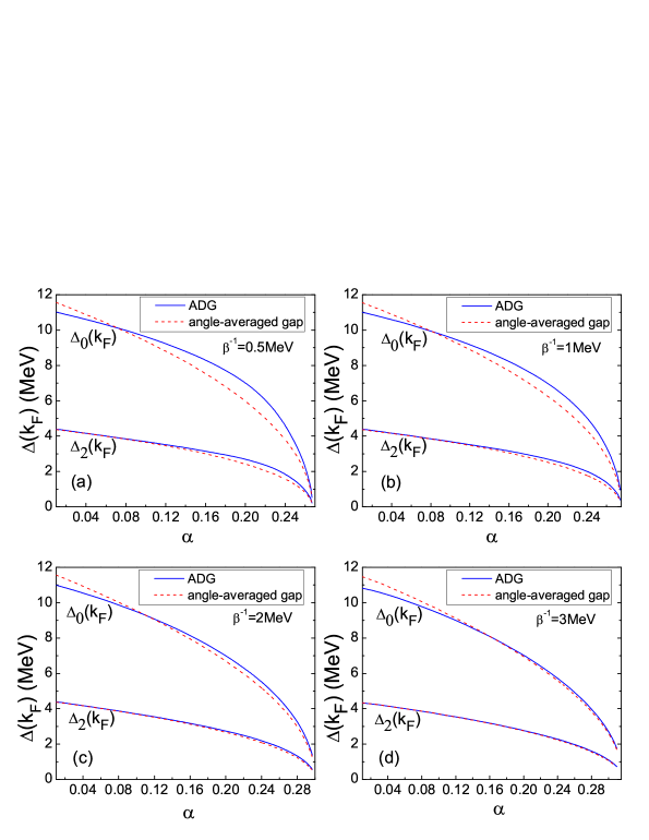
Figure 1: (Color online). The upper and lower curves in the figures are related to the values of $\Delta_{0}(k_{F})$ and $\Delta_{2}(k_{F})$ vs isospin-asymmetry $\alpha$. The blue solid and red dashed lines correspond to the ADG and angle-averaged gap, respectively.

Fig.1 shows the angle-averaged and angle dependent gaps $\Delta_{0}(k_{F})$ and $\Delta_{2}(k_{F})$ in the ${}^{3}SD_{1}$ partial-wave channel as a function of isospin-asymmetry $\alpha$, defined as $\alpha=(\rho_{n}-\rho_{p})/\rho$. The temperatures are set at low-temperature regime $\beta^{-1}=$ $0.5$ MeV, $1.0$ MeV, $2.0$ MeV, $3.0$ MeV (the critical temperature $\beta^{-1}_{c}$ where the superfluid vanishes is about $7.5$ MeV for isospin-symmetric case). At temperature $\beta^{-1}=0.5$ MeV, the value of $\Delta_{0}(k_{F})$ in the ADG state becomes larger than that of the angle-averaged gap state for $\alpha\geq 0.07$, and the difference of $\Delta_{0}(k_{F})$ between the ADG and angle-averaged gap states reaches 22 percent at $\alpha=0.23$. With increasing temperature, the difference of $\Delta_{0}(k_{F})$ between the two kinds of states decreases rapidly. The critical isospin-asymmetries $\alpha_{c}$ at which the gaps vanish are the same in the two states, and their values are $0.267$, $0.275$, $0.30$ and $0.315$ for the temperatures $0.5$ MeV, $1.0$ MeV, $2.0$ MeV and $3.0$ MeV, respectively. It implies that the thermal excitation can promote pairing in large isospin-asymmetry nuclear matter at low temperature regime.

In order to have an entire inspection of the difference between the pairing gaps of the ADG state and the angle-averaged gap state, we exhibit the gap functions in Fig.2.

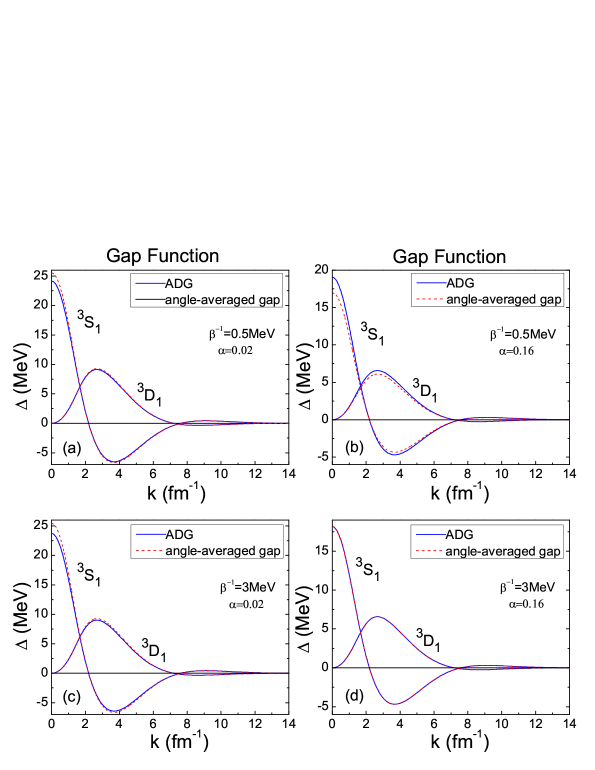
Figure 2: (Color online). The curves marked with symbols ${}^{3}S_{1}$ and ${}^{3}D_{1}$ are related to the gap functions $\Delta_{0}(k)$ and $\Delta_{2}(k)$ in Eqs.(24) and (30). The blue solid and red dashed lines correspond to the ADG and angle-averaged gap, respectively.

At temperature $\beta^{-1}=0.5$ MeV, the gap functions of the two different kinds of states are almost the same except a little difference of $\Delta_{0}(k)$ near the zero momentum for the asymmetry $\alpha=0.02$ [in Fig.2.(a)]. When the system becomes more asymmetric, the difference gets larger [in Fig.2.(b)]. However, the curves of the ADG coincide with these of the angle-averaged gap for $\beta^{-1}=3.0$ MeV with $\alpha=0.16$ [in Fig.2.(d)]. That implies the angle-averaging procedure is a satisfactory approximation for asymmetric nuclear matter at high temperatures.

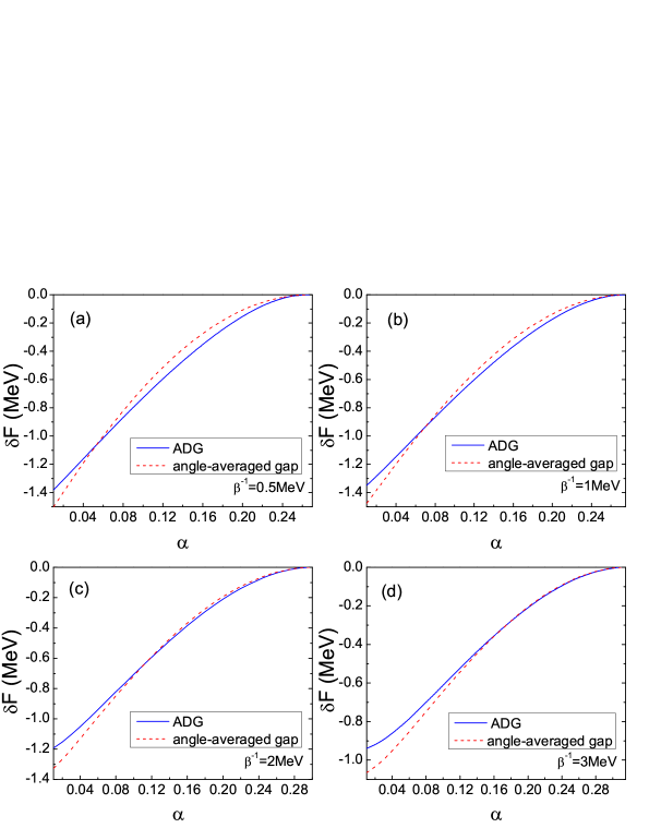
Figure 3: (Color online). The difference of the free energy between the superconducting and normal states as a function of the isospin-symmetry $\alpha$ for diffderent temperatures. The blue solid and red dashed lines correspond to the ADG and angle-averaged gap, respectively.

A larger gap value in ADG state may result in a larger pairing energy in the condensate [second term in Eqs.(36) and (37)], which has important influence on the free energy of the superconducting state. Thus we calculate the free-energy difference $\delta\emph{F}$ between the normal and superconducting states. The results are shown in Fig.3, where the parameters are set as the same as those in Fig.1. At temperature $\beta^{-1}=0.5$ MeV, $\delta F$ in the ADG state gets smaller than that of the angle-averaged gap state when $\alpha\geq 0.06$, especially, the former is about 35 percent lower than the latter in the regime $\alpha>0.17$. We can conclude that the ADG state is more favored than the angle-averaged gap state for large asymmetry at low temperature, since the angle dependence of the pairing gap enhances the pairing energy and has little effect on the kinetic energy. However, the thermal excitation can reduce the effects of angle dependence of the pairing gap [comparing the Fig.3.(a) with Fig.3.(d)]. It is also shown in Fig.3 that the values of $\delta F$ tend to zero gently when $\alpha\rightarrow\alpha_{c}$ at different temperatures.

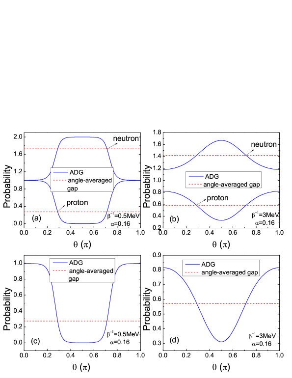
Figure 4: (Color online). The higher and lower curves in the upper two figures are related to the neutron and proton occupation probabilities, respectively. The curves in the lower two figures are the pairing probabilities. The blue solid and red dashed lines correspond to the ADG and angle-averaged gap, respectively.

One straightforward way to understand the effects of angle dependence of the pairing gap is to investigate the normal and superconducting occupation probabilities [obtained from Eqs.(14) and (15)] near the average Fermi surface (related to the average chemical potential of neutron and proton). The results are depicted in Fig.4, where the spin summation has been carried out. In this figure, the neutron/proton and pairing particle occupation probabilities at the average Fermi surface for a fixed asymmetry $\alpha=0.16$ at temperature $\beta^{-1}=$ $0.5$ MeV has been compared with those at $3.0$ MeV. In isospin-asymmetric nuclear matter, the large splitting between the neutron and proton occupation probabilities prevents the pairing around the average Fermi surface in the angle-averaging procedure. However, in the ADG state, the splitting is reduced by the angle dependence of the pairing gap in partial area around the average Fermi surface, i.e., in the regime $\theta\subset(0,\frac{\pi}{5})\cup(\frac{4\pi}{5},\pi)$ as shown in Fig.4.(a). In Fig.4.(c), as compared with the angle-averaged gap, although the pairing in the ADG state is almost fully suppressed in the regime $\theta\subset(\frac{\pi}{5},\frac{4\pi}{5})$ in ADG state, it is obviously enhanced at $\theta$ smaller than $\frac{\pi}{5}$ and greater than $\frac{4\pi}{5}$.

Substituting the expression of $D^{2}(\textbf{k})$ in Eq.(31) into Eq.(14), we can find that the Fermi spheres of neutron and proton are no longer isotropic in the ADG state. Since we assume an axi-symmetric quasiparticle spectrum in the ADG state, the rotational symmetry is spontaneously broken [in terms of group theory the $O(3)$ symmetry breaks down to $O(2)$] and there exists one favored direction. The neutron Fermi sphere possesses an oblate deformation perpendicular to the favored direction, whereas the proton Fermi sphere has a prolate deformation along the favored direction. The two different deformations enhance the correlation between neutrons and protons near their average Fermi surface. However, at high temperature the neutron/proton occupation probability in the ADG becomes almost isotropic as shown in Fig.4.(b), namely, the thermal excitation reduces the angle dependence of quasiparticle spectra. In this case, the deformation of the neutron/proton Fermi sphere fails to increase the phase-space overlap of neutron and proton near their average Fermi surface effectively. Thus the results of the ADG state are nearly the same as that of the angle-averaged gap state, i.e., the angle-averaging procedure becomes an adequate approximation at high temperatures $\beta^{-1}\geq 3$ MeV.

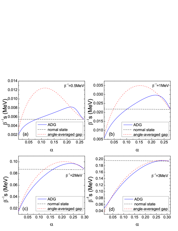
Figure 5: (Color online). The entropy (scaled by $\beta^{-1}$) as a function of the isospin-symmetry $\alpha$ for different temperature. The blue solid, red dashed and black dash-dotted lines correspond to the ADG, angle-averaged gap and normal state, respectively.

Fig.5 displays the entropy ($\beta^{-1}S$) as a function of isospin-asymmetry $\alpha$ for different temperatures $\beta^{-1}=$ $0.5$ MeV, $1.0$ MeV, $2.0$ MeV and $3.0$ MeV. The entropy in the superconducting state is smaller than that in the normal state near $\alpha=0$, and gets larger than that in the normal state at sufficiently large asymmetry. However, around the transition point $\alpha_{c}$ from the superconducting state to the normal state, the entropies of the superconducting states (both of the ADG state and the angle-averaged gap state) approach to the value of the normal state, i.e., the latent heats $Q=\beta^{-1}(S_{s}-S_{n})\rightarrow 0$ when $\alpha\rightarrow\alpha_{c}$. Hence the transitions are of second order. At temperature $\beta^{-1}=$ $0.5$ MeV, the entropy in the ADG state is nearly a linear function of the isospin-asymmetry when $0.02<\alpha<0.22$. With increasing temperature, the linear property of the entropy curve disappears and the difference between the ADG state and the angle-averaged gap state gets smaller.

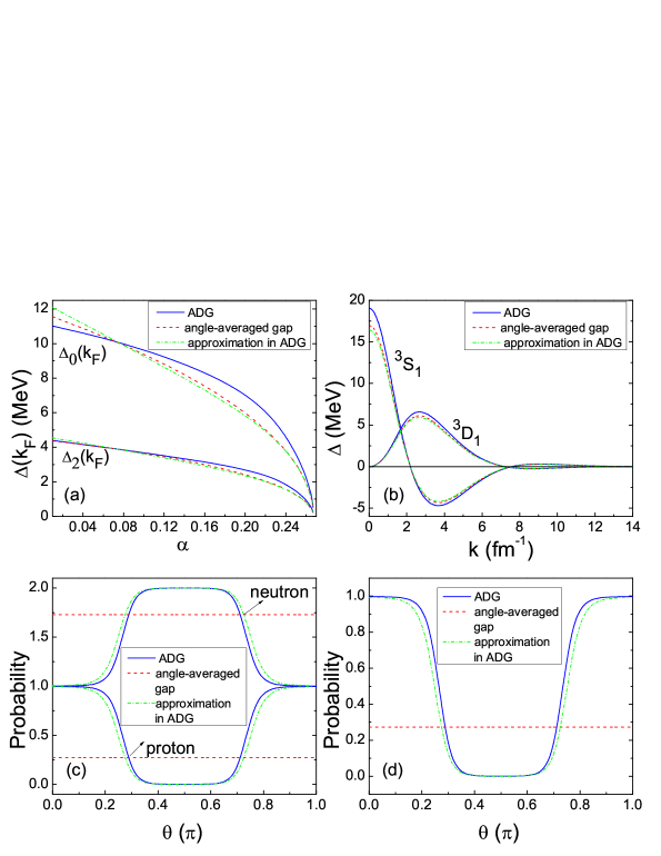
Figure 6: (Color online). $\Delta_{0}(k_{F})$ and $\Delta_{2}(k_{F})$ as a function of isospin-asymmetry $\alpha$ for the ADG, angle-averaged gap and `approximation in ADG' are shown in Fig.(a). Fig.(b) exhibits the gap functions for the three case. The normal and superconducting occupation probabilities at the average Fermi surface for the three case are shown in Figs.(c) and (d), respectively. The blue solid, red dashed and green dash-dotted lines correspond to the ADG, angle-averaged gap and the `approximation in ADG', respectively. The temperature is set to be $\beta^{-1}=0.5$ MeV, and the isospin-asymmetry $\alpha=0.16$ in (b), (c), (d).

Comparing the gap equations (30) for the ADG state with Eq.(24) for the angle-averaged gap state, two differences appear in the ADG state, i.e., the angle dependent quasiparticle spectrum and the angle matrix $\left(\begin{array}[]{ll}\emph{f}(\theta)&\emph{g}(\theta)\\ \emph{g}(\theta)&\emph{h}(\theta)\end{array}\right)$. The first leads to the deformation of neutron/proton Fermi sphere, and the second corresponds to the coupling among different $m_{j}$ gap components. Actually, the angle matrix modifies the strength of $V^{l^{{}^{\prime}}l}_{\lambda}(k^{{}^{\prime}},k)$ in different directions in momentum space. We replace the angle matrix by $\frac{1}{4\pi}\left(\begin{array}[]{ll}1&0\\ 0&1\end{array}\right)$ to inspect the influence of the angle matrix. The results are shown in Fig.6 for asymmetry $\alpha=0.16$ in (b), (c), (d) and the temperature is set to be $\beta^{-1}=0.5$ MeV. The dash-doted lines denoted by `approximation in ADG' are obtained by replacing the angle matrix with $\frac{1}{4\pi}\left(\begin{array}[]{ll}1&0\\ 0&1\end{array}\right)$. Figs.6.(c) and (d) exhibit the neutron/proton and pairing particle occupation probabilities at the average Fermi surface, respectively. The curves of ADG and `approximation in ADG' are nearly the same in Figs.6.(c) and (d). Whereas the gap functions in Fig.6.(b) show that the curves of `approximation in ADG' behave closer to those of the angle-averaged gap state than those of the ADG state. Fig.6.(a) displays the $\Delta_{0}(k_{F})$ and $\Delta_{2}(k_{F})$ vs isospin-asymmetry $\alpha$. The gaps of `approximation in ADG' turn out to be smaller than both the gaps in the ADG state and angle-averaged gap state when $\alpha>0.07$. Moreover, the curves of `approximation in ADG' are much closer to that of the angle-averaged gap state. All these results indicate that the influence of the angle matrix is much more important than that of the angle dependence of quasiparticle spectrum. Furthermore, the coupling from different $m_{j}$ gap components may strengthen the pairing interaction for large isospin-asymmetry at low temperatures.

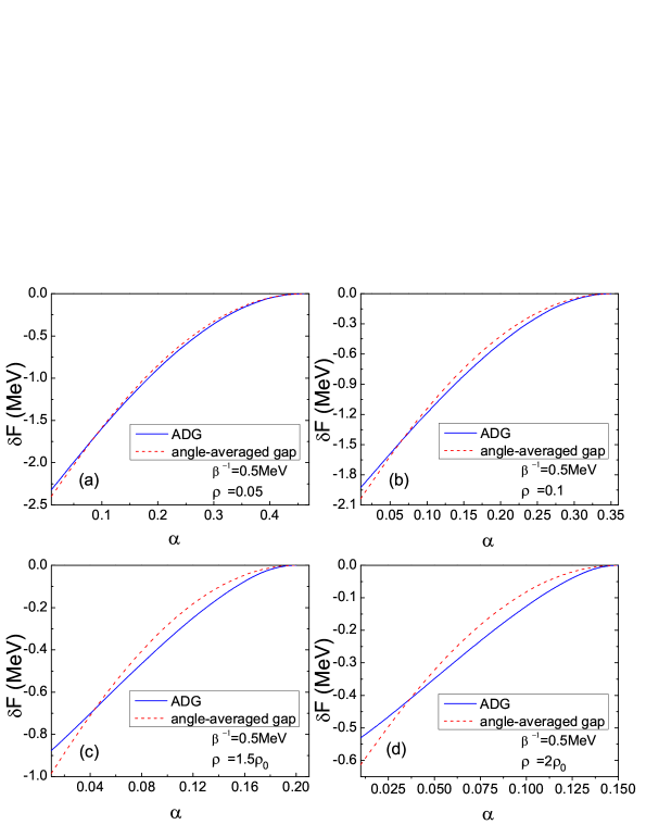
Figure 7: (Color online). The difference of the free energy between the superconducting and normal states as a function of the isospin-symmetry $\alpha$ for different densities at a fixed temperature $\beta^{-1}=0.5$ MeV. The blue solid and red dashed lines correspond to the ADG and angle-averaged gap, respectively.

In order to discuss the effect of angle dependence of the pairing gap for different densities, we show the free energy difference $\delta\emph{F}$ between the superconducting and normal states at temperature $\beta^{-1}=0.5$ MeV vs isospin-asymmetry $\alpha$ in Fig.7. The densities are set to be $\rho=0.05$, $0.1$, $1.5\rho_{0}$ and $2\rho_{0}$ for (a), (b), (c) and (d), respectively. At the density $\rho=0.05$ [in Fig.7.(a)], the two curves of $\delta\emph{F}$ for the ADG and angle-averaged gap states are very close to each other, indicating the effect of angle dependence of the pairing gap is quite small at low densities. When the density increases, the difference of $\delta\emph{F}$ for the ADG and angle-averaged gap states increases rapidly, implying that the angle dependence of the pairing gap is more important at higher densities. As the Fermi energy $\emph{E}_{F}\propto\rho^{\frac{2}{3}}$, the value of $\frac{\Delta}{\emph{E}_{F}}$ is thus small at high densities. In this case, the summations over ${k}^{{}^{\prime}}$ in the gap equation (9) concentrate near the average Fermi surface (i.e., the contribution to superfluidity from the Cooper pairs around the average Fermi surface is dominant). A little separation of the neutron and proton Fermi surfaces $\delta\mu$ may suppress the superfluidity strongly. In the ADG configuration, the angle dependence can reduce the suppression. However, at low densities, the value of $\frac{\Delta}{\emph{E}_{F}}$ gets large. Thus the contribution to superfluidity from the Cooper pairs near the average Fermi surface is no longer as important as that at high densities. Since the angle dependence mainly increases the pairing probability around the average Fermi surface, the effect of the angle dependence becomes weak at low densities.

IV Summary and Outlook

The fermionic condensation in asymmetric nuclear matter leads to superconducting states which spontaneously break the spatial symmetries (such as FFLO and DFS states). The quasiparticle spectrum behaves as an isotropic one and the angle dependence of the pairing gap should be reconsidered. In this work we propose an axi-symmetric angle dependent gap state in which the isotropic symmetry is broken in isospin-asymmetric nuclear matter, and compare with the angle-averaged gap state. It is shown the ADG state is more favored than the angle-averaged gap state for large asymmetry at low temperature, and the differences of both the gap values and the free energies between the two kinds of states get small with increasing temperature. At temperature $\beta^{-1}=0.5$ MeV with density $\rho_{0}$, the maximal differences of $\Delta_{0}(k_{F})$ and $\delta\emph{F}$ between the ADG state and angle-averaged gap state are about 22 and 35 percent, respectively. The differences get larger at higher densities for $\beta^{-1}=0.5$ MeV. In the ADG state, the neutron and proton deformed Fermi spheres increase the pairing probability along the axis of symmetry breaking near their average Fermi surface. The effect of the coupling among different $m_{j}$ gap components is also investigated in this work and we find the coupling dominates the main contribution to the mechanism of the ADG state.

The ADG state vanishes at the critical value $\alpha_{c}$, where the angle-averaged gap vanishes. And the phase transition from the ADG state to the normal state is of the second order. When temperature goes up, $\alpha_{c}$ rises and the effect of angle dependence of pairing gap becomes weak. In a certain region of $\alpha$ the latent heat has an anomalous negative sign, which is consistent with the result if Ref.Sdd2 . However, this does not affect the stability of the ADG state, since its energy budget is dominated by the pair-condensation energy.

In the ADG state, the symmetry is broken spontaneously. It is different from that in the FFLO state, where the symmetry is broken by the collective motion of the cooper pairs (the translation and rotational symmetries are both broken). The translation symmetry is maintained in the ADG state. The deformation of the neutron/proton Fermi sphere in the ADG state is similar to the DFS configuration, however, the mechanisms are different. In the DFS state the symmetry breaking corresponds to the deformed Fermi surface, while in the ADG state the symmetry breaking results from the angle dependence of the pairing gap. As is well known, the continuous symmetry breaking leads to collective excitations with vanishing minimal frequency (Goldstone's theorem). The breaking of rotational symmetry, which corresponds to the anisotropic $D^{2}(\textbf{k})$ in the ADG state, may imply new collective bosonic modes in asymmetric nuclear matter. However, the true ground state could be a combination of the ADG state and the FFLO state, we should consider the ADG state with the cooper pair momentum together which is in progress.

Appendix

We present here the main steps of the elimination of the second term in Eq.(36) by using the gap equation (9). The elements of the density matrix of the particles in condensate are,

$$\nu_{\sigma_{1},\sigma_{2}}(\textbf{k})=\frac{\Delta_{\sigma_{1},\sigma_{2}}(\textbf{k})}{2\sqrt{\xi_{\textbf{k}}^{2}+D^{2}(\textbf{k})}}[1-f(E_{\textbf{k}}^{+})-f(E_{\textbf{k}}^{-})].$$ (54)

The second term of Eq.(36) is written as

$$\sum_{\textbf{k},\textbf{k}^{{}^{\prime}}}\sum_{\sigma_{1},\sigma_{2},\sigma_{1}^{{}^{\prime}},\sigma_{2}^{{}^{\prime}}}<\textbf{k}\sigma_{1},-\textbf{k}\sigma_{2}\mid V\mid\textbf{k}^{{}^{\prime}}\sigma_{1}^{{}^{\prime}},-\textbf{k}^{{}^{\prime}}\sigma_{2}^{{}^{\prime}}>\nu^{{\dagger}}_{\sigma_{2},\sigma_{1}}(\textbf{k})\nu_{\sigma_{1}^{{}^{\prime}},\sigma_{2}^{{}^{\prime}}}(\textbf{k}^{{}^{\prime}})$$

$$=\sum_{\textbf{k},\textbf{k}^{{}^{\prime}}}\sum_{\sigma_{1},\sigma_{2},\sigma_{1}^{{}^{\prime}},\sigma_{2}^{{}^{\prime}}}<\textbf{k}\sigma_{1},-\textbf{k}\sigma_{2}\mid V\mid\textbf{k}^{{}^{\prime}}\sigma_{1}^{{}^{\prime}},-\textbf{k}^{{}^{\prime}}\sigma_{2}^{{}^{\prime}}>\frac{\Delta^{{\dagger}}_{\sigma_{2},\sigma_{1}}(\textbf{k})}{2\sqrt{\xi_{\textbf{k}}^{2}+D^{2}(\textbf{k})}}[1-f(E_{\textbf{k}}^{+})-f(E_{\textbf{k}}^{-})]$$

$$\times\frac{\Delta_{\sigma_{1}^{{}^{\prime}},\sigma_{2}^{{}^{\prime}}}(\textbf{k}^{{}^{\prime}})}{2\sqrt{\xi_{\textbf{k}^{{}^{\prime}}}^{2}+D^{2}(\textbf{k}^{{}^{\prime}})}}[1-f(E_{\textbf{k}^{{}^{\prime}}}^{+})-f(E_{\textbf{k}^{{}^{\prime}}}^{-})]$$

$$=\sum_{\textbf{k},\sigma_{1},\sigma_{2}}\frac{\Delta^{{\dagger}}_{\sigma_{2},\sigma_{1}}(\textbf{k})}{2\sqrt{\xi_{\textbf{k}}^{2}+D^{2}(\textbf{k})}}[1-f(E_{\textbf{k}}^{+})-f(E_{\textbf{k}}^{-})]$$

$$\times\sum_{\textbf{k}^{{}^{\prime}},\sigma_{1}^{{}^{\prime}},\sigma_{2}^{{}^{\prime}}}<\textbf{k}\sigma_{1},-\textbf{k}\sigma_{2}\mid V\mid\textbf{k}^{{}^{\prime}}\sigma_{1}^{{}^{\prime}},-\textbf{k}^{{}^{\prime}}\sigma_{2}^{{}^{\prime}}>\frac{\Delta_{\sigma_{1}^{{}^{\prime}},\sigma_{2}^{{}^{\prime}}}(\textbf{k}^{{}^{\prime}})}{2\sqrt{\xi_{\textbf{k}^{{}^{\prime}}}^{2}+D^{2}(\textbf{k}^{{}^{\prime}})}}[1-f(E_{\textbf{k}^{{}^{\prime}}}^{+})-f(E_{\textbf{k}^{{}^{\prime}}}^{-})].$$ (55)

Noting that the second summation over ${k}^{{}^{\prime}},\sigma_{1}^{{}^{\prime}},\sigma_{2}^{{}^{\prime}}$ is $-\Delta_{\sigma_{2},\sigma_{1}}$ (using the gap equation (9)), thus

$$\sum_{\textbf{k},\textbf{k}^{{}^{\prime}}}\sum_{\sigma_{1},\sigma_{2},\sigma_{1}^{{}^{\prime}},\sigma_{2}^{{}^{\prime}}}<\textbf{k}\sigma_{1},-\textbf{k}\sigma_{2}\mid V\mid\textbf{k}^{{}^{\prime}}\sigma_{1}^{{}^{\prime}},-\textbf{k}^{{}^{\prime}}\sigma_{2}^{{}^{\prime}}>\nu^{{\dagger}}_{\sigma_{2},\sigma_{1}}(\textbf{k})\nu_{\sigma_{1}^{{}^{\prime}},\sigma_{2}^{{}^{\prime}}}(\textbf{k}^{{}^{\prime}})$$

$$=-\sum_{\textbf{k},\sigma_{1},\sigma_{2}}\frac{\Delta^{{\dagger}}_{\sigma_{2},\sigma_{1}}(\textbf{k})\Delta_{\sigma_{1},\sigma_{2}}(\textbf{k})}{2\sqrt{\xi_{\textbf{k}}^{2}+D^{2}(\textbf{k})}}[1-f(E_{\textbf{k}}^{+})-f(E_{\textbf{k}}^{-})]$$

$$=-\sum_{\textbf{k}}\frac{Tr[\Delta(\textbf{k})\Delta^{{\dagger}}(\textbf{k})]}{2\sqrt{\xi_{\textbf{k}}^{2}+D^{2}(\textbf{k})}}[1-f(E_{\textbf{k}}^{+})-f(E_{\textbf{k}}^{-})].$$ (56)

Using the ``unitary" property Eq.(4),

U $$=\sum_{\sigma\textbf{k}}[\varepsilon_{\textbf{k}}^{(n)}n_{\sigma}^{(n)}(\textbf{k})+\varepsilon_{\textbf{k}}^{(p)}n_{\sigma}^{(p)}(\textbf{k})]$$ (57)

$$+\sum_{\textbf{k},\textbf{k}^{{}^{\prime}}}\sum_{\sigma_{1},\sigma_{2},\sigma_{1}^{{}^{\prime}},\sigma_{2}^{{}^{\prime}}}<\textbf{k}\sigma_{1},-\textbf{k}\sigma_{2}\mid V\mid\textbf{k}^{{}^{\prime}}\sigma_{1}^{{}^{\prime}},-\textbf{k}^{{}^{\prime}}\sigma_{2}^{{}^{\prime}}>\nu^{{\dagger}}_{\sigma_{2},\sigma_{1}}(\textbf{k})\nu_{\sigma_{1}^{{}^{\prime}},\sigma_{2}^{{}^{\prime}}}(\textbf{k}^{{}^{\prime}})$$

$$=\sum_{\sigma\textbf{k}}[\varepsilon_{\textbf{k}}^{(n)}n_{\sigma}^{(n)}(\textbf{k})+\varepsilon_{\textbf{k}}^{(p)}n_{\sigma}^{(p)}(\textbf{k})]-\sum_{\textbf{k}}\frac{2D^{2}(\textbf{k})}{2\sqrt{\xi_{\textbf{k}}^{2}+D^{2}(\textbf{k})}}[1-f(E_{\textbf{k}}^{+})-f(E_{\textbf{k}}^{-})]$$

$$=\sum_{\sigma\textbf{k}}[\varepsilon_{\textbf{k}}^{(n)}n_{\sigma}^{(n)}(\textbf{k})+\varepsilon_{\textbf{k}}^{(p)}n_{\sigma}^{(p)}(\textbf{k})]-\sum_{\textbf{k}}\frac{D^{2}(\textbf{k})}{\sqrt{\xi_{\textbf{k}}^{2}+D^{2}(\textbf{k})}}[1-f(E_{\textbf{k}}^{+})-f(E_{\textbf{k}}^{-})].$$

References

- (1)
- (2) A.L.Goodman, Phys. Rev. C 60, 014311 (1999), and references therein.
- (3) G.Röpke, A.Schnell, P.Schuck, and U.Lombardo, Phys. Rev. C 61, 024306 (2000).
- (4) Th.Alm, B.L.Friman, G.Röpke, and H.Schulz, Nucl. Phys. A 551, 45 (1993).
- (5) M.Baldo, U.Lombardo, P.Schuck, Phys. Rev. C 52, 975 (1995).
- (6) E.Garrido, P.Sarriguren, E.Moya de Guerra, and P.Schuck, Phys. Rev. C 60, 064312 (1999).
- (7) A.Sedrakian, Th.Alm, U.Lombardo, Phys. Rev. C 55, R582 (1997).
- (8) A.Sedrakian, U.Lombardo, Phys. Rev. Lett. 84, 602 (2000).
- (9) U.Lombardo, P.Nozieres, P.Schuck, H.J.Schulze, A.Sedrakian, Phys. Rev. C. 64, 064314 (2001).
- (10) Ø.Elgaroy, L.Engvik, M.Hjorth-Jensen, and E.Osnes, Phys. Rev. C. 57, R1069 (1998).
- (11) A.I.Akhiezer, A.A.Isayev, S.V.Peletminsky, and A.A.Yatsenko, Phys. Rev. C. 63, 021304 (2001).
- (12) A.Sedrakian, G.Röpke, T.Alm, Nucl. Phys. A 594, 355 (1995).
- (13) T.Alm, G.Röpke, A.Sedrakian, and F.Weber, Nucl. Phys. A 604, 491 (1996).
- (14) S.Typel, G.Röpke, T.Klähn, D.Blaschke, and H.H.Wolter, Phys. Rev. C. 81, 015803 (2010).
- (15) S.Heckel, P.P.Schneider, and A.Sedrakian, Phys. Rev. C. 80, 015805 (2009).
- (16) M.Stein, X.-G.Huang, A.Sedrakian, and J.W.Clark, Phys. Rev. C. 86, 062801 (2012).
- (17) P. Fulde and R. A. Ferrell, Phys. Rev. 135 (1964) A550.
- (18) A. I. Larkin and Yu. N. Ovchinnikov, Zh. Eksp. Teor. Fiz. 47 (1964) 1136 [translation, Sov. Phys. JETP 20 (1965) 762].
- (19) H.Müther, and A.Sedrakian, Phys. Rev. Lett. 88, 252503 (2002).
- (20) A.Sedrakian, Phys. Rev. C. 63, 025801 (2001).
- (21) H.Müther, and A.Sedrakian, Phys. Rev. C. 67, 015802 (2003).
- (22) M.Baldo, I.Bombaci, and U.Lombardo, Phys. Lett. B. 283, 8 (1992).
- (23) M.Baldo, J.Cugnon, A.Lejeune, and U.Lombardo, Nucl. Phys. A 536 349 (1992).
- (24) U.Lombardo, H.-J.Schulze, and W. Zuo, Phys. Rev. C. 59, 2927 (1999).
- (25) M.Baldo, U.Lombardo, H.-J.Schulze, and Zuo Wei, Phys. Rev. C. 66, 054304 (2002).
- (26) Caiwan Shen, U.Lombardo, P.Schuck, Phys. Rev. C. 71, 054301 (2005).
- (27) L. G. Cao, U.Lombardo, P.Schuck, Phys. Rev. C. 74, 064301 (2006).