from 1st Sept: ] Mathematical Institute, University of Oxford, OX1 3LB, UK

Dynamical Systems to Monitor Complex Networks in Continuous Time

Abstract

In many settings it is appropriate to treat the evolution of pairwise interactions over continuous time. We show that new Katz-style centrality measures can be derived in this context via solutions to a nonautonomous ODE driven by the network dynamics. This allows us to identify and track, at any resolution, the most influential nodes in terms of broadcasting and receiving information through time dependent links. In addition to the classical notion of attenuation across edges used in the static Katz centrality measure, the ODE also allows for attenuation over time, so that real time “running measures” can be computed. With regard to computational efficiency, we explain why it is cheaper to track good receivers of information than good broadcasters. We illustrate the new measures on a large scale voice call network, where key features are discovered that are not evident from snapshots or aggregates.

Many systems of interacting agents involve transient edges, and this time-dependency raises a variety of challenges Holme and Saramäki (2012). Currently, the dominant paradigm is to consider activity over time-windows, and hence to deal with network snapshots over discrete time. This approach is useful for modeling both the evolution of the underlying connectivity and the dynamics of processes over the network Barrat et al. (2013); Lambiotte et al. (2011); Stehlé et al. (2011). The idea of viewing the network as a time-ordered sequence of sparse adjacency matrices is also extremely convenient for data-driven analysis Grindrod et al. (2011); Grindrod and Higham (2013); Tang et al. (2010a); Lentz et al. (2013); Mucha et al. (2010); Tang et al. (2010b). More generally, abstracting from time to any countable index representing possible levels in a hierarchy (such as gene/mRNA/protein) we arrive at multiplex networks Gómez et al. (2013), which can be usefully viewed as multidimensional tensors Dunlavy et al. (2011).

However, in many settings using a time-ordered sequence of network snapshots forces us to make awkward compromises. On one hand, by taking the time window too large we lose the ability to reproduce high-frequency transient behaviour, where an edge switches on and off multiple times in the space of a single window. On the other hand, time points that are too finely spaced can lead to redundant, empty windows that waste computational effort. Very short time windows may also lead to a false impression of accuracy—for remote interactions such as emails and tweets, although there is an unambiguous and instantaneous time at which information was sent, the time at which the receiver (a) digests and then, possibly, (b) acts upon the information is generally not recordable.

In this work we will show that it is possible to extract insight directly from an adjacency matrix defined as a function of continuous time. We focus on the computationally-motivated task of monitoring the influence of nodes in a given network. However, we note that the ODE setting developed here also has potential for high-level analysis and prediction, since the tools of dynamical systems become available when network models are combined with the centrality evolution; for example, via a law of social balance Marvel et al. (2011); Traag et al. (2013) or triadic closure Grindrod et al. (2012). Hence, there is potential to study the evolution of centrality under various network “laws of motion” and to compare predictions from competing models.

For a fixed set of $N$ nodes, we let $A(t)$ denote the state of the network at time $t$. In the case of voice call data, it is natural for the entries in the adjacency matrix to be discontinuous, binary-valued, functions of time, switching on to 1 and off to 0 when an exchange starts and finishes, respectively. So in this case each $A(t)\in\mathbb{R}^{N\times N}$ is binary and symmetric with $A_{ij}(t)=A_{ji}(t)=1$ if and only if nodes $i$ and $j$ are in communication at time $t$. (To be concrete, and without loss of generality, we will assume continuity from the right.) For social interactions such as emails and tweets, this methodology allows us to spike the relevant edge when a message is sent out, and then, as $t$ increases, let the value to decay towards zero—this reflects the fact that these exchanges have a natural delay, and also that messages lose their impact and visibility over time. In this case $A(t)$ is generally unsymmetric, taking values between zero and one.

Our aim is now to generate a real-valued, unsymmetric dynamic communicability matrix $S(t)\in\mathbb{R}^{N\times N}$ such that $S(t)_{ij}$ quantifies the ability of node $i$ to communicate with node $j$ up to time $t$, that is, by making use of edges that have appeared at time $t$ or earlier. We propose that $S(t)$ is updated over a small time interval $\delta t$ according to

$$S(t+\delta t)=\left(I+e^{-b\delta t}S(t)\right)\left(I-aA(t+\delta t)\right)^{-\delta t}-I,$$ (1)

with $S(0)=0$. Here, $I\in\mathbb{R}^{N\times N}$ denotes the identity matrix, and $a,b>0$ are parameters. To justify this new iteration and explain the role of the parameters, suppose first that $\delta t=1$, and we are therefore given access to the adjacency matrix only on a fixed grid of timepoints. In the extreme case of a single timepoint, (1) reduces to $S(1)+I=(I-aA(1))^{-1}$. This corresponds to the classical static network analysis measure of Katz Katz (1953); for $i\neq j$, $S(1)_{ij}$ counts the total number of distinct walks through the network from node $i$ to node $j$, with walks of length $k$ downweighted by $a^{k}$. The attenuation factor $a$ may be interpreted as the probability that a message successfully traverses an edge. With multiple time points and $b=0$ in (1) we have

$$S(N)+I = \left(I-aA(1)\right)^{-1}\left(I-aA(2)\right)^{-1}\cdots$$ (2)

$$\mbox{}~{}~{}~{}~{}~{}~{}~{}~{}~{}~{}~{}~{}~{}~{}~{}~{}~{}~{}~{}~{}~{}~{}~{}~{}\left(I-aA(N)\right)^{-1}.$$

It was shown in Grindrod et al. (2011) that this iteration generalizes the Katz centrality measure to the case of a time-ordered network sequence. Here $S(N)_{ij}$ records an edge-downweighted count of the total number of distinct dynamic walks through the network, where a dynamic walk is any traversal that respects the time-ordering of the edges. We note that the same idea was later used to define concept of accessibility Lentz et al. (2013). The general case of (1) with $b>0$ and $\delta t=1$ was introduced in Grindrod and Higham (2013), where it was shown that the parameter $b$ plays the role of downweighting for time—walks that began $k$ time units ago are scaled by $e^{-bk}$. This temporal scaling is designed to take account of the fact that older messages generally have less current relevance.

A key step in writing down the new iteration (1) was to devise a scaling under which the $\delta t\to 0$ limit is meaningful. Our choice of a $\delta t$-dependent power in the matrix products can be explained by focusing on the $b=0$ case over a short time interval. If we refine from the single interval $[t,t+\delta t]$ to the pair of intervals $[t,t+\delta t/2]$ and $[t+\delta t/2,t+\delta t]$ and consider the scenario where $A(t)$ does not change, the simple identity

$$\left(I-aA(t)\right)^{-{\scriptstyle{{\frac{1}{2}}}}\delta t}\left(I-aA(t)\right)^{-{\scriptstyle{{\frac{1}{2}}}}\delta t}=\left(I-aA(t)\right)^{-\delta t}$$

shows that our scaling produces consistent results.

For convenience, we will let $U(t)=I+S(t)$ in taking the $\delta t\to 0$ limit. We then write (1) in the form

$$U(t+\delta t) = \left(I+e^{-b\delta t}\left(U(t)-I\right))\right)$$

$$\mbox{}\times\exp\left(-\delta t\log\left(I-aA(t+\delta t)\right)\right),$$

where $\exp$ and $\log$ denote the matrix exponential and logarithm respectively, and we have used the identities $H=e^{\log H}$ and $\log(H^{\alpha})=\alpha\log H$ for $-1\leq\alpha\leq 1$; see, for example, Higham (2008). Expanding and taking the limit $\delta t\to 0$ we then arrive at the matrix ODE

$$U^{\prime}(t)=-b\left(U(t)-I\right)-U(t)\log\left(I-aA(t)\right),$$ (3)

with $U(0)=I$.

In order to focus on nodal properties, we can take row and column sums in the matrix $U(t)$ to define the dynamic broadcast and dynamic receive vectors

$${\bf b}(t)=U(t)\mathbf{1}\quad\mathrm{and}\quad{\bf r}(t)=U(t)^{T}\mathbf{1},$$ (4)

where $\mathbf{1}\in\mathbb{R}^{N}$ denotes the vector of ones. Here, ${\bf b}_{i}(t)$ and ${\bf r}_{i}(t)$ measure the current propensity for node $i$ to have broadcasted and received information, respectively, across the dynamic network, under our assumptions that longer and older walks have less relevance.

It is interesting to note from (3) that the receive centrality satisfies its own vector-valued ODE

$${\bf r}^{\prime}(t)=-b\left(r(t)-\mathbf{1}\right)-\left(\log\left(I-aA(t)\right)\right)^{T}{\bf r}(t),$$

with ${\bf r}(0)=\mathbf{1}$, which is a factor of $N$ smaller in dimension than (3) and hence cheaper to simulate. By contrast, it is not possible to disentangle the broadcast centrality in this way. Intuitively, this difference arises because the node-based receive vector ${\bf r}(t)$ keeps track of the overall level of information flowing into each node, and this can be propagated forward in time as new links become available. However, the broadcast vector ${\bf b}(t)$ keeps track of information that has flowed out of each node—we do not record where the information currently resides and hence we cannot update based on ${\bf b}(t)$ alone. So, with this methodology, real time updating of the receive centrality is fundamentally simpler than real time updating of the broadcast centrality.

The choice of downweighting parameters, $a$ and $b$, clearly plays an important role, and should depend to a large extent on the nature of the interactions represented by $A(t)$. The temporal downweighting parameter, $b$, has the natural interpretation that walks starting $t$ time units ago are downweighted by $e^{-bt}$, so $b$ allows us summarize the rate at which news goes stale. Hence $b$ could be calibrated by studying the typical half-life of a link Bilton (2011).

For the edge-attenuation parameter, $a$, in the discrete iteration (2) there is a natural upper limit given by the reciprocal of the spectral radius of each adjacency matrix $A(i)$. However, we note that the number of nonzeros, and hence the typical spectral radius, of the adjacency matrices generally shrinks as we refine the time intervals. For the continuous-time ODE (3) the principal logarithm $\log\left(I-aA(t)\right)$ is well-defined if $1-a\lambda_{i}>0$ for all real eigenvalues $\lambda_{i}$ of $A(t)$, Higham (2008). We note that in the case of voice calls, in the absence of tele-conferences $A(t)$ can always be permuted into a block diagonal structure, with nontrivial blocks of the form

$$\left[\begin{array}[]{cc}0&1\\ 1&0\end{array}\right],$$

and hence this constraint on $a$ reduces to $a<1$.

The starting point (1) is based on the idea of counting dynamic walks in a very generous sense; any traversal that uses zero, one or more edges per time point is allowed. It is possible to take an alternative approach where other types of dynamic walk are counted, after downweighting. For example, we could start with the iteration

$$S(t+\delta t)=\left(I+e^{-b\delta t}S(t)\right)H(A(t))^{\delta t}-I,$$

where $H(A(t))$ is some matrix function. Appropriate choices of $H(A(t))$ include truncated power series of the form $I+aA(t)+a^{2}A(t)^{2}+\cdots+a^{p}A(t)^{p}$, in which case we are counting only those dynamic walks that use at most $p$ edges per time step in the discrete setting. In this generality the ODE (3) becomes

$$U^{\prime}(t)=-b\left(U(t)-I\right)+U(t)\log\left(H(A(t))\right).$$

In future work it would be natural to generalize further to other types of dynamical system that provide different summaries. For example, given an evolving network $A(t)\in[0,1]^{N\times N}$ where $N$ is extremely large, suppose that a subset of $M\ll N$ nodes are found to be of interest. It may then be worthwhile to study an ODE involving $V(t)\in\mathbb{R}^{M\times M}$of the form

$$V^{\prime}(t)=P(V(t))+Q(V(t))F(A(t)),$$

where $P$ and $Q$ are polynomials or other matrix valued functions, and $F:[0,1]^{N\times N}\to\mathbb{R}^{M\times M}$ is an appropriate matrix valued mapping. This type of system allows us to project the interactions taking place between all $N$ individuals onto the subset of interest, and then calculate a measure of the resulting evolution of behaviour at this lower dimension.

We illustrate the use of this new modelling framework on voice call interactions from the IEEE VAST 2008 Challenge Grinstein et al. (2008). This realistic but artificial data is designed to reflect a ficticious, controversial socio-political movement, and incorporates some unusual dynamic activity. Across $400$ cell phone users over a ten day period, the data relevant to our experiment consists of a complete set of time stamped calls. For each of the 9834 calls we have IDs for the send and receive nodes, a start time in hours/minutes and a duration in seconds. We will refer to the bandwidth of a node as the aggregate number of seconds for which the ID is active as a sender or receiver. Among the extra information supplied by the competition designers was the strong suggestion that the node with ID of 200 was the “ringleader” in a key community. Based on analyses submitted by challenge teams, we believe that this ringleader controls a tightly-knit subnetwork involving nodes with IDs 1, 2, 3 and 5. However, from day 7 onwards, these individuals appear to change their phones: ID 200 changes to 300, and the others change to 306, 309, 360 and 392. Our aim is to show how the ODE (3) is useful for dealing with this type of dynamic network.

In our test, we took $A(t)$ to be symmetric, so $A(t)_{ij}=A_{ji}(t)=1$ if nodes $i$ and $j$ are conversing at time $t$, measured in seconds. We used $b=1/(60\times 60\times 24)\approx 1.2\times{10}^{-5}$, corresponding to a time downweighting of $e^{-1}$ per day, and a comparable value of $a={10}^{-4}$ for the edge attenuation parameter. We solved the ODE (3) numerically with MATLAB’s ode23 code, which discretizes the time interval transparently, based on its built-in error control algorithm. We specified absolute and relative error tolerances of ${10}^{-4}$. More precisely, to improve efficiency, we replaced the matrix logarithm $\log(I-aA(t))$ in (3) with the expansion $aA(t)-a^{2}A(t)^{2}/2+a^{3}A(t)^{3}/3-a^{4}A(t)^{4}/4+a^{5}A(t)^{5}/5$. Visually unchanged results were found when we increased the number of terms in the expansion to $6$ and $7$.

Two key findings from our tests were that

(A)

without using any information about the existence of an inner circle, the dynamic broadcast/receive measures (4) flag up these key nodes as being highly influential, even when they are not active in terms of overall bandwidth,

(B)

given the IDs of the inner circle, the running centrality measures reveal the change in the nature of the network that occurs during day 7.

To illustrate point (A), Figure 1 takes the data up to the end of day 6, and scatter plots bandwidth against dynamic broadcast, ${\bf b}$. (Results for dynamic receive, ${\bf r}$, are vey similar.) Here the ring leader, 200, is marked with a downward pointing red triangle and the related nodes, 1, 2, 3, and 5 are marked with red squares. We have also marked the ringleader’s follow-on ID, 300, with a black upward pointing triangle, and those for the other members, 306, 309, 360 and 392, with black diamonds.

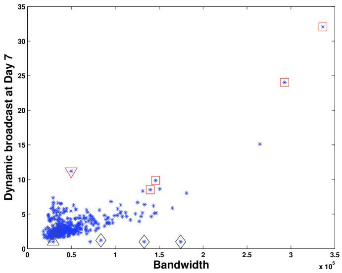
Figure 1: Voice call data, end of Day 6: for each node we show dynamic broadcast measure on vertical axis and bandwidth on horizontal axis. The ringleader is marked with a downward pointing red triangle and the other four inner circle nodes are marked with red squares. After day 6 these individuals are believed to change phone, the ringleader’s subsequent ID is marked with a black upward pointing triangle, and the other inner circle IDs with black diamonds.

We see that the key nodes for day 1 to 6 are much more dominant in terms of dynamic broadcast than overall bandwidth. In particular, the ringleader node has a very modest bandwidth but ranks 8th out of 400 for broadcast communicability.

Figure 2 shows the same information for the data arising from days 7 to 10. We see again that the dynamic broadcast score does a much better job of revealing the inner circle. In particular, the new ID of the ringleader, marked with a black upward pointing triangle, has a very low overall bandwidth but ranks the 5th highest for broadcast centrality. The ‘old’ IDs from the inner circle, marked with red squares, continue to have high bandwidth, but the dynamic broadcast score indicates that they are no longer central players.

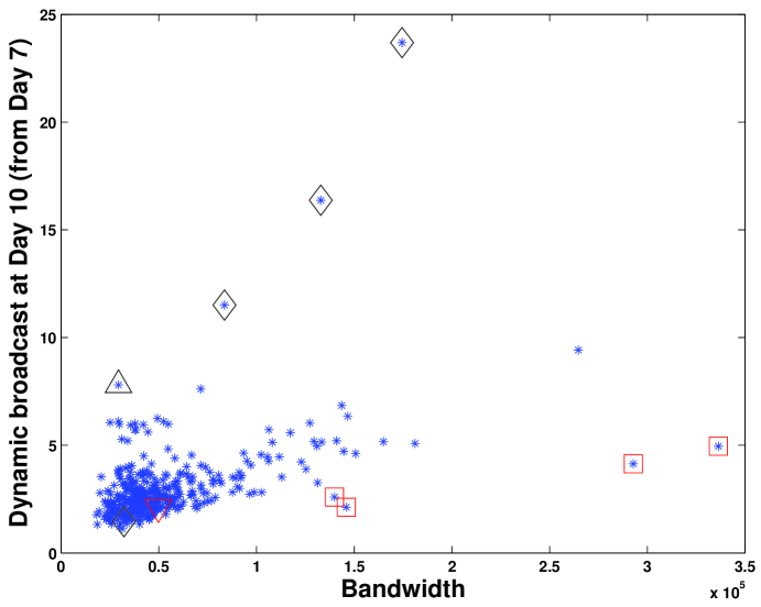
Figure 2: As for Figure 1, using data from day 7 to day 10.

To illustrate point (B), Figure 3 shows the dynamic communicability between the original IDs of the five key players, 200, 1 , 2, 3 and 5, as a function of time. Here, at each time point, we show the average pairwise broadcast plus receive communicability between each pair of nodes in this group scaled by the average pairwise communicability between all pairs of nodes. We see that this running measure is able to track the change in the nature of the network at day 7, when these individuals switch to different IDs.

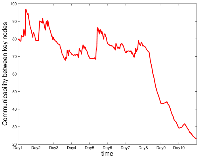
Figure 3: Voice call data: Dynamic communicability between the 5 key nodes (vertical axis) as a function of time (horizontal axis).

In summary, this work has presented what we believe to be the first attempt to pass to the continuum limit in dynamic network centrality. Our framework fits naturally into the context of online or digital recording of human interactions. The ODE setting conveniently avoids the need to discretize the network data into pre-defined snapshots—an approach that can introduce inaccuracies and computational inefficiencies. By defining a continuous time dynamical system, we can simulate with off-the-shelf, state-of-the-art, adaptive numerical ODE solvers, so that time discretization is performed “under the hood”and in a manner that automatically handles considerations of accuracy and efficiency. In particular, in this way, we can deal adaptively with dramatic changes in network behaviour. The ODE framework allows us to downweight information over time, so that a running summary of centrality can be updated in real time without the need to store, or take account of, all previous interaction history. We focused here on the data-driven issue of monitoring node centrality when the time-varying adjacency matrix is available. This has immediate applications to the issue of ranking nodes Blumm et al. (2012), detecting virality Iribarren and Moro (2011) and making time-sensitive strategic decisions Borge-Holthoefer et al. (2013). Further, the ODEs derived here can feed into the development of new network models where the evolution of centrality is coupled to the evolution of topology, and hence they can contribute to modelling, prediction and hypothesis testing.

PG was supported by the Research Councils UK Digital Economy Programme via EPSRC grant EP/G065802/1 The Horizon Digital Economy Hub. DJH acknowledges support from a Royal Society Wolfson Award and a Royal Society/Leverhulme Senior Fellowship.

References

- Holme and Saramäki (2012) P. Holme and J. Saramäki, Physics Reports 519, 97 (2012).
- Barrat et al. (2013) A. Barrat, B. Fernandez, K. K. Lin, and L.-S. Young, Phys. Rev. Lett. 110, 158702 (2013).
- Lambiotte et al. (2011) R. Lambiotte, R. Sinatra, J. C. Delvenne, T. S. Evans, M. Barahona, and V. Latora, Physical Review E 84, 017102+ (2011).
- Stehlé et al. (2011) J. Stehlé, N. Voirin, A. Barrat, C. Cattuto, V. Colizza, L. Isella, C. Regis, J. Pinton, N. Khanafer, W. Van den Broeck, et al., BMC Medicine 9 (2011).
- Grindrod et al. (2011) P. Grindrod, D. J. Higham, M. C. Parsons, and E. Estrada, Physical Review E 83, 046120 (2011).
- Grindrod and Higham (2013) P. Grindrod and D. J. Higham, SIAM Review 55, 118 (2013).
- Tang et al. (2010a) J. Tang, M. Musolesi, C. Mascolo, V. Latora, and V. Nicosia, in SNS ’10: Proceedings of the 3rd Workshop on Social Network Systems (ACM, New York, NY, USA, 2010a), pp. 1–6, ISBN 978-1-4503-0080-3.
- Lentz et al. (2013) H. H. K. Lentz, T. Selhorst, and I. M. Sokolov, Physical Review Letters 110, 118701+ (2013).
- Mucha et al. (2010) P. J. Mucha, T. Richardson, K. Macon, M. A. Porter, and J.-P. Onnela, Science 328, 876 (2010).
- Tang et al. (2010b) J. Tang, S. Scellato, M. Musolesi, C. Mascolo, and V. Latora, Physical Review E 81, 05510 (2010b).
- Gómez et al. (2013) S. Gómez, A. Diaz-Guilera, J. Gómez-Gardeñes, C. J. Pérez-Vicente, Y. Moreno, and A. Arenas, Phys. Rev. Lett. 110, 028701 (2013).
- Dunlavy et al. (2011) D. M. Dunlavy, T. G. Kolda, and E. Acar, ACM Transactions on Knowledge Discovery from Data 5, Article 10, 27 pages (2011).
- Marvel et al. (2011) S. A. Marvel, J. Kleinberg, R. D. Kleinberg, and S. H. Strogatz, Proceedings of the National Academy of Sciences 108, 1771 (2011).
- Traag et al. (2013) V. A. Traag, P. Van Dooren, and P. De Leenheer, PLoS ONE 8, e60063 (2013).
- Grindrod et al. (2012) P. Grindrod, D. J. Higham, and M. C. Parsons, Internet Mathematics 8, 402 (2012).
- Katz (1953) L. Katz, Psychometrika 18, 39 (1953).
- Higham (2008) N. J. Higham, Functions of Matrices: Theory and Computation (Society for Industrial and Applied Mathematics, Philadelphia, PA, USA, 2008), ISBN 978-0-898716-46-7.
- Bilton (2011) N. Bilton, The New York Times September 7 (2011).
- Grinstein et al. (2008) G. G. Grinstein, C. Plaisant, S. J. Laskowski, T. O’Connell, J. Scholtz, and M. A. Whiting, in IEEE VAST (IEEE, 2008), pp. 195–196.
- Blumm et al. (2012) N. Blumm, G. Ghoshal, Z. Forró, M. Schich, G. Bianconi, J. P. Bouchaud, and A. L. Barabási, Physical Review Letters 109, 128701+ (2012).
- Iribarren and Moro (2011) J. L. Iribarren and E. Moro, Physical Review E 84, 046116+ (2011).
- Borge-Holthoefer et al. (2013) J. Borge-Holthoefer, R. A. Baňos, S. Gonzáez-Bailón, and Y. Moreno, Journal of Complex Networks (2013).