A Combinatorial Understanding of Lattice Path Asymptotics

Abstract.

We provide a combinatorial derivation of the exponential growth constant for counting sequences of lattice path models restricted to the quarter plane. The values arise as bounds from analysis of related half planes models. We give explicit formulas, and the bounds are provably tight. The strategy is easily generalized to cones in higher dimensions, and has implications for random generation.

1. Introduction

Lattice path models have enjoyed a sustained popularity in mathematics over the past century, owing in part to their simplicity and ease of analysis, but also their wide applicability both in mathematics, physics, and chemistry. The basic enumerative question is to determine the number of walks of a given length in a given model. The past ten years have seen many interesting developments in the asymptotic and exact enumeration of lattice models, with new techniques coming from computer algebra, complex analysis and algebra. A first approximation to this value is the exponential growth constant, also called the connective constant, which itself carries combinatorial and probabilistic information. For example, it is directly related to the limiting free energy in statistical mechanical models.

A model is defined by the steps that are allowed, and the region to which the walks are restricted (generally cones and strips). Particular focus has been on small step models (where the steps are a subset of $\{0,\pm 1\}^{2}$) restricted to $\mathbb{Z}_{\geq 0}^{2}$, and general approaches versus resolution of individual cases. For example, three distinct strategies for asymptotic enumeration have recently emerged. Fayolle and Raschel [9] have determined expressions for the growth constant for small step models using boundary value problem techniques. Recast as diagonals, techniques of analytic combinatorics of several variables apply to some of the models with D-finite generating functions  [16, 17]. Finally, the important sub-class of excursions, that is, of walks which return to the origin, are well explored via the probability work of Denisov and Wachtel [6, Section 1.5]. Bostan, Raschel and Salvy [4] made their results explicit in the enumeration context. Most of these asymptotic results are obtained with machinery which does not sustain a clear underlying combinatorial picture.

Many of these results exclude singular models: A two dimensional model is singular if the support of the step set is contained in a half plane. Many singular models are either trivial or reduce to a problem in a lower dimension. The singular models are considered in [18, 15].

This paper provides a formula for an upper bound on the growth constant of the counting sequence for lattice models restricted to a convex cone, with intuitive combinatorial interpretations of intermediary computations. Our formula is most explicit in the case of nonsingular 2-dimensional walks restricted to the first quadrant, but is valid for all models. Our general strategy is based on the following basic observation:

In any lattice path model, the set of walks restricted to the first quadrant is a subset of the walks restricted to some half plane which contains that quadrant. Consequently, for any fixed length, the number of walks in that half plane is an upper bound for the number of walks in the quarter plane.

Bounds on walks in half planes are readily computable, for example using the results of Banderier and Flajolet [1]. Remarkably, we are able to give tight bounds on the growth constant by considering all of the half planes that contain the quarter plane. Furthermore, our bounds are insightfully tight in that they give a single simple combinatorial interpretation of the multiple cases treated by Fayolle and Raschel [9]. Our one idea unifies their cases, which depend on various parameters of the model. Furthermore, our approach also applies to singular models. We use only the elementary calculus observation that a minimum of a real valued continuous function $f$ with domain $D$ must occur either at the boundary of $D$ or at a critical point $\tau\in D$ satisfying $f^{\prime}(\tau)=0$. Our approach is combinatorial and readily adaptable to models with larger steps, weighted steps, and to models in higher dimensions. Furthermore, there are implications for random generation, as we discuss in the conclusion.

In an earlier version of this article we conjectured that our bounds were tight. This led to a proof by Garbit and Raschel [12] that the bounds we find in the nonsingular case actually are tight. Simultaneously, and independently, similar results were proved by Duraj [8]. Now, Garbit, Mustafa and Raschel [11] conjecture that in some cases the sub-exponential growth also matches that of the minimizing half-plane, futher validating our interpretation.

1.1. Conventions and notation

Here, a lattice path model is a combinatorial class denoted by $\textsc{R}(\mathcal{S})$ which is defined by a convex cone R, and a finite multiset of allowable steps (vectors), $\mathcal{S}$. We focus on regions that are half-planes through the origin, and the first quadrant $\mathbb{Z}_{\geq 0}^{2}$. We restrict $\mathcal{S}$ to be a finite subset of $\mathbb{Z}^{2}$. A walk of length $n$, say $w=w_{0}w_{1}\dots w_{n}$, is a sequence of points $w_{i}\in\textsc{R}$ such that $w_{i}-w_{i-1}\in\mathcal{S}$ and for $i=1..n$.We denote by $\textsc{R}(\mathcal{S})_{n}$ the subset of all walks of length $n$ in $\textsc{R}(\mathcal{S})$.

The central quantity we investigate is the number of walks with $n$ steps in a given model, $|\textsc{R}(\mathcal{S})_{n}|$. We write $\textsc{H}=\mathbb{R}\times\mathbb{R}_{\geq 0}$ for the upper half plane and $\textsc{Q}=\mathbb{R}_{\geq 0}\times\mathbb{R}_{\geq 0}$ for the first quadrant, and abbreviate $h_{n}=|\textsc{H}(\mathcal{S})_{n}|$ and $q_{n}=|\textsc{Q}(\mathcal{S})_{n}|$ when $\mathcal{S}$ is clear. In this work we focus on models in Q.

A step set is said to be made of small steps if $\mathcal{S}\subseteq\{0,\pm 1\}^{2}\setminus\{(0,0)\}$ and in this case we use the compass abbreviations $NW\equiv(-1,1),N\equiv(0,1),NE\equiv(1,1)$, etc. We might also consider larger regions, and more general step sets. We say a model $\textsc{R}(\mathcal{S})$ is nontrivial if it contains at least one walk of positive length, and if for every boundary of R, there exists an unrestricted walk on $\mathcal{S}$ which crosses that boundary at some point other than an intersection of boundaries (i.e. in two dimensions, not at the origin). The excursions are the sub-class consisting of walks which start and end at the origin. A step set is said to be singular if it is contained within a single half-plane.

The (exponential) growth constant of the sequence is defined as the limit

$$K_{\mathcal{S}}=\lim_{n\rightarrow\infty}q_{n}^{1/n}.$$

The limit exists by a classic argument: $q_{n}\cdot q_{m}\leq q_{n+m}$, so by a Theorem of Hill [13] the limit exists and hence (see [10, Theorem IV.7]) it must be the reciprocal of the dominant singularity of the generating function of the $q_{n}$. The present work determines bounds for the growth constant, $K_{\mathcal{S}}$, of the sequence $\{q_{n}\}$.

Our strategy uses the simple relation that if $\textsc{Q}\subset\textsc{R}$, then $\textsc{Q}(\mathcal{S})_{n}\subset\textsc{R}(\mathcal{S})_{n}$ and hence $q_{n}\leq|\textsc{R}(\mathcal{S})_{n}|$. This is true for all $n$, hence it is also true that $\lim_{n}q_{n}^{1/n}\leq\lim_{n}|\textsc{R}(\mathcal{S})_{n}|^{1/n}$. It turns out, by considering well chosen regions, we are able to perfectly bound the growth constant $K_{\mathcal{S}}$. Our preferred bounding regions are the half planes

$$\textsc{H}_{\theta}=\{(x,y):x\sin\theta+y\cos\theta\geq 0\}$$

where $\theta\in[0,\pi/2]$. We denote by $K_{\mathcal{S}}(\theta)$ the growth constant of the sequence of the number of walks of length $n$ in this region:

$$K_{\mathcal{S}}(\theta)=\lim_{n\rightarrow\infty}|\textsc{H}_{\theta}(\mathcal{S})_{n}|^{1/n}.$$

Using the relation

$$K_{\mathcal{S}}\leq K_{\mathcal{S}}(\theta)\quad\text{for all }0\leq\theta\leq\pi/2,$$

we can deduce bounds on $K_{\mathcal{S}}$, by finding explicit expressions for $K_{\mathcal{S}}(\theta)$.

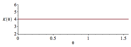
(a)

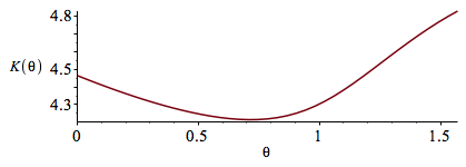
(b)

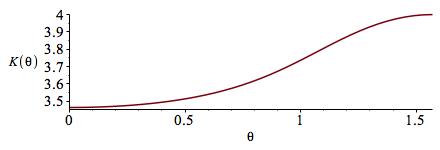
(c)

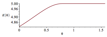
(d)

Figure 1. Graphs of $K_{\mathcal{S}}(\theta)$ for various $\mathcal{S}$

Figure 1 illustrates this concept by considering several models, and their exponential growth in several regions.

1.2. The main result and the plan of the paper

Our main result, Theorem 9, is an explicitly computable bound on $K_{\mathcal{S}}$, and its combinatorial interpretation. It is determined by minimizing $K_{\mathcal{S}}(\theta)$ as a function of $\theta$. In several cases it is easily seen to be tight, by comparing to the well-understood subclass of excursions.

We start at Lemma 7, where we adapt the formulas of Banderier and Flajolet to give a formula for $K_{\mathcal{S}}(\theta)$, for given $\mathcal{S}$ and $\theta$. We then show that $K_{\mathcal{S}}(\theta)$ defines a continuous function in $\theta$. Since each $\textsc{H}_{\theta}$ contains Q, $K_{\mathcal{S}}(\theta)$ is an upper bound on $K_{\mathcal{S}}$ for any $\theta$ satisfying $0\leq\theta\leq\pi/2$. Finally, we determine the location of the minimum upper bound in Theorem 9 by basic calculus techniques, since $K_{\mathcal{S}}(\theta)$ is an explicit function of $\theta$.

In Section 4, we show that these results give precisely the values found by Fayolle and Raschel for the nonsingular models, demonstrating the bounds are tight. It is Theorem 16 which vindicates the description of this work as a combinatorial interpretation of the formulas provided by Fayolle and Raschel.

Our strategy applies to more general classes of models, for example, multiple steps in the same direction, longer steps, and higher dimensional models. The quantities we recover in these cases are, transparently, upper bounds and they can be compared against experimental data as a check for tightness. This led us to conjecture that our approach gives tight upper bounds more generally and hence actually finds the growth constants, which has subsequently been proven for some particular cases in [12, Corollary 10] through probabilistic arguments.

2. Walks in a half plane

Models restricted to a half plane are well understood, and we recall here some basic results. The set $\textsc{H}(\mathcal{S})$ of walks restricted to the upper half plane with steps from the finite multiset $\mathcal{S}$ is in bijection with unidimensional walks with steps from the multiset $\mathcal{A}=\{j:(i,j)\in\mathcal{S}\}$ because horizontal movement does not lead to any interaction with the boundary of H. We thus consider half plane models as unidimensional models defined by sets of real numbers. We retain the same notation: $\textsc{H}(\mathcal{A})_{n}=\{w_{0}w_{1}\dots w_{n}:w_{i}\geq 0,w_{i}-w_{i-1}\in\mathcal{A}\}$. The multiset $\mathcal{A}$ is said to be nontrivial, if it contains at least one positive and one negative value. There are two ways for a multiset $\mathcal{A}$ to be trivial in a half plane: either $\mathcal{A}$ contains only non-negative elements and we call it unrestricted; or $\mathcal{A}$ contains only non-positive elements. Unless otherwise stated, we assume that the models are nontrivial. It is worth noting that Theorem 1 still holds in the unrestricted case.

The key ingredients for the enumeration are as follows. The drift of $\mathcal{A}$ is the sum $\delta(\mathcal{A})=\sum_{a\in\mathcal{A}}a$ and the inventory of $\mathcal{A}$ is $A(u)=\sum_{a\in\mathcal{A}}u^{a}$; notice that these are related by $\delta(\mathcal{A})=A^{\prime}(1)$.

Theorem 1 (Modified from Theorem 4 of Banderier and Flajolet [1]).

Let $\mathcal{A}$ be a multiset of integers which defines a nontrivial unidimensional walk model. Let $A(u)=\sum_{a\in\mathcal{A}}u^{a}$. The number $h_{n}$ of walks of length $n$ in $\textsc{H}(\mathcal{A})$ depends the inventory on the sign of the drift $\delta(\mathcal{A})=A^{\prime}(1)$ as follows:

$$h_{n}\sim\begin{cases}\nu_{0}\,A(1)^{n}&\text{if }\delta(\mathcal{A})>0\\ \nu_{1}\,A(1)^{n}\,n^{-1/2}&\text{if }\delta(\mathcal{A})=0\\ \nu_{2}\,A(\tau)^{n}\,n^{-3/2}&\text{if }\delta(\mathcal{A})<0\\ \end{cases}.$$

Here $\tau$ is the unique positive critical point of $A(u)$ and $\nu_{0},\nu_{1}$ and $\nu_{2}$ are explicit, real constants.

Proof.

This follows directly from [1]. Remark the case of unrestricted sets of steps $\mathcal{A}$, $h_{n}=|\mathcal{A}|^{n}=A(1)^{n}$ so setting $\nu_{2}=1$ gives the result. ∎

Banderier and Flajolet prove these formulas by applying transfer theorems to explicit generating functions, which they first derive. The strategy requires integer steps however: The models with real-valued steps are not necessarily representable by context-free grammars, and the generating functions are not necessarily algebraic. However, results on the growth constant appear in the probability literature [7]. It is rather straightforward to deduce from the integer case by a limit argument which we present next.

Theorem 2.

Let $\mathcal{A}$ be a multiset of real numbers which defines a nontrivial unidimensional walk model. Let $A(u)=\sum_{a\in\mathcal{A}}u^{a}$. The number $K_{\mathcal{A}}=\lim_{n\rightarrow\infty}h_{n}^{1/n}$, where $h_{n}$ is of walks of length $n$ in $\textsc{H}(\mathcal{A})$, depends the inventory on the sign of the drift $\delta(\mathcal{A})=A^{\prime}(1)$ as follows:

(2.1) $$K_{\mathcal{A}}=\begin{cases}|\mathcal{A}|&\text{if }\delta(\mathcal{A})\geq 0\\ A(\tau)&\text{otherwise}.\end{cases}$$

Here $\tau$ is the unique positive critical point of $A(u)$.

First, remark that in the unrestricted case, as $h_{n}=|\mathcal{A}|^{n}$, and the drift is non-negative, hence the theorem is also true under weaker hypotheses including this case.

Theorem 1 establishes this formula for $\mathcal{A}\subset\mathbb{Z}$. The proof for other real nontrivial models $\mathcal{A}\subset\mathbb{R}$ is established from the integer base case in three steps:

1. We show that if Equation (2.1) holds for the multiset $\mathcal{A}$, then it is also true for the multiset $r\mathcal{A}=\{ra:a\in\mathcal{A}\}$ when $r>0$ in Lemma 3;

2. We then deduce that the formula holds for multisets of rationals in Remark 4;

3. Finally, we prove that the formula holds for multisets of reals by proving that a limiting construction of rational models gives the result. This is done in Section 2.3.

We remark that the growth constant of the sequence counting the number of excursions of length $n$ in H (in the integer case) can be shown to be $A(\tau)$ using a strategy similar to the proof of Theorem 1 [1, Theorem 3]. This does not translate as smoothly in the real valued case, as this formula does not adequately capture when the class is empty.

2.1. Some facts about the inventory $A(u)$

The first two steps of the proof of Theorem 2 follow from basic behaviour of $A(u)$.

Lemma 3 (Scaling Lemma).

Let $\mathcal{A}$ be a finite multiset of real numbers which is either unrestricted or nontrivial and let $A(u)=\sum_{a\in\mathcal{A}}u^{a}$. Suppose further that Equation (2.1) holds for $K_{\mathcal{A}}$. For any $r>0$, define $\mathcal{B}=r\mathcal{A}=\{ra:a\in\mathcal{A}\}$. Then the growth constant $K_{\mathcal{B}}$ of the sequence $b_{n}=|\textsc{H}(\mathcal{B})_{n}|$ satisfies

$$K_{\mathcal{B}}=\begin{cases}|\mathcal{B}|&\text{if }\delta(\mathcal{B})\geq 0\\ B(\tau_{\mathcal{B}})&\text{otherwise}\end{cases}.$$

Here $B(u)=\sum_{b\in\mathcal{B}}u^{b}$ and $\tau_{\mathcal{B}}$ is the unique positive critical point of $B(u)$.

Proof.

The lattice model $\textsc{H}(\mathcal{B})$ is combinatorially isomorphicto $\textsc{H}(\mathcal{A})$, so their growth constants are the same. The formula follows because their drifts have the same sign, and since $B(u)=A(u^{r})$ and $\tau_{\mathcal{B}}=\tau_{\mathcal{A}}^{1/r}$, thus $B(\tau_{\mathcal{B}})=A(\tau_{\mathcal{A}})$. ∎

Remark 4.

For any finite multiset of rational numbers $\mathcal{B}$, there is an $r>0$, for example, the least common multiple of the denominators in $\mathcal{B}$, so that $\mathcal{A}=r\mathcal{B}$ is a set of integers. By Theorem 1, $K_{\mathcal{A}}$ satisfies Equation (2.1). Consequently, by Lemma 3, since $\mathcal{B}=\frac{1}{r}\mathcal{A}$, it is also true that $K_{\mathcal{B}}$ satisfies Equation (2.1).

Lemma 5 ($A(u)$ is strictly convex at its minimum).

Given a finite multiset $\mathcal{A}$ of real numbers which defines a nontrivial unidimensional model, the real valued function $A(u)=\sum_{a\in\mathcal{A}}u^{a}$ has a unique positive critical point $\tau$. The function is minimized at this point, and is strictly convex on a neighbourhood of $\tau$. Furthermore, if $\delta(\mathcal{A})=0$, then the unique critical point occurs at $u=1$.

Proof.

If there are no elements in the range $(0,1)$ then the result holds term by term. Otherwise it is possible to scale so that all elements are in that range.

∎

2.2. The continuity of $A(\tau_{\mathcal{A}})$ as a function of $\mathcal{A}$

To prove Theorem 2, we consider the function $A(u)$, evaluated at its critical point. In particular we view this as a function of the step lengths. In the following lemma, $\ell$ represents the number of elements in the step set.

Lemma 6.

Let $F:\mathbb{R}^{\ell}\times\mathbb{R}_{>0}\rightarrow\mathbb{R}$ be the function defined by

$$F((x_{1},x_{2},\dots,x_{\ell}),u)=F(\mathbf{x},u)=\sum_{j=1}^{\ell}u^{x_{j}}.$$

Furthermore, let $\mathbf{a}\in\mathbb{R}^{\ell}$ have at least one positive component and one negative component, and denote by $\tau(\mathbf{a})$ the unique positive critical point of the map $u\mapsto F(\mathbf{a},u)$. There is a neighbourhood $\mathcal{U}$ of $\mathbf{a}$ such that the function

$$\kappa(\mathbf{x})=F(\mathbf{x},\tau(\mathbf{x})),$$

is continuous in $\mathbf{x}$ on $\mathcal{U}$.

Proof.

The results is a consequence of the implicit function theorem applied to $f(\mathbf{x},u)=\frac{\partial F(\mathbf{x},u)}{\partial u}$ around the point $\mathbf{a}$. ∎

2.3. Proof of Theorem 2 in the case of real multisets

Proof of Theorem 2.

Let $\mathcal{A}\subset\mathbb{R}$ be a finite multiset of real numbers which is either unrestricted or nontrivial. To prove that $K_{\mathcal{A}}$ satisfies Equation (2.1) we build two sequences of rational step sets which converge to $\mathcal{A}$. We then squeeze the growth constant $K_{\mathcal{A}}$ of $h_{n}=|\textsc{H}(\mathcal{A})_{n}|$ into the desired form.

For each $a\in\mathcal{A}$, let $\{a_{i}^{+}\}$ and $\{a_{i}^{-}\}$ be rational sequences satisfying

$$0\leq a_{i}^{+}-a\leq\frac{1}{2^{i}}\qquad\mbox{and}\qquad 0\leq a-a_{i}^{-}\leq\frac{1}{2^{i}}.$$

We define two multisets

$$\mathcal{A}_{i}^{+}=\{a_{i}^{+}:a\in\mathcal{A}\}\qquad\mbox{and}\qquad\mathcal{A}_{i}^{-}=\{a_{i}^{-}:a\in\mathcal{A}\}.$$

The drift is additive, thus for each $i$,

$$\delta(\mathcal{A}_{i}^{-})=\sum_{a\in\mathcal{A}}a_{i}^{-}\leq\sum_{a\in\mathcal{A}}a\leq\sum_{a\in\mathcal{A}}a_{i}^{+}=\delta(\mathcal{A}_{i}^{+}).$$

Note that Remark 4 applies to both $\mathcal{A}_{i}^{-}$, and $\mathcal{A}_{i}^{+}$ because both are multisets of rational numbers and hence (2.1) is valid for the growth constants, $K_{\mathcal{A}_{i}^{-}}$ and $K_{\mathcal{A}_{i}^{+}}$ respectively.

Furthermore, starting from a half-plane walk and making some steps slightly more positive can never talk the walk outside the half-plane so, by the construction of $\mathcal{A}_{i}^{+}$ and $\mathcal{A}_{i}^{-}$ we get a natural injection

$$\textsc{H}(\mathcal{A}_{i}^{-})\xhookrightarrow{\textsc{H}}(\mathcal{A})\xhookrightarrow{\textsc{H}}(\mathcal{A}_{i}^{+})$$

and hence

(2.2) $$K_{\mathcal{A}_{i}^{-}}\leq K_{\mathcal{A}}\leq K_{\mathcal{A}_{i}^{+}}.$$

We claim

$$\lim_{i\rightarrow\infty}K_{\mathcal{A}_{i}^{-}}=K_{\mathcal{A}}=\lim_{i\rightarrow\infty}K_{\mathcal{A}_{i}^{+}},$$

and $K_{\mathcal{A}}$ is given by the formula of Theorem 1. To prove this claim observe the following. In the negative drift case Lemma 6 guarantees that the $\lim_{i\rightarrow\infty}K_{\mathcal{A}_{i}^{\pm}}$ converge and, from Lemma 5, when $\delta(\mathcal{A})=0$, $\tau_{\mathcal{A}}=1$ so a negative drift $\mathcal{A}_{i}^{-}$ limits correctly up to a $0$ drift $\mathcal{A}$. In all cases $\mathcal{A}_{i}^{\pm}\rightarrow\mathcal{A}$ so $\delta(\mathcal{A}_{i}^{\pm})\rightarrow\delta(\mathcal{A})$. Therefore by Remark 4

$$\lim_{i\rightarrow\infty}K_{\mathcal{A}_{i}^{\pm}}=\begin{cases}|\mathcal{A}|&\text{if }\delta(\mathcal{A})\geq 0\\ A(\tau_{\mathcal{A}})&\text{otherwise}\end{cases}$$

so the squeeze theorem gives the result. ∎

2.4. Other half planes

Next, we extend to other half planes, each defined by an angle: $\textsc{H}_{\theta}=\{(x,y):x\sin\theta+y\cos\theta\geq 0\}$. Note that for $\theta\in[0,\pi/2)$ this region is equal to $\{(x,y):y\geq-mx\}$ where $m=\tan\theta$. The upper half plane is given by $\textsc{H}_{0}$ and the right half plane is $\textsc{H}_{\pi/2}$. In this latter case, we use the extended reals, and write $m=\infty$. The enumeration of lattice paths in $\textsc{H}_{\theta}$ emulates the enumeration of lattice paths in H.

(a) The step set $\mathcal{S}=\{N,E,SW\}$ (in blue), and its projection onto the line $y=x/2$ (in purple, dashed)

(b) Step set for the unidimensional model $H(\{1,2,-3\})$

Figure 2. Three representations for models of walks with steps from $\mathcal{S}=\{N,E,SW\}$ restricted to the region $\{y\geq-2x\}$, defined by $\theta=\arctan(2)$: (A) $H_{\theta}(\mathcal{S})$, and its unidimensional projection and (B) $H(\{1,2,3\})$, a scaling of $\mathcal{A}(\theta)$.

 

Lemma 7.

Let $\mathcal{S}\subset\mathbb{Z}^{2}$ be a finite multiset and let $\textsc{H}_{\theta}=\{(x,y):x\sin\theta+y\cos\theta\geq 0\}$ and let $\mathcal{A}(\theta)=\{i\sin\theta+j\cos\theta:(i,j)\in\mathcal{S}\}$. The combinatorial class $\textsc{H}_{\theta}(\mathcal{S})$ is combinatorially isomorphic to $\textsc{H}(\mathcal{A}(\theta))$.

Furthermore, if $\mathcal{S}$ is a nontrivial or unrestricted step set for $\textsc{H}_{\theta}$ then the growth constant $K_{\mathcal{S}}(\theta)$ for the sequence $|\textsc{H}_{\theta}(\mathcal{S})_{n}|$ is the value $K_{\mathcal{A}(\theta)}$ determined by Theorem 2.

Proof.

Here it suffices to consider the displacement of each step in the step set in the direction orthogonal to the boundary. See Figure 2 for an example. The steps $(0,1)$ and $(1,0)$ respectively have displacement $\cos\theta$ and $\sin\theta$ in this direction, the other steps follow by linearity. This gives rise to a unidimensional half plane model with step set $\mathcal{A}(\theta)$ to which Theorem 2 applies if $\mathcal{A}(\theta)$ is nontrivial or unrestricted, which occurs precisely when $\mathcal{S}$ is nontrivial or unrestricted in $\textsc{H}_{\theta}$. ∎

Example 8 ($\mathcal{S}=\{N,E,SW\}$= ).

For any $\theta\in[0,\pi/2]$, $\textsc{Q}(\mathcal{S})\subseteq\textsc{H}_{\theta}(\mathcal{S})$ and the following classes are combinatorially isomorphic

$$\textsc{H}_{\theta}(\mathcal{S})\cong\textsc{H}(\{\cos\theta,\sin\theta,-\cos\theta-\sin\theta\}).$$

When $\theta\neq\pi/2$, we can scale the model by $\cos\theta^{-1}$. Let $m=\tan\theta,\theta\neq\pi/2$, then $\textsc{H}_{\theta}(\mathcal{S})\cong\textsc{H}(\{1,m,-m-1\})$. For $\theta=\pi/2$, remark $\textsc{H}_{\pi/2}(\mathcal{S})\cong\textsc{H}(\{1,0,-1\})$.

3. Bounds for lattice path models in the quarter plane

As we have already noted in the introduction, the exact enumeration of quarter plane models has been well explored recently. In the case of small steps, Bousquet-Mélou and Mishna identified 79 non-isomorphic, nontrivial small step models [5]. The associated generating functions are known to be D-finite for 23 of these models. After algebraic, the D-finite models are easiest to enumerate asymptotically, and several approaches for this have been successful [3, 16, 17, 2].

The non-D-finite models have been more elusive. Fayolle and Raschel have determined expressions for the growth constant for 74 models [9]. We summarize their formulas in Section 4. Melczer and Mishna determined formulas for the the remaining five models [15], and also for highly symmetric models of arbitrary dimension [16].

To describe these formulas we again need the drift of the model, denoted $\delta(\mathcal{S}):$

$$\delta(\mathcal{S})=\sum_{s\in\mathcal{S}}s=(\delta_{x},\delta_{y}).$$

Here we use a shorthand for classifying drift profiles. For each component, we note if the drift is positive $(+)$, zero $(0)$ or negative $(-)$. For example, if $\delta(\mathcal{S})\in\mathbb{R}_{>0}\times\mathbb{R}_{\geq 0}$, the drift profile is $(+,+/0)$.

The inventory of the model is the Laurent polynomial $S(x,y)$ defined

$$S(x,y)=\sum_{(i,j)\in\mathcal{S}}x^{i}y^{j}.$$

This is the two dimensional analog to $A$, and it can be used to express some useful quantities

$$S(1,1)=|\mathcal{S}|\qquad\delta_{x}=\left.\frac{\partial}{\partial x}S(x,1)\right|_{x=1}=P_{x}(1,1),\qquad\delta_{y}=\left.\frac{\partial}{\partial y}S(1,y)\right|_{y=1}=P_{y}(1,1).$$

The unidimensional case analysis depended upon the existence of a positive critical point of the inventory. Its existence was a consequence of the non-triviality of the model. The two dimensional case is similar.

We use the result that in the case of a nontrivial, non singular model there is a unique solution $(\alpha,\beta)\in\mathbb{R}^{2}_{>0}$ to the equation $P_{x}(x,y)=P_{y}(x,y)$ when $\mathcal{S}$ is nonsingular. This is a straightforward consequence of equation manipulation. We call this point the critical point of the inventory. It is straightforward to show that there is no such $(\alpha,\beta)$ with $\alpha$ and $\beta$ positive when $\mathcal{S}$ is singular.

3.1. Bounds from half-plane models

An upper bound on the growth constant of a quarter plane model can always be determined by appealing to a half plane model using the same steps restricted to lie in a region containing the first quadrant. In this section we describe how to determine the half plane which gives the best bound. The main result is Theorem 9. It is followed by examples of its application, its proof, and then in Section 4 a proof that, in the case of small steps, the bound is the same as the exact formula of Fayolle and Raschel. In some cases, this is easy to see, as the upper bound is the same as the lower bound given by excursions.

Theorem 9 (Main Theorem).

Let $\mathcal{S}\subset\mathbb{Z}^{2}$ be a finite multiset that defines a nontrivial quarter plane model $\textsc{Q}(\mathcal{S})$. Then,

1. the growth constant $K_{\mathcal{S}}=\lim_{n\rightarrow\infty}q_{n}^{1/n}$ satisfies

   $$K_{\mathcal{S}}\leq K_{\mathcal{S}}(\theta)\quad\text{ for all }\quad 0\leq\theta\leq\pi/2,$$

   where $K_{\mathcal{S}}(\theta)$ is the growth constant for the associated rotated half plane model, as defined in Lemma 7;

2. the function $K_{\mathcal{S}}(\theta)$ is continuous as a function of $\theta$.

If $\mathcal{S}$ is non-singular, with inventory $S(x,y)$, then denote by $(\alpha,\beta)$ the unique solution in $\mathbb{R}^{2}_{>0}$ to

$$P_{x}(\alpha,\beta)=P_{y}(\alpha,\beta)=0.$$

If $\beta\neq 1$ and $\ln\alpha/\ln\beta\geq 0$, then let $\theta^{*}=\arctan\frac{\ln\alpha}{\ln\beta}$. If $\delta_{x}\sin\theta^{*}+\delta_{y}\cos\theta^{*}\leq 0$ then the minimum value of $K_{\mathcal{S}}(\theta)$ is attained at $\theta^{*}$, and

$$K_{\mathcal{S}}(\theta^{*})=S(\alpha,\beta).$$

Otherwise, if any of these conditions are not satisfied, or if $\mathcal{S}$ is singular, the minimum is attained at one of the endpoints of the range: either $0$ or $\pi/2$.

Note that the minimum being obtained as described does not preclude it also being attained elsewhere. Notably, $K_{\mathcal{S}}(\theta)$ is constant in the range $0\leq\theta\leq\pi/2$ when the drift profile is non-negative in each component. We also note that the drift condition $\delta_{x}\sin\theta^{*}+\delta_{y}\cos\theta^{*}\leq 0$ only comes into play for the mixed drift profiles $(+,-)$ and $(-,+)$. The basic idea is that $K_{\mathcal{S}}(\theta)$ gets truncated at $|\mathcal{S}|$ but otherwise its critical point behavious comes from that of $S(x,y)$ in the manner detailed below. So the minimum of $K_{\mathcal{S}}(\theta)$ comes either from $S(\alpha,\beta)$, from an endpoint, or from the constant truncated part, which then must also be achieved at an endpoint.

Before we prove this result, we consider three examples to develop some intuition on the behaviour. Recall that to each pair of quarter plane model $\mathcal{S}$, and angle $\theta$, we associate the unidimensional step set $\mathcal{A}(\theta)=\{i\sin\theta+j\cos\theta:(i,j)\in\mathcal{S}\}$. We define the following shorthand for its inventory and critical point:

$$A_{\theta}\equiv\sum{a\in_{\mathcal{A}(\theta)}}u^{a}\quad\text{and}\quad\tau_{\theta}\equiv\tau_{\mathcal{A}(\theta)}.$$

Example 10 ($\mathcal{S}=\leavevmode\hbox to9.16pt{\vbox to9.25pt{\text{[drawing]}}}$).

This is an example of a nontrivial, singular model. There is no point $(\alpha,\beta)$ as in the theorem statement. The drift profile is $(+,+)$, and hence $K_{\mathcal{S}}(\theta)$ is constant in the domain. We deduce $K_{\mathcal{S}}\leq K_{\mathcal{S}}(\theta)=|S|=4$. This value is tight, according to the formulas of Melczer and Mishna [15].

Example 11 ($\mathcal{S}=\leavevmode\hbox to9.16pt{\vbox to9.34pt{\text{[drawing]}}}$).

This is not a singular model, and the inventory $S(x,y)=y+\frac{1}{y}+\frac{x}{y}+\frac{1}{xy}$ has a unique critical point at $(1,\sqrt{3})$. The optimal angle given by Theorem 9 is

$$\theta^{*}=\arctan(\ln(1)/\ln(\sqrt{3}))=0.$$

Now, $\textsc{Q}(\mathcal{S})\subset\textsc{H}(\mathcal{S})$, and $\textsc{H}(\mathcal{S})\cong\textsc{H}(\mathcal{A}(0))\cong\textsc{H}(\{1,-1,-1,-1\})$. This leads to the bound $K_{\mathcal{S}}\leq K_{\mathcal{S}}(0)=A_{0}(\sqrt{3})=S(1,\sqrt{3})=2\sqrt{3}$. This is tight in comparison to the formula given for $K_{\mathcal{S}}$ by Fayolle and Raschel [9]. We shall see that this is a special case of Lemma 15.

Example 12 ($\mathcal{S}=\leavevmode\hbox to9.25pt{\vbox to9.34pt{\text{[drawing]}}}$).

We can numerically compute the critical point $(\alpha,\beta)$ of the inventory $S(x,y)=y+\frac{x}{y}+\frac{1}{y}+\frac{1}{xy}+\frac{1}{x}$ as $(\alpha,\beta)\approx(1.6760,1.8091)$. Consequently, the minimising angle is $\theta^{*}\approx 0.2281\pi\approx\arctan(0.8712)$. The best bound is computed $K_{\mathcal{S}}(\theta^{*})\approx 4.2148$. The exact value of the critical point is a tight bound. Note that the minimising half plane is not defined by the line perpendicular to the drift. The drift vector is $\delta(\mathcal{S})=(-1,-2)$, so the perpendicular has slope $-1/2$. We contrast this with slope given by the bound, at $-0.8712$.

Example 12 demonstrates that the best half plane is not defined by the perpendicular to the drift vector (a common hypothesis). Rather, the slope is connected to the Cramér transformation in probability [6]. Denisov and Wachtel assign the probability $p_{ij}=\frac{\alpha^{i}\beta^{j}}{S(\alpha,\beta)}$ to the step $(i,j)$ so that the drift of the weighted steps, given by $\sum_{(i,j)\in\mathcal{S}}p_{ij}$, is $(0,0)$, and then apply tools for walks with no drift. It is clear here, perhaps, why their methods apply only to nonsingular walks – they require the existence of $\alpha$ and $\beta$. Bostan, Raschel and Salvy in [4] also discuss the combinatorics of this transform, and show that  $S(\alpha,\beta)$ is the growth constant for excursions in the quarter plane, which is a subclass of walks, hence $S(\alpha,\beta)$ is a lower bound for the growth constant. We offer the interpretation of $S(\alpha,\beta)$ as the exponential growth of walks restricted to the half plane $H_{\theta}$ for the angle $\theta=\arctan(\frac{\ln\alpha}{\ln\beta})$ (or the right half plane when $\beta=1$).

3.2. The function $K_{\mathcal{S}}(\theta)$

The function $K_{\mathcal{S}}(\theta)$ is surprisingly simple, for fixed $\mathcal{S}$. In the case of half-plane walks, the growth constant for the counting sequence for the walks with arbitrary endpoint is either the number of steps, or given by the growth constant for excursions. The deciding factor is the drift.

In our model of changing half planes, the drift is given by the following smooth function of $\theta$:

$$\sum_{(i,j)\in\mathcal{S}}(i\sin\theta+j\cos\theta)=\delta_{x}\sin\theta+\delta_{y}\cos\theta.$$

Thus, $K_{\mathcal{S}}(\theta)$ is either the number of steps, or given by $A_{\theta}(\tau_{\theta})$, and switches between them when the drift is 0. Several different possibilities are presented in Figure 1. Roughly, the function $A_{\theta}(\tau_{\theta})$ is $\pi$-periodic and attains a single maximum given by the number of steps, and a single minimum. If that minimum is in the interval $[0,\pi/2]$ it is also the minimum of $K_{\mathcal{S}}(\theta)$.

These functions are well behaved, and we can accurately predict the point where $K_{\mathcal{S}}(\theta)$ attains a minimum. First, we establish the continuity of $K_{\mathcal{S}}(\theta)$ in the next lemma, and then we determine the complete set of critical points, and whether or not they are maxima, or minima, in Lemma 14.

Lemma 13.

Suppose $\mathcal{S}\subset\mathbb{Z}^{2}$ defines a nontrivial quarter plane model. Then $K_{\mathcal{S}}(\theta)$ defines a continuous function on the domain $\theta\in[0,\pi/2]$.

Proof.

The value of $K_{\mathcal{S}}(\theta)$ is defined piecewise according to the value of $\delta(\mathcal{A}(\theta))=\sum_{(i,j)\in\mathcal{S}}(i\sin\theta+j\cos\theta)=\delta_{x}\sin\theta+\delta_{y}\cos\theta$:

$$K_{\mathcal{S}}(\theta)=\begin{cases}|\mathcal{S}|&\text{if }\delta(\mathcal{A}(\theta))\geq 0\\ A_{\theta}(\tau_{\theta})&\text{otherwise}.\end{cases}$$

The function $A_{\theta}(\tau_{\theta})$ is continuous as a consequence of Lemma 6 since $A_{\theta}(\tau_{\theta})=\kappa(x(\mathcal{S},\theta))$ where

$$\kappa(\mathbf{x})=\sum_{j=1}^{\ell}\tau(\mathbf{x})^{x_{j}}.$$

The condition $\delta(\mathcal{A}(\theta))\geq 0$ defines an interval in $[0,\pi/2]$; consequently $K_{\mathcal{S}}(\theta)$ is piecewise continuous. Finally, as $\delta(\mathcal{A}(\theta))$ approaches $0$, $K_{\mathcal{S}}(\theta)$ tends to $|\mathcal{S}|$, by Lemma 5 the function is continuous at points where $\delta(\mathcal{A}(\theta))=0$.

∎

Next we pinpoint the location of the minima.

Lemma 14.

Let $\mathcal{S}\subseteq\mathbb{Z}^{2}$ be the step set of a nontrivial quarterplane model. When they exist let $(\alpha,\beta)$ be the positive critical point of $S(x,y)$ and $\theta^{\prime}$ be $\arctan(\ln\alpha/\ln\beta)$. If they exist and $\delta(\mathcal{A}(\theta^{\prime}))\leq 0$ then $K_{\mathcal{S}}(\theta)$ achieves its minimum value at $\theta^{\prime}$. Otherwise $K_{\mathcal{S}}(\theta)$ achieves its minimum value at an end point.

Specifically, the minimum value of $K_{\mathcal{S}}(\theta)$ is achieved at $\theta^{*}$, determined as follows

1. if $\delta(\mathcal{S})=(0/+,0/+)$, then for all $\theta^{*}\in[0,\pi/2]$, $K_{\mathcal{S}}(\theta^{*})=|S|$;

2. if $\mathcal{S}$ is singular then, $\theta^{*}\in\{0,\pi/2\}$;

3. if $\mathcal{S}$ is nonsingular then the inventory $S(x,y)$ has a unique critical point $(\alpha,\beta)\in\mathbb{R}_{\geq 0}^{2}$. If $\beta=1$ then $\theta^{*}=\pi/2$. If not, set $\theta^{\prime}=\arctan(\ln\alpha/\ln\beta)$. If $\delta(\mathcal{A}(\theta^{\prime}))\geq 0$, then $\theta^{*}\in\{\pi/2,0\}$. Otherwise, $\theta^{*}=\theta^{\prime}$. In this final case, the growth constant coincides with that of excursions, that is, $K_{\mathcal{S}}(\theta^{*})=S(\alpha,\beta)$.

Proof.

The function is decided by the evolution of the drift. If the drift profile is $(+/0,+/0)$, then $K_{\mathcal{S}}(\theta)=|S|$. Otherwise, the curve takes the value of $A_{\theta}(\tau_{\theta})$ for some sub-interval, and it is in this interval where the minimum occurs.

It turns out that it is easier to work with the value that determines the slope, $m=-\tan(\theta)$. To this end we define $\overline{\mathcal{A}}(m)=\{im+j:(i,j)\in\mathcal{S}\}$, and $\overline{\mathcal{A}}(\infty)=\{i:(i,j)\in\mathcal{S}\}$. Remark that $\overline{\mathcal{A}}(m)$ is a scaled version of $\mathcal{A}(\theta)$, scaled by $\cos\theta^{-1}$. Thus, the two unidimensional models are are combinatorially isomorphic and so the exponential growth of the two models are the same. We find the minimizing slope, $m^{*}$.

Consider $G(u,m)=\sum_{(i,j)\in\mathcal{S}}u^{im+j}$, the inventory of $\overline{A}(m)$. Now, $K_{\mathcal{S}}(\theta)=G(u_{m}^{*},m)$ where $u_{m}^{*}>0$ satisfies $G_{u}(u_{m}^{*},m)=0$. We minimize $G(u_{m^{*}},m)$ as a function of $m\geq 0$ by solving for $(u,m)$ satisfying $G_{m}(u,m)=0$ and $G_{u}(u,m)=0$. We apply the chain rule, by first remarking $G(u,m)=S(u^{m},u)$:

(3.1) $$G_{m}(u,m) = \left.u^{m}\ln uP_{x}(x,y)\right|_{\begin{subarray}{c}x=u^{m}\quad\\ y=u\end{subarray}}$$

(3.2) $$G_{u}(u,m) = \left.mu^{m-1}P_{x}(x,y)\right|_{\begin{subarray}{c}x=u^{m}\quad\\ y=u\end{subarray}}+\left.P_{y}(x,y)\right|_{\begin{subarray}{c}x=u^{m}\quad\\ y=u\end{subarray}}.$$

There is a solution when $u=1$ and $G_{u}(u,m)=0$. This is precisely the case when $-\delta_{x}/\delta_{y}=m$, since $P_{x}(1,1)=\delta_{x}$ and $P_{y}(1,1)=\delta_{y}$. In Lemma 13 we have shown this to be a maximum value, since $G(1,m)=|\mathcal{S}|$, the largest possible value, at this point.

The only other possible solution is when $P_{y}(x,y)=P_{x}(x,y)=0$ itself has positive solution $(\alpha,\beta)$. Thus either the minimum of $K_{\mathcal{S}}(\theta)$ comes from such an $(\alpha,\beta)$ or it is at an end point. It remains only to determine when each occurs.

If $\mathcal{S}$ is singular, no appropriate $(\alpha,\beta)$ exists so the minimum of $A_{\theta}(\tau_{\theta})$, and hence $K_{\mathcal{S}}(\theta)$, occurs at a boundary.

If $\mathcal{S}$ is nonsingular, there is a unique positive $(\alpha,\beta)$. If $\beta=1$, the minimum occurs when $\theta=\pi/2$, so assume that $\beta\neq 1$. Then $(u^{*},m^{*})=(\beta,\ln\alpha/\ln\beta)$ is a critical point of $G(u,m)$ in the desired domain. Now, it is possible that when this point occurs, in fact, the half-plane model defined by $\theta$ is in a positive drift regime. In this case the minimum of $K_{\mathcal{S}}(\theta)$ is at a boundary. Assume otherwise that the half-plane models near the critical point have negative drift.

In this cse, $A_{\theta}(\tau_{\theta})$ has a minimum at the angle $\theta^{*}$ corresponding to $m^{*}$. For any fixed $m$ near $m^{*}$, the function $G(u,m)$ is convex as a function of $u$. For fixed $m$ near $m^{*}$, the minimum of $G(u,m)$ as a function of $u$ is, by definition, $A_{\theta}(\tau_{\theta})$ for the angle corresponding to $m$. Consequently in a sufficiently small neighbourhood of $(u^{*},m^{*})$, $G(u,m)$ is convex both in $u$ and in $m$, so $G(u,m)$ is convex as a two variable function at $(u^{*},m^{*})$. Therefore this $(u^{*},m^{*})$ is a minimum.

Therefore when the half-plane drift at the critical point is negative, the minimum of both $A_{\theta}(\tau_{\theta})$ and $K_{\mathcal{S}}(\theta)$ occurs at $\theta^{*}$. In this case, we compute the growth factor by evaluating at the critical point. That is,

$$K_{\mathcal{S}}(\theta^{*})=G(u^{*},m^{*})=S((u^{*})^{m^{*}},u^{*})=S(\alpha,\beta).$$

∎

Now, we put these ideas together.

Proof of Theorem 9.

Since $\mathcal{S}$ is a nontrivial model, then $A_{\theta}$ is either a nontrivial or an unrestricted model for all $\theta\in[0,\pi/2]$. For any $\theta\in[0,\pi/2]$, $q_{n}\leq|\textsc{H}{(\mathcal{A}(\theta))}_{n}|$ for any $n$, and thus the growth constants of the sequence satisfy $K_{\mathcal{S}}\leq K_{\mathcal{S}}(\theta)$. The latter is minimized at the stated $\theta^{*}$ by Lemma 14. ∎

4. The case of small steps: a different approach

4.1. The work of Fayolle and Raschel

Fayolle and Raschel [9, Remark 4.9] describe the location of the dominant singularity in the generating function for nonsingular small step quarter plane models. Their formula depends on the drift $\delta(\mathcal{S})=(\delta_{x},\delta_{y})$, along with another parameter of the model called the covariance. We do not use this parameter, except to compare to their formulas. The covariance of a step set, denoted $\gamma(\mathcal{S})$ is defined as

$$\gamma(\mathcal{S})=\left.\frac{\partial^{2}}{\partial x\partial y}S(x,y)\right|_{(x,y)=(1,1)}-\delta_{x}\delta_{y}.$$

In the case of small steps the inventory always has the form

$$S(x,y)=a(x)y+b(x)+c(x)y^{-1}=\tilde{a}(y)x+\tilde{b}(y)+\tilde{c}(y)x^{-1}.$$

They prove that there are four possible values for $K_{\mathcal{S}}$:

(4.1) $$\begin{gathered}|\mathcal{S}|,\qquad\rho_{0}^{-1}\equiv S(\alpha,\beta)\\ \rho_{Y}^{-1}\equiv{b(1)+2\sqrt{a(1)c(1)}},\qquad\rho_{X}^{-1}\equiv{\tilde{b}(1)+2\sqrt{\tilde{a}(1)\tilde{c}(1)}}.\end{gathered}$$

As before, $(\alpha,\beta)$ is the unique positive solution in $\mathbb{R}_{>0}^{2}$ satisfying

$$P_{x}(\alpha,\beta)=0\qquad P_{y}(\alpha,\beta)=0.$$

Furthermore, in their Remark 4.9 they determine conditions on the sign of  $\delta(\mathcal{S})$ and $\gamma$ which decide which of the four values is correct for a given nonsingular model.

These results have some natural interpretations. If $\delta(\mathcal{S})$ is non-negative in both components then the growth constant is as for unrestricted walks. If $\delta(\mathcal{S})$ is positive in the first component, and negative in the second, then growth constant is the same as the walks that remain in the upper half plane. The value $S(\alpha,\beta)$ is the growth constant for excursions [6, 4]. If $\delta(\mathcal{S})$ is negative in both components then the growth constant is the same as the growth constant for excursions in the region. This mirrors the behaviour in the case of unidimensional walks. The specific formulas they obtain are simply the result of their cases picking out when $K_{\mathcal{S}}(\theta)$ is minimized at an end point or the critial point. In this way, we are able unify the six cases, and deliver a single interpretation of the formulas.

Specifically, the next lemma shows how the values $\rho_{0},\rho_{X},\rho_{Y},1/|\mathcal{S}|$ arise as $K_{\mathcal{S}}(\theta)$, for various $\theta$.

Lemma 15.

For any nontrivial quarter plane model $\textsc{Q}(\mathcal{S})$ with $\mathcal{S}\subset\{0,\pm 1\}^{2}$, the following equalities hold:

$$\rho_{Y}^{-1}=A_{0}(\tau_{0})\qquad\rho_{X}^{-1}=A_{\pi/2}(\tau_{\pi/2}).$$

Proof.

This is proved by simply unraveling the notation:

$$A_{0}(u)=\sum_{(i,j)\in\mathcal{S}}u^{j}=S(1,u)$$

$$\text{and so}\quad A_{0}^{\prime}(u)=[u]S(1,u)-\frac{1}{u^{2}}[u^{-1}]S(1,u)\implies\tau_{0}=\sqrt{\frac{[u^{-1}]S(1,u)}{[u]S(1,u)}}.$$

Consequently,

$$A_{0}(\tau_{0})=[y^{0}]S(1,y)+2\sqrt{[y]S(1,y)\cdot[y^{-1}]S(1,y)}=\rho_{Y}^{-1},$$

which is precisely the formula for $\rho_{Y}^{-1}$ given in Equation 4.1. The $\rho_{X}$ case is similar since $A_{\pi/2}(u)=\sum_{(i,j)\in\mathcal{S}}u^{i}$. ∎

We conclude this section with a discussion that the bounds are tight, i.e.

$$K_{\mathcal{S}}=\min_{\theta\in[0,\pi/2]}K_{\mathcal{S}}(\theta)$$

for all small step quarter plane models. Recall that subsequent to the first version of this document being circulated, this has been proved by Garbit and Raschel, but we can understand it combinatorially.

$(\delta_{x},\delta_{y})$	$\gamma$	$\alpha$	$\beta$	$\ln(\alpha)/\ln(\beta)$	$\tan(\theta^{*})$	$K_{\mathcal{S}}$
$(+,+)$		$<1$	$<1$	$+$	$\frac{\ln\alpha}{\ln\beta}$	$|\mathcal{S}|$
$(+,0)$
$(0,+)$
$(0,0)$		$1$	$1$		1	$S(\alpha,\beta)=|\mathcal{S}|$
$(0,-)$	$-$	$>1$	$>1$	$+$	$\frac{\ln\alpha}{\ln\beta}$	$S(\alpha,\beta)$
	$0$	$1$		$0$	$0$	$S(\alpha,\beta)=\rho_{Y}^{-1}$
	$+$	$<1$		$-$	$0$	$\rho_{Y}^{-1}$
$(+,-)$		$<1$		$-$	$0$
$(-,0)$	$-$	$>1$	$>1$	$+$	$\frac{\ln\alpha}{\ln\beta}$	$S(\alpha,\beta)$
	$0$		$1$	$\infty$	$\infty$	$S(\alpha,\beta)=\rho_{X}^{-1}$
	$-$		$<1$	$-$	$\infty$	$\rho_{X}^{-1}$
$(-,+)$			$>1$	$-$	$\infty$
$(-,-)$		$>1$	$>1$	+	$\frac{\ln\alpha}{\ln\beta}$	$S(\alpha,\beta)$

Table 1. The value of $K_{\mathcal{S}}$ for nonsingular nontrivial quarter plane models defined by a finite, step set $\mathcal{S}\subset\{\pm 1,0\}^{2}$. This value can be computed either using sign information about the drift $\delta$ and the covariance $\gamma$, or from information about $\alpha$ and $\beta$.

Theorem 16.

Let $\mathcal{S}\subseteq\{0,\pm 1\}^{2}$ be a finite set defining a nontrivial, nonsingular quarter-plane lattice path model. The growth constant $K_{\mathcal{S}}$ for the number $q_{n}$ of walks of length $n$ in $\textsc{Q}(\mathcal{S})$ satisfies

(4.2) $$K_{\mathcal{S}}=\min_{\theta\in[0,\pi/2]}K_{\mathcal{S}}(\theta).$$

The location of the minimum is summarized in Table 1.

To prove Theorem 16, we could directly relate the drift profile to the value of $\min_{\theta\in[0,\pi/2]}K_{\mathcal{S}}(\theta)$, and show that this matches the values obtained by Fayolle and Raschel.

The different cases are summarized in Table 1. It is possible to prove the results in Table 1 by considering the two equations/inequalities that arise from drift profiles and follow the implications in a straightforward way to deduce the sign of both $\ln\alpha$ and $\ln\beta$. Some general case reductions can simplify some of the work. As the inequality manipulations are rather tedious, we do not include them here. It is also possible to simply test the 79 small step cases in order to verify the result.

5. Extensions and applications

Our half plane bounding strategy does not rely on the size of the steps nor the convex cone in which the paths are restricted. Naive numerical calculations on examples of quarter plane walks with larger steps and of three dimensional models, so far tested in the non-negative octant, suggest the bounds remain tight.

Furthermore, in a recent study of three dimensional walks [BoBoKaMe15], Bostan, Bousquet-Mélou, Kauers, and Melczer guessed differential equations satisfied by the generating functions of some small step models, and using this they were able to conjecture the exact growth constants. We verified that, in each of the cases for which they had data, the growth constant for the model $O(\mathcal{S})$, where $O=\mathbb{R}_{\geq 0}^{3}$, is equal to the minimal bound.

These observations led us to the following conjecture.

Conjecture 1.

Let $\mathcal{S}\subset\mathbb{Z}^{d}$ be a finite multiset of steps. Let $K_{\mathcal{S}}$ be the growth constant for the enumerative sequence counting the number of walks restricted to the first orthant. Let $\mathcal{P}$ be the set of hyperplanes through the origin in $\mathbb{R}^{d}$ which do not meet the interior of the first orthant. Given $p\in\mathcal{P}$ let $K_{\mathcal{S}}(p)$ be the growth constant of the walks on $\mathcal{S}$ which are restricted to the side of $p$ which includes the first orthant. Then

$$K_{\mathcal{S}}=\min_{p\in\mathcal{P}}K_{\mathcal{S}}(p).$$

Note that in all dimensions, $K_{\mathcal{S}}(p)$ can be computed by projecting the steps onto the normal to $p$, and enumerating the resulting unidimensional model. Thus, if true, our conjecture would give an elementary way to understand and compute the growth constant of any class of first orthant restricted walks.

The work of Garbit and Raschel translates this into a probabilistic context, and in particular they have proved for it in Corollary 9 of [12] under the conditions on models which essentially avoid singular, and trivial models.

Our half plane interpretation has important implications for random generation. A naive rejection strategy to generate quarter plane walks might first generate walks in the whole plane, and reject them as they leave the quarter plane. Models with a $(-,-)$ drift profile perform rather poorly in this scheme. However, when the exponential growth rate of a class of quarter plane walks is the same as some class of half plane walks which contain it, the following rejection scheme is provably efficient. The half plane walks with rational slope form an algebraic language, and are easily generated. Rejecting walks from this class when they leave the quarter-plane is remarkably efficient. There are additional details required when the slope is not rational, and the theory is developed by Lumbroso, Mishna and Ponty [14].

Approximations such as we compute here can aid other direct strategies. For example, the strategy of diagonals used by Melczer, Mishna and Wilson relies on determining a set of critical points to set up the intergral computations. Having a tight bound on the exponential growth in hand is useful in this process, as soem candidates can be eliminated immediately.

6. Acknowledgments

We are grateful to Andrew Rechnitzer for some initial discussions on using the upper half plane as an upper bound, in addition to useful comments from Kilian Raschel, Michael Renardy, Philippe Biane, and Jean-François Marckert and Jérémie Lumbroso. MM is also very grateful to LaBRI, Université de Bordeaux, which acted as a host institution during the completion of this work.

References

• [1] C. Banderier and Ph. Flajolet. Basic analytic combinatorics of directed lattice paths. Theoret. Comput. Sci., 281(1-2):37–80, 2002. Selected papers in honour of Maurice Nivat.
• [2] A. Bostan, F. Chyzak, M. van Hoeij, M. Kauers, and L. Pech. Hypergeometric expressions for generating functions of walks with small steps in the quarter plane. pages 1–30, 2016. http://arxiv.org/abs/1606.02982.
• [3] A. Bostan and M. Kauers. Automatic classification of restricted lattice walks. In DMTCS Proceedings of the 21st International Conference on Formal Power Series and Algebraic Combinatorics (FPSAC’09), Hagenberg, Austria, pages 203–217, 2009.
• [4] A. Bostan, K. Raschel, and B. Salvy. Non-D-finite excursions in the quarter plane. J. Combin. Theory Ser. A, 121:45–63, 2014.
• [5] M. Bousquet-Mélou and M. Mishna. Walks with small steps in the quarter plane. In Algorithmic probability and combinatorics, volume 520 of Contemp. Math., pages 1–39. Amer. Math. Soc., Providence, RI, 2010.
• [6] D. Denisov and V. Wachtel. Random walks in cones. Ann. Probab., 43(3):992–1044, 2015.
• [7] R. A. Doney. On the asymptotic behaviour of first passage times for transient random walk. Probab. Theory Related Fields, 81(2):239–246, 1989.
• [8] J. Duraj. Random walks in cones: the case of nonzero drift. Stochastic Process. Appl., 124(4):1503–1518, 2014.
• [9] G. Fayolle and K. Raschel. Some exact asymptotics in the counting of walks in the quarter plane. In 23rd Intern. Meeting on Probabilistic, Combinatorial, and Asymptotic Methods for the Analysis of Algorithms (AofA’12), Discrete Math. Theor. Comput. Sci. Proc., AQ, pages 109–124. Assoc. Discrete Math. Theor. Comput. Sci., Nancy, 2012.
• [10] Ph. Flajolet and R. Sedgewick. Analytic combinatorics. Cambridge University Press, Cambridge, 2009.
• [11] R. Garbit, S. Mustapha, and K. Raschel. Random walks with drift in cones. In preparation, 2016.
• [12] R. Garbit and K. Raschel. On the exit time from a cone for random walks with drift. Rev. Mat. Iberoamericana, 32(2):511–532, 2016.
• [13] E. Hille. Functional Analysis and Semi-Groups. American Mathematical Society Colloquium Publications, vol. 31. American Mathematical Society, New York, 1948.
• [14] J. Lumbroso, M. Mishna, and Y. Ponty. Taming reluctant random walks in the positive quadrant. In Jean-Marc Fédou, editor, Proceedings of International conference on random generation of combinatorial structures GASCom’16, Electronic Notes in Discrete Mathematics. Elsevier, 2016. To appear.
• [15] S. Melczer and M. Mishna. Singularity analysis via the iterated kernel method. Combin. Probab. Comput., 23(5):861–888, 2014.
• [16] S. Melczer and M. Mishna. Asymptotic lattice path enumeration using diagonals. Algorithmica, 75:782–811, 2016.
• [17] S. Melczer and M. Wilson. Asymptotics of lattice walks via analytic combinatorics in several variables. In Proceedings of FPSAC’16, Discrete Math. Theor. Comput. Sci. Proc., 2016.
• [18] M. Mishna and A. Rechnitzer. Two non-holonomic lattice walks in the quarter plane. Theoret. Comput. Sci., 410(38-40):3616–3630, 2009.