Scaling of hysteresis loop of interacting polymers under a periodic force

Abstract

Using Langevin Dynamics simulations, we study a simple model of interacting-polymer under a periodic force. The force-extension curve strongly depends on the magnitude of the amplitude $(F)$ and the frequency ($\nu$) of the applied force. In low frequency limit, the system retraces the thermodynamic path. At higher frequencies, response time is greater than the external time scale for change of force, which restrict the biomolecule to explore a smaller region of phase space that results in hysteresis of different shapes and sizes. We show the existence of dynamical transition, where area of hysteresis loop approaches to a large value from nearly zero area with decreasing frequency. The area of hysteresis loop is found to scale as $F^{\alpha}\nu^{\beta}$ for the fixed length. These exponents are found to be the same as of the mean field values for a time dependent hysteretic response to periodic force in case of the isotropic spin.

I introduction

Many cellular processes are driven by mechanical forces. Synthesis and degradation of proteins shtilerman ; huang  , transcription and replication of nucleic acids, and packing of DNA in a capsid are few examples neuwald ; cook ; Guo . In fact, biological motors fueled by ATP transform chemical energy to mechanical energy through the hydrolysis process albert ; tom . Periodic consumption of ATP to ADP suggests that biological motors generate forces of periodic nature. For examples, DNA-B, a ring like hexameric helicase that pushes through the DNA like a wedge dnab . Williams and Jankowsy nphii showed that viral RNA helicase NPH-II that hops cyclically from the double stranded (ds) to the single stranded (ss) part of DNA and back during the ATP hydrolysis cycle. It is also proposed that pulling force resulting from ATP consumption is used by proteasomes and mitochondrial to unfold proteins wang ; Lee ; Navon .

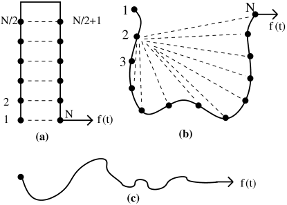
Figure 1: Schematic representations of an interacting polymer: (a) DNA in the zipped state, (b) a self-interacting polymer chain and (c) extended form of an interacting polymer under the influence of applied force ($f$). In all these cases, one end of polymer is fixed and the other end may be subjected to a constant force or periodic stretching force. For DNA, the dotted lines represent base pairing interaction among complimentary nucleotides (say 1 to $N/2$ are made up of adenine (A) and $(N/2+1)$ to $N$ are made up of complimentary nucleotides i.e. thymine (T)). In this case, base pairing interaction is restricted in such a way that the first monomer forms base pair with the $N^{th}$ monomer and $2^{nd}$ monomer forms base pair with $(N-1)^{th}$ and so on. For a self-interacting polymer, the dotted lines show the attractive interaction among non-bonded monomers. In this case, any monomer of a chain can interact with the rest of monomers of the chain. Here, for example, we have shown the second monomer of the chain, which is interacting with rest of non-bonded monomers. Similarly, other monomers interact with rest of the non-bonded monomers.

In recent years, there are theoretical efforts to understand the response of periodic force on the bio-molecules Vidybida ; Braun ; Pereverzev ; Lomholt ; Lin . Most of these studies were confined to understand the kinetics under the equilibrium conditions kumarphys . However, living systems are the open systems and never at equilibrium. In the equilibrium, bio-molecule follows the force in phase. The force-extension curve for a periodic force, keeping other intensive quantities fixed, would result in retracing thermodynamic path, ending at the initial state. In contrast, in the non-equilibrium situation, the difference between the relaxation time and the external time scale for change of force would restrict the bio-molecule to explore a smaller region of the phase space, thereby creates hysteresis i.e. a difference in the response to an increasing and decreasing force. Hysteresis is well studied in the context of the spin systems madan1 ; madan2 ; dd ; bkc . It was found that the area of the hysteresis loop scales as $h^{\alpha}\nu^{\beta}$, where $h$ and $\nu$ are the amplitude and the frequency of the applied magnetic field, respectively. The values of $\alpha$ and $\beta$ differ from system to system bkc and the reason for it has been discussed in siam .

Though, hysteresis has been observed in single molecule experiments Liphardt ; Collin ; Schlierf ; Hatch ; Li1 ; Born ; Friddle ; Diezemann , however, many aspects of these phenomena are yet to be explored. In a recent work Kapri , Kapri showed that using the work theorem sadhu , it is possible to extract the equilibrium force-extension curve from the hysteresis loops. In another work, a dynamical transition has been proposed, where the area of loop changes with the frequency of the applied force from nearly zero to a finite value, similar to the one seen in case of spin systems arxiv ; arxiv1 . In low frequency limit, for a short DNA (16 base pairs), the scaling exponents ($\alpha$ and $\beta$) are found to be the same as of the isotropic spin system. This raises many questions such as does the dynamical transition exist in the thermodynamic limit? Do these exponents depend on the length of the DNA? What is the role of molecular interaction (involved in the stability of bio-molecules) on the dynamical transition. In this context, it is pertinent to mention here that in Ref. arxiv1 , modeling of DNA involves a single polymer chain with native interaction (base pairing) as shown in Fig. 1a. Will scaling exponents change, for a self-interacting polymer (SIP) chain, where a monomer of the chain can interact (non-native interaction) with the rest (Fig. 1b) of monomers of the chain kumar_prl ? The present paper addresses some of such issues. In section II, we develop a simple model of polymer and impose certain constraints to model different bio-polymers. We briefly describe in this section the Langevin Dynamics(LD) simulations Allen ; Smith to obtain the thermodynamic observables. In Sec. III, we study equilibrium properties of a short DNA and a SIP and obtain the force-extension curves and the force-temperature diagrams. Section IV deals with the dynamical transition associated with DNA of different lengths. We obtain the various exponents associated with the hysteresis loop. We also discuss dynamical transition associated with a SIP and obtain the scaling exponents. In Sec. V, we discuss finite size scaling. Sec. VI describes the dynamics near $T=0$, which helped us in identifying natural frequency to describe the transition. Finally in Sec. VII, we summarize our results and discuss the future perspectives.

II Model and Method

Bio-molecules exhibit a wide range of time scales over which specific processes take place kumarphys . For example, local motion, which involves atomic fluctuation, side chain motion and loop motion, occurs in the length scale of 0.01 to 5 Å and the time involved in such a process is of the order of $10^{-15}$ to $10^{-12}$s. The motion of helix and protein domain belong to the rigid body motion, whose typical length scales are in between 1 to 100 Å and time involved in such motion is in between $10^{-9}$ to $10^{-6}$s. Here, our interest is in the large-scale motion e.g. helix-coil transition, folding-unfolding transition of proteins and coil-globule transition in polymer, which occurs in the length scale more than 5 Å and time involved is about $10^{-7}$ to $100$ s. Since, such a time scale is not amenable computationally, therefore, we consider a coarse-grained model of a linear polymer chain and impose restrictive interaction among monomers in such a way that it captures some essential properties of different bio-polymers Li ; Kouza ; MSLi_BJ07 ; thiru ; mishra . We follow Ref. arxiv , where the energy of the model system is defined by the following expression:

$$E=\sum_{i=1}^{N-1}k(d_{i,i+1}-d_{0})^{2}+\sum_{i=1}^{N-2}\sum_{j>i+1}^{N}(\frac{B}{d_{i,j}^{12}}-C(\frac{A_{i,j}}{d_{i,j}^{6}})),$$ (1)

where, $N$ is the total number of beads/monomers present in the polymer chain. The distance between $i^{th}$ and $j^{th}$ bead is denoted by $d_{i,j}$ $=$ $|\vec{r}_{i}-\vec{r}_{j}|$, where $\vec{r}_{i}$ and $\vec{r}_{j}$ are the position of bead $i$ and $j$, respectively. First term of Eq. 1 is the potential function for covalent bonds between two consecutive monomers and is represented by the harmonic potential with spring constant $k(=100)$ mishra . Second term in the expression represents Lennard-Jones (L-J) potential, which models non-bonded interaction among monomers of the chain. The first term of L-J potential takes care of the excluded volume effect i.e. two monomers can not occupy the same space. Second term of the L-J potential gives the attractive interaction between all monomers except the adjacent one. The parameter $d_{0}(=1.12)$ corresponds to the equilibrium distance in the harmonic potential, which is close to the equilibrium position of the average L-J potential. The values of $A_{ij}$ and $B$ are set to be equal to 1. The parameter $C=1.0$ is chosen here for the DNA. For the SIP, we choose $d_{0}=1.00$, $k=16.67$ and $C=2.0$, respectively as adopted in the model discussed in the Ref. mickal .

In force induced transitions, one stretches a bio-polymer from its ground state (native conformation), therefore, properties associated with this transition are mainly governed by its native topology. The Go Model, which is based on the native-topology is found to be quite useful in studying the influence of mechanical forces on the bio-polymers go ; Poland ; Navin . It may be noted that by restricting $A_{ij}$ (second term of L-J potential), it is possible to model native topology of different bio-polymers. For example, if half of a polymer chain is allowed to interact with the other half of a chain, in such a way that the first monomer interacts only with the $N^{th}$ monomer (last one), and the second monomer interacts with the $(N-1)^{th}$ and so, the ground state conformation resembles a zipped conformation of DNA of $N_{p}$ ($=N/2$) base pairs as shown in Fig. 1a arxiv ; arxiv1 ; mishra ; Foster . Similarly, if any monomer of the chain is allowed to interact with the rest of non-bonded monomers of the polymer chain, the ground state will resemble the globule (collapsed) state of a self-interacting polymer kumar_prl . The native topology-based model, turns out to be quite helpful in predicting the mechanism involved in the DNA unzipping and protein unfolding. It also allowed to decipher the free-energy landscapes of bio-polymersLi ; Kouza ; MSLi_BJ07 ; thiru ; mishra ; pablo .

The dynamics of the system is obtained from the Langevin equation Allen ; Smith ; MSLi_BJ07 . It is a stochastic differential equation, which introduces friction and noise terms in to Newton’s second law to approximate the effects of temperature and environment:

$$m\frac{d^{2}{\bf r}}{dt^{2}}=-{\zeta}\frac{d{\bf r}}{dt}+{\bf F_{c}}+\Gamma,$$ (2)

where $m(=1)$ and $\zeta(=0.4$) are the mass of a bead and the friction coefficient, respectively. Here, ${\bf F_{c}}$ is defined as $-\frac{dE}{d{\bf r}}$ and the random force $\Gamma$ is a white noise Smith , and is related to the friction coefficient by fluctuation dissipation theorem i.e., $<{\Gamma(t)\Gamma(t^{\prime})}>=2\zeta T\delta(t-t^{\prime})$. It may be noted that the friction term used here only influences the kinetics, not the thermodynamic properties Li ; Kouza . The choice of this dynamics keeps temperature ($T$) constant throughout the simulation. The equation of motion is integrated by using the $6^{th}$ order predictor-corrector algorithm with time step $\delta t$=0.025 Smith for DNA and $\delta t$=0.005 for the SIP, respectively. The results are averaged over many trajectories.

III Equilibrium properties of bio-polymers

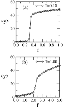
Figure 2: (a) Equilibrium force-extension ($f-y$)
curve for DNA and (b) for a self-interacting polymer.

The equilibrium properties of DNA unzipping has been studied in the constant force ensemble (CFE) for the fixed length mishra . Here, we also study the equilibrium properties of self-interacting polymer in CFE and compare its result with DNA. The equilibrium has been checked by calculating the auto-correlation function box ; berg for the square of the end-to-end distance and the number of contacts mishra . Moreover, these results are tested over many seeds and the stability of data against at least ten times longer run. We have used $2\times 10^{9}$ time steps out of which first $5\times 10^{8}$ steps are not taken in the averaging. In the equilibrium condition, we add an energy $-\vec{f}.\vec{y}$ to the total energy of the system given by Eq. 1 mishra . We calculate the average extension $<y>$ (distance between the end monomers) at different values of $f$. The force-extension curves (Fig. 2) for both cases show qualitatively similar behavior. Below the critical force, the systems remain in the zipped (or globule) state, and above it, in the unzipped (or coil) state. It may be noted that, if we decrease the force keeping the other intensive parameters fixed, the system nearly retraces the path showing that it is in the equilibrium.

The equilibrium force-temperature ($f-T$) diagram may be obtained by monitoring the energy fluctuation (or the specific heat) with temperature at different forces $f$ Li ; Kouza ; mishra . The peak in the specific heat curve gives the melting temperature at that $f$, which is consistent with the $f-y$ curve for that temperature $T$. The phase boundary in the $f-T$ diagrams (Fig. 3) separates the region, where the DNA (or SIP) exists in a zipped (or globule) state from the region, where it exists in the unzipped (or coil) state. It is evident from these plots (Fig. 3) that the melting temperature decreases with the applied force in accordance with the earlier studies bhat99 ; marenprl . We find that the peak height increases with the chain length, though, the transition temperature (melting temperature) remains almost the same for different lengths.

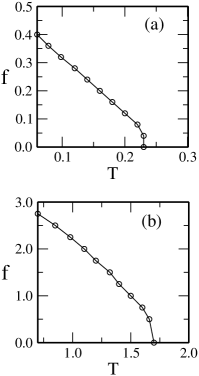
Figure 3: (a) Equilibrium force-temperature ($f-T$) diagram of DNA and (b) for a self-interacting polymer.

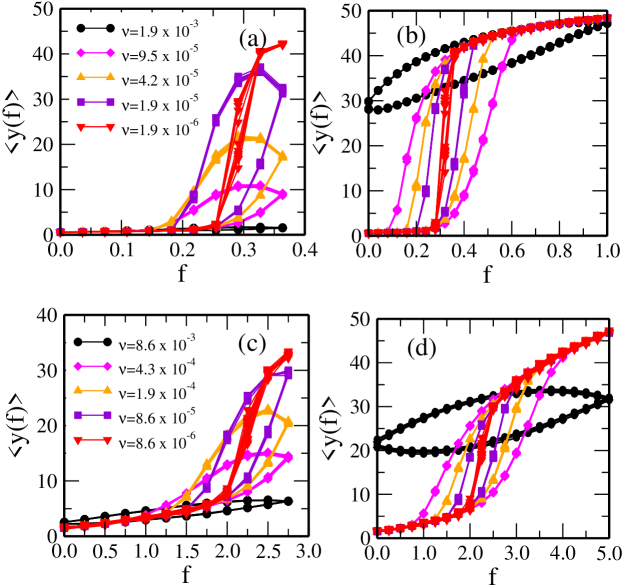
Figure 4: The averaged extension of DNA as a function of cyclic force of amplitude (a) 0.4 and (b) 1.0 at different $\nu$. Figs. (c) and (d) are for the SIP for low (2.75) and high amplitude (5.0), respectively. It is evident from these plots (Figs. a & c) that at low amplitude and high frequency, the system remains in the zipped (collapsed) state, whereas at high amplitude and high frequency (Figs. b & d), the system remains in the extended state with a small hysteresis loop. As $\nu$ decreases, both the systems extend to the hysteretic state with a bigger loop. For $\nu\rightarrow 0$, the hysteresis loop vanishes and the system approaches its equilibrium path irrespective of the magnitude of amplitudes of the applied force.

IV Dynamical transition at finite temperature

In order to study the dynamical stability of the bio-molecule under a periodic force arxiv , we add an energy $-f(t).y(t)$ to the total energy of the system given by Eq. 1. The value of $f$ increases to its maximum value $F$ in $m_{s}$ steps at interval $\Delta f(=0.01)$ and then decreases to $0$ in the same way arxiv ; arxiv1 . Since, we are interested in the non-equilibrium regime, we allow only $n$ LD time steps (much below the equilibrium time) in each increment of $\Delta f$. Here, $y(t)$ is the distance between the two ends of the chain at that instant of time. We keep sum of the time spent $\tau(=2nm_{s})$ in each force cycle constant to keep $\nu(=1/\tau)$ constant. Hence, for a given $F$, $n$ controls the frequency. By varying $F$ (keeping $\nu$ fixed) or $\nu$ (keeping $F$ fixed), it is possible to induce a dynamical transition between a time averaged zipped (globule) state or unzipped (coil) state to a hysteretic state (oscillating between the zipped and the unzipped state).

The average extension of the DNA (Fig. 4 a & b) and SIP (Fig. 4 c & d) clearly exhibits hysteresis under the periodic force. We have performed average over 1000 cycles for different initial conformations. In Figs,(4a-d) we have shown the plots for 10 different initial conformations. All these curves overlap indicating that the system is in the steady state, irrespective of the starting conformation (zipped or unzipped). If the time averaged $y(f)$ is less than $5$, we call the system is in the zipped state, where as if $y(f)>5$, it is in the open state or in the unzipped state arxiv ; arxiv1 . At low amplitude, the chain remains in the zipped state (Fig. 4a), with almost negligible loop area. As the frequency decreases, the system explores more phase space and acquires conformations belonging to the unzipped state. We calculate the dynamical order parameter bkc i.e. the area of the hysteresis loop, which is defined as

$$A_{loop}=\oint y(f).df.$$ (3)

One may notice from Fig. 4 that the area of loop increases as the frequency decreases. After a certain frequency, the area of the loop starts decreasing, and the system nearly retraces the equilibrium path at low frequency. The self-interacting polymer, which shows the existence of globule state (Fig. 2) at low $T$, exhibits the similar behavior (Fig. 4 c & d). However, at high amplitude, where the dsDNA shows the existence of the stretched state for all frequencies, SIP shows the existence of two states i.e. extended and stretched. Since, for the SIP the ground state energy is quite large compare to DNA, the unfolding force is also found to be larger than the dsDNA. It is in accordance with the experiments kumarphys . The other interesting observation from these plots is that though $f$ decreases from its maximum value F to 0 (Fig. 4 a & c), $y(f)$ increases and there is some lag, after which it decreases. One may recall that the relaxation time is much higher compare to the time spent at each interval of $\Delta f$, and therefore, an increase in $y(f)$ with decreasing $f$, indicates that the system gets more time to relax. As a result $y(f)$ approaches a path, which is close to the equilibrium. Once the system gets enough time, the lag disappears. A similar lag can be seen, when the system starts from the open state at high $\nu$. However, in this case as $\nu$ decreases, $y(f)$ decreases with increasing $f$. In both the cases , whether DNA starts from the zipped or open state, as $\nu\rightarrow 0$, the system approaches the equilibrium $f-y$ curve and the area of loop vanishes.

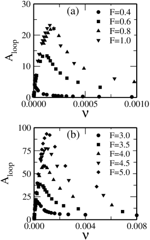
Figure 5: Figures show the variation of area of hysteresis loop with the frequency at different force amplitudes (a) for DNA and (b) for SIP. For both cases, the area of loop increases to its maximum with the frequency and then again approaches to zero. In these cases, the system approaches the equilibrium from the non-equilibrium as the frequency decreases.

In Fig. 5, we have plotted the area of hysteresis loop of DNA (Fig. 5a) and SIP (Fig. 5b) with the frequency at different force amplitudes. One can see from these plots that the area of hysteresis loop increases with decrease in the frequency and starts decreasing after a certain frequency. At a very low frequency, the system approaches its equilibrium i.e. the extension nearly retraces its path under the cyclic force. Fig. 6 a & b shows the variation of loop area for DNA and SIP, respectively, with force amplitude at different frequencies. Here, the area also increases with the amplitude and after certain amplitude, it starts decreasing similar to Fig. 5 . In this case, however, the system goes far away from the equilibrium.

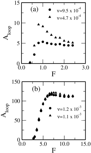
Figure 6: Variation of the area of hysteresis loop with force amplitude at different frequencies: (a) for DNA and (b) SIP. In this case, the system never approaches to equilibrium and always remains far away from the equilibrium as the amplitude of force increases.

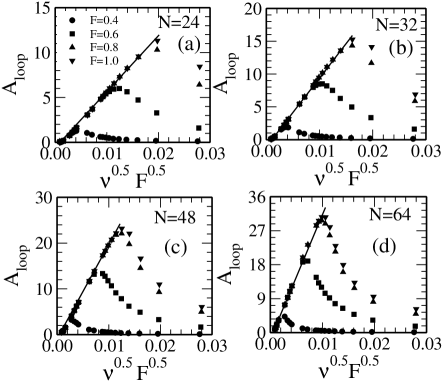
Figure 7: Figs (a-d) show the scaling of loop area of hysteresis with respect to $\nu^{0.5}F^{0.5}$ for different lengths. It is evident from all these plots that in low frequency limit curves of different amplitudes collapse on a single line intricating that the dynamical transition may exist in the thermodynamic limit.

For the spin systems, the area under the hysteresis loop ($A_{loop}\sim h^{\alpha}\nu^{\beta}$) is the measure of energy dissipated over a cycle. In a recent paper, Kumar and Mishra arxiv1 for a small dsDNA ($N_{p}=16$ base pairs) found a similar scaling for DNA unzipping i.e. the area of hysteresis loop scales with $F^{\alpha}\nu^{\beta}$. In low frequency regime, value of $\alpha$ and ${\beta}$ are found to be equal to $0.5$, which are same as one obtained in the case of isotropic spin system dd . At high frequency, the values of $\alpha$ and $\beta$ are found to be $2$ and $-1$, respectively, which are also consistent with isotropic spin system. In order to see whether these scaling holds for different lengths, we measured the area of hysteresis loop for the various chain length of DNA ($N=24,32,48$ and $64$) and plotted it with $F^{0.5}\nu^{0.5}$ in the low frequency regime (Fig. 7 a-d) and $(F-f_{c})^{2.0\pm 0.1}\nu^{-1}$ in the high frequency regime (Fig. 8 a-d). Here, $f_{c}$ is the equilibrium critical force at that temperature (Fig. 3). For all lengths studied here, the collapse of data for different $F$ on a single curve in low and high frequency regimes, suggest that the dynamical transition may be seen in single molecule experiments, which involve chain of finite size.

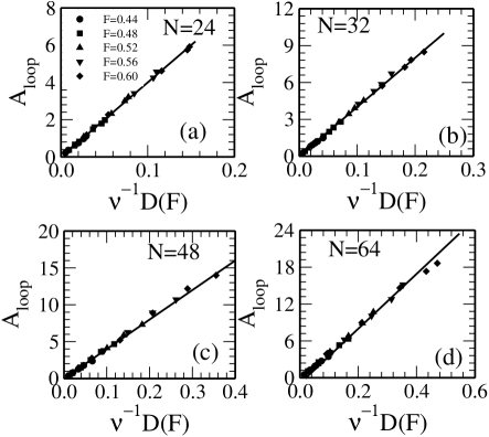
Figure 8: Same as Fig.7, but loop area of hysteresis has been plotted with respect to $\nu^{-1.0}D(F)$. Here D(F) $\sim$ $(F-f_{c})^{2.0\pm 0.1}$. In high frequency regime also, curves of different length of DNA collapse on a single line.

We now focus our study to SIP under a periodic force, where a bead (or monomer) can interact with the rest of non-bonded monomers. It is interesting to note that in low as well as in high frequency regimes, the SIP also obey the similar scaling as shown in the Fig. 9 a & b with the same scaling exponents.

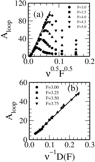
Figure 9: (a) Same as of Fig. 7, but for the SIP. In low frequency regime, curves of different amplitudes collapse on a single line. (b) At high frequency, curves for different F collapse on a straight line. Here D(F) $\sim$ $(F-f_{c})^{2.0\pm 0.1}$.

V Finite size scaling

We have studied the average energy dissipated per monomer i.e. $A_{loop}/N$, over a cycle. In the limit $\nu\rightarrow 0$, we have plotted the $A_{loop}/N$ with $F^{0.5}\nu^{0.5}N^{0.75}$ in Fig. 10. One can see the collapse of data for all lengths of different forces and frequencies. Similarly, Fig. 11 shows the collapse of data of all lengths in high frequency regime. It is interesting to note that in high frequency regime the average dissipated energy ($A_{loop}$) is independent of length. This may be understood by realizing that the applied force will try to move the end terminal with a velocity $v$. For a very short duration of time ($\nu\rightarrow\infty$), the applied force can move the end terminal to a finite distance, which is independent of length. Hence, the area under a cycle of force (0 to $F$ and back to 0) will remain independent of length (Fig. 11). However, in low frequency regime ($\nu\rightarrow 0$), the system gets enough time (close to equilibrium). Because of the connectivity of the beads in the chain, the applied force will be transmitted all along the chain. Consequently, both strands will move under the periodic force and the resultant curve under hysteresis will depend on the length of the chain (Fig. 10).

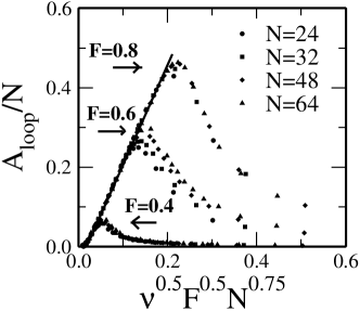
Figure 10: Figure shows the collapse of data for different lengths. In low frequency regime, curves of different amplitudes collapse on a single line.

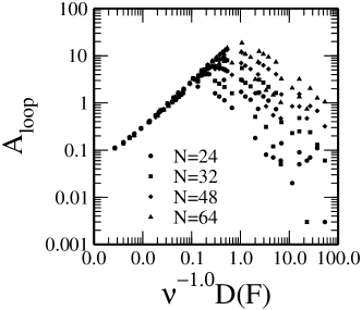
Figure 11: Figure shows that at high frequency, curves for different lengths collapse on a straight line. (For clarity we have plotted Fig.10 in log-log scale) Here, $D(F)$ has the same scaling form as mentioned in caption of Fig. 8.

VI Critical frequency and its dependence on $N$

From Fig. 5, it is clear that as frequency decreases, the system goes from one regime ($\nu^{-1}$) to the other ($\nu^{0.5}$). The frequency at which the area of hysteresis loop is maximum (discontinued) is termed as critical frequency $\nu_{c}$ dd . In Fig. 12 a, we have shown that the critical frequency decreases with N for a given value of $F$. In order to see its dependence on $N$, we investigate the dynamics of the system near $T=0$ under a linear ramp (triangular shape), similar to the one taken in our simulation arxiv1 . We assume here that there is no acceleration and beads move with a uniform velocity (because of environment) under the applied force. The contribution of random noise is negligible and Eq. 2 reduces to

$$\zeta\frac{d{\bf r}}{dt}={\bf F_{c}}+{\bf F}\nu t.$$ (4)

The frequency at which maximum area occurs, the extension $r$ scales as $N$. Since, $F$ is constant therefore $t$ also scales as $N$ and $\nu$ scales as $1/N$ to keep $\nu t$ constant. In Fig. 12 b, we have plotted $A/N$ with the scaled frequency $\nu^{*}=N\nu$. It is evident from Fig. 12 b that maxima of all lengths occur at critical frequency $\nu_{c}$ without changing the qualitative features of the curve. In low frequency regime, $A/N$ scales $\nu^{*0.5}$. One can see from the inset of Fig. 12c that the additional multiplication of $N^{0.25}$ with $\nu^{*0.5}$ gives a better collapse similar to the one shown in Fig.10. This may be a crossover or effect of random fluctuation because of finite temperature or the entropy associated with polymer chain, or the combined effect of all these, whose precise contributions have been ignored in Eq. 4.

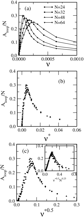
Figure 12: (a) Area of the loop per bead with frequency at fixed amplitude of force $0.6$. The peak of the curve shifts right with $N$. (b) Same as (a) but with scaled frequency $\nu^{*}=N\nu$. The peak of all the curves collapsed at frequency $\nu_{c}$. (c) In low frequency regime, $A/N$ scales as $\nu^{*0.5}$. The inset shows the scaling ($\nu^{*0.5}N^{0.25}$) of x-axis gives a better collapse.

VII conclusions

In this paper, we have investigated the dynamical transition associated with DNA and SIP. A simple model of a polymer developed here can describe some of the essential properties of bio-polymers (e.g. DNA and SIP) depending upon the interaction imposed on the non-bonded monomers. We have studied these two models under a periodic force and showed that they show similar behavior. Our studies provide strong evidence that in the low as well as in the high frequency regime, the area of hysteresis loop scales with the same exponents irrespective where a monomer interacts with native neighbor (DNA) or the non-native neighbor (SIP). The values of $\alpha$ and $\beta$ are consistent with the previous studies and have the same values as found in case of the isotropic spin systems dd . We have also shown that the value of these exponents remain the same for different lengths of DNA. In high frequency regime, area of the loop remains independent of length i.e. $\sim F^{2}\nu^{-1}$. In low frequency regime, we report a new scaling, where average energy dissipated per bead over a cycle scales as $F^{0.5}\nu^{0.5}N^{0.75}$. This suggests that the dynamical transition may be seen in single molecule experiments of finite chain. However, the present scaling is at finite temperature, where noise in Eq. 2 has an important role. It would be interesting to probe these scaling for a longer chain in the low temperature regime, where noise has no significant contribution. Our work calls for further investigations whether these exponents are universal for the other polymeric models or its value may differ e.g. for proteins and RNA, which have distinct structures.

VIII acknowledgments

We thank S. M. Bhattacharjee for many helpful discussions on the subject. Financial supports from the DST and CSIR, India are gratefully acknowledged. We also acknowledge the generous computer support from IUAC, New Delhi.

References

- (1) M. Shtilerman, G. H. Lorimer, and S. W. Englander Science, 284, 822 (1999).
- (2) S. Huang, K. S. Ratliff, M. P. Schwartz, J. M. Spenner, and A. Matouschek, Nat. Struct. Biol. 6, 1132 (1999).
- (3) A. F. Neuwald, L. Aravind, J. L. Spouge and E.V. Koonin Genome Res. 9, 27 (1999).
- (4) P. Cook, Science 284, 1790 (1999).
- (5) P. Guo and T. Lee, Mol. Microbiol. 64, 886 (2007).
- (6) B. Alberts, D. Bray, J. Lewis, M. Raff, K. Roberts and J. D. Watson, Molecular Biology of the Cell, (Garland Publishing: New York, 1994).
- (7) D. Tomkiewicz, N. Nouwen, and A. Driessen, FEBS Lett. 581, 2820 (2007).
- (8) I. Donmez and S. S. Patel, Nucl. Acids Res. 34, 4216 (2006).
- (9) M. E. Fairman-Williams and E. Jankowsky, J. Mol. Biol 415, 819 (2012).
- (10) M. Hochstrasser and J. Wang, Nat.Struct. Biol. 8, 294 (2001).
- (11) C. Lee, M. P. Schwartz, S. Prakash, M. Iwakura and A. Matouschek, Mol. Cell, 7, 627 (2001).
- (12) A. Navon and A. L. Goldberg, Mol. Cell, 8, 1339 (2001).
- (13) A. Vidybida, Acta Mech. 67, 183 (1987).
- (14) O.Braun, A. Hanke and U. Seifert, Phys. Rev. Lett. 93, 158105 (2004).
- (15) Y. Pereverzev and O. Prezhdo, Biophys. J. 91, L19 (2006).
- (16) M. Lomholt, M. Urbakh, R. Metzler and J. Klafter Phys. Rev. Lett. 98, 168302 (2007).
- (17) H. Lin, Y. Sheng, H. Chen and H. Tsao, J. Chem. Phys. 128, 084708 (2008).
- (18) S. Kumar and M. S. Li, Phys. Rep. 486, 1 (2010).
- (19) M. Rao and R. Pandit, Phys. Rev. B 43, 3373 (1991).
- (20) M. Rao, H. R. Krishnamurthy and R. Pandit, Phys. Rev. B 42, 856 (1990).
- (21) D. Dhar and P. Thomas, J. Phys. A 25, 4967 (1992).
- (22) B. K. Chakrabarti and M. Acharyya, Rev. Mod. Phys. 71, 847 (1999).
- (23) G. H. Goldsztein, F. Broner and S. H. Strogatz, Siam J. Appl. Math. 57 1163 (1997).
- (24) J. Liphardt, S. Dumont, S. B. Smith, I. Tinoco, Jr. and C. Bustamante, Science 296, 1832 (2002).
- (25) D. Collin, F. Ritort, C. Jarzynski, S. B. Smith, I. Tinoco, Jr. and C. Bustamante, Nature 437, 231 (2005).
- (26) M. Schlierf, F. Berkemeier and M. Rief, Biophys. J. 93, 3989 (2007).
- (27) K. Hatch, C. Danilowicz, V. Coljee and M. Prentiss, Phys. Rev. E 75, 051908 (2007).
- (28) P. T. X. Li, C. Bustamante and I. Tinoco, Jr., PNAS 104, 7039 (2007).
- (29) T. Bornschlögl and M. Rief, Langmuir 24, 1338 (2008).
- (30) R. W. Friddle, P. Podsiadlo, A. B. Artyukhin, and A. Noy, J. Phys. Chem. C 112, 4986 (2008).
- (31) G. Diezemann and A. Janshoff, J. Chem. Phys. 129, 084904 (2008).
- (32) R. Kapri Phys. Rev. E 86, 041906 (2012).
- (33) P. Sadhukhan and S. M. Bhattacharjee, J. Phys. A 43, 245001 (2010).
- (34) G. Mishra, P. Sadhukhan, S. M. Bhattacharjee and S. Kumar, Phys. Rev. E 87, 022718 (2013).
- (35) S. Kumar and G. Mishra arxiv: 1208.5126 (2012).
- (36) S. Kumar, I. Jensen, J. L. Jacobsen and A. J. Guttmann, Phys. Rev. Lett. 98, 128101 (2007).
- (37) M. P. Allen and D. J. Tildesley, Computer simulations of liquids (Oxford Science, 1987).
- (38) D. Frenkel and B. Smit, Understanding molecular simulation (Academic Press, London, 2002).
- (39) M. S. Li and M. Cieplak, Phys. Rev E 59, 970 (1999).
- (40) M. Kouza et al Biophys. J. 89, 3353 (2005).
- (41) M. S. Li, Biophys. J. 93, 2644 (2007).
- (42) C. Hyeon and D. Thirumalai, PNAS 102, 6789 (2005).
- (43) G. Mishra, D. Giri, M. S. Li and S. Kumar, J. Chem. Phys 135, 035102 (2011).
- (44) M. Ciesla, J. Pawlowicz, L. Longa, ACTA Physica Polonica B 38,(2007).
- (45) N. Go and H. Abe, Biopolymers 20, 991 (1981).
- (46) D. Poland and H.A. Scheraga, J. Chem. Phys. 45, 1456 (1966); ibid 45, 1464 (1966).
- (47) N. Singh and S. Srivastava, J. Chem. Phys. 134, 115102 (2011).
- (48) D. Foster and C. Pinetter, Phys. Rev. E 79, 051108 (2009).
- (49) E. J. Sambriski, V. Ortiz and J. J. de Pablo, J. Phys.: Cond. Mat. 21 034105 (2009).
- (50) G. E. P. Box and G. M. Jenkins, Time series analysis: Forecasting and Control, p28, Holden-day, San Francisco, (1970); Y. S. lee and T. Ree, Bull. Korean Chem. Soc. 3, 44 (1982).
- (51) B. A. Berg in Markov Chain Monte Carlo: Innovations and Applications, Eds. W. S. Kendall, F. Liang and J-S. Wang, Page 1, World Scientific, Singapore (2005).
- (52) S. M. Bhattacharjee, J. Phys. A, 33, L423 (2000).
- (53) D. Marenduzzo et al., Phys. Rev. Lett. 88, 028102 (2001).