Non-Gaussian Minkowski functionals & extrema counts
in redshift space

Abstract

In the context of upcoming large-scale structure surveys such as Euclid, it is of prime importance to quantify the effect of peculiar velocities on geometric probes. Hence the formalism to compute in redshift space the geometrical and topological one-point statistics of mildly non-Gaussian 2D and 3D cosmic fields is developed. Leveraging the partial isotropy of the target statistics, the Gram-Charlier expansion of the joint probability distribution of the field and its derivatives is reformulated in terms of the corresponding anisotropic variables. In particular, the cosmic non-linear evolution of the Minkowski functionals, together with the statistics of extrema are investigated in turn for 3D catalogues and 2D slabs. The amplitude of the non-Gaussian redshift distortion correction is estimated for these geometric probes. In 3D, gravitational perturbation theory is implemented in redshift space to predict the cosmic evolution of all relevant Gram-Charlier coefficients. Applications to the estimation of the cosmic parameters $\sigma(z)$ and $\beta=f/b_{1}$ from upcoming surveys is discussed. Such statistics are of interest for anisotropic fields beyond cosmology.

1 Introduction

In modern cosmology, random fields (3D or 2D) are fundamental ingredients in the description of the large-scale matter density and the Cosmic Microwave Background (CMB). The large-scale structure of the matter distribution in the Universe is believed to be the result of the gravitational growth of primordial nearly-Gaussian small perturbations originating from quantum fluctuations. Deviations from Gaussianity inevitably arise due to the non-linear dynamics of the growing structures, but may also be present at small, but potentially detectable levels in the initial seed inhomogeneities. Thus, studying non-Gaussian signatures in the random fields of cosmological data provides methods to learn both the details of early Universe’s physics and mechanisms for structure’s growth, addressing issues such as the matter content of the Universe (Zunckel et al., 2011), the role of bias between galaxies and dark matter distributions (Desjacques & Sheth, 2010), and whether it is dark energy or a modification to Einstein’s gravity (Wang et al., 2012) that is responsible for the acceleration of the Universe’s expansion.

With upcoming high-precision surveys, it has become necessary to revisit alternative tools to investigate the statistics of random cosmological fields so as to handle observables with different sensitivity. Minkowski functionals (Mecke et al., 1994) have been being actively used (Gott et al., 1987; Weinberg et al., 1987; Melott et al., 1988; Gott et al., 1989; Hikage et al., 2002, 2003; Park et al., 2005; Gott et al., 2007; Planck Collaboration et al., 2013) as an alternative to the usual direct measurements of higher-order moments and N-point correlation functions (Scoccimarro et al., 1998; Percival et al., 2007; Gaztañaga et al., 2009; Nishimichi et al., 2010, amongst many other studies) as they will present different biases and might be more robust, e.g. with regards to rare events. These functionals are topological and geometrical estimators involving the critical sets of the field. As such they are invariant under a monotonic transformation of the field (and in particular bias-independent if the bias is monotonic!). If their expression for Gaussian isotropic fields has long been known (Doroshkevich, 1970; Adler, 1981; Bardeen et al., 1986; Hamilton et al., 1986; Bond & Efstathiou, 1987; Ryden, 1988; Ryden et al., 1989), their theoretical prediction have also been computed more recently for mildly non-Gaussian fields (Matsubara (1994), Pogosyan et al. (2009) and Matsubara (2010) for the first and second non-Gaussian corrections using a multivariate Edgeworth expansion, and more recently by Gay et al. (2012) to all orders in non-Gaussianity). However, one major assumption in these results has been the isotropy of the underlying field.

Indeed, the assumptions of homogeneity and isotropy of our observable Universe are central to our understanding of the universe. This focuses our primary attention on statistically homogeneous and isotropic random fields as the description of cosmological 2D and 3D data. These statistical symmetries provide essential guidance for the theoretical description of the geometry of the cosmological random fields. Recent papers (Pogosyan et al., 2009, 2011; Gay et al., 2012) leverage the isotropy of the target statistics to develop non-Gaussian moment expansion to all orders for popular and novel statistics such as the above-mentioned Minkowski functionals, but also extrema counts and the skeleton of the filamentary structures. This formalism, generalizing the earlier works (Bardeen et al., 1986; Matsubara, 1994, 2003; Pogosyan et al., 2009), allows for controlled comparison of the non-Gaussian deviations of geometrical measures in theoretical models, simulations, and the observations, assuming homogeneity and isotropy. Nevertheless, 3D surveys are conveyed in redshift space where the hypothesis of isotropy breaks down. Indeed in astrophysical observations, the three dimensional positions of structures are frequently not accessible directly. While angular positions on the sky can be obtained precisely, the radial line-of-sight (hereafter LOS) position of objects is determined by proxy, e.g., via measurements of the LOS velocity component. This implies that galaxy distribution data are presented in redshift space in cosmological studies.

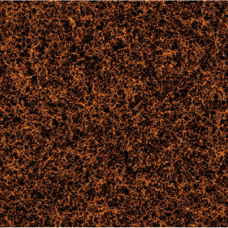
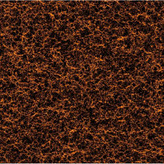
Figure 3: A slice through the horizon $4\pi$ halo catalog at redshift zero without (left panel) and with (right panel) redshift distortion (along the ordinate). The boxsize is 2 Gpc$/h$, the slice thickness 40 Mpc$/h$. The area is 20$\times$20 larger than the slice presented in Figure 1. Each dot represents a halo colour-coded by its mass. Note the clear preferred horizontal elongation of structures in redshift space.

Figures 1 and 3 illustrates the amplitude of such redshift distortion as a function of scale. On small, non-linear scales, the well-known finger-of-God effect (Jackson, 1972; Peebles, 1980) stretches the collapsing clusters along the line-of-sight whereas on larger scales (see Figure 3) the redshift space distortion flattens the voids along the LOS (Sargent & Turner, 1977), in accordance to the linear result of Kaiser (1987).

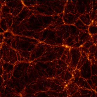
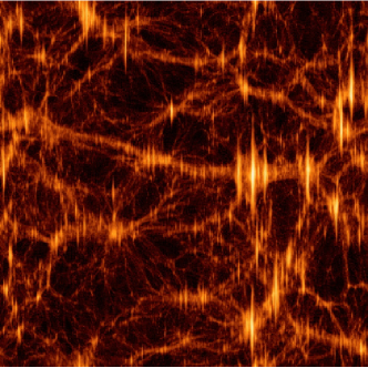
Figure 1: Left panel: an example of a slice through a $512^{3}$ dark matter particles $\Lambda$CDM simulations at redshift 0 ($\Omega_{m}=0.3$, $\Omega_{\Lambda}=0.7$, $\sigma_{8}=0.92$) in real space. The boxsize is 100 Mpc$/h$, the slice thickness 10 Mpc$/h$. Right panel shows the same field when redshift distortion has been applied along the ordinate. Fingers of God are quite visible on that slice (see also Figure 3).

But anisotropy in data does not affect only cosmological surveys: this issue is ubiquitous in physics: e.g neutral hydrogen distribution is mapped in Position-Position-Velocity cubes in studies of the interstellar or intergalactic medium, and turbulent distribution of magnetic field are mapped via Faraday rotation measure of the synchrotron emission (Heyvaerts et al., 2013). Thus, as a rule, the underlying isotropy of structures in real space is broken in the space where data is available. Hence developing techniques to recover properties of underlying fields from distorted datasets, anisotropic in the LOS direction, is a fundamental problem in astrophysics.

In this paper we thus present a theory of the non-Gaussian Minkowski functionals and extrema counts for $z$-anisotropic cosmological fields, targeted for application to data sets in redshift space in the so-called plane-parallel approximation. Hence this theory is a generalization of the formalism for mildly non-Gaussian but isotropic fields of Pogosyan et al. (2009); Gay et al. (2012) on one hand, and the theory of anisotropic redshift space effects on statistics in Gaussian limit developed in Matsubara (1996) on the other hand. The effects of anisotropy and non-Gaussianity are simultaneously important for a precise description of the large scale structures of the Universe (LSS hereafter) as mentioned in Matsubara & Suto (1995), where N-body simulations suggest that redshift space distortion has noticeable impact on the shape of the genus curve in the weakly non-linear regime. At the same time the theory presented in this paper is general and applicable to mildly non-Gaussian homogeneous and statistically axisymmetric random fields of any origin, for example for extending Velocity Channel Analysis of HI maps (Lazarian & Pogosyan, 2000) to account for non-Gaussian density compressibility, or describing cosmological perturbations in anisotropic Bianchi models of the Universe.

As an anticipation, Figure 2 illustrates the importance of modelling appropriately the anisotropy on the particular example of the 3D Euler characteristics of a mildly non-Gaussian scale-invariant cosmological field. Indeed, the theoretical prediction assuming isotropy given in equation (38) below (in purple) significantly fails to describe the measurement unlike the prediction proposed in equation (35) (in red). This suggests that in redshift space it is of great importance to properly account for anisotropy. This will be the topic of this paper.

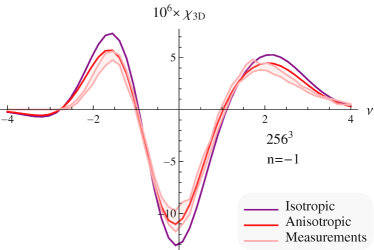
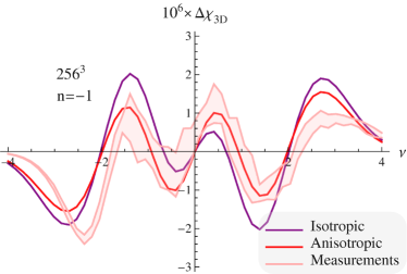
Figure 2: Left panel: 3D Euler characteristic of a mildly non-Gaussian scale invariant cosmological field ($n=-1,f=1$, $\sigma=0.18$). The prediction to first order in non-Gaussianity given by equation (35) corresponds to the red solid line and the prediction assuming isotropy (see equation (38)) to the purple line. The one sigma shaded area is the measurement. Right panel: same as left panel for the first order correction to the Gaussian distribution only.

Section 2 defines the statistics used in this paper, namely Minkowski functionals and critical points counts. Section 3 introduces the formalism to deal with the joint probability density function of the density field and its derivatives up to second order in redshift space. In particular, it shows how rotational invariance is used to introduce a relevant set of variables which diagonalizes the Gaussian JPDF; a Gram-Charlier expansion of the non-Gaussian JPDF is written there. Section 4 presents Minkowski functionals and extrema counts in 2 and 3D. Section 4.2 presents the full non-Gaussian expression for 3D and 2D Euler characteristic in redshift space, while section 4.3 is devoted to the last three Minkowski functionals (Area of isosurfaces, length of isocontours and contour crossing) for which we present expressions in redshift space up to first order in non-Gaussianity. Section 4.4 sketches the derivation for extrema counts in two and three dimensions. Section 4.5.1 re-expresses these functionals as a function of the filling factor threshold, while Section 4.5.2 investigates the implications of the topological invariance for the corresponding set of cumulants of the field. Section 5 analyses implication for the estimation of cosmological parameters. It shows how to compute the relevant three point cumulants in redshift space (e.g. skewness and its generalization to the derivatives of the density field) at tree order within perturbation theory (PT). In particular, it provides a way to compute analytically the angular part of the integrals under consideration. It then discusses which features of the bispectrum are robustly measured using these non-Gaussian critical sets and sketches two main applications: measuring $\sigma$ (hence dark energy) of the possibly masked underlying field, and measuring $\beta\equiv f/b_{1}\simeq\Omega_{m}^{0.55}/b_{1}$. Appendix A lists properties of the relevant cumulants. Appendix B presents briefly a set of “$f_{\mathrm{{nl}}}$” anisotropic non-Gaussian field toy models which we use to validate our theory. Finally Appendix C derives the 3D Euler characteristic at all orders in non-Gaussianity.

2 Geometrical statistics in 2 and 3D

Our prime focus is the geometrical and topological properties of cosmological fields. One way to probe these is to look at isocontours of the field at different thresholds and use Minkowski functionals to describe them (Mecke et al., 1994). These Minkowski functionals are known to be the only morphological descriptors in Integral Geometry that respect motion-invariance, conditional continuity and additivity (Hadwiger, 1957). As a result, they form a robust and meaningful set of observables. In $d$ dimensions, there are $d+1$ such functionals (4 in 3D and 3 in 2D), namely in 3D: the encompassed volume, $f_{V}$, the surface area, ${\cal N}_{3}$, the integral mean curvature and the integral Gaussian curvature (closely related to the Euler-Poincaré characteristic, $\chi$). For random fields these functionals are understood as densities, i.e quantities per unit volume of space.

Especially when studying anisotropic field, complimentary information can be obtained by using the geometrical statistics and Minkowski functionals for the field obtained on lower dimensional sections of the 3D field. For example, in addition to 3D isocontour area statistics, one can introduce the length of 2D isocontours on a planar sections ${\cal N}_{2}$, and contour crossings by a line through 3D space, ${\cal N}_{1}$. These statistics for cosmology were first introduced by Ryden (1988); Ryden et al. (1989). In the isotropic limit, they are trivially related: $2{\cal N}_{1}=4{\cal N}_{2}/\pi={\cal N}_{3}$; this relation does not hold anymore for an anisotropic field as it will be shown in sections 4.3.1, 4.3.2 and 4.3.3. Similarly, in addition to the full Euler characteristic $\chi_{\mathrm{3D}}$ of 3D excursion sets, we shall consider the 2D Euler characteristic, $\chi_{\mathrm{2D}}$, on planar sections through the field.

All geometrical measures can be expressed as averages over the joint probability density function (JPDF) of the field and its derivatives. In the following, let us call $x$ the field under consideration and, without loss of generality, assume that it has zero mean. In cosmological applications, this field, for instance, can be the 3D density contrast. Collecting the well-known results from an extensive literature (e.g. Rice, 1944, 1945; Ryden, 1988; Matsubara, 1996) in a compact form, we have for the first two Minkowski functionals

$$f_{V}(\nu) = \left\langle\Theta(x-\nu)\right\rangle\leavevmode\nobreak\ \leavevmode\nobreak\ ,$$ (1)

$${\cal N}_{3}(\nu)\!\! = \left\langle|\nabla x|\delta_{\mathrm{D}}(x-\nu)\right\rangle\,,\quad{\cal N}_{2}(\nu)=\left\langle|\nabla_{\!{\cal S}}\,x|\delta_{\mathrm{D}}(x-\nu)\right\rangle\,,\quad{\cal N}_{1}(\nu)=\left\langle|\nabla_{\!{\cal L}}\,x|\delta_{\mathrm{D}}(x-\nu)\right\rangle\,,$$ (2)

where the $\delta_{\rm D}$-function in the statistical averaging signifies evaluation at the given threshold $x=\nu$, while the step function reflects the cumulative averaging over the values above the threshold $x\geq\nu$. We see that the family of threshold-crossing statistics is given by the average gradient of the field for ${\cal N}_{3}$ or its restriction to the plane ${\cal S}$ or line ${\cal L}$ for ${\cal N}_{2}$ and ${\cal N}_{1}$, respectively.

The average of the Gaussian curvature on the isosurface is, via the Gauss-Bonnet theorem, its topological Euler characteristic $\chi$, which thus can be expressed directly as $\chi(\nu)=\left\langle\delta_{\mathrm{D}}(x-\nu)\delta_{\mathrm{D}}(\nabla_{1}x)\delta_{\mathrm{D}}(\nabla_{2}x)|\nabla_{3}x|(\nabla_{1}\nabla_{1}x\nabla_{2}\nabla_{2}x-(\nabla_{1}\nabla_{2}x)^{2})\right\rangle$ (Hamilton et al., 1986; Matsubara, 1996). In this paper we use the Euler characteristic, $\chi_{\mathrm{3D}}$, of the excursion set encompassed by the isosurface (which in 3D is just one half of the Euler charasteristic of the isosurface itself, and is equal to minus the genus for the definitions used in cosmology, see detailed discussions for such conventions in Gay et al. (2012)). Being the alternating sum of Betti numbers, $\chi_{\mathrm{3D}}$ is related via Morse theory (e.g., Jost, 2008) to the alternating sum of the number of critical points in the excursion volume. For a random field (Doroshkevich, 1970; Adler, 1981; Bardeen et al., 1986)

$$\chi_{3\mathrm{D}}(\nu)\!\!=-\left\langle\det\!\left({\nabla_{i}\nabla_{j}x}\right)\delta_{\mathrm{D}}(\nabla x)\Theta(x-\nu)\right\rangle\;,\quad i,j\in\{1,2,3\}\,.$$ (3)

The Euler characteristic of the excursion sets of a 2D field (in particular, 2D slices of a 3D random field) is given by a similar expression (Adler, 1981; Bond & Efstathiou, 1987; Coles, 1988; Melott et al., 1989; Gott et al., 1990)

$$\chi_{2\mathrm{D}}(\nu)\!\!=\left\langle\det\!\left({\nabla_{i}\nabla_{j}x}\right)\delta_{\mathrm{D}}(\nabla x)\Theta(x-\nu)\right\rangle\;,\quad i,j\in\{1,2\}\,.$$ (4)

For an anisotropic 3D field along the third direction, $\chi_{\mathrm{2D}}$ depends on the angle $\theta_{\cal S}$ between this direction and the plane (${\cal S}$) under consideration (Matsubara, 1996). equation (4) is then understood as

$$\chi_{2\mathrm{D}}(\nu,\theta_{\cal S})=\left\langle\det\!\left({\tilde{\nabla}_{i}\tilde{\nabla}_{j}x}\right)\delta_{\mathrm{D}}(\tilde{\nabla}x)\Theta(x-\nu)\right\rangle\;,\quad i,j\in\{1,2\},$$ (5)

where $\tilde{\nabla}$ is the gradient on the plane i.e. $\tilde{\nabla}_{1}=\nabla_{1}$ and $\tilde{\nabla}_{2}=\sin\theta_{\cal S}\nabla_{2}+\cos\theta_{\cal S}\nabla_{3}$. The freedom associated with the choice of plane will be further discussed in Section 5.

With the same formalism, it is easy to compute the critical points counts (Adler, 1981; Bardeen et al., 1986). Equation (3) leads to a cumulative counting above a given threshold for maxima, two type (filamentary and wall-like) saddle points and minima

$$n_{\mathrm{max,3\mathrm{D}}}(\nu) = -\left\langle\det\!\left({\nabla_{i}\nabla_{j}x}\right)\delta_{\mathrm{D}}(\nabla x)\Theta(-\lambda_{1})\Theta(x-\nu)\right\rangle,$$ (6)

$$n_{\mathrm{sadf,3\mathrm{D}}}(\nu) = +\left\langle\det\!\left({\nabla_{i}\nabla_{j}x}\right)\delta_{\mathrm{D}}(\nabla x)\Theta(\lambda_{1})\Theta(-\lambda_{2})\Theta(x-\nu)\right\rangle,$$ (7)

$$n_{\mathrm{sadw,3\mathrm{D}}}(\nu) = -\left\langle\det\!\left({\nabla_{i}\nabla_{j}x}\right)\delta_{\mathrm{D}}(\nabla x)\Theta(\lambda_{2})\Theta(-\lambda_{3})\Theta(x-\nu)\right\rangle,$$ (8)

$$n_{\mathrm{min,3\mathrm{D}}}(\nu) = +\left\langle\det\!\left({\nabla_{i}\nabla_{j}x}\right)\delta_{\mathrm{D}}(\nabla x)\Theta(\lambda_{3})\Theta(x-\nu)\right\rangle\,,$$ (9)

where averaging conditions are set by the signs of sorted eigenvalues $\lambda_{1}\geq\lambda_{2}\geq\lambda_{3}$ of the Hessian matrix of the field. Taking alternating sum eliminates the constraints on signs of eigenvalue, leading to the $\chi_{\mathrm{3D}}$ statistics. Similar expressions as equations (6)-(9) apply for 2D extrema.

Extrema counts provide us with information on peaks (dense regions), minima (under-dense regions), and saddle points. In some applications there is symmetry between extrema (e.g. in CMB studies minima and maxima of the temperature field are equivalent); in others, they describe very different structures, e.g. in LSS dense peaks correspond to graviationally collapsing objects like galactic or cluster haloes while minima seed the regions devoid of structures. Saddle-type extrema are also interesting in their own right, being related to the underlying filamentary structures (bridges connecting peaks through saddles), which in turn can also be characterized by the skeleton (Novikov et al., 2003; Gay et al., 2012) of the Cosmic Web. A particular advantage of the described geometrical statistical estimates is that they are invariant under monotonic transformation of the underlying field $x\to f(x)$, provided one maps the threshold correspondingly $\nu\to f(\nu)$. For cosmological data this means that these statistics are formally invariant with respect to any monotonic local bias between the galaxy and matter distributions. We demonstrate this formally, order by order, in section 4.5.2.

3 The joint PDF: rotational invariance and Gram-Charlier expansion

Evaluating the expectations in equations (1-9) requires a model for the joint probability distribution function (JPDF) of the field and its derivative up to second order, $P(x,\nabla_{i}x,\nabla_{i}\nabla_{j}x)$. Let us now proceed to developing this JPDF for a mildly non-Gaussian and anisotropic field such as the cosmological density field in redshift space, starting with a formal definition of redshift space.

3.1 Statistically anisotropic density field in redshift space

In an astrophysical context, we focus on the statistics of isodensity contours of matter in the redshifted Universe. The estimation of position via redshift assigns to a given object the “redshift” coordinate, ${\bf s}$,

$${\bf s}={\bf r}+H^{-1}{\bf v}\cdot{\bf\hat{r}}$$ (10)

shifted from the true position ${\bf r}$ by the projection of the peculiar velocity ${\bf v}$ along the line-of-sight direction ${\bf\hat{r}}$.

On large scales, in the linear regime of density evolution, the mapping to redshift coordinates induces an anisotropic change in mass density contrast (Kaiser, 1987), best given in Fourier space

$$\hat{\delta}^{(s)}(\mathbf{k})=(1+f\mu^{2})\hat{\delta}^{(r)}(\mathbf{k}),$$ (11)

that has dependency on the angle $\mu={\bf k}\cdot{\bf\hat{r}}/k$ between the direction of the wave ${\bf k}$ and the line of sight, and the amplitude, $f$, tracing the growth history of linear inhomogeneities $D(a)$, $f=\mathrm{d}\log D/\mathrm{d}\log a\approx\Omega_{m}^{0.55}$, (Peebles, 1980). The main qualitative effect of this distortion is the enhancement of clustering via the squeezing overdense regions and the stretching underdense voids along the line of sight. If matter is traced by biased halos (e.g. galaxies), the redshift space distortion $\delta_{g}$ can be modeled by a linear bias $b_{1}$ factor (Kaiser, 1984)

$$\hat{\delta}_{g}^{(s)}(\mathbf{k})=(1+\beta\mu^{2})\hat{\delta}_{g}^{(r)}(\mathbf{k})\,,\quad\beta\equiv f/b_{1}\,.$$ (12)

Depending on context, we shall use either $f$ or $\beta$ to parametrize the linearized redshift distortions, and either equation (11) or (12) to generate maps.

In the mildly non-linear regime, the focus of this investigation, redshift distortions interplay with non-Gaussian corrections that develop with the growth of non-linearities. Scoccimarro et al. (1999); Bernardeau et al. (2002) established the framework for a perturbative approach to this regime, which we built upon in Section 5.3. In redshift space, the density field is statistically anisotropic, with line-of-sight expectations differing from expectations in the perpendicular directions (in the plane of the sky). We shall consider the Minkowski functionals and extrema statistics in the plane-parallel approximation, where the LOS direction is identified with the Cartesian third, “$z$”, coordinate. As the first step, we extend the non-Gaussian formalism introduced in Pogosyan et al. (2009); Gay et al. (2012) to partly anisotropic, axisymmetric fields, establishing several formal results for all orders in non-Gaussianity.

3.2 3D formalism

Following Pogosyan et al. (2009), we choose a non-Gaussian Gram-Charlier expansion of the JPDF (Cramér, 1946; Kendall & Stuart, 1958; Chambers, 1967; Juszkiewicz et al., 1995; Amendola, 1996; Blinnikov & Moessner, 1998) (for a first application to CMB see, e.g., Scaramella & Vittorio (1991)) using polynomial variables that are invariant with respect to the statistical symmetries of the field. In the presence of anisotropy in the direction along the LOS, all statistical measures should be independent with respect to sky rotations in the plane perpendicular to the LOS.

Let us denote the field variable as $x$ for the density contrast and $x_{i}$, $x_{ij}$ for its first and second derivatives. These field variables are separated into the following groups based on their behaviour under sky rotation: $x$ and $x_{33}$ are scalars, $x_{3}$ is a pseudoscalar, $(x_{1},x_{2})$ and $(x_{13},x_{23})$ are two vectors and $(x_{11},x_{22},x_{12})$ is a symmetric $2\times 2$ tensor. We can construct eight 2D sky rotation invariant polynomial quantities: four linear ones $x$, $x_{33}$, $x_{3}$ and $J_{1\perp}\equiv x_{11}+x_{22}$; three quadratic: $q^{2}_{\perp}\equiv x_{1}^{2}+x_{2}^{2}$, $Q^{2}\equiv x_{13}^{2}+x_{23}^{2}$ and $J_{2\perp}\equiv(x_{11}-x_{22})^{2}+4x_{12}^{2}$; and one cubic, $\Upsilon\equiv\left(x_{13}^{2}-x_{23}^{2}\right)\left(x_{11}-x_{22}\right)+4x_{12}x_{13}x_{23}$, which is directly related to the 2D polar angle $\psi$ between $(x_{13},x_{23})$ vector and the eigendirection of the $(x_{11},x_{22},x_{12})$ matrix , $\Upsilon=Q^{2}\sqrt{J_{2\perp}}\cos 2\psi$.

To build the Gram-Charlier expansions, we start with the Gaussian limit to the one-point JPDF of all the invariant variables, which then serves as a kernel for defining orthogonal polynomials into which the deviations from Gaussianity are expanded (see Gay et al. (2012) for further details). The Gaussian limit is determined as the limit in which distribution of field variables $x,x_{i},x_{ij}$ is approximated by Gaussian JPDF. The field variables are defined to have zero mean. Their covariance matrix in anisotropic case contains the variances, defined as

$$\left\langle x^{2}\right\rangle\equiv\sigma^{2},\leavevmode\nobreak\ \leavevmode\nobreak\ \left\langle x_{1}^{2}\right\rangle=\left\langle x_{2}^{2}\right\rangle\equiv\frac{1}{2}\sigma_{1\perp}^{2},\leavevmode\nobreak\ \leavevmode\nobreak\ \left\langle x_{3}^{2}\right\rangle\equiv\sigma_{1\parallel}^{2},$$

$$\left\langle x_{11}^{2}\right\rangle=\left\langle x_{22}^{2}\right\rangle\equiv\frac{3}{8}\sigma_{2\perp}^{2},\leavevmode\nobreak\ \leavevmode\nobreak\ \left\langle x_{12}^{2}\right\rangle\equiv\frac{1}{8}\sigma_{2\perp}^{2},\leavevmode\nobreak\ \leavevmode\nobreak\ \left\langle x_{33}^{2}\right\rangle\equiv\sigma_{2\parallel}^{2},\leavevmode\nobreak\ \leavevmode\nobreak\ \left\langle x_{13}^{2}\right\rangle=\left\langle x_{23}^{2}\right\rangle\equiv\frac{1}{2}\sigma_{Q}^{2},$$ (13)

and the cross-correlations, amongst which the non-zero are

$$\langle xx_{11}\rangle=\langle xx_{22}\rangle\equiv-\frac{1}{2}\sigma_{1\perp}^{2},\leavevmode\nobreak\ \leavevmode\nobreak\ \langle xx_{33}\rangle\equiv-\sigma_{1\parallel}^{2},\leavevmode\nobreak\ \leavevmode\nobreak\ \langle x_{11}x_{22}\rangle\equiv\frac{1}{8}\sigma_{2\perp}^{2},\leavevmode\nobreak\ \leavevmode\nobreak\ \langle x_{11}x_{33}\rangle=\langle x_{22}x_{33}\rangle=\frac{1}{2}\sigma_{Q}^{2}.$$ (14)

These properties translate into the following lowest moments for 2D rotation invariant quantities

$$\langle x\rangle=\langle J_{1\perp}\rangle=\langle x_{33}\rangle=\langle\Upsilon\rangle=0,\leavevmode\nobreak\ \leavevmode\nobreak\ \left\langle x^{2}\right\rangle=\sigma^{2},\leavevmode\nobreak\ \leavevmode\nobreak\ \langle J_{1\perp}^{2}\rangle=\sigma_{2\perp}^{2},\leavevmode\nobreak\ \leavevmode\nobreak\ \left\langle x_{33}^{2}\right\rangle=\sigma_{2\parallel}^{2},\leavevmode\nobreak\ \leavevmode\nobreak\ \langle q^{2}_{\perp}\rangle=\sigma_{1\perp}^{2},\leavevmode\nobreak\ \leavevmode\nobreak\ \left\langle Q^{2}\right\rangle=\sigma_{Q}^{2},\leavevmode\nobreak\ \leavevmode\nobreak\ \left\langle J_{2\perp}\right\rangle=\sigma_{2\perp}^{2}.$$ (15)

The cross-correlations of invariants are limited to the $x,J_{1\perp},x_{33}$ subset, $\left\langle xJ_{1\perp}\right\rangle=-\sigma_{1\perp}^{2}$, $\left\langle xx_{33}\right\rangle=-\sigma_{1\parallel}^{2}$, $\left\langle J_{1\perp}x_{33}\right\rangle=\sigma_{Q}^{2}$ and the coupling of $\Upsilon$ with $Q^{2}$ and $J_{2\perp}$. The scalar part of the gradient $x_{3}$ remains uncorrelated with the rest of the variables due to its pseudo-scalar nature (changing sign when $z$ flips). From now on, we shall consider field variables to be normalized by the corresponding $\sigma$, $\sigma_{1\perp}$, $\sigma_{1\parallel}$, $\sigma_{2\perp}$, $\sigma_{2\parallel}$ and $\sigma_{Q}$. The linear invariant combinations are normalized by their standard deviations and the quadratic ones by their mean values. Correlations are then described by the dimensionless coefficients $\gamma_{\perp}\equiv\sigma_{1\perp}^{2}/(\sigma\sigma_{2\perp})$, $\gamma_{\parallel}\equiv\sigma_{1\parallel}^{2}/(\sigma\sigma_{2\parallel})$ and $\gamma_{2}\equiv\sigma_{Q}^{2}/(\sigma_{{2}\perp}\sigma_{{2}\parallel})$, corresponding to generalized shape parameters (Bernardeau et al., 2002). Note that in the isotropic limit,

$$\sigma^{2}_{1\perp}=2/3\sigma^{2}_{1},\leavevmode\nobreak\ \leavevmode\nobreak\ \leavevmode\nobreak\ \sigma^{2}_{1\parallel}=1/3\sigma^{2}_{1},\leavevmode\nobreak\ \leavevmode\nobreak\ \leavevmode\nobreak\ \sigma^{2}_{2\perp}=8/15\sigma^{2}_{2},\leavevmode\nobreak\ \leavevmode\nobreak\ \leavevmode\nobreak\ \sigma^{2}_{2\parallel}=1/5\sigma^{2}_{2},\leavevmode\nobreak\ \leavevmode\nobreak\ \leavevmode\nobreak\ \sigma^{2}_{Q}=2/15\sigma^{2}_{2},\leavevmode\nobreak\ \leavevmode\nobreak\ \leavevmode\nobreak\ \gamma_{\perp}=\sqrt{5/6}\gamma,\leavevmode\nobreak\ \leavevmode\nobreak\ \leavevmode\nobreak\ \gamma_{\parallel}=\sqrt{5/9}\gamma,\leavevmode\nobreak\ \leavevmode\nobreak\ \leavevmode\nobreak\ \gamma_{2}=1/\sqrt{6},$$ (16)

where $\sigma_{1}^{2}\equiv\left\langle x_{1}^{2}+x_{2}^{2}+x_{3}^{2}\right\rangle=\langle\nabla x\cdot\nabla x\rangle$, $\sigma_{2}^{2}=\left\langle(x_{11}+x_{22}+x_{33})^{2}\right\rangle=\langle(\Delta x)^{2}\rangle$ and $\gamma\equiv\sigma_{1}^{2}/(\sigma\sigma_{2})$.

Let us now also introduce a decorrelated set of invariant variables $(x,\xi,\zeta)$ with the following combinations of $x,J_{1\perp},x_{33}$:

$$x_{33}=\xi\sqrt{\frac{1-\gamma_{\perp}^{2}-\gamma_{\parallel}^{2}-\gamma_{2}^{2}+2\gamma_{\perp}\gamma_{\parallel}\gamma_{2}}{1-\gamma_{\perp}^{2}}}+\frac{\gamma_{2}-\gamma_{\parallel}\gamma_{\perp}}{\sqrt{1-\gamma_{\perp}^{2}}}\zeta-\gamma_{\parallel}x\;,\quad J_{1\perp}=\zeta\sqrt{1-\gamma_{\perp}^{2}}-\gamma_{\perp}x.$$ (17)

The resulting Gaussian distribution $G=G(x,q^{2}_{\perp},x_{3},\zeta,J_{2\perp},\xi,Q^{2},\Upsilon)$ then simply reads in terms of these variables

$$G\,\mathrm{d}x\,\mathrm{d}q_{\perp}^{2}\mathrm{d}x_{3}\,\mathrm{d}\zeta\,\mathrm{d}J_{2\perp}\mathrm{d}\xi\,\mathrm{d}Q^{2}\mathrm{d}\Upsilon=\frac{1}{4\pi^{3}}e^{-\frac{1}{2}x^{2}-q_{\perp}^{2}-\frac{1}{2}x_{3}^{2}-\frac{1}{2}\zeta^{2}-J_{2\perp}-\frac{1}{2}\xi^{2}-Q^{2}}\mathrm{d}x\,\mathrm{d}q_{\perp}^{2}\mathrm{d}x_{3}\,\mathrm{d}\zeta\,\mathrm{d}J_{2\perp}\mathrm{d}\xi\,\mathrm{d}Q^{2}\frac{d\Upsilon}{\sqrt{Q^{4}J_{2\perp}-\Upsilon^{2}}}\,,$$ (18)

where $x,x_{3},\xi,\zeta$ vary in the range $\left]-\infty,\infty\right[$ , $q_{\perp}^{2},Q^{2},J_{2\perp}$ span positive values $[0,\infty[$ , and $\Upsilon$ is limited to $\left[-Q^{2}\sqrt{J_{2\perp}},Q^{2}\sqrt{J_{2\perp}}\right]$.

The Gram-Charlier polynomial expansion for a non-Gaussian JPDF is then obtained by using polynomials that are orthogonal with respect to the kernel provided by equation (18). The remaining coupling between $\Upsilon$ and the $(Q^{2},J_{2\perp})$ variables in equation (18) introduces a technical complexity in building an explicit set of such polynomials. Fortunately, for most of the geometrical statistics considered in this paper, the $\Upsilon$-dependence is trivial and we can limit ourselves to PDF’s marginalized over $\Upsilon$. After $\Upsilon$ marginalization all the remaining variables are uncorrelated in the Gaussian limit, and the non-Gaussian JPDF, $P(x,q^{2}_{\perp},x_{3},\zeta,J_{2\perp},\xi,Q^{2})$, can be expanded in a series of direct products of the familiar Hermite (for which we use the ‘probabilists’ convention) and Laguerre polynomials

$$P=G\!\left[1+\!\sum_{n=3}^{\infty}\sum_{\sigma_{n}}\!\frac{(-1)^{j+l+r}}{i!\;j!\;k!\;l!\;m!\;r!\;p!}\!\left\langle x^{i}{q^{2j}_{\perp}}{\zeta}^{k}J^{l}_{2\perp}x_{3}^{m}Q^{2r}\xi^{p}\right\rangle_{\!\mathrm{GC}}\!\!\!H_{i}\!\left(x\right)\!L_{j}\!\left(q_{\perp}^{2}\right)\!H_{k}\!\left(\zeta\right)\!L_{l}\!\left(J_{2\perp}\right)\!H_{m}\!\left(x_{3}\right)\!L_{r}\!\left(Q^{2}\right)\!H_{p}\!\left(\xi\right)\right],$$ (19)

where $\sum_{\sigma_{n}}$ is the sum over all combinations of indices $\sigma_{n}=\{(i,j,k,l,m,p,r)\in\mathbb{N}^{7}|i+2j+k+2l+m+2r+p=n\}$ such that powers of the field add up to $n$, and $G$ is given by equation (18) after integration over $\Upsilon$. The terms within the expansion (19) are sorted in the order of the power in the field variable $n$. The Gram-Charlier coefficients are defined by

$$\left\langle x^{i}{q^{2j}_{\perp}}{\zeta}^{k}J^{l}_{2\perp}x_{3}^{m}Q^{2r}\xi^{p}\right\rangle_{\!\mathrm{GC}}\equiv(-1)^{j+l+r}j!\,l!\,r!\left\langle H_{i}(x)L_{j}({q^{2}_{\perp}})H_{k}({\zeta})L_{l}(J_{2\perp})H_{m}(x_{3})L_{r}(Q^{2})H_{p}(\xi)\right\rangle\,,$$ (20)

normalized so that $\left\langle x^{i}{q^{2j}_{\perp}}{\zeta}^{k}J^{l}_{2\perp}x_{3}^{m}Q^{2r}\xi^{p}\right\rangle_{\!\mathrm{GC}}=\left\langle x^{i}{q^{2j}_{\perp}}{\zeta}^{k}J^{l}_{2\perp}x_{3}^{m}Q^{2r}\xi^{p}\right\rangle+\textrm{products of lower order moments}$. The advantage of using strictly polynomial variables is that all the moments that appear in the Gram-Charlier coefficients can be readily related to the moments of the underlying field, and can be obtained if the theory of the latter (for example perturbation theory of gravitational instability) is known. As shown in Gay et al. (2012), at the lowest non-Gaussian ($n=3$) order the Gram-Charlier coefficients are just equal to the moments of the corresponding variables, while in the next two orders they coincide with their cumulants, defined as “field cumulants” if the variable is non-linear (for details, see Gay et al., 2012).

Expression (19) is somewhat simplified under the condition of zero gradient, arising, e.g. when investigating the Euler characteristic and extrema densities,

$$P_{\textrm{ext}}(x,\zeta,J_{2\perp},\xi,Q^{2})\!=\!G_{\mathrm{ext}}\!\!\left[1+\sum_{n=3}^{\infty}\sum_{\sigma_{n}}\!\frac{(-1)^{j+l+r+m}2^{-m}}{i!\;j!\;k!\;l!\;m!\;r!\;p!}\!\left\langle x^{i}q^{2j}_{\perp}{\zeta}^{k}J^{l}_{2\perp}x_{3}^{2m}Q^{2r}\xi^{p}\right\rangle_{\!\mathrm{GC}}\!\!\!H_{i}\!\left(x\right)\!H_{k}\!\left(\zeta\right)\!L_{l}\!\left(J_{2\perp}\right)\!L_{r}\!\left(Q^{2}\right)\!H_{p}\!\left(\xi\right)\!\right],$$ (21)

since $L_{j}(0)=1$, $H_{2m}(0)=(-1)^{m}(2m)!/(2^{m}m!)$ and $H_{2m+1}(0)=0$ ; here $G_{\mathrm{ext}}=\frac{1}{\pi}G(x,0,0,\zeta,J_{2\perp},\xi,Q^{2})$, where the $1/\pi$ comes from the use of polar $(q^{2}_{\perp})$ vs cartesian coordinates $(x_{1},x_{2})$. Note that $m$ is then replaced by $2m$ in the power count in $\sigma_{n}$.

3.3 Theory on 2D planes

One of our purposes is to study Minkowski functionals on 2D planar sections of 3D fields. Let us therefore introduce the anisotropic 2D (on the plane) formalism. In a 2D planar slice through anisotropic space no residual symmetries are left, so we may use the field variables directly. The emphasis then is on relating the field properties on the plane to the three dimensional ones. Denoting the basis vectors of 3D space as $\mathbf{u}_{1}$, $\mathbf{u}_{2}$, and $\mathbf{u}_{3}$, with $\mathbf{u}_{3}$ directed along the LOS, let us introduce the coordinate system on the 2D plane using the pair of basis vectors such that $\mathbf{s}_{1}=\mathbf{u}_{1}$ is perpendicular to the LOS and $\mathbf{s}_{2}=\cos\theta_{\cal S}\mathbf{u}_{3}+\sin\theta_{\cal S}\mathbf{u}_{2}$, where $\theta_{\cal S}$ is the angle between the LOS and that plane. We label the field variables on the plane with tilde, using the set $({\tilde{x}},{\tilde{x}_{1}},\tilde{x}_{2},{\tilde{x}_{11}},{\tilde{x}_{22}},{\tilde{x}_{12}}$), where the relation to 3D spatial derivatives is established by $\partial_{s_{1}}=\partial_{1}$ and $\partial_{s_{2}}=\cos\theta_{\cal S}\partial_{3}+\sin\theta_{\cal S}\partial_{2}$. Hereafter, the first direction corresponds to $s_{1}$, the second direction to $s_{2}$. Note that ${\tilde{x}}$, ${\tilde{x}_{1}}$ and ${\tilde{x}_{11}}$ coincide with their 3D counterparts. We use variables rescaled by their respective variance denoted, using the same notation as in the 3D case, as $({\tilde{\sigma}},{\tilde{\sigma}_{1\perp}},{\tilde{\sigma}_{1\parallel}},{\tilde{\sigma}_{2\perp}},{\tilde{\sigma}_{2\parallel}},{\tilde{\sigma}_{Q}})$. These variances involve the plane orientation in the following way ${\tilde{\sigma}}=\sigma$, ${\tilde{\sigma}_{1\perp}}^{2}=\left\langle x_{1}^{2}\right\rangle=\frac{1}{2}\sigma_{1\perp}^{2}$, ${\tilde{\sigma}_{1\parallel}}^{2}=\left\langle{\tilde{x}_{2}}^{2}\right\rangle=\cos^{2}\!\theta_{\cal S}\sigma_{1\parallel}^{2}+\frac{1}{2}\sin^{2}\!\theta_{\cal S}\sigma_{1\perp}^{2}$, ${\tilde{\sigma}_{2\perp}}^{2}=\left\langle x_{11}^{2}\right\rangle=\frac{3}{8}\sigma_{2\perp}^{2}$, ${\tilde{\sigma}_{2\parallel}}^{2}=\left\langle{\tilde{x}_{22}}^{2}\right\rangle=\cos^{4}\!\theta_{\cal S}\sigma_{2\parallel}^{2}+\frac{3}{8}\sin^{4}\!\theta_{\cal S}\sigma_{2\perp}^{2}+3\cos^{2}\!\theta_{\cal S}\sin^{2}\!\theta_{\cal S}\sigma_{Q}^{2}$ and ${\tilde{\sigma}_{Q}}^{2}=\left\langle{\tilde{x}_{12}}^{2}\right\rangle=\frac{1}{2}\cos^{2}\!\theta_{\cal S}\sigma_{Q}^{2}+\frac{1}{8}\sin^{2}\!\theta_{\cal S}\sigma_{2\perp}^{2}$ . As previously, in order to diagonalize the JPDF we introduce $\tilde{\xi}$ and $\tilde{\zeta}$ such that

$${\tilde{x}_{22}}=\sqrt{\frac{1-{\tilde{\gamma}_{\perp}}^{2}-{\tilde{\gamma}_{\parallel}}^{2}-{\tilde{\gamma}_{2}}^{2}+2{\tilde{\gamma}_{\perp}}{\tilde{\gamma}_{\parallel}}{\tilde{\gamma}_{2}}}{1-{\tilde{\gamma}_{\perp}}^{2}}}{\tilde{\xi}}-\frac{{\tilde{\gamma}_{\parallel}}{\tilde{\gamma}_{\perp}}-{\tilde{\gamma}_{2}}}{\sqrt{1-{\tilde{\gamma}_{\perp}}^{2}}}{\tilde{\zeta}}-{\tilde{\gamma}_{\parallel}}x\;,\quad{\tilde{x}_{11}}=\sqrt{1-{\tilde{\gamma}_{\perp}}^{2}}{\tilde{\zeta}}-{\tilde{\gamma}_{\perp}}x\,,$$ (22)

where ${\tilde{\gamma}_{\perp}}={\tilde{\sigma}_{1\perp}}^{2}/({\tilde{\sigma}}{\tilde{\sigma}_{2\perp}})$, ${\tilde{\gamma}_{\parallel}}={\tilde{\sigma}_{1\parallel}}^{2}/({\tilde{\sigma}}{\tilde{\sigma}_{2\parallel}})$ and ${\tilde{\gamma}_{2}}={\tilde{\sigma}_{Q}}^{2}/({\tilde{\sigma}_{2\parallel}}{\tilde{\sigma}_{2\perp}})$. In terms of these variables, the resulting Gaussian distribution is simply

$$G_{2\textrm{D}}(\tilde{x},\tilde{x}_{1},\tilde{x}_{2},\tilde{\zeta},\tilde{\xi},\tilde{x}_{12})=\frac{1}{8\pi^{3}}\exp\left[{-\frac{1}{2}\tilde{x}^{2}-\frac{1}{2}\tilde{x}_{1}^{2}-\frac{1}{2}\tilde{x}_{2}^{2}-\frac{1}{2}\tilde{\zeta}^{2}-\frac{1}{2}\tilde{\xi}^{2}-\frac{1}{2}\tilde{x}_{12}^{2}}\right]\,,$$ (23)

and the fully Non-Gaussian JPDF can be written using a Gram-Charlier expansion in Hermite polynomials only

$$P_{2\textrm{D}}(\tilde{x},\tilde{x}_{1},\tilde{x}_{2},\tilde{\zeta},\tilde{\xi},\tilde{x}_{12})\!=\!G_{2\textrm{D}}\!\left[1\!+\!\sum_{n=3}^{\infty}\sum_{\sigma_{n}}\frac{1}{i!\;j!\;k!\;l!\;m!\;p!}\left\langle\tilde{x}^{i}\tilde{x}_{1}^{j}\tilde{x}_{2}^{k}{\tilde{\zeta}}^{l}\tilde{\xi}^{m}\tilde{x}_{12}^{p}\right\rangle_{\!\mathrm{GC}}\!\!\!H_{i}\left(\tilde{x}\right)H_{j}(\tilde{x}_{1})H_{k}(\tilde{x}_{2})H_{l}(\tilde{\zeta})H_{m}(\tilde{\xi})H_{p}(\tilde{x}_{12})\right]\!,$$ (24)

where $\sigma_{n}=\{(i,j,k,l,m,p)\in\mathbb{N}^{6}|i+j+k+l+m+p=n\}$ and the Gram-Charlier coefficients are given by $\left\langle\tilde{x}^{i}\tilde{x}_{1}^{j}\tilde{x}_{2}^{k}{\tilde{\zeta}}^{l}\tilde{\xi}^{m}\tilde{x}_{12}^{p}\right\rangle_{\!\mathrm{GC}}=\left\langle H_{i}(\tilde{x})H_{j}(\tilde{x}_{1})H_{k}(\tilde{x}_{2})H_{l}({\tilde{\zeta}})H_{m}(\tilde{\xi})H_{p}(\tilde{x}_{12})\right\rangle$.

Equations (21) and (24) fully characterize the one-point statistics of possibly anisotropic weakly non-Gaussian field in 2 and 3D. These expansions apply whatever the origin of the anisotropy, and in particular for redshift-induced anisotropy in a cosmic environment.

4 Prediction for Minkowski functionals and extrema counts

Topological and geometrical measures in redshift space that we are investigating are obtained by integrating the suitable quantities over the distributions (21) and (24), in accordance to equations (1-9). We first collect the results for Minkowski functionals, for which such integrals can be carried analytically, and then discuss extrema counts, where one has to resort to numerical integration. The Gram-Charlier expansion leads to series representation, e.g. $\chi_{\mathrm{3D}}=\chi_{\mathrm{3D}}^{(0)}+\chi_{\mathrm{3D}}^{(1)}+\chi_{\mathrm{3D}}^{(2)}+\ldots$ for which we give here the zero (Gaussian) and the first (non-Gaussian) order terms. $\chi_{\mathrm{3D}}^{(1)}$ correspond to first order terms in the variance $\sigma$ in the cosmological perturbation series. The Gaussian terms, e.g. $\chi_{\mathrm{3D}}^{(0)}$, in redshift space have been first investigated in Matsubara (1996), while the first non-Gaussian corrections are novel results of this paper. Higher order terms can also be readily obtained within our formalism (see Appendix C). Most of our results are general for arbitrary weakly non-Gaussian fields with axisymmetric statistical properties.

The presented statistics fall into two families. One group is the statistics of the 3D field as a whole, namely the 3D Euler characteristic, $\chi_{\mathrm{3D}}(\nu)$, the area of the isosurfaces in 3D space, ${\cal N}_{3}(\nu)$, the volume above a threshold, $f_{V}$, and the differential count of extrema in 3D. The other group consists of measures on lower dimensional cuts through 3D volumes. These correspond to measures on planar 2D cut of the 2D Euler characteristic, $\chi_{\mathrm{2D}}(\nu)$, and the length of isocontours on 2D plane, ${\cal N}_{2}(\nu)$, and statistics of zero crossings, ${\cal N}_{1}(\nu)$, along pencil-beam 1D lines through the volume, as well as the corresponding differential extrema counts. The lower-dimensional statistics in an anisotropic space give additional leverage to study anisotropy properties, e.g., in the cosmological context, the magnitude of the redshift distortion, through their dependence on the direction in which the section of the volume is taken. Indeed we show below (equations (40), (54)…) that these statistics follow the following generic form (again using $\chi_{\mathrm{2D}}$ as an example and omitting numerical constant factors)

$$\chi_{\mathrm{2D}}(\nu,\theta_{\cal S})\propto P(\nu)A(\beta_{\sigma},\theta_{\cal S})\left(H_{i}(\nu)+\sigma_{z}\sum_{m=\pm 1,\pm 3}\left(\tilde{S}^{(m),\perp}_{\chi_{\textrm{2D}},z}+\tilde{S}^{(m),\parallel}_{\chi_{\textrm{2D}},z}\right)H_{i+m}(\nu)+\ldots\right)\,,$$ (25)

where the overall amplitude ${\cal A}$ depends in an angle-sensitive way on the anisotropy parameter

$$\beta_{\sigma}\equiv 1-{\sigma_{1\perp}^{2}}/{2\sigma_{1\parallel}^{2}}\,,$$ (26)

that measures the difference between the rms values of the line-of-sight and perpendicular components of the gradient, and with $\theta_{\cal S}$ the angle between the line of sight and the 2D slice under consideration. In case of isotropy, $\beta_{\sigma}=0$. In anisotropic situations, $\beta_{\sigma}$ is positive, spanning the range $0<\beta_{\sigma}\leq 1$, when the field changes faster in the z-direction ($\sigma_{1\parallel}>\frac{1}{2}\sigma_{1\perp}$) as is the case, for instance, in the linear regime of redshift corrections where $\beta_{\sigma}=\frac{4}{5}\beta({1+3\beta/7})/({1+6\beta/5+3\beta^{2}/7})$, with $\beta=f/b_{1}$. When the line-of-sight variations are smoother than the perpendicular one ($\sigma_{1\parallel}<\frac{1}{2}\sigma_{1\perp}$), $\beta_{\sigma}$ is negative, $-\infty\leq\beta_{\sigma}<0$, as is the case in the non-linear “finger of God” regime.

The Gaussian and subsequent contributions have distinct signatures in this Hermite decomposition. While the Gaussian term is described by an appropriate single Hermite mode $H_{i}(\nu)$, the first order corrections excite the modes that have parity opposite to that of the leading Gaussian order. The amplitude of non-Gaussianity is proportional to the variance $\sigma$ of the field and combinations of third order cumulants $\tilde{S}^{(m)}_{\chi_{\textrm{2D}},z}$ that can be different if measured in the directions parallel, $\tilde{S}^{(m),\parallel}_{\chi_{\textrm{2D}},z}$ or perpendicular, $\tilde{S}^{(m),\perp}_{\chi_{\textrm{2D}},z}$, to the line-of-sight (e.g. $\langle xq_{\perp}^{2}\rangle$ versus $\langle xx_{3}^{2}\rangle$). This suggests the following strategy: a) determine the $\beta$ parameter from the amplitude of the 2D or 1D statistics taken at different angles to the line-of-sight; b) determine the amplitude of non-Gaussianity, and correspondingly $\sigma_{z}$ in redshift space, by comparing the Gaussian and non-Gaussian contributions through fitting distinct Hermite functions to the measurements; and c) determine the real-space $\sigma$ by combining the results of the two previous steps. This strategy is implemented on a fiducial experiment in Section 5.5. The 3D statistics have a representation similar to that of equation (25), but without any control over the angle parameter. Therefore they are less sensitive to the effects of anisotropy, but should provide more robust measurements of the non-Gaussian corrections than any given lower-dimensional subset of data.

4.1 PDF of the field and the filling factor, $f_{V}$

The simplest statistic and Minkowski functional is the filling factor, $f_{V}$, of the excursion set, i.e the volume fraction occupied by the region above the threshold $\nu$. Derived from the PDF of the field alone, (Juszkiewicz et al., 1995; Bernardeau & Kofman, 1995)

$$P(\nu)=\frac{1}{\sqrt{2\pi}}e^{-\nu^{2}/2}\left[1+\sum_{i=3}^{\infty}\frac{1}{i!}\left\langle x^{i}\right\rangle_{\textrm{GC}}H_{i}(\nu)\right]=\frac{1}{\sqrt{2\pi}}e^{-\nu^{2}/2}\left[1+\sigma\frac{S_{3}}{6}H_{3}(\nu)+\sigma^{2}\left(\frac{S_{4}}{24}H_{4}(\nu)+\frac{S_{3}^{2}}{72}H_{6}(\nu)\right)\cdots\right],$$ (27)

the functional $f_{V}(\nu)=\int_{\nu}^{\infty}P(x)dx$ is given by

$$f_{V}(\nu) = \frac{1}{2}\mathrm{Erfc}\left(\frac{\nu}{\sqrt{2}}\right)+\frac{1}{\sqrt{2\pi}}e^{-\nu^{2}/2}\sum_{i=3}^{\infty}\frac{1}{i!}\left\langle x^{i}\right\rangle_{\textrm{GC}}H_{i-1}(\nu)$$ (28)

$$= \frac{1}{2}\mathrm{Erfc}\left(\frac{\nu}{\sqrt{2}}\right)+\frac{1}{\sqrt{2\pi}}e^{-\nu^{2}/2}\left[\sigma\frac{S_{3}}{6}H_{2}(\nu)+\sigma^{2}\left(\frac{S_{4}}{24}H_{3}(\nu)+\frac{S_{3}^{2}}{72}H_{5}(\nu)\right)\cdots\right],$$

where the terms from the Gram-Charlier expansion are rearranged in powers of $\sigma$ (forming the Edgeworth expansion) using the usual skeweness $S_{3}=\left\langle x^{3}\right\rangle/\sigma$, kurtosis $S_{4}=(\left\langle x^{4}\right\rangle_{c}-3)/\sigma^{2}$ and subsequent scaled cumulants of the field $x$.

There are several advantages to use the value of the filling factor $f_{V}$ instead of $\nu$ as a variable in which to express all other statistics. Indeed, the fraction of volume occupied by a data set is readily available from the data, whereas specifying $\nu$ requires prior knowledge of the variance $\sigma$, a quantity which is typically the main unknown for such investigations. Following Gott et al. (1987); Gott (1988); Gott et al. (1989), Seto (2000) and Matsubara (2003), let us therefore introduce the threshold $\nu_{f}=\sqrt{2}\,\textrm{erfc}^{-1}(2f_{V})$ to be used as an observable alternative to $\nu$. The mapping between $\nu$ and $\nu_{f}$ is monotonic and is implicitly given by the identity

$$\sqrt{2\pi}\,f_{V}=\int_{\nu_{f}}^{\infty}\mathrm{d}y\,e^{-y^{2}/2}=\int_{\nu}^{\infty}\mathrm{d}x\,e^{-x^{2}/2}+\sum_{i=3}^{\infty}\frac{1}{i!}\left\langle x^{i}\right\rangle_{\textrm{GC}}H_{i-1}(\nu)e^{-\nu^{2}/2}\,,$$ (29)

which when inverted implies

$$\nu=\nu_{f}+\sigma\frac{S_{3}}{6}H_{2}(\nu_{f})+{\cal O}(\sigma^{2}).$$ (30)

If truncated to the first non-Gaussian order, this relation remains monotonic for $\nu_{f}>-3/\left\langle x^{3}\right\rangle$. All Minkowski functionals derived below will be re-expressed in terms of $\nu_{f}$ in Section 4.5.1.

4.2 Euler characteristic in two and three anisotropic dimensions

4.2.1 3D Euler characteristic : $\chi_{\mathrm{3D}}$

From equation (3), the 3D Euler characteristic reads

$$\chi_{\mathrm{3D}}=-\frac{1}{\sigma_{1\perp}^{2}\sigma_{1\parallel}}\int\mathrm{d}x\,\mathrm{d}\zeta\,\mathrm{d}J_{2\perp}\mathrm{d}\xi\,\mathrm{d}Q^{2}\mathrm{d}\Upsilon P_{\textrm{ext}}(x,\zeta,J_{2\perp}\xi,Q^{2},\Upsilon)I_{3}\,,$$ (31)

where $I_{3}=\det x_{ij}$. In terms of the variables defined in section 3, the Hessian is

$$I_{3}=\frac{1}{4}x_{33}(J^{2}_{1\perp}-J_{2\perp})-\frac{1}{2}\gamma_{2}\left(Q^{2}J_{1\perp}-\Upsilon\right)\leavevmode\nobreak\ .$$ (32)

The integration is easily performed using the orthogonality properties of Hermite and Laguerre polynomials to give the expression for the 3D Euler characteristic to all orders in non-Gaussianity that can be found in Appendix C. The result in equation (130) has the form

$$\chi_{\mathrm{3D}}(\nu)=\frac{1}{2}\textrm{Erfc}\left(\frac{\nu}{\sqrt{2}}\right)\chi_{\mathrm{3D}}(-\infty)+\chi_{\mathrm{3D}}^{(0)}(\nu)+\chi_{\mathrm{3D}}^{(1)}(\nu)+\cdots\,,$$ (33)

where the asymptotic limit $\chi_{\mathrm{3D}}(-\infty)$ is zero in the infinite simply-connected 3D space, but can reflect the Euler characteristic of the mask if data is available only in sub-regions with a complex mask .

At Gaussian order, the 3D Euler characteristic reads, in accordance with Matsubara (1996)

$$\chi_{\mathrm{3D}}^{(0)}(\nu)=\frac{\sigma_{1\parallel}\sigma_{1\perp}^{2}}{\sigma^{3}}\frac{H_{2}(\nu)}{8\pi^{2}}e^{-\nu^{2}/2}\;.$$ (34)

At first non-Gaussian order, the 3D Euler characteristic is (using relations between cumulants listed in Appendix A.2)

$$\chi_{\mathrm{3D}}^{(1)}(\nu)=\frac{\sigma_{1\parallel}\sigma_{1\perp}^{2}}{\sigma^{3}}\frac{e^{-\nu^{2}/2}}{8\pi^{2}}\!\!\left[\frac{H_{5}(\nu)}{3!}\left\langle x^{3}\right\rangle+H_{3}(\nu)\left\langle x({q^{2}_{\perp}}+x_{3}^{2}/2)\right\rangle-\frac{H_{1}(\nu)}{\gamma_{\perp}}\left\langle J_{1\perp}\!({q^{2}_{\perp}}+x_{3}^{2})\right\rangle\right],$$ (35)

where, when we expand our cumulants in terms of the field variables

$$\left\langle x({q^{2}_{\perp}}+x_{3}^{2}/2)\right\rangle = \frac{\sigma^{2}}{\sigma_{1\perp}^{2}}\left\langle x\left(\vphantom{\nabla_{\parallel}}\nabla_{\!\perp}x\cdot\nabla_{\!\perp}x\right)\right\rangle+\frac{\sigma^{2}}{2\sigma_{1\parallel}^{2}}\left\langle x\left(\nabla_{\parallel}x\cdot\nabla_{\parallel}x\right)\right\rangle,$$ (36)

$$\left\langle J_{1\perp}({q^{2}_{\perp}}+x_{3}^{2})\right\rangle = \frac{\sigma^{3}}{\sigma_{2\perp}\sigma_{1\perp}^{2}}\!\left\langle\Delta_{\perp}x\;\left(\vphantom{\nabla_{\parallel}}\nabla_{\!\perp}x\cdot\nabla_{\!\perp}x\right)\right\rangle+\frac{\sigma^{3}}{\sigma_{2\perp}\sigma_{1\parallel}^{2}}\!\left\langle\Delta_{\perp}x\;\left(\nabla_{\parallel}x\cdot\nabla_{\parallel}x\right)\right\rangle\,.$$ (37)

Note that the $n=3$ Gram-Charlier coefficients are actually equal to the cumulants of field variables, therefore the brackets without the label $\mathrm{GC}$ are used, meaning these are standard cumulants. This correspondence is preserved at the next order as well, but will eventually be broken for the higher order Gram-Charlier coefficients. We refer again to Gay et al. (2012) for a detailed discussion.

The isotropic limit can be put in a concise form using equation (16) and the relationships $\left\langle\Delta_{\perp}x\;\left(\nabla_{\parallel}x\cdot\nabla_{\parallel}x\right)\right\rangle=\left\langle\Delta_{\perp}x\;\left(\nabla_{\perp}x\cdot\nabla_{\perp}x\right)\right\rangle=\left\langle\left(\nabla x\cdot\nabla x\right)\Delta x\right\rangle/3$:

$$\chi_{\mathrm{3D}}^{\textrm{iso}}(\nu)=\frac{e^{-\nu^{2}/2}}{(2\pi)^{2}}\frac{\sigma_{1}^{3}}{3\sqrt{3}\sigma^{3}}\left[H_{2}(\nu)+\frac{1}{3!}H_{5}(\nu)\left\langle x^{3}\right\rangle+\frac{3}{2}\frac{\sigma^{2}}{\sigma_{1}^{2}}H_{3}(\nu)\left\langle x\left(\nabla x\cdot\nabla x\right)\right\rangle-\frac{9}{4}\frac{\sigma^{4}}{\sigma_{1}^{4}}H_{1}(\nu)\left\langle\left(\nabla x\cdot\nabla x\right)\Delta x\right\rangle+{\cal O}(\sigma^{2})\right]\,,$$ (38)

which is in exact agreement with Gay et al. (2012) (see Appendix A.2).

These predictions for the 3D Euler characteristics are now first validated on toy models for which simulations are straightforward and cumulants simply analytic (see Appendix B for details about this $f_{\mathrm{{nl}}}$ toy model). In this non-dynamical model the redshift correction is simulated by transforming the density according to the linear equation (11) with an $f$ factor chosen freely. Figure 11 and 12 presents a good match between the theoretical prediction of equations (35) and (38) for the 3D non-Gaussian anisotropic Euler characteristic to simulated fields. It also shows the evolution as a function of $f_{\mathrm{{nl}}}$ (i.e as a function of the non-Gaussianity) for two values of the anisotropy parameter, $f=0$ (real space) and $f=1$ (redshift space).

Figure 4 summarizes comparison of many results of this section with measurement on the density fields in dark matter only, $256^{3}$, scale-invariant LSS simulations with power index $n=-1$ and $\Omega_{m}=1$. To reproduce the redshift effects, the positions of the particles are shifted along $z$ according to equation (10). For dark matter we have $f=\beta=1$. The lowest right panel in Figure 4 compares the prediction of equation (35) to the ${\chi}_{\mathrm{3D}}$ statistics. The measurements are done at epochs for which $\sigma=0.18$ in real space. For these fields, non-Gaussianity comes from gravitational clustering but also from the mapping into redshift space which is intrinsically non-linear. The theoretical formula uses the cumulants measured from simulation itself, so we do not test how accurately the cumulants can be predicted, e.g., using perturbation theory. Figure 4 shows that the theoretical prediction at next-to-leading order (NLO, i.e. at first non-Gaussian order) mimics very well the measurement for intermediate contrasts as expected (note that we plot the odd part of the signal to suppress the Gaussian term and focus on deviation to Gaussianity only). To better fit the data at the tails of the distribution, one has to take into account higher-order corrections, which, as previous real-space studies show, are non-negligible for $\sigma\geq 0.18$.

4.2.2 2D Euler characteristic : $\chi_{\mathrm{2D}}$

Let us now investigate the Euler characteristic of the field on a 2D planar section, ${\cal S}$, of a 3D z-anisotropic space. As redshift distortion occurs along the line of sight, this statistics thus depends on the angle $\theta_{\cal S}$ between the plane ${\cal S}$ and that line of sight. The 2D field restricted to the plane ${\cal S}$ is denoted $\tilde{x}(s_{1},s_{2})$, where $s_{1}$ and $s_{2}$ are two cartesian coordinates on the plane, chosen so that $s_{1}$ spans the direction perpendicular to the line of sight. From equation (5), the Euler characteristic on the plane (${\cal S}$) reads

$$\chi_{2\textrm{D}}=\frac{1}{\tilde{\sigma}_{1\perp}\tilde{\sigma}_{1\parallel}}\int\mathrm{d}\tilde{x}\mathrm{d}\tilde{x}_{1}\mathrm{d}\tilde{x}_{2}\mathrm{d}\tilde{\zeta}\mathrm{d}\tilde{\xi}\mathrm{d}\tilde{x}_{12}\tilde{I}_{2}\delta_{\mathrm{D}}(\tilde{x}_{1})\delta_{\mathrm{D}}(\tilde{x}_{2})P(\tilde{x},\tilde{x}_{1},\tilde{x}_{2},\tilde{\zeta},\tilde{\xi},\tilde{x}_{12}),$$ (39)

where $\tilde{I}_{2}=\tilde{\sigma}_{2\perp}\tilde{\sigma}_{2\parallel}\left(\tilde{x}_{11}\tilde{x}_{22}-\tilde{\gamma}_{2}\tilde{x}_{12}^{2}\right)$ is the Hessian determinant on the plane. Rewriting $\tilde{I}_{2}$ in terms of $\tilde{x}$, $\tilde{\zeta}$, $\tilde{\xi}$ and $\tilde{x}_{12}$ and using the orthogonality of Hermite polynomials, one obtains, after some algebra, an all order expansion

$$\chi_{2\textrm{D}}(\nu)=\frac{e^{-\nu^{2}/2}}{(2\pi)^{3/2}}\frac{\tilde{\sigma}_{2\perp}\tilde{\sigma}_{2\parallel}}{\tilde{\sigma}_{1\perp}\tilde{\sigma}_{1\parallel}}\times\Bigg{(}\tilde{\gamma}_{\parallel}\tilde{\gamma}_{\perp}H_{1}(\nu)+\tilde{\gamma}_{\parallel}\tilde{\gamma}_{\perp}\sum_{n=3}^{\infty}\sum_{\sigma_{n}}\!\frac{(-1)^{k+j}}{i!\;j!\;k!\;2^{k}2^{j}}\left\langle\tilde{x}^{i}\tilde{x}_{1}^{2j}\tilde{x}_{2}^{2k}\right\rangle_{\!\mathrm{GC}}\!\!\left(H_{i+1}\left(\nu\right)+2iH_{i-1}\left(\nu\right)+i(i-1)H_{i-3}\left(\nu\right)\right)\\ -\sum_{n=3}^{\infty}\sum_{\sigma_{n-1}}\!\!\!\frac{(-1)^{k+j}(H_{i}\!\left(\nu\right)\!+\!iH_{i-2}\!\left(\nu\right))}{i!\;j!\;k!\;2^{k}2^{j}\sqrt{1-\tilde{\gamma}_{\perp}^{2}}}\!\!\left[\tilde{\gamma}_{\perp}\!\sqrt{1-\tilde{\gamma}_{\perp}^{2}-\tilde{\gamma}_{\parallel}^{2}-\tilde{\gamma}_{2}^{2}+2\tilde{\gamma}_{\perp}\tilde{\gamma}_{\parallel}\tilde{\gamma}_{2}}\left\langle\tilde{x}^{i}\tilde{x}_{1}^{2j}\tilde{x}_{2}^{2k}\tilde{\xi}\right\rangle_{\mathrm{\!GC}}\!\!\!\!+\!\left(\!\tilde{\gamma}_{\perp}\!(\tilde{\gamma}_{2}-\tilde{\gamma}_{\parallel}\tilde{\gamma}_{\perp})\!+\!\tilde{\gamma}_{\parallel}(1-\tilde{\gamma}_{\perp}^{2})\!\right)\!\!\left\langle x^{i}\tilde{x}_{1}^{2j}\tilde{x}_{2}^{2k}\tilde{\zeta}\right\rangle_{\mathrm{\!GC}}\right]\\ +\left.\sum_{n=3}^{\infty}\sum_{\sigma_{n-2}}\!\!\frac{(-1)^{k+j}}{i!\;j!\;k!\;2^{k}2^{j}}H_{i-1}\!\left(\nu\right)\!\left[(\tilde{\gamma}_{2}-\tilde{\gamma}_{\parallel}\tilde{\gamma}_{\perp})\!\left\langle\tilde{x}^{i}\tilde{x}_{1}^{2j}\tilde{x}_{2}^{2k}\tilde{\zeta}^{2}\right\rangle_{\!\mathrm{GC}}\!\!\!\!-\tilde{\gamma}_{2}\!\left\langle\tilde{x}^{i}\tilde{x}_{1}^{2j}\tilde{x}_{2}^{2k}\tilde{x}_{12}^{2}\right\rangle_{\!\mathrm{GC}}\!\!\!\!+\!\sqrt{1-\tilde{\gamma}_{\perp}^{2}-\tilde{\gamma}_{\parallel}^{2}-\tilde{\gamma}_{2}^{2}+2\tilde{\gamma}_{\perp}\tilde{\gamma}_{\parallel}\tilde{\gamma}_{2}}\left\langle\tilde{x}^{i}\tilde{x}_{1}^{2j}\tilde{x}_{2}^{2k}\tilde{\zeta}\tilde{\xi}\right\rangle_{\!\mathrm{GC}}\!\right]\right),$$ (40)

where $\sigma_{n}=\{(i,j,k)\in\mathbb{N}^{3}|i+2j+2k=n\}$ and $H_{-1}(\nu)=\sqrt{\pi/2}\,\textrm{Erfc}\!\left(\nu/\sqrt{2}\right)$. In the Gaussian limit, the Euler characteristic of a 2D plane then reads

$$\chi_{2\textrm{D}}^{(0)}(\nu,\theta_{\cal S})=\frac{e^{-\nu^{2}/2}}{(2\pi)^{3/2}}\frac{{\tilde{\sigma}_{1\perp}}{\tilde{\sigma}_{1\parallel}}}{\sigma^{2}}H_{1}(\nu)=\frac{e^{-\nu^{2}/2}}{(2\pi)^{3/2}}\frac{\sigma_{1\perp}\sigma_{1\parallel}}{\sqrt{2}\sigma^{2}}\sqrt{1-\beta_{\sigma}\sin^{2}\theta_{\cal S}}\;H_{1}(\nu)\,,$$ (41)

where $\beta_{\sigma}$ is defined in equation (26). This is in agreement with Matsubara (1996). Note that the amplitude of this Gaussian term is overestimated when assuming isotropy. The $n=3$ term (i.e the first correction from Gaussianity) in the expansion gives, in “on plane” variables

$$\chi_{2\textrm{D}}^{(1)}(\nu,\theta_{\cal S})=\frac{e^{-\nu^{2}/2}}{(2\pi)^{3/2}}\frac{{\tilde{\sigma}_{1\perp}}{\tilde{\sigma}_{1\parallel}}}{\sigma^{2}}\times\left[\frac{1}{3!}H_{4}\left(\nu\right)\left\langle\tilde{x}^{3}\right\rangle+\frac{1}{2}H_{2}(\nu)\left\langle\tilde{x}\left({\tilde{x}_{1}}^{2}+{\tilde{x}_{2}}^{2}\right)\right\rangle-\frac{1}{2}{\tilde{\gamma}_{\perp}^{-1}}\left\langle{\tilde{x}_{11}}{\tilde{x}_{2}}^{2}\right\rangle\right]\,,$$ (42)

or, using the cumulants of the 3D field,

$$\chi_{2\textrm{D}}^{(1)}(\nu,\theta_{\cal S})=\frac{e^{-\nu^{2}/2}}{(2\pi)^{3/2}}\frac{\sigma_{1\perp}\sigma_{1\parallel}}{\sqrt{2}\sigma^{2}}\sqrt{1-\beta_{\sigma}\sin^{2}\theta_{\cal S}}\times\left[\frac{1}{3!}H_{4}\left(\nu\right)\left\langle x^{3}\right\rangle\right.+H_{2}(\nu)\left(\left\langle xq_{\perp}^{2}\right\rangle+\frac{1}{2}\frac{\cos^{2}\!\theta_{\cal S}}{1-\beta_{\sigma}\sin^{2}\theta_{\cal S}}\left(\left\langle xx_{3}^{2}\right\rangle-\left\langle xq_{\perp}^{2}\right\rangle\right)\right)\\ -\left.\frac{1}{\gamma_{\perp}}\left(\left\langle q_{\perp}^{2}J_{1\perp}\right\rangle+\frac{1}{2}\frac{\cos^{2}\!\theta_{\cal S}}{1-\beta_{\sigma}\sin^{2}\theta_{\cal S}}\left(\left\langle x_{3}^{2}J_{1\perp}\right\rangle-2\left\langle q_{\perp}^{2}J_{1\perp}\right\rangle\right)\right)\right]\qquad\,,$$ (43)

where $\sigma_{1\perp}^{2}q_{\perp}^{2}=\sigma^{2}({\nabla}_{\!\perp}x\cdot\!{\nabla}_{\!\perp}x)$, $\sigma_{1\parallel}^{2}x_{3}^{2}=\sigma^{2}({\nabla}_{\parallel}x\cdot\!{\nabla}_{\parallel}x)$ and $\sigma_{2\perp}J_{1\perp}=\sigma\,\Delta x$. For the particular case when the cut is done through isotropic 3D field, the 2D Euler characteristic to first order in non-Gaussianity is

$$\chi_{2\textrm{D}}^{\textrm{iso}}(\nu)=\frac{e^{-\nu^{2}/2}}{(2\pi)^{3/2}}\frac{\sigma_{1}^{2}}{3\sigma^{2}}\left[H_{1}(\nu)+\frac{1}{3!}H_{4}\left(\nu\right)\left\langle x^{3}\right\rangle+\frac{\sigma^{2}}{\sigma_{1}^{2}}H_{2}(\nu)\left\langle x\left({\nabla}x\cdot{\nabla}x\right)\right\rangle-\frac{3\sigma^{4}}{4\sigma_{1}^{4}}\left\langle\Delta x\left({\nabla}x\cdot{\nabla}x\right)\right\rangle+{\cal O}(\sigma^{2})\right],$$ (44)

which is in agreement with Gay et al. (2012) (again relying on Appendix A.2 for some relations between the cumulants).

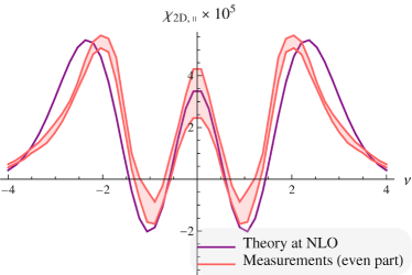
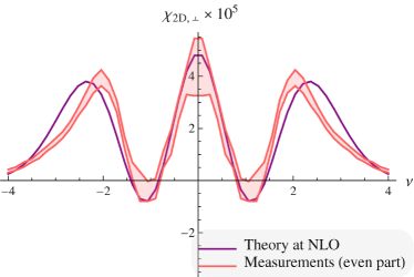
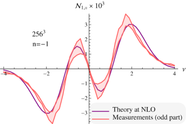
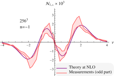
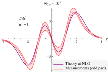
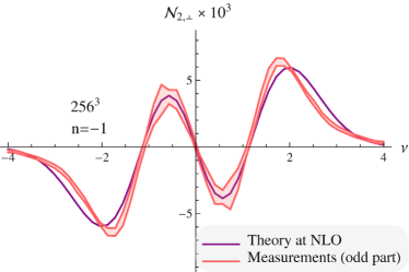
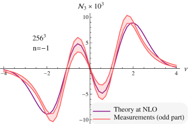
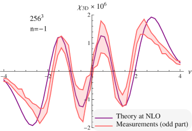
Figure 4: Gravity-induced NLO non-Gaussian corrections for the Minkowski functionals of a mildly non-linear 3D density field ($n=-1$, $\sigma=0.18$) in redshift space ($f=1$). Theoretical predictions are displayed with solid purple lines, measurements with shaded one sigma dispersion. Top left: 2D Euler characteristic in planes parallel to the LOS; top right: 2D Euler characteristic in planes perpendicular to the LOS; central top left: $\mathcal{N}_{1}$ (contour crossing) in planes parallel to the LOS; central top right: $\mathcal{N}_{1}$ in planes perpendicular to the LOS; central bottom left: $\mathcal{N}_{2}$ (length of iso-contour) in planes parallel to the LOS; central bottom right: $\mathcal{N}_{2}$ in planes perpendicular to the LOS; bottom left: $\mathcal{N}_{3}$ (area of iso-contour); bottom right: 3D Euler characteristic. Note that the predicted first order correction fits very well the odd part (resp. even for the 2D Euler characteristic) of the measured correction for intermediate contrast ($-1.5\lesssim\nu\lesssim 1.5$).

Figures 11 and 12 shows the dependence of the 2D Euler characteristic on $f_{nl}$ and $f$ following equations (43) and (44). As expected, the effect of redshift distortion is enhanced in 2D relative to 3D. This is expected since in 3D two dimensions remain isotropic. Figure 13 also shows the evolution of the 2D Euler characteristic as a function of $g_{\mathrm{{nl}}}$ and $f$. It demonstrates that this set of simulations is well fitted by the sum of the two contributions from $f_{\mathrm{{nl}}}$ and $g_{\mathrm{{nl}}}$.

For cosmological fields, Figure 4 compares the prediction of equation (43) for the ${\chi}_{\mathrm{2D}}$ statistics to scale invariant LSS simulations in planes parallel and perpendicular to the line of sight. Again, this figure shows a very good agreement between measurements and predictions at NLO for intermediate contrasts ($-1.5\lesssim\nu\lesssim 1.5$). There is a noticeable angle-dependence of the 2D Euler characteristic which suggests that the procedure described in the introduction of Section 4 is feasible. This angle dependence is also illustrated in Figure 5 where one can see how the prediction at next-to-leading order varies with the angle $\theta_{\cal S}$ between the line of sight and the 2D slice under consideration.

4.3 Other Minkowski functionals

4.3.1 Area of isodensity contours in 3D : ${\cal N}_{3}$

One of the Minkowski functionals is ${\cal N}_{3}(\nu)$, the area (per unit volume) of a 3D isosurface of the density field at level $\nu$. To compute this functional, it is sufficient to consider the JPDF of the field and its first derivatives

$$P(x,q_{\perp}^{2},x_{3})=\frac{1}{2\pi}\exp\left(-\frac{x^{2}}{2}-q_{\perp}^{2}-\frac{x_{3}^{2}}{2}\right)\left[1+\sum_{n=3}^{\infty}\sum_{\sigma_{n}}\frac{(-1)^{j}}{i!\,j!\,k!}\left\langle x^{i}q_{\perp}^{2j}x_{3}^{k}\right\rangle_{\textrm{GC}}H_{i}(x)L_{j}(q_{\perp}^{2})H_{k}(x_{3})\right].$$ (45)

From equation (2), the area of a 3D isosurface is

$${\cal N}_{3}(\nu)=\frac{1}{\sigma}\int\mathrm{d}q_{\perp}^{2}\mathrm{d}x_{3}P(\nu,q_{\perp}^{2},x_{3})\sqrt{\sigma_{1\perp}^{2}q_{\perp}^{2}+\sigma_{1\parallel}^{2}x_{3}^{2}}\,.$$ (46)

Computing the integrals, we express the results using the anisotropy parameter $\beta_{\sigma}=1-{\sigma_{1\perp}^{2}}/{2\sigma_{1\parallel}^{2}}$. At Gaussian order, expression (46) yields the result, consistent with Matsubara (1996),

$${\cal N}_{3}^{(0)}(\nu)=\frac{2}{\pi}\frac{\sigma_{1}}{\sqrt{3}\sigma}\frac{1-A(\beta_{\sigma})}{\sqrt{1-2\beta_{\sigma}/3}}e^{-\nu^{2}/2},\quad\textrm{with}\quad A(\beta_{\sigma})\equiv\frac{1}{2}\left(\vphantom{\frac{T}{\beta_{\sigma}}}\beta_{\sigma}-T\left(\beta_{\sigma}\right)+\beta_{\sigma}T\left(\beta_{\sigma}\right)\right),$$ (47)

where the function $T$ is defined as $T(\beta_{\sigma})=1/\sqrt{\beta_{\sigma}}\tanh^{-1}\left(\sqrt{\beta_{\sigma}}\right)-1$ for $\beta_{\sigma}\geq 0$ and $T(\beta_{\sigma})=1/\sqrt{|\beta_{\sigma}|}\tan^{-1}\left(\sqrt{|\beta_{\sigma}|}\right)-1$ for $\beta_{\sigma}<0$. Under this definition $A(\beta_{\sigma})$ describes a $\sim{\beta_{\sigma}}/{3}+\beta_{\sigma}^{2}/15+\ldots$ correction at small anisotropy $\beta_{\sigma}\to 0$. We see that in the Gaussian limit, the anisotropy has a very little effect on ${\cal N}_{3}$. The amplitude deviates from unity by less that 1% in the range $-1<\beta_{\sigma}<0.5$, as its series expansion $\propto 1-\beta_{\sigma}^{2}/90\ldots$ attests. Even at extreme anisotropies, it changes just to $\approx 0.92$ at $\beta_{\sigma}\to-\infty$ and $\approx 0.87$ at $\beta_{\sigma}=1$.

The computation of the $n=3$ term corresponding to the first non-Gaussian correction is also straightforward

$${\cal N}_{3}^{(1)}(\nu)={\cal N}_{3}^{(0)}(\nu)\Bigg{[}\frac{1}{3!}\left\langle x^{3}\right\rangle H_{3}(\nu)+\frac{1}{2}\left(\vphantom{\frac{T}{\beta_{\sigma}}}\left\langle xq_{\perp}^{2}\right\rangle+\frac{A(\beta_{\sigma})/\beta_{\sigma}}{1-A(\beta_{\sigma})}\left(\left\langle xx_{3}^{2}\right\rangle-\left\langle xq_{\perp}^{2}\right\rangle\right)\right)H_{1}(\nu)\Bigg{]}\,.$$ (48)

To first order in $\beta_{\sigma}$ (the anisotropy parameter), one gets the following explicit expression

$${\cal N}_{3}^{(1)}(\nu)=\frac{2e^{-\nu^{2}/2}\sigma_{1}}{\sqrt{3}\pi\sigma}\Bigg{[}1+\frac{1}{3!}\left\langle x^{3}\right\rangle H_{3}(\nu)+\frac{1}{2}\left(\frac{2}{3}\left\langle xq_{\perp}^{2}\right\rangle\left[1-\frac{4}{15}\beta_{\sigma}\right]+\frac{1}{3}\left\langle xx_{3}^{2}\right\rangle\left[1+\frac{8}{15}\beta_{\sigma}\right]\right)H_{1}(\nu)\Bigg{]}+{\cal O}(\beta_{\sigma}^{2})\,,$$ (49)

from which the isotropic limit of Gay et al. (2012) is readily recovered by setting $\beta_{\sigma}=0$ and $\left\langle xq_{\perp}^{2}\right\rangle=\left\langle xx_{3}^{2}\right\rangle=\left\langle xq^{2}\right\rangle$. We note that anisotropy effects in the ${\cal N}_{3}$ statistics are almost exclusively concentrated in the gradient terms $\propto H_{1}(\nu)$. This suggests, for example, that the recovery of the skewness $\langle x^{3}\rangle$ by fitting the $H_{3}(\nu)$ mode to ${\cal N}_{3}$ will be practically unaffected by redshift distortions. In contrast, one must focus on the $H_{1}(\nu)$ mode to measure anisotropic effects.

Figure 4 also compares the prediction of equation (49) for the ${\cal N}_{3}$ statistics to scale invariant LSS simulations ($256^{3}$, $n=-1$). Once again, in this mildly non-linear regime ($\sigma=0.18$ in real space), the prediction at NLO matches very well the measurement for intermediate contrasts ($-2\lesssim\nu\lesssim 2$) .

4.3.2 Length of isodensity contours in 2D planes : ${\cal N}_{2}$

Let us consider the length (per unit volume) of isodensity contours in 2D slices of the density field, ${\cal N}_{2}$. This functional is the 2D version of the Minkowski functional ${\cal N}_{3}$ for 3D field. Here the 2D slice is defined by the angle, $\theta_{\cal S}$, it makes with the $z$-axis and the statistical properties of the field depend on this angle. Again, let us start with the JPDF of the field and its gradient on a 2D plane. Using the same variables as in Section 4.2.2,

$$P(\tilde{x},{\tilde{x}_{1}},{\tilde{x}_{2}})=\frac{1}{(2\pi)^{3/2}}\exp\left(-\frac{\tilde{x}^{2}}{2}-\frac{{\tilde{x}_{1}}^{2}}{2}-\frac{{\tilde{x}_{2}}^{2}}{2}\right)\left[1+\sum_{n=3}^{\infty}\sum_{\sigma_{n}}\frac{1}{i!\,j!\,k!}\left\langle\tilde{x}^{i}{\tilde{x}_{1}}^{j}{\tilde{x}_{2}}^{k}\right\rangle_{\textrm{GC}}H_{i}(\tilde{x})H_{j}({\tilde{x}_{1}})H_{k}({\tilde{x}_{2}})\right]\;,$$ (50)

where $\sigma_{n}=\{(i,j,k)\in\mathbb{N}^{3}|i+2j+k=n\}$. From equation (2), the length of isodensity contours in 2D planes is now

$${\cal N}_{2}(\nu,\theta_{\cal S})=\frac{1}{\sigma}\int\mathrm{d}\tilde{x}_{1}\mathrm{d}\tilde{x}_{2}P(\nu,\tilde{x}_{1},\tilde{x}_{2})\sqrt{{\tilde{\sigma}_{1\perp}}^{2}\tilde{x}_{1}^{2}+{\tilde{\sigma}_{1\parallel}}^{2}\tilde{x}_{2}^{2}}\,.$$ (51)

We shall proceed similarly to the 3D case, defining the 2D anisotropy parameter $\tilde{\beta}_{\sigma}(\theta_{\cal S})$ which depends on the orientation of the plane

$$\tilde{\beta}_{\sigma}(\theta_{\cal S})\equiv 1-\frac{\tilde{\sigma}_{1\perp}^{2}}{\tilde{\sigma}_{1\parallel}^{2}}=\frac{\beta_{\sigma}\cos^{2}\theta_{\cal S}}{1-\beta_{\sigma}\sin^{2}\theta_{\cal S}}\,.$$ (52)

At Gaussian order, the evaluation of equation (51) yields, in agreement with Matsubara (1996)

$${\cal N}_{2}^{(0)}(\nu,\theta_{\cal S})=\frac{\tilde{\sigma}_{1\parallel}}{\pi\sigma}e^{-\nu^{2}/2}E\left(\tilde{\beta}_{\sigma}\right)=\frac{\sigma_{1\perp}}{\sqrt{2}\pi\sigma}e^{-\nu^{2}/2}\frac{E\left(\tilde{\beta}_{\sigma}\right)}{\sqrt{1-\tilde{\beta}_{\sigma}}}\,,$$ (53)

where $E$ is the complete elliptic integral of the second kind. The amplitude behaves as $E(\tilde{\beta}_{\sigma})/\sqrt{1-\tilde{\beta}_{\sigma}}\sim{\pi}/{2}+{\pi}\tilde{\beta}_{\sigma}/{8}$ at small $\tilde{\beta}_{\sigma}$ and is thus strongly dependent on the anisotropy parameter. This is distinct from the behaviour of ${\cal N}_{3}$.

Then, the first non-Gaussian correction (corresponding to $n=3$) reads

$${\cal N}_{2}^{(1)}(\nu,\theta_{\cal S})={\cal N}_{2}^{(0)}\Bigg{[}\!\frac{H_{3}(\nu)}{3!}\left\langle\tilde{x}^{3}\right\rangle\!+\!\frac{1}{2}H_{1}(\nu)\!\left(\!\left\langle\tilde{x}\tilde{x}_{2}^{2}\right\rangle\!+\!B(\tilde{\beta}_{\sigma})\left(\left\langle\tilde{x}\tilde{x}_{1}^{2}\right\rangle\!-\!\left\langle x\tilde{x}_{2}^{2}\right\rangle\right)\right)\!\Bigg{]},\,\textrm{with}\;B(\tilde{\beta}_{\sigma})=2(\tilde{\beta}_{\sigma}-1)\frac{\mathrm{d}\ln E(\tilde{\beta}_{\sigma})}{\mathrm{d}\tilde{\beta}_{\sigma}}\,.$$ (54)

Here on-plane cumulants are related to 3D ones by $\left\langle\tilde{x}{\tilde{x}_{1}}^{2}\right\rangle=\left\langle xq_{\perp}^{2}\right\rangle$ and $\left\langle\tilde{x}{\tilde{x}_{2}}^{2}\right\rangle=\left(1-\tilde{\beta}_{\sigma}/\beta_{\sigma}\right)\left\langle xq_{\perp}^{2}\right\rangle+\tilde{\beta}_{\sigma}/\beta_{\sigma}\left\langle xx_{3}^{2}\right\rangle$. In the small anisotropy limit, equation (54) becomes

$${\cal N}_{2}^{(1)}(\nu,\theta_{\cal S})=\frac{\sigma_{1\perp}}{2\sqrt{2}\sigma}e^{-\nu^{2}/2}\left(1+\frac{1}{4}\tilde{\beta}_{\sigma}\right)\Bigg{[}\frac{H_{3}(\nu)}{3!}\left\langle\tilde{x}^{3}\right\rangle+\frac{1}{4}H_{1}(\nu)\left(\left\langle\tilde{x}\tilde{x}_{1}^{2}\right\rangle+\left\langle\tilde{x}\tilde{x}_{2}^{2}\right\rangle-\frac{3}{8}\tilde{\beta}_{\sigma}\left(\left\langle\tilde{x}\tilde{x}_{1}^{2}\right\rangle-\left\langle\tilde{x}\tilde{x}_{2}^{2}\right\rangle\right)\right)\Bigg{]}+{\mathcal{O}}\left(\tilde{\beta}_{\sigma}^{2}\right)\,,$$ (55)

where the isotropic limit of Gay et al. (2012) is readily recognized at $\tilde{\beta}_{\sigma}=0$, $\left\langle\tilde{x}\tilde{x}_{1}^{2}\right\rangle=\left\langle\tilde{x}\tilde{x}_{2}^{2}\right\rangle=\left\langle xq^{2}\right\rangle$ and $\sigma_{1\perp}=\sqrt{2/3}\sigma_{1}$. We should stress that anisotropic effects in equation (55) are contained not only in the $\tilde{\beta}_{\sigma}$ factors, but in the deviation of cumulants from their isotropic values as well. Note that, with the 3D variables, equation (55) becomes

$${\cal N}_{2}^{(1)}(\nu,\theta_{\cal S})=\frac{\sigma_{1\perp}}{2\sqrt{2}\sigma}e^{-\nu^{2}/2}\left(1+\beta_{\sigma}\frac{\cos^{2}\theta_{\cal S}}{4}\right)\Bigg{[}\frac{H_{3}(\nu)}{3!}\left\langle x^{3}\right\rangle\\ +\frac{1}{4}H_{1}(\nu)\left(\left\langle xq_{\perp}^{2}\right\rangle+\left\langle xx_{3}^{2}\right\rangle+\left(\sin^{2}\theta_{\cal S}-\beta_{\sigma}\frac{\cos^{2}\theta_{\cal S}(3+5\sin^{2}\theta_{\cal S})}{8}\right)\left(\left\langle xq_{\perp}^{2}\right\rangle-\left\langle xx_{3}^{2}\right\rangle\right)\right)\Bigg{]}+{\mathcal{O}}\left(\beta_{\sigma}^{2}\right)\,.$$ (56)

The most interesting case for the ${\cal N}_{2}$ statistics is when the slice is passing through the observer, and, correspondingly, contains the line of sight. This is the case for 2D slices in observational catalogues such as SDSS. This setup corresponds to $\theta_{\cal S}=0$ and $\tilde{\beta}_{\sigma}=\beta_{\sigma}$. Indeed, the measurement of ${\cal N}_{2}$ in such slices gives direct access to the 3D anisotropy parameter $\beta_{\sigma}$, and, by extention, $\Omega_{m}^{0.6}/b$, even when full 3D data is not available. The study of 2D slices at different angles $\theta_{\cal S}$ is possible if the 3D cube of data is available and offers alternative way of analysing such cubes. Varying $\theta_{\cal S}$ allows to introduce functional dependence of statistics on the parameter, which gives additional access to $\tilde{\beta}_{\sigma}$ through variation of the amplitude of the statistics even when the normalization scale $\sigma_{1\perp}/\sigma$ is poorly determined.

Figure 4 compares the prediction of equation (54) for the ${\cal N}_{2}$ statistics to scale invariant LSS simulations in planes parallel and perpendicular to the line of sight. In both cases, measurements are well fitted by the prediction at the first non-Gaussian order for intermediate contrasts. One can easily notice that this statistics varies macroscopically with the angle $\theta_{\cal S}$. This dependence is also shown in Figure 5 for the NLO prediction. Indeed, Figure 5 displays the variation of the non-Gaussian contribution to the ${\cal N}_{2}$ statistics as a function of the orientation of the 2D slices relative to the LOS. Note that anisotropy affects the $H_{1}(\nu)$ harmonic of this dependence and can be detected by a linear fit to ${\cal N}_{2}^{(1)}(\nu,\theta_{\cal S})$ at different $\theta_{\cal S}$.

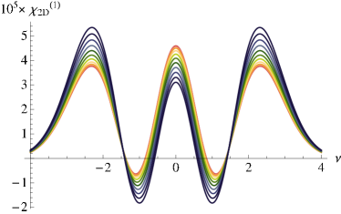
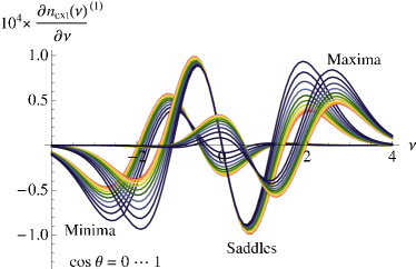
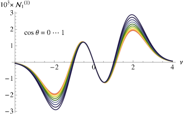
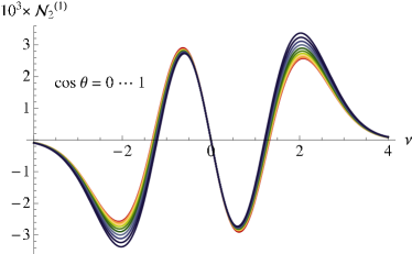
Figure 5: 2D Euler characteristic (top left panel), 2D extrema counts (top right panel), length of 2D iso-contour (bottom left panel) and contour crossing (bottom right panel) at first non-Gaussian order as a function of $\cos\theta_{\cal S}$ from 0 (red) to 1 (dark blue). Cumulants used in equations (43)-(54)-(60) are measured in a scale-invariant LSS simulation with $\sigma=0.18$ The prediction for 2D extrema statistics was obtained by numerical integration following Section 4.4. The noticeable dependence of these functionals on the angle $\theta_{\cal S}$ gives us a mean to measure $\beta=f/b_{1}$ as suggested in Section 5.5.

4.3.3 Contour crossings : ${\cal N}_{1}$

Contour-crossing statistics measures the average number of times a given line crosses the isocontours of a field, ${\cal N}_{1}$. It is closely related to the average area of the isocontours per unit volume, ${\cal N}_{3}$. It is equivalent to ${\cal N}_{3}$ when averaged over all possible orientations of the chosen line (indeed, the surface area per unit volume ${\cal N}_{3}$ can be understood as an average “hyperflux” of isosurfaces, i.e how many time per unit length they cross a random line), but has distinct dependence on line orientation if the field is anisotropic. A special advantage of ${\cal N}_{1}$ is that it can be applied when only a “pencil beam” data is available, as for example in $Ly_{\alpha}$ lines, although in this case one is limited to use only the line-of-sight direction of the field. In general, the behaviour of ${\cal N}_{1}$ along lines with arbitrary orientation relative to the LOS contains additional information.

To compute contour-crossing statistics, we assume (without loss of generality) that the line intersecting the field lies in the ($\mathbf{u_{1}},\mathbf{u_{3}}$) plane with a direction defined by the unit vector $\hat{l}=(\sin\theta_{\cal L},0,\cos\theta_{\cal L})$. Then the mean number of intersections between a line $(\cal L)$ and the isodensity contours is simply the average of the field gradient projection $|\nabla x\cdot\hat{l}|=\left|\sigma_{1\perp}x_{1}\sin\theta_{L}/\sqrt{2}+\sigma_{1\parallel}x_{3}\cos\theta_{L}\right|$. In contrast to the 2D statistics case, we shall not introduce tilde variables on the line, and write the statistics immediately in terms of the 3D variables. Starting from the JPDF of the field and two components of its first derivatives

$$P(x,x_{1},x_{3})=\frac{1}{(2\pi)^{3/2}}\exp\left(-\frac{x^{2}}{2}-\frac{x_{1}^{2}}{2}-\frac{x_{3}^{2}}{2}\right)\left[1+\sum_{n=3}^{\infty}\sum_{i,j,k=0}^{i+j+k=n}\frac{1}{i!\,j!\,k!}\left\langle x^{i}x_{1}^{j}x_{3}^{k}\right\rangle_{\textrm{GC}}H_{i}(x)H_{j}(x_{1})H_{k}(x_{3})\right]\,,$$ (57)

from equation (2), we write

$${\cal N}_{1}(\nu,\theta_{\cal L})=\frac{1}{\sigma}\int\mathrm{d}x_{1}\mathrm{d}x_{3}P(\nu,x_{1},x_{3})\left|\frac{\sigma_{1\perp}}{\sqrt{2}}x_{1}\sin\theta_{\cal L}+\sigma_{1\parallel}x_{3}\cos\theta_{\cal L}\right|.$$ (58)

At Gaussian order, using again $\beta_{\sigma}=1-{\sigma_{1\perp}^{2}}/{2\sigma_{1\parallel}^{2}}$, we find, in agreement with Matsubara (1996):

$${\cal N}_{1}^{(0)}(\nu,\theta_{\cal L})=\frac{\sigma_{1\parallel}}{\pi\sigma}e^{-\nu^{2}/2}\sqrt{1-\beta_{\sigma}\sin^{2}\theta_{L}},$$ (59)

Focusing on the next order term ($n=3$) and using the relationships $\langle xx_{1}x_{3}\rangle=\langle x^{2}x_{i}\rangle=0$, one gets

$${\cal N}_{1}^{(1)}(\nu,\theta_{\cal L})={\cal N}_{1}^{(0)}(\theta_{\cal L},\nu)\Bigg{[}\frac{1}{3!}\left\langle x^{3}\right\rangle H_{3}(\nu)+\frac{1}{2}H_{1}(\nu)\left(\left\langle xq_{\perp}^{2}\right\rangle+\frac{\cos^{2}\theta_{\cal L}}{1-\beta_{\sigma}\sin^{2}\theta_{\cal L}}\left(\left\langle xx_{3}^{2}\right\rangle-\left\langle xq_{\perp}^{2}\right\rangle\right)\right)\Bigg{]}.$$ (60)

In the isotropic limit where $\beta_{\sigma}=0$ and $\left\langle xq_{\perp}^{2}\right\rangle=\left\langle xx_{3}^{2}\right\rangle=\left\langle xq^{2}\right\rangle$, equations (59) and (60) together becomes

$${\cal N}_{1}^{\textrm{iso}}(\nu)=\frac{e^{-\nu^{2}/2}\sigma_{1}}{\sqrt{3}\pi\sigma}\Bigg{[}1+\frac{1}{3!}H_{3}(\nu)\left\langle x^{3}\right\rangle+\frac{1}{2}H_{1}(\nu)\left\langle xq^{2}\right\rangle+{\cal O}(\sigma^{2})\Bigg{]}.$$ (61)

Figure 4 compares the prediction of equation (60) for the ${\cal N}_{1}$ statistics to scale invariant LSS simulations in planes parallel and perpendicular to the line of sight. The agreement between the prediction at NLO and measurements is very good for contrasts in the range $-2\lesssim\nu\lesssim 2$. The tails of the distribution are more sensitive to higher-order terms in the GC expansion. Planes parallel and perpendicular to the line of sight give rise to a noticeable difference in the first order correction for the contour crossing statistics. Figure 5 also displays the variation of ${\cal N}_{1}$ as a function of the orientation of the 2D slices relative to the LOS.

4.4 Extrema counts

Extrema counts are given by averaging the absolute value of the determinant of the Hessian ($I_{3}$ and $I_{2}$ in 3D and 2D respectively) under the condition of zero gradient over the range of Hessian eigenvalues space that maintains the correspondent signature of the sorted eigenvalues, namely, in 3D, $\lambda_{1}>\lambda_{2}>\lambda_{3}>0$ for minima, $\lambda_{1}>\lambda_{2}>0>\lambda_{3}$ for pancake-like saddle points, $\lambda_{1}>0>\lambda_{2}>\lambda_{3}$ for filamentary saddle points and $0>\lambda_{1}>\lambda_{2}>\lambda_{3}$ for maxima. The integral to perform is similar to that for the Euler characterstic, e.g. equation (31) in 3D

$$n_{\mathrm{ext,3D}}=\frac{1}{\sigma_{1\perp}^{2}\sigma_{1\parallel}}\int_{\rm fixed\leavevmode\nobreak\ \lambda_{i}\leavevmode\nobreak\ signs}\mathrm{d}x\,\mathrm{d}\zeta\,\mathrm{d}J_{2\perp}\mathrm{d}\xi\,\mathrm{d}Q^{2}\mathrm{d}\Upsilon P_{\textrm{ext}}(x,\zeta,J_{2\perp}\xi,Q^{2},\Upsilon)|I_{3}|\,,$$ (62)

the principal difference being in the limits of integration. The signature of the eigenvalues set changes where $I_{3}$ changes sign. In terms of the invariant variables, $I_{3}$ is given by equation (32). The equation $I_{3}=0$ that follows from equation (32) is more instructive if one writes it in the form that uses the full 3D Hessian rotation invariants, $J_{1}$, $J_{2}$, $J_{3}$

$$J_{1}^{3}-3J_{2}\left(y,J_{2\perp},Q^{2},\Upsilon\right)J_{1}-2J_{3}\left(y,J_{2\perp},Q^{2},\Upsilon\right)=0\,,$$ (63)

where $J_{1}=J_{1\perp}+x_{33}$, $J_{2}=y^{2}+3J_{2\perp}/4+3Q^{2}$, $J_{3}=-y^{3}+9y\left({J_{2\perp}}-2Q^{2}\right)/4+{27}\Upsilon/{4}$ with $y=J_{1\perp}/2-x_{33}$ where for this equation only, for the sake of simplicity, variables are not rescaled by their variance. It can be shown that for any values of $Q^{2},J_{2\perp},\Upsilon$ and $y$ in their unrestricted allowed range there exist three real roots for this cubic polynomial in $J_{1}$ that split the integration over $J_{1}$ in four regions corresponding to different extrema types. No restriction on other variables arise besides choosing the threshold of the field value for differential counts.

The integral required to predict extrema counts in 2D is given by equation (39) (where $P_{2\textrm{D}}(\tilde{x},\tilde{x}_{1},\tilde{x}_{2},\tilde{\zeta},\tilde{\xi},\tilde{x}_{12})$ is defined in equation (24)) and is carried in terms of the field variables, $\tilde{x}_{11},\tilde{x}_{12},\tilde{x}_{22}$, subject to constraints on the signs of the eigenvalues of the Hessian.

Extrema counts in anisotropic 2 and 3D spaces do not have closed form expressions (indeed, differential 3D extrema counts do not lead to analytic results even in the Gaussian limit). Therefore we shall not present here intermediate expressions for formal expansion, and instead will be performing the averaging numerically. Recall however, that in the rare event limit, $\nu\gg 1$ or $\nu\ll-1$, $n_{\mathrm{max/min}}(\nu)\simeq\chi(\nu)$, so that in this limit, equations (40) and (130) provide an all-order expansion of the extrema counts in redshift space in 2 and 3D respectively.

We can also establish the following general symmetry relations between extrema counts of different types, valid in a space of arbitrary dimension $N$. Let us label the extrema type by its signature $S$ which is the sum of the signs of the eigenvalues of the Hessian that define its type. This way, $S=N$ for minima ($N$ positive eigenvalues), $S=-N$ for maxima ($N$ negative eigenvalues) and $S$ changes with a step of two between $2-N$ to $N-2$ for saddle points of different types. Then, if we denote by $\partial_{\nu}n_{\textrm{S}}^{(n)}$ the contribution to the differential number count of extrema of type $S$ of order $n$ (where $n=2$ corresponds to the Gaussian term), the following holds

$$\partial_{\nu}n_{\textrm{S}}^{(n)}(\nu)=(-1)^{n}\partial_{\nu}n_{\textrm{-S}}^{(n)}(-\nu)\leavevmode\nobreak\ \leavevmode\nobreak\ .$$ (64)

These relations allow us to predict the expected behaviour of extrema counts of type $S$ from the measurements of their “conjugate” type $-S$. In particular, the minima counts Gram-Charlier terms are equal to the reflected ($\nu\to-\nu$) maxima counts for even $n$ (including the Gaussian term), and to minus the reflected maxima counts for odd $n$ (including the first non-Gaussian correction). The same relation holds between the “pancake-like” ($S=1$) and the “filament-like” ($S=-1$) saddle points in 3D.

Figure 14 illustrates the corresponding extrema distribution for a set of anisotropic fields (Gaussian and first order non-Gaussian correction) in 2D and 3D. A comparison with extrema counts measured from random realisations of the fields (scale invariant $n=-1$ field sampled on $4096^{2}$ pixels) is also presented there. Figure 5 demonstrates the angular dependence of the predicted extrema counts at NLO in a scale-invariant LSS simulation ($n=-1$, $\sigma=0.18$ in real space).

4.5 Invariance of critical sets

4.5.1 Summary of the Minkowski functionals as functions of $\nu_{f}$

To put the mathematical results derived in Sections 4.2.1-4.3.3 on a practical footing in cosmology, let us collect them expressed as functions of the observable threshold variable $\nu_{f}$. The $\nu\rightarrow\nu_{f}$ remapping is astrophysically motivated by the fact that typically, the amplitude of the field is not known, as it may depend on e.g. the bias factor, whereas $\nu_{f}$ can be measured. The value of $\nu_{f}$ is obtained by inverting equation (29) for the filling factor, $f_{V}$, and using it instead of the difficult-to-determine $\nu$, to effectively “Gaussianize” the PDF of the field. Indeed, when the transformation $\nu\to\nu_{f}$ in equation (30) is applied to perturbative results, the most oscillatory $\nu$ modes, that are proportional solely to the cumulants of the field, are eliminated.

In analogy with the skewness parameter $S_{3}=\langle x^{3}\rangle/\sigma$, we introduce two other scaled cumulants that involve the derivatives of the field. For isotropic fields, they are $T_{3}=\langle xq^{2}\rangle/\sigma$ and $U_{3}=-\langle J_{1}q^{2}\rangle/(\gamma\sigma)$. For anisotropic fields, we use their partial versions $T_{3\perp}=\langle xq_{\perp}^{2}\rangle/\sigma$, $T_{3\parallel}=\langle xq_{\parallel}^{2}\rangle/\sigma$ and $U_{3\perp}=-\langle J_{1\perp}q_{\perp}^{2}\rangle/(\gamma_{\perp}\sigma)$, $U_{3\parallel}=-\langle J_{1\perp}q_{\parallel}^{2}\rangle/(\gamma_{\perp}\sigma)$. In the isotropic limit these partial contributions are summed according to the following rules $T_{3}=\frac{1}{3}\left(2T_{3\perp}+T_{3\parallel}\right)$ and $U_{3}=\frac{4}{9}\left(U_{3\perp}+U_{3\parallel}\right)$ . It is then straightforward to rewrite our statistics, e.g. the 3D Euler characteristic, as a function of $\nu_{f}$

$$\chi_{\mathrm{{3D}}}(\nu_{f})=\frac{\sigma_{1\parallel}\sigma_{1\perp}^{2}}{\sigma^{3}}\frac{e^{-\nu_{f}^{2}/2}}{8\pi^{2}}\left(H_{2}(\nu_{f})+\sigma\left[\left(T_{3\perp}+\frac{1}{2}T_{3\parallel}-S_{3}\right)H_{3}(\nu_{f})+\left(U_{3\perp}+U_{3\parallel}-S_{3}\right)H_{1}(\nu_{f})\right]+\cdots\right)\,.$$ (65)

Note that in contrast to the isotropic case, in redshift space the coefficient of $H_{1}$, $\tilde{S}^{(1)}_{z}=U_{3\perp}+U_{3\parallel}-S_{3}$, is non-zero for scale-invariant power spectra. For the other statistics, we get:
the area of 3D isocontours

$${\cal N}_{3}(\nu_{f})={\cal N}_{3}^{(0)}(\nu_{f})\left(1+\sigma H_{1}(\nu_{f})\left[\frac{1}{2}\vphantom{\frac{T}{\beta_{\sigma}}}\left(1-\frac{A(\beta_{\sigma})/\beta_{\sigma}}{1-A(\beta_{\sigma})}\right)T_{3\perp}+\frac{1}{2}\left(\frac{A(\beta_{\sigma})/\beta_{\sigma}}{1-A(\beta_{\sigma})}\right)T_{3\parallel}-S_{3}\right]+\cdots\right)\,,$$ (66)

the 2D Euler characteristic

$$\chi_{2\textrm{D}}(\nu_{f},\theta_{\cal S})=\frac{\tilde{\sigma}_{1\perp}\tilde{\sigma}_{1\parallel}}{\sigma^{2}}\frac{e^{-\nu_{f}^{2}/2}}{(2\pi)^{3/2}}\left(H_{1}\left(\nu_{f}\right)+\sigma\left[H_{2}(\nu_{f})\left(\frac{1}{2}\frac{\left\langle\tilde{x}\left[{\tilde{x}_{1}}^{2}+{\tilde{x}_{2}}^{2}\right]\right\rangle}{\sigma}-S_{3}\right)+\left(-\frac{1}{2{\tilde{\gamma}_{\perp}}}\frac{\left\langle{\tilde{x}_{11}}{\tilde{x}_{2}}^{2}\right\rangle}{\sigma}-S_{3}\right)\right]+\cdots\right)\,,$$ (67)

the length of 2D isocontours

$${\cal N}_{2}(\nu_{f},\theta_{\cal S})={\cal N}_{2}^{(0)}(\nu_{f})\left(1+\sigma H_{1}(\nu_{f})\left[\frac{1}{2}\frac{\left\langle\tilde{x}\tilde{x}_{1}^{2}\right\rangle}{\sigma}B(\tilde{\beta}_{\sigma})+\frac{1}{2}\frac{\left\langle\tilde{x}\tilde{x}_{2}^{2}\right\rangle}{\sigma}\left(1-B(\tilde{\beta}_{\sigma})\right)-S_{3}\right]+\cdots\right)\,,$$ (68)

and the frequency of contour crossings

$${\cal N}_{1}(\nu_{f},\theta_{\cal L})={\cal N}_{1}^{(0)}(\nu_{f})\left(1+\sigma H_{1}(\nu_{f})\left[\frac{1}{2}\frac{(1-\beta_{\sigma})\sin^{2}\theta_{\cal L}T_{3\perp}+\cos^{2}\theta_{\cal L}T_{3\parallel}}{1-\beta_{\sigma}\sin^{2}\theta_{\cal L}}-S_{3}\right]+\cdots\right)\,.$$ (69)

Note that $\left\langle\tilde{x}\tilde{x}_{1}^{2}\right\rangle$, $\left\langle\tilde{x}\tilde{x}_{1}^{2}\right\rangle$ and $\left\langle\tilde{x}_{11}\tilde{x}_{2}^{2}\right\rangle$ are functions of $\theta_{\cal S/\cal L}$, $T_{3\perp}$, $T_{3\parallel}$, $U_{3\perp}$ and $U_{3\parallel}$. Using $\nu_{f}$ as a threshold variable makes explicit the invariance of Minkowski functionals and extrema statistics under monotonic transformation of the field. Indeed, since the filling factor $f_{V}$ is one of the Minkowski functionals itself, $\nu_{f}$ is strictly unchanged under monotonic transformation. Thus the other statistics, described by functions of $\nu_{f}$, are invariant.

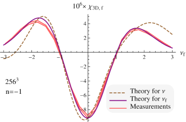
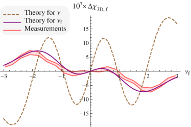
Figure 6: Left panel : 3D Euler characteristic as a function of $\nu_{f}$ in 19 scale-invariant LSS simulation ($n=-1,256^{3},\sigma=0.18$). Prediction to first order in non-Gaussianity is displayed in solid purple line. The displayed error is the error on the median of the measurements (red shaded area). For comparison, the 3D Euler characteristic as a function of $\nu$ is displayed in dashed brown line. Right panel: same as left panel for the first non-Gaussian correction only compared to the odd part of the measurements (including the first order correction). In this mildly non-linear regime, the agreement between measurements and theory at leading and next-to-leading order is very good. Note how the use of $\nu_{f}$ instead of $\nu$ “gaussianizes” the Euler characteristic.

Figure 6 reproduces the 3D Euler characteristic of Figure 2 but as a function of the filling factor threshold, $\nu_{f}$, defined in Section 4.1. Agreement between prediction truncated at NLO and measurements is very good for contrasts $\nu\lower 2.15277pt\hbox{$\;\buildrel>\over{\sim}\;$}-1.5$. The effect of using $\nu_{f}$ is to gaussianize the PDF as seen on Figure 6 : denser regions are brought to the center whereas wider regions are pushed to the outside.

4.5.2 Formal invariance of Minkowski functionals w.r.t. monotonic transformation

From Section 2, it is straightforward to see that any Minkowski functional as well as extrema counts are invariant under a local monotonic transformation. This property should also be encoded in the Gram-Charlier expansions of these Minkowski functionals given in Section 4.5.1. Indeed the combinations of cumulants which appear at first order in the Gram-Charlier expansion are invariant under local monotonic transformation taken to the same first order in $\sigma$. Let us illustrate this on the 3D Euler characteristic (given that the same proof can be developed for any Minkowski functionals). Following Matsubara (2003), let us henceforth study how cumulants evolve under the transformation: $y\rightarrow b\,x+{b_{2}}/{2}\left(x^{2}-\left\langle x^{2}\right\rangle\right)$, which represents the local representation of any analytic function of the density field when Taylor expanded. Let us first show how $\left\langle x^{3}\right\rangle$ evolve under such transformation

$$\left\langle y^{3}\right\rangle = b^{3}\left\langle x^{3}\right\rangle+\frac{3}{2}b^{2}b_{2}\left(\left\langle x^{4}\right\rangle-\left\langle x^{2}\right\rangle^{2}\right)+\frac{3}{4}b\,b_{2}^{2}\left(\left\langle x^{5}\right\rangle-2\left\langle x^{3}\right\rangle\left\langle x^{2}\right\rangle\right)\,,$$ (70)

$$= b^{3}\left\langle x^{3}\right\rangle_{c}+\frac{3}{2}b^{2}b_{2}\left(\left\langle x^{4}\right\rangle_{c}+2\left\langle x^{2}\right\rangle_{c}^{2}\right)+\frac{3}{4}b\,b_{2}^{2}\left(\left\langle x^{5}\right\rangle_{c}+8\left\langle x^{3}\right\rangle_{c}\left\langle x^{2}\right\rangle_{c}\right)\,.$$

Selecting only the first order term in the PT expansion, the classical expression for the skewness follows from Equation (70)

$$\left\langle y^{3}\right\rangle=b^{3}\left\langle x^{3}\right\rangle_{c}+3b^{2}b_{2}\left\langle x^{2}\right\rangle_{c}^{2}+\textrm{higher order terms }\,.$$ (71)

The same construction for other moments and cumulants leads to the following relationships

$$\left\langle y^{2}\right\rangle =b^{2}\left\langle x^{2}\right\rangle+\textrm{higher order terms }\,,$$ (72a)

$$\left\langle\nabla_{\perp}y\cdot\nabla_{\perp}y\right\rangle =b^{2}\left\langle\nabla_{\perp}x\cdot\nabla_{\perp}x\right\rangle+\textrm{higher order terms }\,,$$ (72b)

$$\left\langle\nabla_{\parallel}y\cdot\nabla_{\parallel}y\right\rangle =b^{2}\left\langle\nabla_{\parallel}x\cdot\nabla_{\parallel}x\right\rangle+\textrm{higher order terms }\,,$$ (72c)

$$\left\langle y(\nabla_{\perp}y)^{2}\right\rangle =b^{3}\left\langle x(\nabla_{\perp}x)^{2}\right\rangle+2b^{2}b_{2}\left\langle x^{2}\right\rangle\left\langle(\nabla_{\perp}x)^{2}\right\rangle+\textrm{higher order terms }\,,$$ (72d)

$$\left\langle y(\nabla_{\parallel}y)^{2}\right\rangle =b^{3}\left\langle x(\nabla_{\parallel}x)^{2}\right\rangle+2b^{2}b_{2}\left\langle x^{2}\right\rangle\left\langle(\nabla_{\parallel}x)^{2}\right\rangle+\textrm{higher order terms }\,,$$ (72e)

$$\left\langle(\nabla_{\perp}y\cdot\nabla_{\perp}y)\Delta_{\perp}y\right\rangle =b^{3}\left\langle(\nabla_{\perp}x\cdot\nabla_{\perp}x)\Delta_{\perp}y\right\rangle-b^{2}b_{2}\left\langle(\nabla_{\perp}x)^{2}\right\rangle^{2}+\textrm{higher order terms }\,,$$ (72f)

$$\left\langle(\nabla_{\parallel}y\cdot\nabla_{\parallel}y)\Delta_{\perp}y\right\rangle =b^{3}\left\langle(\nabla_{\parallel}x\cdot\nabla_{\parallel}x)\Delta_{\perp}y\right\rangle-2b^{2}b_{2}\left\langle(\nabla_{\perp}x)^{2}\right\rangle\left\langle(\nabla_{\parallel}x)^{2}\right\rangle+\textrm{higher order terms }\,,$$ (72g)

so that for $b\neq 0$ at leading order

$$\tilde{S}^{(1)}_{\chi_{\textrm{3D}},z}(y) \equiv \frac{1}{\left\langle y^{2}\right\rangle}\left(\frac{\left\langle y(\nabla_{\perp}y)^{2}\right\rangle}{\left\langle(\nabla_{\perp}y)^{2}\right\rangle}+\frac{\left\langle y(\nabla_{\parallel}y)^{2}\right\rangle}{2\left\langle(\nabla_{\parallel}y)^{2}\right\rangle}-\frac{\left\langle y^{3}\right\rangle}{\left\langle y^{2}\right\rangle}\right)=\tilde{S}^{(1)}_{\chi_{\textrm{3D}},z}(x)\,,$$ (73)

$$\tilde{S}^{(-1)}_{\chi_{\textrm{3D}},z}(y) \equiv \frac{1}{\left\langle y^{2}\right\rangle}\left(-\frac{\left\langle\Delta_{\perp}y(\nabla_{\perp}y)^{2}\right\rangle}{\left\langle(\nabla_{\perp}y)^{2}\right\rangle}-\frac{\left\langle\Delta_{\perp}y(\nabla_{\parallel}y)^{2}\right\rangle}{\left\langle(\nabla_{\parallel}y)^{2}\right\rangle}-\frac{\left\langle y^{3}\right\rangle}{\left\langle y^{2}\right\rangle}\right)=\tilde{S}^{(-1)}_{\chi_{\textrm{3D}},z}(x)\,,$$ (74)

where we denote $\tilde{S}^{(i)}_{\chi_{\textrm{3D}},z}$ the coefficients in front of the Hermite polynomials in equation (65) (see also equation (25)). This shows that the combinations of cumulants in front of the Hermite polynomials are invariant under local monotonic transformation and so are the Minkowski functionals. In particular, it demonstrates formally why if the bias is local and monotonic, the Minkowski functionals are bias-independent.

5 Application to large-scale structure in redshift space

In the context of cosmology, it is of interest to understand what kind of constraints on the cosmological parameters can be drawn from the prediction of critical sets in redshift space. Redshift space distortion can be viewed as a nuisance, but in fact potentially opens new prospects given the broken symmetry induced by the kinematics.

5.1 Estimating cumulants of the field

Table 1 summarizes the cubic cumulants that determine the Minkowski functionals studied in this paper to first non-Gaussian order. In turn, the combinations of these cumulants is what can be measured by fitting the correspondent functionals with low-order Hermite modes.

$$\begin{array}[]{c|c|c|c|c}&H_{0}&H_{1}&H_{2}&H_{3}\\ \hline\cr\chi_{\mathrm{{3D},f}}&-&\left\langle J_{1\perp}{q^{2}_{\perp}}\right\rangle,\left\langle J_{1\perp}x_{3}^{2}\right\rangle,\left\langle x^{3}\right\rangle&-&\left\langle xq_{\perp}^{2}\right\rangle,\left\langle xx_{3}^{2}\right\rangle,\left\langle x^{3}\right\rangle\\ \chi_{\mathrm{{2D},f}}&\left\langle J_{1\perp}{q^{2}_{\perp}}\right\rangle,\left\langle J_{1\perp}x_{3}^{2}\right\rangle,\left\langle x^{3}\right\rangle&-&\left\langle xq_{\perp}^{2}\right\rangle,\left\langle xx_{3}^{2}\right\rangle,\left\langle x^{3}\right\rangle&-\\ {\cal N}_{3,f}&-&\left\langle xq_{\perp}^{2}\right\rangle,\left\langle xx_{3}^{2}\right\rangle,\left\langle x^{3}\right\rangle&-&-\\ {\cal N}_{2,f}&-&\left\langle xq_{\perp}^{2}\right\rangle,\left\langle xx_{3}^{2}\right\rangle,\left\langle x^{3}\right\rangle&-&-\\ {\cal N}_{1,f}&-&\left\langle xq_{\perp}^{2}\right\rangle,\left\langle xx_{3}^{2}\right\rangle,\left\langle x^{3}\right\rangle&-&-\end{array}$$

Table 1: The cubic cumulants that determine the Minkowski functionals studied in this paper to first non-Gaussian order.

Two main group of cumulants that Minkowski functionals (to first order) give access to are $\left\langle xq_{\perp}^{2}\right\rangle,\left\langle xx_{3}^{2}\right\rangle$, which relate the field to its gradient, and $\left\langle J_{1\perp}{q^{2}_{\perp}}\right\rangle,\left\langle J_{1\perp}x_{3}^{2}\right\rangle$ which relate the gradient to the Hessian. Note that $\langle x^{3}\rangle$ is not accessible as the amplitude of an independent Hermite mode if Minkowski functionals are studied as functions of the filling factor threshold $\nu_{f}$. Rather it offsets the modes defined by the other two groups of cumulants. Redshift space analysis is in principle capable of mining more information than real space analysis. Indeed, in redshift space there is a qualitative difference between cumulants that involve the LOS direction and those that involve directions orthogonal to the LOS in the plane of the sky. These differences encode information about velocities, and reflect the mechanism of how these velocities originated. In principle, estimating the anisotropic part of such cumulants can be used to test the theory of gravity in the context of large-scale structures perturbation theory. 3D geometrical statistics, such as $\chi_{\mathrm{3D}}$ and ${\cal N}_{3}$ do not allow by themselves to determine separately the LOS and sky cumulants. To separate anisotropic contributions one must analyse slices of 3D volume at different angles $\theta_{\cal S}$ to the LOS. For instance, measuring the length of the isocontours, ${\cal N}_{2}$, (with possible cross-check from $\chi_{\mathrm{2D}}$) yields a separate handle on $\left\langle xq_{\perp}^{2}\right\rangle$ and $\left\langle xx_{3}^{2}\right\rangle$, while the additional analysis of the 2D Euler characteristic $\chi_{\mathrm{2D}}(\nu_{f})$, as a function of $\theta_{\cal S}$ (via the baseline offset $\propto H_{0}$, see figure 5) allows us to measure $\left\langle J_{1\perp}{q^{2}_{\perp}}\right\rangle$ and $\left\langle J_{1\perp}{x_{3}^{2}}\right\rangle$. This procedure is further discussed in Section 5.5 below.

5.2 Which modes of the bispectrum are geometrical statistics probing?

This paper is concerned with geometric probes operating in configuration space. On the other hand, a fair amount of theoretical predictions (such as PT) for the growth of structure are best described in Fourier space. It is therefore of interest to relate the two and characterize which feature of the multi-spectra these probes constrain. For instance, it is straightforward to show via Fourier transform that the third order cumulant, $\left\langle x^{3}\right\rangle$, can be expressed as a double sum over the anisotropic bispectrum, $B_{z}(k_{1},k_{2},k_{3})$ via

$$\left\langle x^{3}\right\rangle=\displaystyle\frac{1}{\sigma^{3}}\int\frac{\mathrm{d}^{3}k_{1}}{(2\pi)^{3}}\frac{\mathrm{d}^{3}k_{2}}{(2\pi)^{3}}B(k_{1},k_{2},|\mathbf{k_{1}+k_{2}}|)\,.$$

Measuring $\left\langle x^{3}\right\rangle$ amounts to constraining the monopole of the bispectrum. Similarly, other geometric cumulants involve different weights (see Table 2), while higher order cumulants will involve $k$ integrals of multi-spectra. For instance, the Euler characteristic to all order given in equation (132), involves $n^{\rm th}=i+2j+2m$ moments, $\left\langle x^{i}q^{2j}_{\perp}x_{3}^{2m}\right\rangle$ which can be re-expressed via the $n^{\rm th}$ order multi-spectrum, $B^{n}_{z}(k_{1},\cdots,k_{n-1},|\mathbf{k}_{1}+\cdots\mathbf{k}_{n-1}|)$ as

$$\left\langle x^{i}q^{2j}_{\perp}x_{3}^{2m}\right\rangle=\displaystyle\frac{1}{\sigma^{i}\sigma^{2j}_{1\perp}\sigma^{2m}_{1\parallel}}\int\frac{\mathrm{d}^{3}k_{1}}{(2\pi)^{3}}\cdots\frac{\mathrm{d}^{3}k_{n-1}}{(2\pi)^{3}}B^{n}_{z}(k_{1},\cdots,k_{n-1},|\mathbf{k}_{1}+\cdots\mathbf{k}_{n-1}|)\prod_{j_{1}\leq j}|\mathbf{k}_{j_{1}\perp}|^{2}\prod_{j<m_{1}\leq m+j}|\mathbf{k}_{m_{1}\parallel}|^{2}\,.$$

Let us first show explicitly how the first order corrections of the 3D Euler characteristic can be re-expressed in terms of the underlying bispectrum in redshift space, $B_{z}$. Equation (65) shows that it only depends at first order in non-Gaussianity on two numbers (the coefficients in front of the two Hermite polynomials): $\sigma\tilde{S}^{(1)}_{\chi_{\textrm{3D}},z}=\left\langle x(q_{\perp}^{2}+x_{3}^{2}/2)\right\rangle-\left\langle x^{3}\right\rangle$ and $\sigma\tilde{S}^{(-1)}_{\chi_{\textrm{3D}},z}=-\left\langle J_{1\perp}(q_{\perp}^{2}+x_{3}^{2})\right\rangle/\gamma_{\perp}-\left\langle x^{3}\right\rangle$. These quantities can in turn be expressed as special combinations of the underlying bispectrum using Table 2

$$\tilde{S}^{(1)}_{\chi_{\textrm{3D}},z} = \frac{1}{\sigma^{4}}\int\frac{\mathrm{d}^{3}k_{1}}{(2\pi)^{3}}\frac{\mathrm{d}^{3}k_{2}}{(2\pi)^{3}}\left(\frac{\sigma^{2}|\mathbf{k_{1\perp}+k_{2\perp}}|^{2}}{2\sigma_{1\perp}^{2}}+\frac{\sigma^{2}|\mathbf{k_{1\parallel}+k_{2\parallel}}|^{2}}{2\sigma_{1\parallel}^{2}}-1\right)B_{z}(k_{1},k_{2},|\mathbf{k_{1}+k_{2}}|)\,,$$ (75)

$$\tilde{S}^{(-1)}_{\chi_{\textrm{3D}},z} = -\frac{1}{\sigma^{4}}\int\frac{\mathrm{d}^{3}k_{1}}{(2\pi)^{3}}\frac{\mathrm{d}^{3}k_{2}}{(2\pi)^{3}}\left(\frac{\sigma^{4}|\mathbf{k_{1\perp}+k_{2\perp}}|^{2}(\mathbf{k}_{1\perp}\cdot\mathbf{k}_{2\perp})}{\sigma_{1\perp}^{4}}+\frac{\sigma^{4}|\mathbf{k_{1\perp}+k_{2\perp}}|^{2}(\mathbf{k}_{1\parallel}\cdot\mathbf{k}_{2\parallel})}{\sigma_{1\perp}^{2}\sigma_{1\parallel}^{2}}+1\right)B_{z}(k_{1},k_{2},|\mathbf{k_{1}+k_{2}}|)\,.$$ (76)

The parenthesis in equations (75)-(76) define “projectors” for the bispectrum, $(\tilde{S}^{(1)}_{\chi_{\textrm{3D}},z})_{B}$ and $(\tilde{S}^{(-1)}_{\chi_{\textrm{3D}},z})_{B}$, so that

$$\tilde{S}^{(i)}_{\chi_{\textrm{3D}},z}=\frac{1}{\sigma^{4}}\int\frac{\mathrm{d}^{3}k_{1}}{(2\pi)^{3}}\frac{\mathrm{d}^{3}k_{2}}{(2\pi)^{3}}\ B_{z}(k_{1},k_{2},|\mathbf{k_{1}+k_{2}}|)\left(\tilde{S}^{(i)}_{\chi_{\textrm{3D}},z}\right)_{B}.$$

$\begin{array}[]{|c|c|}\hline\cr&\\ \left\langle x^{3}\right\rangle&\displaystyle\displaystyle\frac{1}{\sigma^{3}}\int\frac{\mathrm{d}^{3}k_{1}}{(2\pi)^{3}}\frac{\mathrm{d}^{3}k_{2}}{(2\pi)^{3}}B(k_{1},k_{2},|\mathbf{k_{1}+k_{2}}|)\\ \left\langle xq_{\perp}^{2}\right\rangle&\displaystyle\frac{1}{2\sigma\sigma_{1\perp}^{2}}\int\frac{\mathrm{d}^{3}k_{1}}{(2\pi)^{3}}\frac{\mathrm{d}^{3}k_{2}}{(2\pi)^{3}}|\mathbf{k_{1\perp}+k_{2\perp}}|^{2}B(k_{1},k_{2},|\mathbf{k_{1}+k_{2}}|)\\ \left\langle xq_{\parallel}^{2}\right\rangle&\displaystyle\frac{1}{2\sigma\sigma_{1\parallel}^{2}}\int\frac{\mathrm{d}^{3}k_{1}}{(2\pi)^{3}}\frac{\mathrm{d}^{3}k_{2}}{(2\pi)^{3}}|\mathbf{k_{1\parallel}+k_{2\parallel}}|^{2}B(k_{1},k_{2},|\mathbf{k_{1}+k_{2}}|)\\ \left\langle J_{1\perp}q_{\perp}^{2}\right\rangle&\displaystyle-\frac{1}{\sigma_{2\perp}\sigma_{1\perp}^{2}}\int\frac{\mathrm{d}^{3}k_{1}}{(2\pi)^{3}}\frac{\mathrm{d}^{3}k_{2}}{(2\pi)^{3}}|\mathbf{k_{1\perp}+k_{2\perp}}|^{2}(\mathbf{k}_{1\perp}\cdot\mathbf{k}_{2\perp})B(k_{1},k_{2},|\mathbf{k_{1}+k_{2}}|)\\ \left\langle J_{1\perp}q_{\parallel}^{2}\right\rangle&\displaystyle-\frac{1}{\sigma_{2\perp}\sigma_{1\parallel}^{2}}\int\frac{\mathrm{d}^{3}k_{1}}{(2\pi)^{3}}\frac{\mathrm{d}^{3}k_{2}}{(2\pi)^{3}}|\mathbf{k_{1\perp}+k_{2\perp}}|^{2}(\mathbf{k}_{1\parallel}\cdot\mathbf{k}_{2\parallel})B(k_{1},k_{2},|\mathbf{k_{1}+k_{2}}|)\\ &\\ \hline\cr\end{array}$

Table 2: Rescaled third order cumulants written in terms of the bispectrum.

In the isotropic limit, theses projectors becomes respectively (Matsubara, 2003)

$$\left(\tilde{S}^{(1)}_{\chi_{\textrm{3D}},z}\right)_{B}=\left(\frac{3}{2}\frac{\sigma^{2}|\mathbf{k_{1}+k_{2}}|^{2}}{2\sigma_{1}^{2}}-1\right)\,,\quad\textrm{and}\quad\left(\tilde{S}^{(-1)}_{\chi_{\textrm{3D}},z}\right)_{B}=\left(\frac{9}{4}\frac{\sigma^{4}|\mathbf{k_{1}+k_{2}}|^{2}(\mathbf{k}_{1}\cdot\mathbf{k}_{2})}{\sigma_{1}^{4}}+1\right)\,.$$ (77)

A multipole expansion of $B_{z}$ and equation (77) w.r.t. $\mu=\mathbf{k}_{1}\cdot\mathbf{k}_{2}/(k_{1}k_{2})$ shows for instance that neither $\tilde{S}^{(1)}_{\chi_{\textrm{3D}}}$ nor $\tilde{S}^{(-1)}_{\chi_{\textrm{3D}}}$ would constrain harmonics of $B_{z}$ larger than three. For the 2D Euler characteristic, the corresponding projectors read (with $\beta_{\sigma}$ defined in equation (26))

$$\left(\tilde{S}^{(1)}_{\chi_{\textrm{2D}},z}\right)_{B}\!\! = \!\!\left(1-\frac{\cos^{2}\theta_{\cal S}}{2(1-\beta_{\sigma}\sin^{2}\theta_{\cal S})}\right)\frac{\sigma^{2}|\mathbf{k_{1\perp}+k_{2\perp}}|^{2}}{2\sigma_{1\perp}^{2}}+\frac{\cos^{2}\theta_{\cal S}}{2(1-\beta_{\sigma}\sin^{2}\theta_{\cal S})}\frac{\sigma^{2}|\mathbf{k_{1\parallel}+k_{2\parallel}}|^{2}}{2\sigma_{1\parallel}^{2}}-1\,,$$ (78)

$$\left(\tilde{S}^{(-1)}_{\chi_{\textrm{2D}},z}\right)_{B}\!\! = \!\!\left(1-\frac{\cos^{2}\theta_{\cal S}}{1-\beta_{\sigma}\sin^{2}\theta_{\cal S}}\right)\frac{\sigma^{4}|\mathbf{k_{1\perp}+k_{2\perp}}|^{2}(\mathbf{k}_{1\perp}\cdot\mathbf{k}_{2\perp})}{\sigma_{1\perp}^{4}}+\frac{\cos^{2}\theta_{\cal S}}{2(1-\beta_{\sigma}\sin^{2}\theta_{\cal S})}\frac{\sigma^{4}|\mathbf{k_{1\perp}+k_{2\perp}}|^{2}(\mathbf{k}_{1\parallel}\cdot\mathbf{k}_{2\parallel})}{\sigma_{1\perp}^{2}\sigma_{1\parallel}^{2}}-1\,.$$ (79)

An interesting feature of equations (75)-(76) is that the projectors are now parametric and depend on $\theta_{\cal S}$. Via slicing planes e.g. along and perpendicular to the line of sight it is therefore possible to measure projections of the bispectrum along $|\mathbf{k_{1\perp}+k_{2\perp}}|^{2}$, $|\mathbf{k_{1\parallel}+k_{2\parallel}}|^{2}$, $|\mathbf{k_{1\perp}+k_{2\perp}}|^{2}(\mathbf{k}_{1\perp}\cdot\mathbf{k}_{2\perp})$ and $|\mathbf{k_{1\perp}+k_{2\perp}}|^{2}(\mathbf{k}_{1\parallel}\cdot\mathbf{k}_{2\parallel})$ independently.

Given equations (66),(68) and (69), one can also easily recover the projectors for ${\cal N}_{1,f}$, ${\cal N}_{2,f}$ and ${\cal N}_{3,f}$ at first order in non-Gaussianity as

$$\left(\tilde{S}^{(1)}_{N_{3},z}\right)_{B} = \frac{\sigma^{2}}{4\sigma_{1\perp}^{2}}\vphantom{\frac{T}{\beta_{\sigma}}}\left(1-\frac{A(\beta_{\sigma})/\beta_{\sigma}}{1-A(\beta_{\sigma})}\right)|\mathbf{k_{1\perp}+k_{2\perp}}|^{2}+\frac{\sigma^{2}}{4\sigma_{1\parallel}^{2}}\left(\frac{A(\beta_{\sigma})/\beta_{\sigma}}{1-A(\beta_{\sigma})}\right)|\mathbf{k_{1\parallel}+k_{2\parallel}}|^{2}-1\,,$$ (80)

$$\left(\tilde{S}^{(1)}_{N_{2},z}(\theta_{\cal S})\right)_{B} = \frac{\sigma^{2}}{4\sigma_{1\perp}^{2}}B(\tilde{\beta}_{\sigma})|\mathbf{k_{1\perp}+k_{2\perp}}|^{2}+\frac{1}{4}\sigma^{2}\frac{\sin^{2}\theta_{\cal S}|\mathbf{k_{1\perp}+k_{2\perp}}|^{2}+2\cos^{2}\theta_{\cal S}|\mathbf{k_{1\parallel}+k_{2\parallel}}|^{2}}{\sin^{2}\theta_{\cal S}\sigma_{1\perp}^{2}+2\cos^{2}\theta_{\cal S}\sigma_{1\parallel}^{2}}\left(1-B(\tilde{\beta}_{\sigma})\right)-1\,,$$ (81)

$$\left(\tilde{S}^{(1)}_{N_{1},z}(\theta_{\cal L})\right)_{B} = \frac{1}{4}\frac{(1-\beta_{\sigma})\sin^{2}\theta_{\cal L}|\mathbf{k_{1\perp}+k_{2\perp}}|^{2}\sigma^{2}/\sigma_{1\perp}^{2}+\cos^{2}\theta_{\cal L}|\mathbf{k_{1\parallel}+k_{2\parallel}}|^{2}\sigma^{2}/\sigma_{1\parallel}^{2}}{1-\beta_{\sigma}\sin^{2}\theta_{\cal L}}-1\,,$$ (82)

where the last two are also parametric in $\theta_{\cal L}$ and $\theta_{\cal S}$ resp. Note that equations (80)-(82) formally yield no new projector, compared to equation (78), though the weighting differs and might be more favorable for noisy datasets. As no closed form for the extrema counts was found it is not possible to extend this analysis to their cumulants.

5.3 Predicting cumulants using gravitational Perturbation Theory

In the previous section, no assumption was made on the shape of the anisotropic bispectrum, $B_{z}$. Let us now turn to the context of gravitational clustering in redshift space and start with a rapid overview of the relevant theory. The fully non-linear expression (generalizing equation (11)) for the Fourier transform of the density in redshift space is (Scoccimarro et al., 1999; Bernardeau et al., 2002)

$$\hat{\delta}_{s}(\mathbf{k})=\int\frac{\mathrm{d}^{3}\mathbf{x}}{(2\pi)^{3}}e^{-i\mathbf{k}\cdot\mathbf{x}}e^{ifk_{z}v_{z}(\mathbf{x})}\left[\delta^{(r)}(\mathbf{x})+f\nabla_{z}v_{z}(\mathbf{x})\right]\,,$$ (83)

with $v_{z}$ the peculiar velocity along the LOS, $f=\mathrm{d}\log D/\mathrm{d}\log a$, while assuming the plane-parallel approximation and that only $f\nabla_{z}v_{z}(\mathbf{x})<1$ terms contribute.

5.3.1 Derivation of geometrical cumulants for standard gravitational clustering

Expanding the exponential in equation (83), leads to, using the kernels $Z_{n}$, the following expression for the density field in redshift space (Verde et al., 1998; Scoccimarro et al., 1999; Bernardeau et al., 2002)

$$\hat{\delta}_{s}(\mathbf{k},\tau)=\sum_{n=1}^{\infty}D_{1}^{n}(\tau)\int\mathrm{d}^{3}\mathbf{k}_{1}\cdots\int\mathrm{d}^{3}\mathbf{k}_{n}\delta_{\mathrm{D}}(\mathbf{k}-\mathbf{k}_{1}-\cdots-\mathbf{k}_{n})Z_{n}(\mathbf{k}_{1},\cdots,\mathbf{k}_{n})\hat{\delta}_{l}(\mathbf{k}_{1})\cdots\hat{\delta}_{l}(\mathbf{k}_{n}),$$ (84)

where $\mu_{i}$ is the cosine of the angle between $\mathbf{k}_{i}$ and the line of sight, $\mathbf{k}=\mathbf{k}_{1}+\mathbf{k}_{2}$. The first kernels are given by (assuming a quadratic local bias model involving $b_{1}$ and $b_{2}$)

$$Z_{1}(\mathbf{k}) = (b_{1}+f\mu^{2})\,,\,\,\mathrm{and}\,\,\,Z_{2}(\mathbf{k}_{1},\mathbf{k}_{2})=b_{1}F_{2}(\mathbf{k}_{1},\mathbf{k}_{2})+f\mu^{2}G_{2}(\mathbf{k}_{1},\mathbf{k}_{2})+\frac{f\mu k}{2}\left[\frac{\mu_{1}}{k_{1}}(b_{1}+f\mu_{2}^{2})+\frac{\mu_{2}}{k_{2}}(b_{1}+f\mu_{1}^{2})\right]+\frac{b_{2}}{2}\,,$$ (85)

with $f=\Omega_{m}^{\gamma_{m}}$, $\gamma_{m}\simeq 6/11$, $\epsilon\simeq 3/7\,\Omega_{m}^{-2/63}$ and

$$F_{2}(\mathbf{k}_{1},\mathbf{k}_{2}) = \frac{1}{2}(1+\epsilon)+\frac{1}{2}\frac{\mathbf{k}_{1}\cdot\mathbf{k}_{2}}{k_{1}k_{2}}\left(\frac{k_{1}}{k_{2}}+\frac{k_{2}}{k_{1}}\right)+\frac{1}{2}(1-\epsilon)\left(\frac{\mathbf{k}_{1}\cdot\mathbf{k}_{2}}{k_{1}k_{2}}\right)^{2}\,,$$ (86)

$$G_{2}(\mathbf{k}_{1},\mathbf{k}_{2}) = \epsilon+\frac{1}{2}\frac{\mathbf{k}_{1}\cdot\mathbf{k}_{2}}{k_{1}k_{2}}\left(\frac{k_{1}}{k_{2}}+\frac{k_{2}}{k_{1}}\right)+(1-\epsilon)\left(\frac{\mathbf{k}_{1}\cdot\mathbf{k}_{2}}{k_{1}k_{2}}\right)^{2}\,.$$ (87)

In particular

$$\hat{\delta}_{s}^{(1)}(\mathbf{k}) = D_{1}(\tau)\int\mathrm{d}^{3}\mathbf{k}_{1}\delta_{\mathrm{D}}(\mathbf{k}-\mathbf{k}_{1})Z_{1}(\mathbf{k}_{1})\hat{\delta}_{l}(\mathbf{k}_{1})=D_{1}(\tau)Z_{1}(\mathbf{k})\hat{\delta}_{l}(\mathbf{k})\,,$$ (88)

$$\hat{\delta}_{s}^{(2)}(\mathbf{k}) = D_{1}^{2}(\tau)\int\mathrm{d}^{3}\mathbf{k}_{1}\int\mathrm{d}^{3}\mathbf{k}_{2}\delta_{\mathrm{D}}(\mathbf{k}-\mathbf{k}_{1}-\mathbf{k}_{2})Z_{2}(\mathbf{k}_{1},\mathbf{k}_{2})\hat{\delta}_{l}(\mathbf{k}_{1})\hat{\delta}_{l}(\mathbf{k}_{2}).$$ (89)

Given this expansion, cumulants can be computed at tree order. For conciseness, we denote simply $\int_{W}$ the weighted 6D integration $\int\mathrm{d}^{3}\mathbf{k}_{i}\mathrm{d}^{3}\mathbf{k}_{j}[\qquad]W(k_{i}R)W(k_{j}R)W(|\mathbf{k}_{i}+\mathbf{k}_{j}|R)$. With this notation the cumulant of $\delta^{3}$ reads for instance

$$\left\langle\delta^{3}\right\rangle \simeq 3\left\langle(\delta^{(1)})^{2}\delta^{(2)}\right\rangle=3D_{1}^{4}(\tau)\int_{W}Z_{1}(\mathbf{k}_{1})Z_{1}(\mathbf{k}_{2})Z_{2}(\mathbf{k}_{3},\mathbf{k}_{4})\left\langle\hat{\delta}_{l}(\mathbf{k}_{1})\hat{\delta}_{l}(\mathbf{k}_{2})\hat{\delta}_{l}(\mathbf{k}_{3})\hat{\delta}_{l}(\mathbf{k}_{4})\right\rangle\,,$$

$$= 3D_{1}^{4}(\tau)\int_{W}Z_{1}(\mathbf{k}_{1})Z_{1}(\mathbf{k}_{2})Z_{2}(\mathbf{k}_{3},\mathbf{k}_{4})\left(\left\langle\hat{\delta}_{l}(\mathbf{k}_{1})\hat{\delta}_{l}(\mathbf{k}_{2})\right\rangle\left\langle\hat{\delta}_{l}(\mathbf{k}_{3})\hat{\delta}_{l}(\mathbf{k}_{4})\right\rangle+2\left\langle\hat{\delta}_{l}(\mathbf{k}_{1})\hat{\delta}_{l}(\mathbf{k}_{3})\right\rangle\left\langle\hat{\delta}_{l}(\mathbf{k}_{2})\hat{\delta}_{l}(\mathbf{k}_{4})\right\rangle\right)\,,$$

$$= 3\cdot(2\pi)^{6}D_{1}^{4}(\tau)\left[\int_{W}Z_{1}(\mathbf{k}_{1})Z_{1}(-\mathbf{k}_{1})Z_{2}(\mathbf{k}_{3},-\mathbf{k}_{3})P(k_{1})P(k_{3})+2\int_{W}Z_{1}(\mathbf{k}_{1})Z_{1}(\mathbf{k}_{2})Z_{2}(-\mathbf{k}_{1},-\mathbf{k}_{2})P(k_{1})P(k_{2})\right]\,,$$

where we can note that $Z_{2}(\mathbf{k}_{3},-\mathbf{k}_{3})=b_{2}/2$. This method can be generalized to all relevant cumulants. Let us sum up these results in Table 3 where each cumulant is generically written

$$\left\langle{\cal Y}\right\rangle=(2\pi)^{6}D_{1}^{4}(\tau)\left[\int_{W}\!\!Z_{1}(\mathbf{k}_{1})^{2}Z_{2}(\mathbf{k}_{2},-\mathbf{k}_{2})P(k_{1})P(k_{2})\alpha(\mathbf{k}_{1},\mathbf{k}_{2})+2\int_{W}\!\!Z_{1}(\mathbf{k}_{1})Z_{1}(\mathbf{k}_{2})Z_{2}(\mathbf{k}_{1},\mathbf{k}_{2})P(k_{1})P(k_{2})\beta(\mathbf{k}_{1},\mathbf{k}_{2})\right],$$ (90)

with ${\cal Y}=\delta^{3},\delta^{2}J_{1\perp}\,,\delta q_{\perp}^{2}\,,\delta q_{\parallel}^{2}\,,\delta I_{2\perp}\,,J_{1\perp}q_{\perp}^{2}\,,$ and $J_{1\perp}q_{\parallel}^{2}\,,$ resp.

$\begin{array}[]{|c|c|c|}\hline\cr&\alpha&\beta\\ \hline\cr&&\\ \left\langle\delta^{3}\right\rangle&3&3\\ \left\langle\delta^{2}J_{1\perp}\right\rangle&-2k_{1\perp}^{2}&-(\mathbf{k}_{1\perp}+\mathbf{k}_{2\perp})^{2}-2(k_{2\perp})^{2}\\ \left\langle\delta q_{\perp}^{2}\right\rangle&k_{1\perp}^{2}&\mathbf{k}_{1\perp}\cdot\mathbf{k}_{2\perp}+2k_{1\perp}^{2}\\ \left\langle\delta q_{\parallel}^{2}\right\rangle&k_{1\parallel}^{2}&{k}_{1\parallel}{k}_{2\parallel}+2k_{1\parallel}^{2}\\ \left\langle\delta I_{2\perp}\right\rangle&0&\frac{3}{4}\left((\mathbf{k}_{1\perp}\times\mathbf{k}_{2\perp})^{2}-(\mathbf{k}_{1\perp}\cdot\mathbf{k}_{2\perp})^{2}+k_{1\perp}^{2}k_{2\perp}^{2}\right)\\ \left\langle J_{1\perp}q_{\perp}^{2}\right\rangle&0&-(\mathbf{k}_{1\perp}\times\mathbf{k}_{2\perp})^{2}+(\mathbf{k}_{1\perp}\cdot\mathbf{k}_{2\perp})^{2}-k_{1\perp}^{2}k_{2\perp}^{2}\\ \left\langle J_{1\perp}q_{\parallel}^{2}\right\rangle&0&k_{1z}k_{2z}(\mathbf{k}_{1\perp}+\mathbf{k}_{2\perp})^{2}-2k_{1\perp}^{2}k_{2z}(k_{1z}+k_{2z})\\ &&\\ \hline\cr\end{array}$

Table 3: $\alpha$ and $\beta$ coefficients defined via equation (90) for the relevant cumulants.

As discussed in the previous section, the Minkowski functionals and the critical sets described in the main text yield access to (geometrically weighted by $\alpha$ and $\beta$) averages of products of the $Z_{1}$ and $Z_{2}$ kernels, which in turn depend on the underlying cosmological parameters via, say, $\epsilon$ in equations (85) –(87). Hence, provided the corresponding components of the $Z_{i}$’s do not fall into the null space of the $\alpha$ and $\beta$ projectors, one should expect to be able to access the values of some of these cosmic parameters through appropriate combinations of the geometrical sets, $\langle{\cal Y}\rangle=\langle{\cal Y}\rangle\left[\Omega_{m},b_{1},b_{2},\gamma_{m},D(z)\right]$. In practice, all these moments can be integrated using the decomposition of $W_{G}(|\mathbf{k}_{1}+\mathbf{k}_{2}|R)$ in Legendre polynomials and Bessel functions

$$W_{G}(|\mathbf{k}_{1}+\mathbf{k}_{2}|R)=\exp\!\left[-\frac{k_{1}^{2}+k_{2}^{2}}{2}R^{2}\right]\sum_{l=0}^{\infty}(-1)^{l}(2l+1)P_{l}\left(\frac{\mathbf{k_{1}}\cdot\mathbf{k_{2}}}{k_{1}k_{2}}\right)I_{l+1/2}\!\left(k_{1}k_{2}R^{2}\right)\sqrt{\frac{\pi}{2k_{1}k_{2}R^{2}}}\,,$$ (91)

except one, given by

$$I=\int_{W}Z_{1}(\mathbf{k}_{1})Z_{1}(\mathbf{k}_{2})f\mu^{2}G_{2}(\mathbf{k}_{1},\mathbf{k}_{2})P(k_{1})P(k_{2})\beta(\mathbf{k}_{1},\mathbf{k}_{2}).$$ (92)

This difficulty was highlighted e.g by Hivon et al. (1995) but was not analytically solved until now. For this purpose, let us use the following trick: if we introduce three different smoothing length $W(k_{1}R_{1})$, $W(k_{2}R_{2})$ and $W(kR)$ with a Gaussian filter, then one can see that

$$-2\frac{\partial I}{\partial R^{2}}=\int_{W}Z_{1}(\mathbf{k}_{1})Z_{1}(\mathbf{k}_{2})f\mu^{2}k^{2}G_{2}(\mathbf{k}_{1},\mathbf{k}_{2})P(k_{1})P(k_{2})\beta(\mathbf{k}_{1},\mathbf{k}_{2})\,.$$ (93)

Now the integration of equation (93) over $\mu^{2}k^{2}$($=(\mathbf{k}_{1}+\mathbf{k}_{2})\cdot\mathbf{\hat{z}}$) is straightforward; the integration over $R^{2}$ is also straightforward and involves no constant of integration. Cumulants integrated numerically on $k_{1}$, $k_{2}$ but analytically on the angles as described above are summed up in Table 4. Here, all variables are rescaled by their respective variance so that for instance $x=\delta/\sigma$, $q_{\perp}^{2}=(\delta_{1}^{2}+\delta_{2}^{2})/\sigma_{1\perp}^{2}$, … Note that they are computed for $\Omega=1$ (i.e $f=1$), $b_{1}=1$, $P(k)=k^{n}$ in the plane parallel approximation and for a Gaussian filter. Skewness can be compared to Hivon et al. (1995) (where they do not assume plane parallel approximation). These cumulants are also computed for a $\Lambda$CDM power spectrum ($\Omega_{m}=0.27$, $\Omega_{\Lambda}=0.73$, $h=0.7$) smoothed over different scales in Table 5 (redshift space) and Table 6 (real space).

$\begin{array}[]{|c|c|c|c|c|c|}\hline\cr&\text{n=1}&\text{n=0}&\text{n=-1}&\text{n=-2}\\ \hline\cr\left\langle x^{3}\right\rangle/\sigma&2.65&2.91&3.36&4.03\\ \left\langle x^{2}J_{1\bot}\right\rangle/\sigma&-2.62&-2.59&-2.62&-2.47\\ \left.\text{$\langle$ }xq_{\perp}^{2}\right\rangle/\sigma&1.87&1.95&2.15&2.49\\ \left.\text{$\langle$}xq_{\parallel}^{2}\right\rangle/\sigma&1.66&1.94&2.36&2.93\\ \left.\text{$\langle$ }xI_{2\bot}\right\rangle/\sigma&0.49&0.41&0.33&0.22\\ \left\langle J_{1\bot}q_{\perp}^{2}\right\rangle/\sigma&-0.94&-0.81&-0.72&-0.59\\ \left\langle J_{1\bot}q_{\parallel}^{2}\right\rangle/\sigma&-1.73&-1.54&-1.38&-1.16\\ \hline\cr\end{array}$

Table 4: Predicted $\sigma$’s and 3-point cumulants for power-law power spectra in redshift space using PT.

$\begin{array}[]{|c|c|c|c|c|c|c|c|c|}\hline\cr\text{R (Mpc/h):}&8&16&24&32&40&48&56&64\\ \hline\cr\sigma&0.54&0.29&0.19&0.13&0.10&0.081&0.066&0.055\\ \sigma_{1\perp}&0.047&0.014&0.0063&0.0035&0.0022&0.0015&0.0011&0.00079\\ \sigma_{1\parallel}&0.038&0.011&0.0052&0.0029&0.0018&0.0012&0.00088&0.00065\\ \sigma_{2\perp}&0.0065&0.0010&0.00032&0.00014&0.000070&0.000040&0.000025&0.000016\\ \sigma_{2\parallel}&0.0050&0.00078&0.00025&0.00011&0.000053&0.000030&0.000019&0.000012\\ \left\langle x^{3}\right\rangle/\sigma&\text{ 3.68}&\text{ 3.49}&\text{ 3.39}&\text{ 3.34}&\text{ 3.30}&\text{ 3.26}&\text{ 3.22}&\text{ 3.19}\\ \left\langle x^{2}J_{\text{1$\bot$}}\right\rangle/\sigma&-3.01&-3.02&-2.97&-2.96&-2.98&\text{-3.00}&\text{-3.00}&\text{-3.00}\\ \left\langle xq_{\bot}^{2}\right\rangle/\sigma&\text{ 2.43}&\text{ 2.32}&\text{ 2.25}&\text{ 2.22}&\text{ 2.20}&\text{ 2.18}&\text{ 2.16}&\text{ 2.14}\\ \left\langle xq_{\parallel}^{2}\right\rangle/\sigma&\text{ 2.61}&\text{ 2.45}&\text{ 2.35}&\text{ 2.30}&\text{2.27}&\text{2.24}&\text{2.20}&\text{2.17}\\ \left\langle xI_{\text{2$\bot$}}\right\rangle/\sigma&\text{ 0.35}&\text{ 0.39}&\text{ 0.40}&\text{ 0.41}&\text{0.43}&\text{0.44}&\text{0.46}&\text{0.46}\\ \left\langle J_{\text{1$\bot$}}q_{\bot}^{2}\right\rangle/\sigma&-0.76&-0.80&-0.82&-0.83&-0.84&-0.86&-0.87&-0.89\\ \left\langle J_{\text{1$\bot$}}q_{\parallel}^{2}\right\rangle/\sigma&-1.50&-1.58&-1.61&-1.63&-1.67&-1.70&-1.72&-1.74\\ \hline\cr\end{array}$

Table 5: Predicted $\sigma$’s and 3-point cumulants for $\Lambda$CDM power spectra in redshift space using PT.

$\begin{array}[]{|c|c|c|c|c|c|c|c|c|}\hline\cr\text{R (Mpc/h):}&8&16&24&32&40&48&56&64\\ \hline\cr\sigma&0.46&0.25&0.16&0.12&0.088&0.070&0.057&0.047\\ \sigma_{1\perp}&0.042&0.013&0.0058&0.0032&0.0020&0.0014&0.00097&0.00072\\ \sigma_{1\parallel}&0.030&0.0089&0.0041&0.0023&0.0014&0.00096&0.00067&0.00051\\ \sigma_{2\perp}&0.0061&0.00096&0.00030&0.00013&0.000065&0.000037&0.000023&0.000015\\ \sigma_{2\parallel}&0.0038&0.00059&0.00019&0.000079&0.000040&0.000023&0.000014&0.0000093\\ \left\langle x^{3}\right\rangle/\sigma&\text{ 3.70}&\text{ 3.52}&\text{ 3.43}&\text{ 3.38}&\text{ 3.34}&\text{ 3.31}&\text{ 3.28}&\text{ 3.25}\\ \left\langle x^{2}J_{\text{1$\bot$}}\right\rangle/\sigma&-3.21&-3.20&-3.15&-3.13&-3.16&-3.17&-3.17&-3.16\\ \left\langle xq_{\bot}^{2}\right\rangle/\sigma&\text{ 2.51}&\text{ 2.39}&\text{ 2.32}&\text{ 2.28}&\text{ 2.25}&\text{ 2.23}&\text{ 2.21}&\text{ 2.19}\\ \left\langle xq_{\parallel}^{2}\right\rangle/\sigma&\text{ 2.51}&\text{ 2.39}&\text{ 2.32}&\text{ 2.28}&\text{ 2.25}&\text{ 2.23}&\text{ 2.21}&\text{ 2.19}\\ \left\langle xJ_{\text{2$\bot$}}\right\rangle/\sigma&\text{ 0.38}&\text{ 0.42}&\text{ 0.43}&\text{ 0.45}&\text{ 0.46}&\text{ 0.48}&\text{ 0.49}&\text{ 0.50}\\ \left\langle J_{\text{1$\bot$}}q_{\bot}^{2}\right\rangle/\sigma&-0.79&-0.83&-0.85&-0.86&-0.88&-0.90&-0.91&-0.92\\ \left\langle J_{\text{1$\bot$}}q_{\parallel}^{2}\right\rangle/\sigma&-1.58&-1.66&-1.70&-1.73&-1.76&-1.79&-1.82&-1.85\\ \hline\cr\end{array}$

Table 6: Predicted $\sigma$’s and 3 pt cumulants for $\Lambda$CDM power spectra in real space using PT.

$\begin{array}[]{|c|c|c|c|c|c|c|c|c|}\hline\cr\text{R (Mpc/h):}&8&16&24&32&40&48&56&64\\ \hline\cr\tilde{S}^{(1)}&0.075&0.062&0.044&0.033&0.036&0.039&0.038&0.035\\ \tilde{S}^{(1)}_{z}&0.061&0.053&0.037&0.028&0.033&0.038&0.039&0.037\\ {\tilde{S}}^{(-1)}&0.015&0.20&0.32&0.38&0.43&0.48&0.53&0.59\\ {\tilde{S}}^{(-1)}_{z}&-0.014&0.17&0.29&0.35&0.40&0.46&0.51&0.57\\ \hline\cr\end{array}$

Table 7: Comparison of the reduced coefficients in front of the Hermite polynomials in the 3D Euler characteristic at first NG order for $\Lambda$CDM power spectra with different smoothings.

In the regime where standard perturbation theory holds in redshift space, we therefore may assume that all cumulants entering equations (65)-(69) can be predicted by a given standard cosmological model, while the amplitude of the non-Gaussian correction scales like $\sigma$. For $\Lambda$CDM cosmology, Table 7 provides the predictions for the combinations of cumulants entering 3D Euler characteristic at first non-Gaussian order, as a function of the smoothing length in real and in redshift space. The dependence on the linear bias $b_{1}$ of these particular combinations of cumulants can also be computed : for a $\Lambda$CDM power spectrum smoothed e.g over 32 Mpc/h, it is found that $\tilde{S}^{(1)}_{\chi_{\textrm{3D}},z}/\tilde{S}^{(1)}_{\chi_{\textrm{3D}},r}$ is slightly varying around 0.8 while $\tilde{S}^{(-1)}_{\chi_{\textrm{3D}},z}/\tilde{S}^{(-1)}_{\chi_{\textrm{3D}},r}$ behaves approximatively like $1.285-0.36/b_{1}$ for $1<b_{1}<2.5$. Conversely, one may parametrize these cumulants while exploring alternative theories of gravity and attempt to fit these cumulants using geometric probes.

5.3.2 Constraining modified gravity with $\hat{\gamma}$ models

Over the last few years many flavours of so-called modified gravity (MG) models have been presented (see, e.g. Clifton et al., 2012, for a review). In the context of the upcoming dark energy missions, it is of interest to understand how topological estimators also allow us to test such extensions of general relativity. Following Bernardeau & Brax (2011), let us consider the so-called $\hat{\gamma}$ model as an illustrative example of how to test MG theories. This model parametrizes modifications of gravity through a change in the amplitude of Euler equation’s source term. For this set of models, the generalization of equation (87) becomes parametric:

$$F^{\hat{\gamma}}_{2}({\bf k}_{1},{\bf k}_{2}) = \left(\frac{3\hat{\nu}_{2}(\hat{\gamma})}{4}-\frac{1}{2}\right)+\frac{1}{2}\frac{{\bf k}_{1}.{\bf k}_{2}}{k_{1}^{2}}+\frac{1}{2}\frac{{\bf k}_{1}.{\bf k}_{2}}{k_{2}^{2}}+\left(\frac{3}{2}-\frac{3\hat{\nu}_{2}(\hat{\gamma})}{4}\right)\frac{({\bf k}_{1}.{\bf k}_{2})^{2}}{k_{1}^{2}k_{2}^{2}}\,,$$ (94)

$$G^{\hat{\gamma}}_{2}({\bf k}_{1},{\bf k}_{2}) = \left(\frac{3\hat{\mu}_{2}(\hat{\gamma})}{4}-\frac{1}{2}\right)+\frac{1}{2}\frac{{\bf k}_{1}.{\bf k}_{2}}{k_{1}^{2}}+\frac{1}{2}\frac{{\bf k}_{1}.{\bf k}_{2}}{k_{2}^{2}}+\left(\frac{3}{2}-\frac{3\hat{\mu}_{2}(\hat{\gamma})}{4}\right)\frac{({\bf k}_{1}.{\bf k}_{2})^{2}}{k_{1}^{2}k_{2}^{2}}\,,$$ (95)

where $\nu_{2}(\hat{\gamma})$ and $\mu_{2}(\hat{\gamma})$ are given by

$$\hat{\nu}_{2}(\hat{\gamma})=\nu_{2}^{\mathrm{GR}}-\frac{10}{273}(\hat{\gamma}-\gamma^{\mathrm{GR}})(1-\Omega_{m})\Omega_{m}^{\gamma^{\mathrm{GR}}-1}\,,\quad\hat{\mu}_{2}(\hat{\gamma})=\mu_{2}^{\mathrm{GR}}-\frac{50}{273}(\hat{\gamma}-\gamma^{\mathrm{GR}})(1-\Omega_{m})\Omega_{m}^{\gamma^{\mathrm{GR}}-1}\,,$$ (96)

with

$$\nu_{2}^{\mathrm{GR}}=\frac{4}{3}+\frac{2}{7}\Omega_{m}^{-1/143},\quad\mu_{2}^{\mathrm{GR}}=-\frac{4}{21}+\frac{10}{7}\Omega_{m}^{-1/143}\,,\quad\gamma_{\mathrm{GR}}=\frac{6}{11}\,.$$ (97)

Then

$$Z^{\hat{\gamma}}_{2}(\mathbf{k}_{1},\mathbf{k}_{2})=b_{1}F^{\hat{\gamma}}_{2}(\mathbf{k}_{1},\mathbf{k}_{2})+f\mu^{2}G^{\hat{\gamma}}_{2}(\mathbf{k}_{1},\mathbf{k}_{2})+\frac{f\mu k}{2}\left[\frac{\mu_{1}}{k_{1}}(b_{1}+f\mu_{2}^{2})+\frac{\mu_{2}}{k_{2}}(b_{1}+f\mu_{1}^{2})\right]+\frac{b_{2}}{2}\,,$$ (98)

with $f=\Omega_{m}^{\hat{\gamma}}$ and $F^{\hat{\gamma}}_{2},G^{\hat{\gamma}}_{2}$ given by equation (94). Third order cumulants, e.g. $\tilde{S}^{(1)}_{\chi_{\textrm{3D}},z}$, in equations (75)-(76) become functions of $\hat{\gamma}$ and can now be fitted for $\hat{\gamma}$ to measured departure to Gaussianity in dark energy surveys. We computed numerically these cumulants for $\Lambda$CDM power spectra $(\Omega_{m}=0.27,h_{0}=70,f=\Omega_{m}^{\hat{\gamma}})$ with different $\hat{\gamma}$. For instance, the values of the observables, $\sigma\tilde{S}^{(1)}_{\chi_{\textrm{3D}},z}$ and $\sigma\tilde{S}^{(-1)}_{\chi_{\textrm{3D}},z}$ (that can be accessed by measuring the 3D Euler characteristic) are typically enhanced by a factor of $1\%$ when $\hat{\gamma}$ varies from 0.55 (GR) to 0.67 (DGP). More generally, any parametrization of modified gravity (illustrated here on $\hat{\gamma}$ models) can be implemented in this framework. A measurement of Minkowski functionals then lead to constraints on the parameters (e.g $\hat{\gamma}$) of the theory.

5.4 Illustration on $\Lambda$CDM simulations: DM and halo catalogues

Let us now illustrate our statistics on the Horizon 4$\pi$ N-body simulation (Teyssier et al., 2009) which contains $4096^{3}$ dark matter particles distributed in a 2 $h^{-1}$Gpc periodic box to validate our number count prediction in a more realistic framework. This simulation is characterized by the following $\Lambda$CDM cosmology: $\Omega_{\mathrm{m}}=0.24$, $\Omega_{\Lambda}=0.76$, $n_{s}=0.958$, $H_{0}=73$ km$\cdot s^{-1}\cdot$Mpc^-1 and $\sigma_{8}=0.77$ within one standard deviation of WMAP3 results (Spergel et al., 2003). These initial conditions were evolved non-linearly down to redshift zero using the AMR code RAMSES (Teyssier, 2002), on a $4096^{3}$ grid. The motion of the particles was followed with a multi grid Particle-Mesh Poisson solver using a Cloud-In-Cell interpolation algorithm to assign these particles to the grid (the refinement strategy of 40 particles as a threshold for refinement allowed us to reach a constant physical resolution of 10 kpc, see the above mentioned two references).

5.4.1 Minkowski functionals and extrema counts for dark matter

A measurement of the three points cumulants in the $4\pi$ simulation is displayed in Table 8.

$\begin{array}[]{|c|c|c|c|c|c|}\hline\cr\text{R (Mpc/h):}&16&23&32&45&64\\ \hline\cr\sigma&0.28(0.25)&0.20(0.17)&0.14(0.12)&0.090(0.077)&0.057(0.049)\\ \sigma_{1||}&0.044(0.035)&0.023(0.018)&0.012(0.0092)&0.0057(0.0045)&0.0027(0.0021)\\ \sigma_{1\perp}&0.054(0.050)&0.028(0.026)&0.014(0.013)&0.0068(0.0062)&0.0032(0.0029)\\ \sigma_{2||}&0.012(0.0094)&0.0045(0.0035)&0.0017(0.0013)&0.00059(0.00045)&0.00021(0.00016)\\ \sigma_{2\perp}&0.016(0.015)&0.0061(0.0057)&0.0022(0.0021)&0.00076(0.00072)&0.00026(0.00024)\\ \sigma_{Q}&0.0089(0.0076)&0.0034(0.0029)&0.0012(0.0010)&0.00043(0.00036)&0.00015(0.00012)\\ \hline\cr\left\langle x^{3}\right\rangle/\sigma&3.36(3.49)&3.27(3.35)&3.24(3.28)&3.38(3.41)&4.03(4.07)\\ \left\langle x^{2}J_{\text{1$\bot$}}\right\rangle/\sigma&-2.92(-3.19)&-2.84(-3.07)&-2.75(-2.95)&-2.76(-2.95)&-3.00(-3.20)\\ \left\langle xq_{\bot}^{2}\right\rangle/\sigma&2.27(2.40)&2.28(2.27)&2.09(2.16)&2.05(2.12)&2.19(2.26)\\ \left\langle xq_{\parallel}^{2}\right\rangle/\sigma&2.33(2.41)&2.27(2.30)&2.24(2.24)&2.24(2.21)&2.52(2.53)\\ \left\langle xI_{\text{2$\bot$}}\right\rangle/\sigma&0.39(0.43)&0.39(0.42)&0.37(0.41)&0.37(0.40)&0.42(0.46)\\ \left\langle J_{\text{1$\bot$}}q_{\bot}^{2}\right\rangle/\sigma&-0.81(-0.87)&-0.79(-0.84)&-0.76(-0.80)&-0.72(-0.76)&-0.81(-0.86)\\ \left\langle J_{\text{1$\bot$}}q_{\parallel}^{2}\right\rangle/\sigma&-1.57(-1.75)&-1.55(-1.68)&-1.53(-1.64)&-1.51(-1.60)&-1.53(-1.64)\\ \hline\cr\beta_{\sigma}&0.24(0.0066)&0.26(0.014)&0.28(0.030)&0.30(0.058)&0.33(0.091)\\ \hline\cr\end{array}$

Table 8: Measured cumulants in redshift space (real space) for different smoothings in the horizon $4\pi$ simulation. Note that the ratio of the field dispersion in redshift space versus real space at large scales is $\approx 1.17$ which corresponds to $\beta\approx 0.5$ as expected.

It shows that redshift distortion has a small impact on three-point cumulants. We thus expect 3D Minkowski functionals to be weakly affected by redshift space distortion. However, let us keep in mind that even if this difference is small it should be of great importance to model it properly in the context of high precision cosmology, especially since in 2D slices, the effect should be boosted.

Figure 7

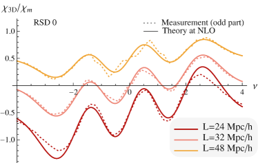
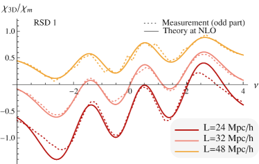
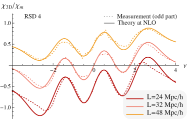
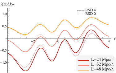
Figure 7: Top left panel: first non-Gaussian correction of the 3D Euler characteristic  as a function of smoothing (as labeled) measured (dotted lines) and predicted (plain line) in horizon $4\pi$ simulation in real space. Each curve has been normalized by the maximum of the Gaussian component of the Euler characteristic. Those corresponding to different smoothing length have been shifted for clarity. Top right panel: same as top left panels, but in redshift space. Bottom left panel: same as top right panels, but redshift displacements were boosted by a factor of four. Bottom right panel: theoretical prediction in real space and boosted redshift space. For these ranges of smoothing the theory predicts well the Euler characteristic  to first order in non-Gaussianity, in particular for low-intermediate thresholds. The difference in the Euler characteristic  introduced by redshift distortion (even boosted by a factor of four) is rather small.

illustrates this for the 3D Euler characteristic. First, note that the theory mimics very well the measurement. This figure also shows that the difference between real and redshift space is indeed small for the first correction from Gaussianity. But in 2D, this difference increases as seen in Figure 8

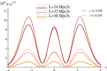
Figure 8: Prediction for the 2D Euler characteristic  in redshift space along (dashed lines) and perpendicular (solid lines) to the LOS with cumulants measured in the horizon $4\pi$ simulation. There is a clear dependence on the angle between the slice and the LOS, especially for smaller smoothing.

which shows how the correction from Gaussianity depends on the angle between the LOS and the slice on which the 2D Euler characteristic  is computed.

5.4.2 Minkowski functionals for halo catalogues

The Friend-of-Friend Algorithm (hereafter FOF, Huchra & Geller, 1982) was used over $18^{3}$ overlapping subsets of the simulation with a linking length of 0.2 times the mean inter-particular distance to define dark matter halos. In the present work, we only consider halos with more than 40 particles, which corresponds to a minimum halo mass of $3\cdot 10^{11}M_{\odot}$ (the particle mass is $7.7\cdot 10^{9}M_{\odot}$). The mass dynamical range of this simulation spans about 5 decades. Overall, the catalog contains 43 million dark halos. The density of dark halos in real space and redshift space was re-sampled over a $512^{3}$ grid with box size $2000\leavevmode\nobreak\ \mathrm{Mpc}/h$ (in redshift space, after shifting the z-ordinate of the halo by its velocity along that direction divided by the Hubble constant, $H_{0}$) and smoothed with a Gaussian filter of width $\sigma=$ 16, 24… up to $94$ Mpc$/h$.

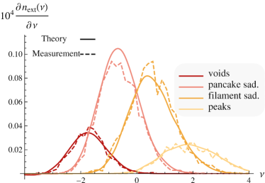
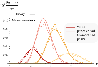
Figure 9: Left panel: The distribution of 3D extrema in real space as a function of threshold $\nu$ in real space, as predicted (solid) and measured (dashed) in dark matter halo catalogue of the horizon $4\pi$ simulation smoothed over 48 Mpc/h. Right panel: same as left panel but in redshift space.

For each cube in real and redshift space the number density of extrema is computed by a local quadratic fit to the function profile with control over the double counting of the neighbouring extrema (see Pogosyan et al. (2011) for the technique description and Colombi et al. (2000) for a first application). The relevant 35 cumulants are computed via fast Fourier transform. Figure 9 displays the corresponding predicted (solid line) and measured (dashed line) number count difference in real space (left panel) and redshift space (right panel). Note that redshift and real space extrema counts are almost indistinguishable. Indeed, for this biased population, $b_{1}$ is large ($\sim$2) and $f/b_{1}$ is small enough.

5.5 A cosmic fiducial experiment: measuring $\beta$ and $\sigma$ via slicing along and perpendicular to the line of sight

As mentioned in Section 4, the angle-dependence of the 2D Minkowski functionals allows us to probe $\beta$. Indeed, equations (43)-(54)-(60) displays a functional dependence on $\theta_{\cal S/L}$. At Gaussian order first, it appears that

$$\chi_{2\textrm{D}}^{(0)}(\nu,\theta_{\cal S})\propto\sqrt{1-\beta_{\sigma}\sin^{2}\theta_{\cal S}}\,,$$ (99)

so that measuring the Gaussian part of the 2D Euler characteristic  in different slices (with different orientation relative to the LOS) can give access to $\beta_{\sigma}=1-\sigma_{1\perp}^{2}/2\sigma_{1\parallel}^{2}=\frac{4}{5}\beta+{\cal O}(\beta^{2})$. For example, in the most favorable case of $\theta_{1}=\pi/2$ and $\theta_{2}=0$, one have directly access to

$$\frac{\chi_{2\textrm{D}}^{(0)}(\nu,\theta_{1})}{\chi_{2\textrm{D}}^{(0)}(\nu,\theta_{2})}=\sqrt{\frac{1-\beta_{\sigma}\sin^{2}\theta_{1}}{1-\beta_{\sigma}\sin^{2}\theta_{2}}}=\sqrt{1-\beta_{\sigma}}=1-\frac{2}{5}\beta+{\cal O}(\beta^{2})\,.$$ (100)

Contour crossing statistics have the same angle-dependence as 2D Euler characteristic  at Gaussian order. The ${\cal N}_{2}$ statistics (area of isocontours) leads in turn

$$\frac{{\cal N}_{2}^{(0)}(\nu,\theta_{1})}{{\cal N}_{2}^{(0)}(\nu,\theta_{2})}=\frac{E(\tilde{\beta}_{\sigma}(\theta_{1}))\sqrt{1-\tilde{\beta}_{\sigma}(\theta_{2})}}{E(\tilde{\beta}_{\sigma}(\theta_{2}))\sqrt{1-\tilde{\beta}_{\sigma}(\theta_{1})}}=\frac{\pi}{2}\frac{\sqrt{1-\beta_{\sigma}}}{E(\beta_{\sigma})}=1-\frac{1}{5}\beta+{\cal O}(\beta^{2})\,.$$ (101)

Note that beyond a simple overall amplitude effect (which is enough to measure $\beta$ alone), this angle-dependence also arises in the first non-Gaussian correction as plotted in Figure 5.

If the value of $\beta$ is important on its own (e.g to study the bias or to test modifications of gravity), it is also of prime importance to measure $D(z)$ as it allows us to map the dispersion in redshift space, $\sigma$, into its value in real space, $\sigma_{0}\propto D(z)$. One way to proceed is to use the Gaussian term to put constraints on $\beta$ and then the non-Gaussian correction for $\sigma$ (the amplitude of which is not probed by the Gaussian part). Indeed, following Gay et al. (2012), the theory presented in Section 4 should allow us to measure the dispersion of the field in redshift space $\sigma$ from the amplitude of the departure from non-Gaussianity. As equation (101) demonstrates, the comparison of the 2D Minkowski functionals in planes parallel and perpendicular to the LOS allows us to measure independently $\beta=f/b$. Hence Minkowski functionals in redshift space yield a geometric estimate of the real-space field dispersion, $\sigma_{0}$, via

$$\sigma_{0}=\sigma/\sqrt{1+{2}\beta/3+{\beta^{2}}/{5}}.$$ (102)

Let us apply this scheme to measure $\beta$ and $\sigma_{0}$ in a fiducial experiment. Minkowski functionals are measured from our set of 19 scale-invariant (n=-1) $256^{3}$ dark matter simulations smoothed over 15 pixels, corresponding to $\sigma_{0}=0.18$ and displayed in Figure 4. A first step is to use the Gaussian term of the 1D and 2D statistics, while varying the angle of the slices to constrain $\beta$ using equations (100)-(101). For that purpose, we extract the even part of ${\cal N}_{2}$ (to get rid of odd parity effects arising from the first NLO correction) and restrict ourselves to the intermediate domain $-1.2<\nu<1.2$ where the Gaussian term is dominant. The resulting constraints on $\beta$ are found to be $\hat{\beta}=1.04\pm 0.05\,,$ and illustrated on Figure 10 (left panel). The same analysis on the other 1D (${\cal N}_{1}$) and 2D statistics (2D genus) leads to similar constraints. The next step is to fit the first non-Gaussian correction of each statistics with PT predictions in order to constrain $\sigma$. The predictions at first order are expressed as a function of the contrast $\nu$ and $\sigma$ only using Table 4. The value of the free parameter $\sigma$ in the model is then constrained by fitting the odd part of the data (which is dominated by the first non-Gaussian correction for intermediate contrasts). The result for ${\cal N}_{2}$ is shown in Figure 10 (right panel) and yields $\hat{\sigma}=0.22\pm 0.08$. The other statistics give similar results e.g for the 3D Euler characteristic  $\hat{\sigma}=0.26\pm 0.06.$ Altogether, using $\sigma$ as measured by a 3D probe, $\chi_{\textrm{3D}}$, and $\beta$ by a 2D statistics, ${\cal N}_{2}$, we finally get $\hat{\sigma}_{0}=0.18\pm 0.04$, which is fully consistent with the underlying dispersion in our mocks. The accuracy on the measurement of $\beta$ and $D(z)$ through $\sigma_{0}$ can naively be scaled to the expected accuracy for a Euclid-like survey (assuming one quarter of the sky is observed) leading to a relative 0.3% precision on $\beta$ and 1.5% on $D(z)$ at redshift zero. See also Gay et al. (2012), which translates this accuracy in terms of estimates for the dark energy parameters $w_{0},w_{a}$.

It is worth noting that in this simple fiducial experiment, several assumptions were made : first, we assumed we knew the contrast, $\nu$, while in realistic surveys, the accessible quantity is $\nu_{f}$ (see section 4.5.1); for the simulation, the cosmology is not $\Lambda$CDM but Einstein-de Sitter with a scale-invariant initial power spectrum; finally the error on the estimated $\sigma$ depends on the accuracy of the theory used to predict the cumulants (Standard Perturbation Theory here which is known to perform somewhat poorly in redshift space). No account of masking, redshift evolution of S/N ratio or finite survey volume, nor comparison with other dark energy probes was attempted. Carrying out the road map sketched in this section while addressing these issues should be one of the target of the upcoming surveys that have been planned specifically to probe dark energy, either from ground-based facilities (eg BigBOSS, VST-KIDS, DES, Pan-STARRS, LSST) or space-based observatories (EUCLID(Laureijs et al., 2011), SNAP and JDEM).

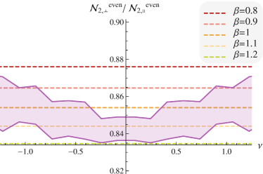
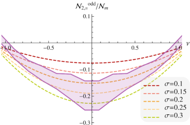
Figure 10: Reconstructed $\beta$ from the Gaussian part of ${\cal N}_{2}$ (left panel) and $\sigma$ from its non-Gaussian correction (right panel) .

6 Conclusion

This paper has placed on a firm footing the statistical analysis of topological sets in anisotropic spaces. Specifically, it has presented extensions of Matsubara (1996) and Gay et al. (2012) in two directions: it has accounted for anisotropic fields and non-Gaussianity for all Minkowski’s functionals. The main results of this work are: i) the anisotropic JPDF in 2 and 3D: a new building block for redshift space analysis; ii) the analytical Euler characteristic at all order in 2D/3D (and therefore the rare event limit for extrema counts); iii) other Minkowski functionals and extrema counts to first order in non-Gaussian correction in anisotropic space; iv) and extension of PT for the relevant cumulants. The theory presented in Sections 3 and 4 makes no assumption about the origin of the anisotropy and could therefore be implemented in contexts beyond astrophysics.

In the context of cosmology, the theoretical expectations were robustly derived both in invariant and field variables, and checked against Monte Carlo simulations of $f_{\mathrm{{nl}}}$ models, scale-invariant dark matter simulations, and $\Lambda$CDM simulations (both for DM and halo catalogues). It was shown how to use these predictions to measure $\sigma_{\mathrm{0}}$ and $\beta$ as a function of redshift. The implication of the invariance of Minkowski functionals and extrema counts versus monotonic mapping on the relevant combinations of cumulants (i.e. projections of the bispectrum) was made explicit. Its relevance for modified gravity probes was discussed. The implementation on dark matter halos of $\Lambda$CDM simulations for biased populations with $M>10^{11}M_{\odot}$, allowed us to quantify and formalize the (weak) effect of redshift distortion on the 3D geometric descriptors of the field. This weak sensitivity reflects the robustness of topological estimates. In contrast, the comparison of 2D slices perpendicular and parallel to the LOS should allow us to also measure $\sigma(z)$ and correct it for $\Omega_{m}^{\gamma}/b_{1}$ as demonstrated in a fiducial experiment. At scales above $\sim$50 Mpc$/h$ it has been found that standard perturbation theory allows us to predict the theoretical cumulants at the level of accuracy required to match the measured cumulants from simulations within a range of contrast $\nu\in[-2,2]$. As Minkowski functionnals are configuration space probes, we can expect a better convergence of (extended) PT for these contrasts which are less sensitive to the dynamics of very non-linear regions.

Improvements beyond the scope of this paper include i) improving perturbation theory in redshift space (while implementing variations of the streaming model (see Scoccimarro, 2004; Taruya et al., 2010, for instance) and/or anisotropic smoothing; ii) departing from the plane parallel approximation while constructing a full-sky prescription for non-Gaussian Minkowski functionals of realistic catalogues; iii) extending the prediction to the statistics of the skeleton and walls; iv) propagating to cosmic parameter estimation the residual mis-fits; v) extending the prediction of the JPDF to N-point statistics for non-local analysis (e.g. void size and non-linear N-points peak statistics); vi) exploring alternative expansion to the Gram-Charlier’s vii) deriving the statistics of errors on one-point statistics such as those presented in this paper; viii) implementing the relevant theory on realistic mocks and demonstrating pros and cons of geometrical probes (e.g. in the presence of masks), and contrast those to existing dark energy probes (lensing, SN1a, etc..).

In the context of upcoming 3D spectroscopic surveys such as Euclid, the statistical analysis of the geometry of our redshift-distorted Universe will allow us to robustly measure weighted moments of the multi-spectra as a function of redshift, and henceforth quantify the cosmic evolution of the equation of state of dark energy and possible departure from GR.

Appendix A Spectral parameters and cumulants

A.1 Relations with the parametrization of Matsubara (1996)

At linear order, the redshift distortion, equation (83) reduces to Kaiser (1987) result in equation (12). Matsubara (1996) defines the dispersions and angular moments

$$\sigma_{j}^{2}(R)\equiv\frac{1}{2\pi^{2}}\int\mathrm{d}k\;k^{2+2j}P^{(r)}(k)\,W^{2}(kR)\,,\quad C_{j}(f/b)=\frac{1}{2}\int_{-1}^{1}\mathrm{d}\mu\;\mu^{2j}(1+fb^{-1}\mu^{2})^{2}\,,$$ (103)

and uses the normalized quantities

$$\alpha\equiv\frac{\delta_{R}^{(s)}}{{\sigma_{0}\sqrt{C_{0}}}},\quad\beta_{i}\equiv\frac{\partial_{i}\delta_{R}^{(s)}}{{\sigma_{0}\sqrt{C_{0}}}}\quad\textrm{and}\quad\omega_{ij}\equiv\frac{\partial_{i}\partial_{j}\delta_{R}^{(s)}}{{\sigma_{0}\sqrt{C_{0}}}},$$ (104)

to describe the smoothed density contrast in redshift space $\delta_{R}^{(s)}$ and its derivatives. Our variables relate to these as

$$x=\alpha,\quad x_{I}=\frac{\sqrt{C_{0}}\sigma_{0}}{\sigma_{1\perp}}\beta_{I},\quad x_{3}=\frac{\sqrt{C_{0}}\sigma_{0}}{\sigma_{1\parallel}}\beta_{3},\quad x_{IJ}=\frac{\sqrt{C_{0}}\sigma_{0}}{\sigma_{2\perp}}\omega_{IJ}\textrm{ and }x_{33}=\frac{\sqrt{C_{0}}\sigma_{0}}{\sigma_{2\parallel}}\omega_{33},$$ (105)

where $I,J\in\{1,2\}$, so that

$$\sigma^{2}=C_{0}\sigma_{0}^{2},\quad\sigma_{1\perp}^{2}=(C_{0}-C_{1})\sigma_{1}^{2},\quad\sigma_{1\parallel}^{2}=C_{1}\sigma_{1}^{2},\quad\sigma_{2\perp}^{2}=(C_{0}-2C_{1}+C_{2})\sigma_{2}^{2},\quad\sigma_{2\parallel}^{2}=C_{2}\sigma_{2}^{2},$$ (106)

with

$$C_{0}=1+\frac{2f}{3b}+\frac{f^{2}}{5b^{2}},\quad C_{1}=\frac{1}{3}+\frac{2f}{5b}+\frac{f^{2}}{7b^{2}},\quad C_{2}=\frac{1}{5}+\frac{2f}{7b}+\frac{f^{2}}{9b^{2}}\,.$$ (107)

In terms of these variables, both formulations are in exact agreement. In the isotropic Gaussian limit (i.e the linear regime with no redshift correction) $C_{0}=1$, $C_{1}=1/3$, $C_{2}=1/5$.

A.2 Inter-relations between the moments of random fields and simplification of Gay et al. (2012) results

Not all cumulants of the field and its derivatives that appear in Gram-Charlier expansion are independent. Relations between the cumulants can be established, for instance, by expressing statistical averages as averages over spatial coordinates using homogeneity of the statistics and utilizing integration by parts. The details of the results depend on the properties of the manifold, in this paper we limit ourselves to the theory in the flat infinite Euclidean space. As an example

$$\langle x^{2}x_{33}\rangle=\lim_{V\to\infty}\frac{1}{V}\int_{V}dVx^{2}x_{33}=-\gamma_{\parallel}\lim_{V\to\infty}\frac{2}{V}\int_{V}dVxx_{3}^{2}=-2\gamma_{\parallel}\langle xx_{3}^{2}\rangle\,,$$ (108)

where the boundary term vanishes as volume $V$ is taken in the infinite limit. A similar procedure shows that, e.g., $\langle x_{1}^{2}x_{11}\rangle=0$.

Proceeding in this manner one can establish for isotropic fields several useful general relations that involve the rotation invariants $I_{s}$ of the Hessian matrix $x_{ij}$ :

$$\langle x^{n}I_{1}\rangle = -n\gamma\langle x^{n-1}q^{2}\rangle,$$ (109)

$$\langle x^{n}I_{2}\rangle = -\frac{3}{4}n\gamma\langle x^{n-1}q^{2}I_{1}\rangle-\frac{1}{4}n(n-1)\gamma^{2}\langle x^{n-2}q^{4}\rangle,$$ (110)

$$\langle x^{n}I_{s}\rangle = -\frac{1}{s}\sum_{k=1}^{\mathrm{min}(s,n)}\frac{s+k}{(2k)!!}\frac{n!}{(n-k)!}\gamma^{k}\left\langle x^{n-k}q^{2k}I_{s-k}\right\rangle\,,s\geq 1\,,I_{0}=1.$$ (111)

These relations are valid in any dimensions, for correspondingly defined $I_{s}$’s, and also hold for the cumulants as well as the moments.

A.2.1 Isotropic 3D Euler characteristic

The relations (109-111) allow to simplify the expression for the Euler characteristic given by Gay et al. (2012) for isotropic fields. Indeed, these authors found

$$\chi^{\textrm{iso}(0)}_{3\textrm{D}}(\nu)=\frac{e^{-\nu^{2}/2}}{(2\pi)^{2}R_{\star}^{3}}\frac{\sqrt{3}}{9}\gamma^{3}H_{2}(\nu)\,,$$ (112)

$$\chi^{\textrm{iso}(1)}_{3\textrm{D}}(\nu)=\frac{e^{-\nu^{2}/2}}{(2\pi)^{2}R_{\star}^{3}}\frac{\sqrt{3}}{9}\left[\frac{1}{6}\gamma^{3}\left\langle x^{3}\right\rangle H_{5}(\nu)-\frac{3}{2}\left(\gamma^{3}\left\langle xq^{2}\right\rangle+\gamma^{2}\left\langle x^{2}J_{1}\right\rangle\right)H_{3}(\nu)+9\left(\frac{1}{2}\gamma^{2}\left\langle q^{2}J_{1}\right\rangle+\gamma\left\langle xI_{2}\right\rangle\right)H_{1}(\nu)\right]\,,$$ (113)

$$\chi^{\textrm{iso}(2)}_{3\textrm{D}}(\nu)=\frac{e^{-\nu^{2}/2}}{(2\pi)^{2}R_{\star}^{3}}\frac{\sqrt{3}}{9}\left[-\left(\frac{27}{2}\gamma\langle q^{2}I_{2}\rangle_{\mathrm{c}}+27\langle xI_{3}\rangle_{\mathrm{c}}\right)H_{0}(\nu)+\left(\frac{9}{8}\gamma^{3}\langle q^{4}\rangle_{c}+\frac{9}{2}\gamma^{2}\langle xq^{2}J_{1}\rangle_{\mathrm{c}}+\frac{9}{2}\gamma\langle x^{2}I_{2}\rangle_{\mathrm{c}}\right)H_{2}(\nu)\right.$$

$$-\left(\frac{3}{4}\gamma^{3}\langle x^{2}q^{2}\rangle_{\mathrm{c}}+\frac{1}{2}\gamma^{2}\langle x^{3}J_{1}\rangle_{\mathrm{c}}\right)H_{4}(\nu)+\frac{1}{24}\gamma^{3}\langle x^{4}\rangle_{\mathrm{c}}H_{6}(\nu)+\left(\frac{135}{16}\gamma\langle q^{2}J_{1}\rangle^{2}+\frac{27}{2}\langle q^{2}J_{1}\rangle\langle xI_{2}\rangle+\frac{81}{2}\langle xq^{2}\rangle\langle I_{3}\rangle\right)H_{0}(\nu)$$

$$-\left(\frac{45}{4}\gamma^{2}\langle xq^{2}\rangle\langle q^{2}J_{1}\rangle+\frac{9}{2}\gamma\langle q^{2}J_{1}\rangle\langle x^{2}J_{1}\rangle+\frac{27}{2}\gamma\langle xq^{2}\rangle\langle xI_{2}\rangle+\frac{9}{2}\langle x^{2}J_{1}\rangle\langle xI_{2}\rangle+\frac{9}{2}\langle x^{3}{\rangle\langle}I_{3}\rangle\right)H_{2}(\nu)$$

$$+\left(\frac{15}{8}\gamma^{3}\langle xq^{2}\rangle^{2}+\frac{3}{4}\gamma^{2}\langle x^{3}\rangle\langle q^{2}J_{1}\rangle+\frac{9}{4}\gamma^{2}\langle xq^{2}\rangle\langle x^{2}J_{1}\rangle+\frac{3}{4}\gamma\langle x^{2}J_{1}\rangle^{2}+\frac{3}{2}\gamma\langle x^{3}\rangle\langle xI_{2}\rangle\right)H_{4}(\nu)$$

$$\left.-\left(\frac{1}{4}\gamma^{3}\langle xq^{2}\rangle\langle x^{3}\rangle+\frac{1}{4}\gamma^{2}\langle x^{3}\rangle\langle x^{2}J_{1}\rangle\right)H_{6}(\nu)+\frac{1}{72}\gamma^{3}\langle x^{3}\rangle^{2}H_{8}(\nu)\right],$$ (114)

where $R_{\star}=\sigma_{1}/\sigma_{2}$. Using equations (109)-(111), the equations (112)-(113) can be rewritten up to NLO as

$$\chi^{\textrm{iso}(0+1)}_{3\textrm{D}}(\nu)=\frac{e^{-\nu^{2}/2}}{(2\pi)^{2}}\frac{\sigma_{1}^{3}}{\sigma^{3}}\frac{\sqrt{3}}{9}\left[H_{2}(\nu)+\frac{1}{6}H_{5}(\nu)\left\langle x^{3}\right\rangle+\frac{3}{2}H_{3}(\nu)\left\langle xq^{2}\right\rangle-\frac{9}{4}H_{1}(\nu)\frac{1}{\gamma}\left\langle q^{2}J_{1}\right\rangle\right]\,,$$ (115)

which is the form we quote in equation (38). The NNLO, ${{\cal O}(\sigma^{2})}$, term can be also simplified from equation (114) to a more compact form

$$\chi_{3\textrm{D}}^{\textrm{iso}(2)}(\nu)=\frac{e^{-\nu^{2}/2}}{(2\pi)^{2}}\frac{\sigma_{1}^{3}}{\sigma^{3}}\frac{\sqrt{3}}{9}\times\\ \left[H_{0}(\nu)\left(\frac{9}{2}\gamma^{-2}\left\langle q^{2}I_{2}\right\rangle_{c}-\frac{27}{16}\gamma^{-2}\left\langle J_{1}q^{2}\right\rangle^{2}\right)+H_{2}(\nu)\left(-\frac{9}{8}\left\langle q^{4}\right\rangle_{c}-\frac{9}{4}\gamma^{-1}\left\langle xq^{2}J_{1}\right\rangle_{c}+\frac{9}{8}\gamma^{-1}\left\langle xq^{2}\right\rangle\left\langle J_{1}q^{2}\right\rangle\right)\right.\\ \left.+H_{4}(\nu)\left(\frac{3}{4}\left\langle x^{2}q^{2}\right\rangle_{c}+\frac{3}{8}\left\langle xq^{2}\right\rangle^{2}-\frac{3}{8}\gamma^{-1}\left\langle x^{3}\right\rangle\left\langle J_{1}q^{2}\right\rangle\right)+H_{6}(\nu)\left(\frac{1}{24}\left\langle x^{4}\right\rangle_{c}+\frac{1}{4}\left\langle x^{3}\right\rangle\left\langle xq^{2}\right\rangle\right)+H_{8}(\nu)\frac{1}{72}\left\langle x^{3}\right\rangle^{2}\right]\,.$$ (116)

A.2.2 Isotropic 2D Euler characteristic

The same procedure holds for the 2D Euler characteristic for which the expression given by Gay et al. (2012) in terms of a 2D isotropic field $x$

$$\chi_{2\textrm{D}}^{\textrm{iso}(0)}(\nu)=\frac{e^{-\nu^{2}/2}}{(2\pi)^{3/2}}\frac{1}{2R_{\star}^{2}}\gamma^{2}H_{1}(\nu),$$ (117)

$$\chi_{2\textrm{D}}^{\textrm{iso}(1)}(\nu)=\frac{e^{-\nu^{2}/2}}{(2\pi)^{3/2}}\frac{1}{2R_{\star}^{2}}\left[\frac{1}{3!}\gamma^{2}\left\langle x^{3}\right\rangle H_{4}\left(\nu\right)-\left(\gamma^{2}\left\langle xq^{2}\right\rangle+{\gamma}\left\langle x^{2}J_{1}\right\rangle\right)H_{2}(\nu)+\left({2}{\gamma}\left\langle q^{2}J_{1}\right\rangle+4\left\langle xI_{2}\right\rangle\right)\right],$$ (118)

$$\chi_{2\textrm{D}}^{\textrm{iso}(2)}(\nu)=\frac{e^{-\nu^{2}/2}}{(2\pi)^{3/2}}\frac{1}{2R_{\star}^{2}}\left[\left(\frac{\gamma^{2}}{2}\langle q^{4}\rangle_{\mathrm{c}}+2\gamma\langle xq^{2}J_{1}\rangle_{\mathrm{c}}+2\langle x^{2}I_{2}\rangle_{\mathrm{c}}\right)H_{1}(\nu)-\left(\frac{1}{2}\gamma^{2}\langle x^{2}q^{2}\rangle_{\mathrm{c}}+\frac{\gamma}{3}\langle x^{3}J_{1}\rangle_{\mathrm{c}}\right)H_{3}(\nu)+\frac{\gamma^{2}}{24}\langle x^{4}\rangle_{\mathrm{c}}H_{5}(\nu)\right.$$

$$-\left(4\gamma\langle xq^{2}\rangle\langle q^{2}J_{1}\rangle+\langle q^{2}J_{1}\rangle\langle x^{2}J_{1}\rangle+4\langle xq^{2}\rangle\langle xI_{2}\rangle\right)H_{1}(\nu)-\left(\frac{{\gamma^{2}}}{6}\langle xq^{2}\rangle\langle x^{3}\rangle+\frac{\gamma}{6}\langle x^{3}\rangle\langle x^{2}J_{1}\rangle\right)H_{5}(\nu)+\frac{\gamma^{2}}{72}\langle x^{3}\rangle^{2}H_{7}(\nu)\,$$

$$\left.+\left(\gamma^{2}\langle xq^{2}\rangle^{2}+\frac{\gamma}{3}\langle x^{3}\rangle\langle q^{2}J_{1}\rangle+\gamma\langle xq^{2}\rangle\langle x^{2}J_{1}\rangle+\frac{1}{4}\langle x^{2}J_{1}\rangle^{2}+\frac{2}{3}\langle x^{3}\rangle\langle xI_{2}\rangle\right)H_{3}(\nu)\right]$$ (119)

can be simplified up to NLO to

$$\chi_{2\textrm{D}}^{\textrm{iso}(0+1)}(\nu)=\frac{\sigma_{1}^{2}}{2\sigma^{2}}\frac{e^{-\nu^{2}/2}}{(2\pi)^{3/2}}\left[H_{1}(\nu)+\frac{1}{3!}H_{4}\left(\nu\right)\left\langle x^{3}\right\rangle+H_{2}(\nu)\left\langle xq^{2}\right\rangle-\gamma^{-1}\left\langle q^{2}J_{1}\right\rangle+{\cal O}(\sigma^{2})\right],$$ (120)

which is to be compared with expression (44) for the Euler characteristic on 2D slices. The NNLO term adds:

$$\chi_{2\textrm{D}}^{\textrm{iso}(2)}(\nu)=\frac{\sigma_{1}^{2}}{2\sigma^{2}}\frac{e^{-\nu^{2}/2}}{(2\pi)^{3/2}}\left[H_{1}(\nu)\left(-\frac{1}{2}\left\langle q^{4}\right\rangle_{c}-\gamma^{-1}\left\langle xq^{2}J_{1}\right\rangle_{c}+\gamma^{-1}\left\langle xq^{2}\right\rangle\left\langle q^{2}J_{1}\right\rangle\right)\right.\\ \left.+H_{3}(\nu)\left(\frac{1}{2}\left\langle x^{2}q^{2}\right\rangle_{c}-\frac{1}{6}{\gamma^{-1}}\left\langle x^{3}\right\rangle\left\langle q^{2}J_{1}\right\rangle\right)+H_{5}(\nu)\left(\frac{1}{24}\left\langle x^{4}\right\rangle_{c}+\frac{1}{6}\left\langle xq^{2}\right\rangle\left\langle x^{3}\right\rangle\right)+H_{7}(\nu)\frac{1}{72}\left\langle x^{3}\right\rangle^{2}\right].$$ (121)

Appendix B ($f_{\mathrm{{nl}}}$,$g_{\mathrm{{nl}}}$) non-Gaussian field toy models

B.1 $f_{\mathrm{{nl}}}$ toy model for the field

Let us briefly describe the toy model used in the main text to validate our predictions for extrema counts and Minkowski functionals in 2D and 3D. If X is a Gaussian (possibly anisotropic) field with zero mean and variance $\left\langle X^{2}\right\rangle=\sigma_{0}^{2}$, let us define the following non-Gaussian field

$$X^{\mathrm{NG}}=X+\frac{f_{\mathrm{{nl}}}}{\sigma_{0}}\left(X^{2}-\sigma_{0}^{2}\right)+\frac{g_{\mathrm{{nl}}}}{\sigma_{0}^{2}}\left(X^{3}-3\sigma_{0}^{2}X\right)\,.$$ (122)

For the purpose of this paper, let us define $X$ as a Kaiser transform of a Gaussian isotropic field, $X^{\mathrm{G}}$, which can be written in Fourier space, following equation (11), as

$$\hat{X}_{k}=(1+f\mu^{2})\hat{X}^{\mathrm{G}}_{k},\quad\mathrm{with}\quad\mu=k_{\parallel}/k.$$ (123)

Then any Minkowski functional or extrema count of this non-Gaussian field can simply be written in terms only of $f$, $f_{\mathrm{{nl}}}$, $g_{\mathrm{{nl}}}$ and $\sigma$’s (or $n$ for a scale invariant powerspectrum). Indeed, one can easily show that the spectral parameters of the non-Gaussian field are the following in terms of the spectral parameters of $X$ (in 2D): $\tilde{\sigma}^{2}=(1+2f_{\mathrm{{nl}}}^{2})\sigma_{0}^{2}$, $\tilde{\sigma}_{1\perp}^{2}=(1+4f_{\mathrm{{nl}}}^{2})\sigma_{1\perp}^{2}$, $\tilde{\sigma}_{1\parallel}^{2}=(1+4f_{\mathrm{{nl}}}^{2})\sigma_{1\parallel}^{2}$, $\tilde{\sigma}_{2\perp}^{2}=(1+4f_{\mathrm{{nl}}}^{2}+{12}f_{\mathrm{{nl}}}^{2}\gamma_{\perp}^{2})\sigma_{2\perp}^{2}$, $\tilde{\sigma}_{2\parallel}^{2}=(1+4f_{\mathrm{{nl}}}^{2}+12f_{\mathrm{{nl}}}^{2}\gamma_{\parallel}^{2})\sigma_{2\parallel}^{2}$ and $\tilde{\sigma}_{Q}^{2}=(1+4f_{\mathrm{{nl}}}^{2}+4f_{\mathrm{{nl}}}^{2}\gamma_{\perp}\gamma_{\parallel}/\gamma_{2})\sigma_{Q}^{2}$ where in turn the spectral parameters of $X$ can be expressed as functions of the spectral parameters of $X^{\mathrm{G}}$ : $\sigma_{0}^{2}=(1+f+3f^{2}/8)\sigma^{2}$, $\sigma_{1\parallel}^{2}=1/16(8+12f+5f^{2})\sigma_{1}^{2}$, $\sigma_{1\perp}^{2}=1/16(8+4f+f^{2})\sigma_{1}^{2}$, $\sigma_{2\parallel}^{2}=1/128(48+80f+35f^{2})\sigma_{2}^{2}$, $\sigma_{2\perp}^{2}=1/128(48+16f+3f^{2})\sigma_{2}^{2}$ and $\sigma_{Q}^{2}=1/128(16+16f+5f^{2})\sigma_{2}^{2}$. In 2D, the three-point cumulants of the non-Gaussian field can also be computed: $\left\langle x^{3}\right\rangle=f_{\mathrm{{nl}}}(6+8f_{\mathrm{{nl}}}^{2})/(1+2f_{\mathrm{{nl}}}^{2})^{3/2}$, $\left\langle xq_{||,\perp}^{2}\right\rangle=4f_{\mathrm{{nl}}}\sqrt{1+2f_{\mathrm{{nl}}}^{2}}/(1+4f_{\mathrm{{nl}}}^{2})$ and $\left\langle J_{1\perp}q_{||}^{2}\right\rangle/\gamma_{\perp}=-4f_{\mathrm{{nl}}}\sqrt{1+2f_{\mathrm{{nl}}}^{2}}/(1+4f_{\mathrm{{nl}}}^{2})$.

In 3D, similar relations hold: $\tilde{\sigma}^{2}=(1+2f_{\mathrm{{nl}}}^{2})\sigma_{0}^{2}$, $\tilde{\sigma}_{1\perp}^{2}=(1+4f_{\mathrm{{nl}}}^{2})\sigma_{1\perp}^{2}$, $\tilde{\sigma}_{1\parallel}^{2}=(1+4f_{\mathrm{{nl}}}^{2})\sigma_{1\parallel}^{2}$, $\tilde{\sigma}_{2\perp}^{2}=(1+4f_{\mathrm{{nl}}}^{2}+{8}f_{\mathrm{{nl}}}^{2}\gamma_{\perp}^{2})\sigma_{2\perp}^{2}$, $\tilde{\sigma}_{2\parallel}^{2}=(1+4f_{\mathrm{{nl}}}^{2}+12f_{\mathrm{{nl}}}^{2}\gamma_{\parallel}^{2})\sigma_{2\parallel}^{2}$ and $\tilde{\sigma}_{Q}^{2}=(1+4f_{\mathrm{{nl}}}^{2}+4f_{\mathrm{{nl}}}^{2}\gamma_{\perp}\gamma_{\parallel}/\gamma_{2})\sigma_{Q}^{2}$ where again it can be related to the spectral parameters of the isotropic Gaussian field $X$ : $\sigma_{0}^{2}=(1+2f/3+f^{2}/5)\sigma^{2}$, $\sigma_{1\parallel}^{2}=(1/3+2f/5+f^{2}/7)\sigma_{1}^{2}$, $\sigma_{1\perp}^{2}=(2/3+4f/15+2f^{2}/35))\sigma_{1}^{2}$, $\sigma_{2\parallel}^{2}=(1/5+2f/7+f^{2}/9)\sigma_{2}^{2}$, $\sigma_{2\perp}^{2}=(8/15+16f/105+8f^{2}/315)\sigma_{2}^{2}$ and $\sigma_{Q}^{2}=(2/15+4f/35+2f^{2}/63)\sigma_{2}^{2}$; the three-point cumulants of interest being: $\left\langle x^{3}\right\rangle=f_{\mathrm{{nl}}}(6+8f_{\mathrm{{nl}}}^{2})/(1+2f_{\mathrm{{nl}}}^{2})^{3/2}$, $\left\langle xq_{||,\perp}^{2}\right\rangle=4f_{\mathrm{{nl}}}\sqrt{1+2f_{\mathrm{{nl}}}^{2}}/(1+4f_{\mathrm{{nl}}}^{2})$, $\left\langle J_{1\perp}q_{\perp}^{2}\right\rangle/\gamma_{\perp}=-2f_{\mathrm{{nl}}}\sqrt{1+2f_{\mathrm{{nl}}}^{2}}/(1+4f_{\mathrm{{nl}}}^{2})$ and $\left\langle J_{1\perp}q_{||}^{2}\right\rangle/\gamma_{\perp}=-4f_{\mathrm{{nl}}}\sqrt{1+2f_{\mathrm{{nl}}}^{2}}/(1+4f_{\mathrm{{nl}}}^{2})$.

Figures 11 and 12 illustrate the interplay between anisotropy and non-Gaussianity that this paper investigates on this example of the “$f_{nl}$” toy model. It presents the 2D/3D Euler characteristic of a mildly non-Gaussian anisotropic field for different values of the quadratic parameter $f_{\mathrm{{nl}}}$ and anisotropy, $f$. Both predictions derived in Sections (4.2.1) and (4.2.2), and measurements from Monte Carlo realizations of the corresponding field are shown. The agreement between theory and measurements is very good. As expected, in 2D the effect of anisotropy is larger than in 3D.

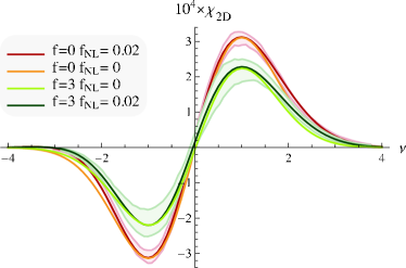
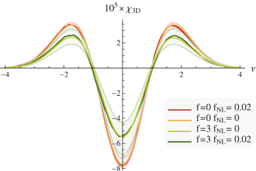
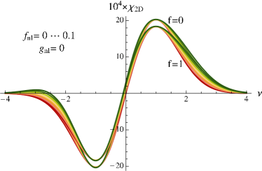
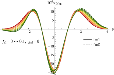
Figure 11: 2D (left) and 3D (right) Euler characteristic of a mildly non-Gaussian anisotropic field in a toy model. Top left: Comparison with measurements for different values of quadratic parameter $f_{\mathrm{{nl}}}$ and anisotropy, $f$ as labeled. The shaded area corresponds to the one sigma measurements error on realisations of the non-Gaussian fields. The overall amplitude has been rescaled by $10^{4}$. Note both the change in amplitude with $f$ and the distortion in the tails of the distribution with $f_{\mathrm{{nl}}}$ which are well fitted by the model. Bottom left panel: theoretical evolution of the 2D Euler characteristic as a function of $f_{\mathrm{{nl}}}$ as labeled for $f=0$ and $f=1$. For this level of anisotropy, the difference in amplitude is less significant. Top right and bottom right panels: same as the correspondent left panels in 3D.

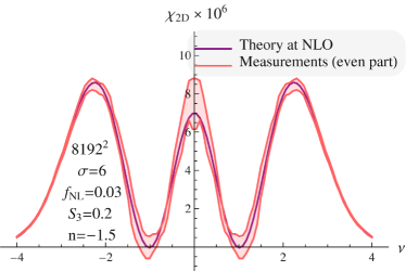
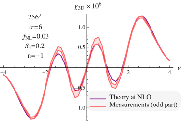
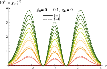
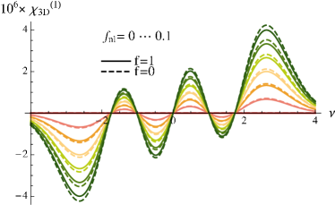
Figure 12: non-Gaussian part of the Euler characteristic of a mildly non-Gaussian anisotropic field in 2D (left panels) and 3D (right panels). The top panels compares the theoretical prediction to the measurements of realisations of the non-Gaussian fields with parameters as labeled, while the bottom panels illustrates the variation of the theory with the amplitude of $f_{\mathrm{{nl}}}$. The shaded area corresponds to the one sigma measurements error. The match to the theory is very good throughout. The effect of redshift distortion is clearly weaker in 3D, as expected.

Figure 13 shows how $g_{nl}$ acts in turn. For this purpose, the prediction at NNLO ($n=4$ in the Gram-Charlier expansion) is computed from equation (40).

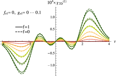
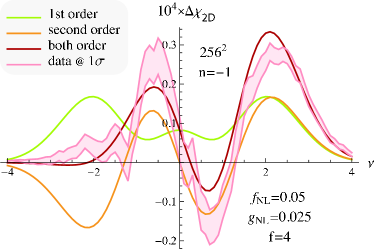
Figure 13: Left: variation with the amplitude of $g_{\mathrm{{nl}}}$ of the predicted Euler characteristic at NLO of a mildly 2D non-Gaussian anisotropic field. Right: match between a given realisation with $f_{\mathrm{{nl}}}$ and $g_{\mathrm{{nl}}}$ as labeled, and the corresponding model decomposed into first ($n=3$) and second order ($n=4$) corrections.

Finally, Figure 14 displays predictions and measurements for differential extrema counts in these kinds of $f_{nl}$ fields. As mentioned in the main text, at even orders in the GC expansion (in particular at Gaussian order), 2D saddle counts is even, peak and void counts are symetric by reflexion across the y-axis meaning $\partial_{\nu}n_{\rm peaks}(\nu)=\partial_{\nu}n_{\rm voids}(-\nu)$ and pancake and filament counts are also symetric by reflection across the y-axis. On the other hand, at odd orders in the GC expansion (in particular at first non-Gaussian order), the 2D saddle count is odd in $\nu$, peak and void counts are symmetric w.r.t. reflection relative to the origin, meaning $\partial_{\nu}n_{\rm peaks}(\nu)=-\partial_{\nu}n_{\rm voids}(-\nu)$ and pancake and filament counts are also symmetric by reflection relative to the origin. Figure 14 thus displays on left panels the even part of the data which should be dominated by the Gaussian term, namely $(\partial_{\ nu}n_{\rm sad}(\nu)+\partial_{\nu}n_{\rm sad}(-\nu))/2$ for 2D saddle points, $(\partial_{\nu}n_{\rm peaks}(\nu)+\partial_{\nu}n_{\rm voids}(-\nu))/2$ for peaks and $(\partial_{\nu}n_{\rm voids}(\nu)+\partial_{\nu}n_{\rm peaks}(-\nu))/2$ for voids (pancakes and filaments accordingly); and in the right panels, the even part of the measurement, namely $(\partial_{\nu}n_{\rm sad}(\nu)-\partial_{\nu}n_{\rm sad}(-\nu))/2$ for 2D saddle points, $(\partial_{\nu}n_{\rm peaks}(\nu)-\partial_{\nu}n_{\rm voids}(-\nu))/2$ for peaks and $(\partial_{\nu}n_{\rm voids}(\nu)-\partial_{\nu}n_{\rm peaks}(-\nu))/2$ for voids. Agreement between measurement and theory to NLO is very good. The small difference between both is due to NNLO correction and to a bias in the measurement of pancake counts which is yet to be fixed.

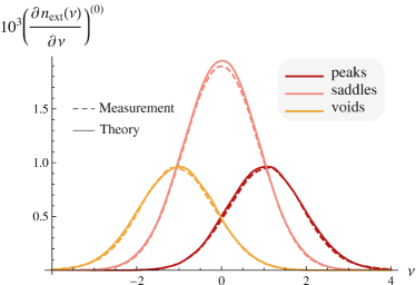
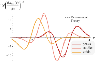
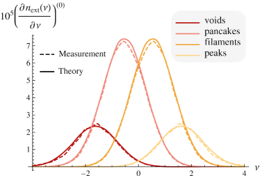
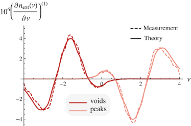
Figure 14: Top left panel: The distribution of 2D extrema (voids, saddles and peaks as labeled) as a function of threshold $\nu$ in redshift space for $f=1$ as predicted at Gaussian order (solid) and measured (“even part” of the data only, see main text for more details). Top right panel: the corresponding non-Gaussian correction ($f_{\mathrm{{nl}}}=0.05$) estimated from 20 realisations of the corresponding scale invariant (n=-1) field of dimension $4096^{2}$ smoothed over 4 pixels as predicted at first non-Gaussian order (solid) and measured (“odd part” of the data only). Bottom panels: Same as top panels for the distribution of 3D extrema (voids, wall saddles, tube saddle and peaks as labeled) for non-Gaussian scale-invariant ($n=-1$, $256^{3}$ smoothed over 4 pixels) anisotropic field ($f_{\mathrm{{nl}}}=0.07$, $f=1$).

B.2 $f_{\mathrm{{nl}}}$ model for the potential

In Astrophysics, $f_{nl}$ often refers to the potential from which the (density) field derives. Let us thus study in this section the effect of such $f_{nl}$ non-Gaussianities in the potential on the genus of the density field. If $\Phi$ is a Gaussian (possibly anisotropic) potential field with zero mean and variance $\left\langle\Phi^{2}\right\rangle=\sigma_{0}^{2}$, let us define the following non-Gaussian field

$$\Phi^{\mathrm{NG}}=\Phi+\frac{f_{\mathrm{{nl}}}}{\sigma_{0}}\left(\Phi^{2}-\sigma_{0}^{2}\right)\,.$$ (124)

Then the resulting non-Gaussian density field reads

$$\delta^{\mathrm{NG}}=\Delta\Phi^{\mathrm{NG}}=\Delta\Phi+2\frac{f_{\mathrm{{nl}}}}{\sigma_{0}}\left(\Phi\Delta\Phi+\nabla\Phi\cdot\nabla\Phi\right)\,.$$ (125)

For the purpose of this paper, let us define again the final density field as a Kaiser transform of this field (c.f. equation (11)) so that in Fourier space

$$\hat{\delta}_{k}=(1+f\mu^{2})\hat{\delta}^{\mathrm{NG}}_{k},\quad\mathrm{with}\quad\mu=k_{\parallel}/k.$$ (126)

Then any Minkowski functional or extrema count of this non-Gaussian field can be written in terms only of $f$, $f_{\mathrm{{nl}}}$ and $\sigma$’s (or $n$ for a scale invariant power spectrum). Figure 15 (top panels) shows the prediction for the 2D Euler characteristic for different values of $f_{\mathrm{{nl}}}$ between 0 and 1 and for $f=0$ (isotropic case) and $f=1$ (Kaiser). It also compares (bottom panels) the prediction with some measurements and shows a great agreement up to first order (the difference we observe must come from higher order corrections as the parity in Hermite polynomials is different).

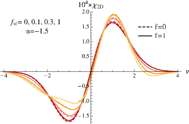
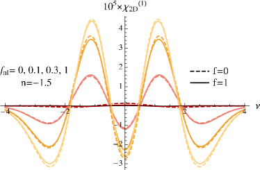
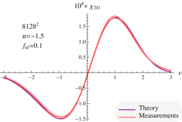
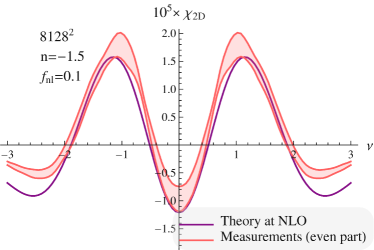
Figure 15: Top left: 2D Euler characteristic of the density field for $f_{\mathrm{{nl}}}$ between 0 (red) and 1 (yellow) in the potential field and $f=0$ (dashed line) or 1 (solid line). Top right: same as top left panel for the first non-Gaussian correction. Bottom left: 2D Euler characteristic of the density field for $f_{\mathrm{{nl}}}=0.1$ in the potential field. Measurements are displayed in pink with a shaded area representing the $1-\sigma$ dispersion and prediction in violet. Bottom right: same as left panel for the first non-Gaussian correction.

Appendix C 3D Euler characteristic at all orders in non-Gaussianity

To compute the 3D Euler characteristics, one needs to take into account the variable $\Upsilon$. Given that the Gram-Charlier polynomial expansion for the non-Gaussian PDF is obtained by using polynomials orthogonal with respect to the kernel provided by the JPDF in the Gaussian limit, the coupling between $\Upsilon$ and $Q^{2},J_{2\perp}$ variables in the Gaussian limit introduces a set of polynomials $F_{lrs}$ such that

$$\frac{1}{\pi}\int\mathrm{d}J_{2\perp}\,\mathrm{d}Q^{2}\frac{d\Upsilon}{\sqrt{Q^{4}J_{2\perp}-\Upsilon^{2}}}e^{-J_{2\perp}-Q^{2}}F_{lrs}\!\left(J_{2\perp},Q^{2},\Upsilon\right)F_{l^{\prime}r^{\prime}s^{\prime}}\!\left(J_{2\perp},Q^{2},\Upsilon\right)=\delta_{ll^{\prime}}\delta_{rr^{\prime}}\delta_{ss^{\prime}}.$$ (127)

Here $l$ is the power of $J_{2\perp}$, $r$ the power of $Q^{2}$ and $s$ the power of $\Upsilon$. In particular, $F_{lr0}\!\left(J_{2\perp},Q^{2},\Upsilon\right)=L_{l}\!\left(J_{2\perp}\right)L_{r}\!\left(Q^{2}\right)$ and $F_{001}\!\left(J_{2\perp},Q^{2},\Upsilon\right)=H_{1}\!\left(\Upsilon\right)$.

The full expansion of non-Gaussian JPDF $P=P(x,q^{2}_{\perp},x_{3},\zeta,J_{2\perp},\xi,Q^{2},\Upsilon)$ is a series of products of $F_{lrs}$ and familiar Hermite and Laguerre polynomials for the rest of the variables, namely

$$P=G\!\left[1+\!\sum_{n=3}^{\infty}\sum_{\sigma_{n}}\!\frac{(-1)^{j+l+r}g_{lrs}}{i!\;j!\;k!\;l!\;m!\;r!\;p!\;s!}\!\left\langle x^{i}{q^{2j}_{\perp}}{\zeta}^{k}x_{3}^{m}\xi^{p}J^{l}_{2\perp}Q^{2r}\Upsilon^{s}\right\rangle_{\!\mathrm{GC}}\!\!\!\!\!\!H_{i}\!\left(x\right)\!L_{j}\!\left(q_{\perp}^{2}\right)\!H_{k}\!\left(\zeta\right)\!H_{m}\!\left(x_{3}\right)\!H_{p}\!\left(\xi\right)\!F_{lrs}\!\left(J_{2\perp},Q^{2},\Upsilon\right)\right],$$ (128)

where $\sigma_{n}=\{(i,j,k,l,m,p,r,s)\in\mathbb{N}^{7}|i+2j+k+2l+m+2r+p+3s=n\}$ and $G$ is given by equation (18). The terms of the expansion 128 are sorted in the order of power in field variables $n$. We immediately see that at $n=3$ order, the only contribution from $\Upsilon$ comes from the term corresponding to $i=j=l=m=p=r=0,s=1$.

The Gram-Charlier coefficients are defined by

$$\left\langle x^{i}{q^{2j}_{\perp}}{\zeta}^{k}x_{3}^{m}\xi^{p}J^{l}_{2\perp}Q^{2r}\Upsilon^{s}\right\rangle_{\!\mathrm{GC}}=\frac{(-1)^{j+l+r}}{g_{lrs}}j!\,l!\,r!\,s!\left\langle H_{i}\!\left(x\right)\!L_{j}\!\left(q_{\perp}^{2}\right)\!H_{k}\!\left(\zeta\right)\!H_{m}\!\left(x_{3}\right)\!H_{p}\!\left(\xi\right)\!F_{lrs}\!\left(J_{2\perp},Q^{2},\Upsilon\right)\right\rangle\,,$$ (129)

where $g_{lrs}$ is such that the highest power term in $F_{lrs}\!\left(J_{2\perp},Q^{2},\Upsilon\right)$ is $(-1)^{l+r}g_{lrs}J_{2\perp}^{l}Q^{2r}\Upsilon^{s}/(l!r!s!)$. Amongst them, we have in particular $g_{lr0}=1$ and $g_{001}=1$. From equation (31), it is clear that the 3D Euler characteristic is the sum of a term where Upsilon can be marginalized over (so that the formalism introduced in Section 3 can be used) and a term which integrates $\Upsilon$ under the condition of zero gradient. This latter part is simply computed because $\Upsilon=F_{001}(J_{2\perp},Q^{2},\Upsilon)$ is orthogonal to all other $F_{lrs}$ polynomials in the Gram-Charlier expansion of the JPDF. After some algebra, it is found that the full 3D Euler characteristic can be eventually written

$$\chi_{\mathrm{3D}}(\nu)=\frac{e^{-\nu^{2}/2}}{8\pi^{2}}\frac{\sigma_{1\parallel}\sigma_{1\perp}^{2}}{\sigma^{3}}H_{2}(\nu)+\sum_{n=3}^{\infty}\chi_{\mathrm{3D}}^{(n)}\,,$$ (130)

with $\chi_{\mathrm{3D}}^{(n)}$ given by

$$\chi_{\mathrm{3D}}^{(n)}(\nu)=\frac{e^{-\nu^{2}/2}}{8\pi^{2}}\frac{\sigma_{2\perp}^{2}\sigma_{2\parallel}}{\sigma_{1\perp}^{2}\sigma_{1\parallel}}\Bigg{[}\sum_{\sigma_{n}}\frac{(-1)^{j+m}}{2^{m}i!\;j!\;m!}H_{i+2}(\nu)\gamma_{\parallel}\gamma_{\perp}^{2}\left\langle x^{i}q^{2j}_{\perp}x_{3}^{2m}\right\rangle_{\mathrm{GC}}-\sum_{\sigma_{n-1}}\frac{(-1)^{j+m}}{2^{m}i!\;j!\;m!}H_{i+1}(\nu)\left\langle x^{i}q^{2j}_{\perp}x_{3}^{2m}\left(\gamma_{\perp}^{2}x_{33}+2\gamma_{\perp}\gamma_{\parallel}J_{1\perp}\right)\right\rangle_{\mathrm{GC}}$$ (131)

$$+\!\!\sum_{\sigma_{n-2}}\!\!\frac{(-1)^{j+m}}{2^{m}i!\;j!\;m!}H_{i}(\nu)\!\left\langle x^{i}q^{2j}_{\perp}x_{3}^{2m}\left(2\gamma_{\perp}(J_{1\perp}x_{33}-\gamma_{2}Q^{2})+\gamma_{\parallel}(J_{1\perp}^{2}-{J_{2\perp}})\right)\right\rangle_{\!\mathrm{G}C}-\sum_{\sigma_{n-3}}\!\!\frac{(-1)^{j+m}}{2^{m}i!\;j!\;m!}H_{i-1}\!\left(\nu\right)\left\langle x^{i}q^{2j}_{\perp}x_{3}^{2m}\left(4I_{3}\right)\right\rangle_{\mathrm{\!\!GC}}\Bigg{]}\,,$$ (132)

where $I_{3}=\frac{1}{4}x_{33}(J^{2}_{1\perp}-J_{2\perp})-\frac{1}{2}\gamma_{2}\left(Q^{2}J_{1\perp}-\Upsilon\right)$. In equation (132), the Gram-Charlier coefficients are written in a concise form but must be interpreted returning from the $(x,x_{33},J_{1\perp})$ to the $(x,\zeta,\xi)$ variables and using equation (20). In the isotropic limit the result is reduced to the following compact form

$$\chi_{\mathrm{3D}}^{(n)}(\nu)=\frac{e^{-\nu^{2}/2}}{8\pi^{2}}\frac{\sigma_{1}^{3}}{\sigma^{3}}\Bigg{[}\frac{2}{3\sqrt{3}}\sum_{\sigma_{n}}\frac{(-1)^{j+m}}{2^{m}i!\;j!\;m!}H_{i+2}(\nu)\left\langle x^{i}q^{2j}_{\perp}x_{3}^{2m}\right\rangle_{\mathrm{GC}}-\frac{2}{\sqrt{3}}\gamma^{-1}\sum_{\sigma_{n-1}}\frac{(-1)^{j+m}}{2^{m}i!\;j!\;m!}H_{i+1}(\nu)\left\langle x^{i}q^{2j}_{\perp}x_{3}^{2m}I_{1}\right\rangle_{\mathrm{GC}}\\ +2\sqrt{3}\gamma^{-2}\!\!\sum_{\sigma_{n-2}}\!\!\frac{(-1)^{j+m}}{2^{m}i!\;j!\;m!}H_{i}(\nu)\!\left\langle x^{i}q^{2j}_{\perp}x_{3}^{2m}I_{2}\right\rangle_{\!\mathrm{G}C}-\frac{16}{5}\sqrt{\frac{3}{5}}\gamma^{-3}\sum_{\sigma_{n-3}}\!\!\frac{(-1)^{j+m}}{2^{m}i!\;j!\;m!}H_{i-1}\!\left(\nu\right)\left\langle x^{i}q^{2j}_{\perp}x_{3}^{2m}I_{3}\right\rangle_{\mathrm{\!\!GC}}\Bigg{]}\,,$$ (133)

where $I_{1}$, $I_{2}$ and $I_{3}$ are the 3 invariants of the Hessian matrix $x_{ij}$, namely $I_{1}=J_{1}=\lambda_{1}+\lambda_{2}+\lambda_{3}=\mathrm{Tr}\,x_{ij}$, $I_{2}=\lambda_{1}\lambda_{2}+\lambda_{2}\lambda_{3}+\lambda_{3}\lambda_{1}$ and $I_{3}=\lambda_{1}\lambda_{2}\lambda_{3}=\det x_{ij}$. Note that equations (132) and (133) contain some $H_{-1}(\nu)=\sqrt{\pi/2}\textrm{ Erfc}(\nu/\sqrt{2})$ which are shown to contribute as a boundary term and can thus be factorized out of the terms $\chi_{\mathrm{3D}}^{(n)}$ as mentioned in equation (33). Moreover, the well known topological relation between the Euler characteristics and the genus allows us to compare the above quantity with the curvature integrated along isocontours (as used in Matsubara (1996)). In an anisotropic space, this surface integral is found to be

$$\chi_{\mathrm{3D}}^{\mathrm{s}}(\nu)=\frac{e^{-\nu^{2}/2}}{8\pi^{2}}\frac{\sigma_{1||}\sigma_{1\perp}^{2}}{\sigma^{3}}\Bigg{[}H_{2}(\nu)+\frac{1}{\gamma_{\perp}^{2}}\sum_{n=3}^{\infty}\sum_{\sigma_{n-2}}\!\!\!\frac{(-1)^{j+m}}{i!\;j!m!(2m\!-\!1)2^{m}}H_{i}(\nu)\left(\left\langle x^{i}q^{2j}_{\perp}{J_{2\perp}}\,x_{3}^{2m}\right\rangle_{\!\mathrm{GC}}\!\!\!\!-(1-\gamma_{\perp}^{2})\left\langle x^{i}q^{2j}_{\perp}\zeta^{2}x_{3}^{2m}\right\rangle_{\!\mathrm{GC}}\right)\\ +2\frac{\sqrt{1\!-\!\gamma_{\perp}^{2}}}{\gamma_{\perp}}\sum_{n=3}^{\infty}\sum_{\sigma_{n-1}}\!\!\!\frac{(-1)^{j+m}}{i!\;j!m!(2m\!-\!1)2^{m}}\!\left\langle x^{i}q^{2j}_{\perp}\zeta\,x_{3}^{2m}\right\rangle_{\!\mathrm{GC}}\!\!\!\!\!\!\!\!H_{i}(\nu)H_{1}(\nu)\!-\!\sum_{n=3}^{\infty}\sum_{\sigma_{n}}\!\frac{(-1)^{j+m}}{i!\;j!m!(2m\!-\!1)2^{m}}\!\left\langle x^{i}q^{2j}_{\perp}x_{3}^{2m}\right\rangle_{\!\mathrm{GC}}\!\!\!\!\!\!\!\!H_{i}(\nu)H_{2}(\nu)\!\Bigg{]}\,,$$ (134)

where we use the convention $(-2)!/(-1)!=-1/2$. Equations (130) and (134) were checked to be equivalent up to at least $n=4$ using some detailed relations between the cumulants (which once again can be established via integrations by parts) assuming that everything vanishes at infinity (in particular $\chi_{\mathrm{3D}}(-\infty)=0$). Note that in this expression $\xi$, $Q^{2}$ and $\Upsilon$ do not appear anymore.

References

- Adler (1981) Adler R. J., 1981, The Geometry of Random Fields. Chichester: Wiley
- Amendola (1996) Amendola L., 1996, MNRAS, 283, 983
- Bardeen et al. (1986) Bardeen J. M., Bond J. R., Kaiser N., Szalay A. S., 1986, ApJ, 304, 15
- Bernardeau & Brax (2011) Bernardeau F., Brax P., 2011, JCAP, 6, 19
- Bernardeau et al. (2002) Bernardeau F., Colombi S., Gaztañaga E., Scoccimarro R., 2002, Physics Reports, 367, 1
- Bernardeau & Kofman (1995) Bernardeau F., Kofman L., 1995, ApJ, 443, 479
- Blinnikov & Moessner (1998) Blinnikov S., Moessner R., 1998, Astronomy and Astrophysics Supplement, 130, 193
- Bond & Efstathiou (1987) Bond J. R., Efstathiou G., 1987, MNRAS, 226, 655
- Chambers (1967) Chambers J. M., 1967, Biometrika, 54, 367
- Clifton et al. (2012) Clifton T., Ferreira P. G., Padilla A., Skordis C., 2012, physics repport, 513, 1
- Coles (1988) Coles P., 1988, MNRAS, 234, 509
- Colombi et al. (2000) Colombi S., Pogosyan D., Souradeep T., 2000, Physical Review Letters, 85, 5515
- Cramér (1946) Cramér H., 1946, Mathematical Methods of Statistics. Princeton Univ. Press
- Desjacques & Sheth (2010) Desjacques V., Sheth R. K., 2010, Phys. Rev. D, 81, 023526
- Doroshkevich (1970) Doroshkevich A. G., 1970, Astrofizika, 6, 581
- Gay et al. (2012) Gay C., Pichon C., Pogosyan D., 2012, Phys. Rev. D, 85, 023011
- Gaztañaga et al. (2009) Gaztañaga E., Cabré A., Castander F., Crocce M., Fosalba P., 2009, MNRAS, 399, 801
- Gott (1988) Gott III J. R., 1988, Publication of the Astronomical Society of the Pacific, 100, 1307
- Gott et al. (1989) Gott III J. R., Miller J., Thuan T. X., Schneider S. E., Weinberg D. H., Gammie C., Polk K., Vogeley M., Jeffrey S., Bhavsar S. P., Melott A. L., Giovanelli R., Hayes M. P., Tully R. B., Hamilton A. J. S., 1989, ApJ, 340, 625
- Gott et al. (1990) Gott III J. R., Park C., Juszkiewicz R., Bies W. E., Bennett D. P., Bouchet F. R., Stebbins A., 1990, ApJ, 352, 1
- Gott et al. (1987) Gott III J. R., Weinberg D. H., Melott A. L., 1987, ApJ, 319, 1
- Gott et al. (2007) Gott J. R. I., Colley W. N., Park C.-G., Park C., Mugnolo C., 2007, MNRAS, 377, 1668
- Hadwiger (1957) Hadwiger H., 1957, Vorlesungen über Inhalt, Oberfläche und Isoperimetrie. Springer
- Hamilton et al. (1986) Hamilton A. J. S., Gott III J. R., Weinberg D., 1986, ApJ, 309, 1
- Heyvaerts et al. (2013) Heyvaerts J., Pichon C., Prunet S., Thiébaut J., 2013, MNRAS, 430, 3320
- Hikage et al. (2003) Hikage C., Schmalzing J., Buchert T., Suto Y., Kayo I., Taruya A., Vogeley M. S., Hoyle F., Gott III J. R., Brinkmann J., 2003, PASJ, 55, 911
- Hikage et al. (2002) Hikage C., Suto Y., Kayo I., Taruya A., Matsubara T., Vogeley M. S., Hoyle F., Gott III J. R., Brinkmann J., 2002, PASJ, 54, 707
- Hivon et al. (1995) Hivon E., Bouchet F. R., Colombi S., Juszkiewicz R., 1995, A&A, 298, 643
- Huchra & Geller (1982) Huchra J. P., Geller M. J., 1982, ApJ, 257, 423
- Jackson (1972) Jackson J. C., 1972, MNRAS, 156, 1P
- Jost (2008) Jost J., 2008, Riemannian Geometry and Geometric Analysis, Fifth Edition. Berlin ; New York : Springer, c2008.
- Juszkiewicz et al. (1995) Juszkiewicz R., Weinberg D. H., Amsterdamski P., Chodorowski M., Bouchet F., 1995, ApJ, 442, 39
- Kaiser (1984) Kaiser N., 1984, ApJ Let., 284, L9
- Kaiser (1987) Kaiser N., 1987, MNRAS, 227, 1
- Kendall & Stuart (1958) Kendall M. G., Stuart A., 1958, The Advanced Theory of Statistics. Vol. 1, London: Griffin
- Laureijs et al. (2011) Laureijs R., Amiaux J., Arduini S., Auguères J. ., Brinchmann J., Cole R., Cropper M., Dabin C., Duvet L., Ealet A., et al. 2011, ArXiv e-prints
- Lazarian & Pogosyan (2000) Lazarian A., Pogosyan D., 2000, ApJ, 537, 720
- Matsubara (1994) Matsubara T., 1994, ApJ Let., 434, L43
- Matsubara (1996) Matsubara T., 1996, ApJ, 457, 13
- Matsubara (2003) Matsubara T., 2003, ApJ, 584, 1
- Matsubara (2010) Matsubara T., 2010, Phys. Rev. D, 81, 083505
- Matsubara & Suto (1995) Matsubara T., Suto Y., 1995, Arxiv preprint astro-ph/9509129, p. 20
- Mecke et al. (1994) Mecke K. R., Buchert T., Wagner H., 1994, A&A, 288, 697
- Melott et al. (1989) Melott A. L., Cohen A. P., Hamilton A. J. S., Gott III J. R., Weinberg D. H., 1989, ApJ, 345, 618
- Melott et al. (1988) Melott A. L., Weinberg D. H., Gott III J. R., 1988, ApJ, 328, 50
- Nishimichi et al. (2010) Nishimichi T., Taruya A., Koyama K., Sabiu C., 2010, JCAP, 7, 2
- Novikov et al. (2003) Novikov D., Colombi S., Doré O., 2003, Monthly Notices of the Royal Astronomical Society, 366, 15
- Park et al. (2005) Park C., Choi Y.-Y., Vogeley M. S., Gott J. R. I., Kim J., Hikage C., Matsubara T., Park M.-G., Suto Y., Weinberg D. H., 2005, ApJ, 633, 11
- Peebles (1980) Peebles P. J. E., 1980, The large-scale structure of the universe. Princeton University Press
- Percival et al. (2007) Percival W. J., Cole S., Eisenstein D. J., Nichol R. C., Peacock J. A., Pope A. C., Szalay A. S., 2007, MNRAS, 381, 1053
- Planck Collaboration et al. (2013) Planck Collaboration Ade P. A. R., Aghanim N., Armitage-Caplan C., Arnaud M., Ashdown M., Atrio-Barandela F., Aumont J., Baccigalupi C., Banday A. J., et al. 2013, ArXiv e-prints
- Pogosyan et al. (2009) Pogosyan D., Gay C., Pichon C., 2009, Phys. Rev. D, 80, 081301
- Pogosyan et al. (2011) Pogosyan D., Pichon C., Gay C., 2011, Phys. Rev. D, 84, 083510
- Pogosyan et al. (2009) Pogosyan D., Pichon C., Gay C., Prunet S., Cardoso J. F., Sousbie T., Colombi S., 2009, MNRAS, pp 673–+
- Rice (1944) Rice S. O., 1944, Bell Systems Tech. J., Volume 23, p. 282-332, 23, 282
- Rice (1945) Rice S. O., 1945, Bell Systems Tech. J., Volume 24, p. 46-156, 24, 41
- Ryden (1988) Ryden B. S., 1988, ApJ Let., 333, L41
- Ryden et al. (1989) Ryden B. S., Melott A. L., Craig D. A., Gott III J. R., Weinberg D. H., Scherrer R. J., Bhavsar S. P., Miller J. M., 1989, ApJ, 340, 647
- Sargent & Turner (1977) Sargent W. L. W., Turner E. L., 1977, ApJ Let., 212, L3
- Scaramella & Vittorio (1991) Scaramella R., Vittorio N., 1991, ApJ, 375, 439
- Scoccimarro (2004) Scoccimarro R., 2004, Phys. Rev. D, 70, 083007
- Scoccimarro et al. (1998) Scoccimarro R., Colombi S., Fry J. N., Frieman J. A., Hivon E., Melott A., 1998, ApJ, 496, 586
- Scoccimarro et al. (1999) Scoccimarro R., Couchman H. M. P., Frieman J. A., 1999, ApJ, 517, 531
- Seto (2000) Seto N., 2000, ApJ, 538, 11
- Spergel et al. (2003) Spergel D. N., Verde L., Peiris H. V., Komatsu E., Nolta M. R., Bennett C. L., Halpern M., Hinshaw G., Jarosik N., Kogut A., Limon M., Meyer S. S., Page L., Tucker G. S., Weiland J. L., Wollack E., Wright E. L., 2003, ApJ Sup., 148, 175
- Taruya et al. (2010) Taruya A., Nishimichi T., Saito S., 2010, Phys. Rev. D, 82, 063522
- Teyssier (2002) Teyssier R., 2002, A&A, 385, 337
- Teyssier et al. (2009) Teyssier R., Pires S., Prunet S., Aubert D., Pichon C., Amara A., Benabed K., Colombi S., Refregier A., Starck J.-L., 2009, A&A, 497, 335
- Verde et al. (1998) Verde L., Heavens A. F., Matarrese S., Moscardini L., 1998, MNRAS, 300, 747
- Wang et al. (2012) Wang X., Chen X., Park C., 2012, ApJ, 747, 48
- Weinberg et al. (1987) Weinberg D. H., Gott III J. R., Melott A. L., 1987, ApJ, 321, 2
- Zunckel et al. (2011) Zunckel C., Gott J. R., Lunnan R., 2011, MNRAS, 412, 1401